Gravitational collapse and formation of universal horizons

Abstract

In this paper, we first generalize the definition of stationary universal horizons to dynamical ones, and then show that (dynamical) universal horizons can be formed from realistic gravitational collapse. This is done by constructing analytical models of a collapsing spherically symmetric star with finite thickness in Einstein-aether theory.

I Introduction

The invariance under the Lorentz symmetry group is a cornerstone of modern physics, and is strongly supported by observations. In fact, all the experiments carried out so far are consistent with it Liberati13 , and no evidence to show that such a symmetry must be broken at certain energy scales, although it is arguable that such constraints in the gravitational sector are much weaker than those in the matter sector LZbreaking .

Nevertheless, there are various reasons to construct gravitational theories with broken Lorentz invariance (LI) LACW . In particular, our understanding of space-times at Plank scale is still highly limited, and the renomalizability and unitarity of gravity often lead to the violation of LI QGs . One concrete example is the Hořava theory of quantum gravity Horava , in which the LI is broken via the anisotropic scaling between time and space in the ultraviolet (UV),

$$t\rightarrow b^{-z}t,\;\;\;x^{i}\rightarrow b^{-1}x^{i},\;(i=1,2,3),$$ (1.1)

where $z$ denotes the dynamical critical exponent. This is a reminiscent of Lifshitz scalars in condensed matter physics Lifshitz , hence the theory is often referred to as the Hořava-Lifshitz (HL) quantum gravity at a Lifshitz fixed point. The anisotropic scaling (1.1) provides a crucial mechanism: The gravitational action can be constructed in such a way that only higher-dimensional spatial (but not time) derivative operators are included, so that the UV behavior of the theory is dramatically improved. In particular, for $z\geq 3$ it becomes power-counting renormalizable Horava ; Visser . The exclusion of high-dimensional time derivative operators, on the other hand, prevents the ghost instability, whereby the unitarity of the theory is assured Stelle . In the infrared (IR) the lower dimensional operators take over, and a healthy low-energy limit is presumably resulted . It is remarkable to note that, despite of the stringent observational constraints of the violation of the LI Liberati13 , the nonrelativistic general covariant HL gravity constructed in ZWWS is consistent with all the solar system tests Will ; LMWZ and cosmology cosmo ; ZHW . In addition, it has been recently embedded in string theory via the nonrelativistic AdS/CFT correspondence JK . Another version of the HL gravity, the health extension BPS , is also self-consistent and passes all the solar system, astrophysical and cosmological tests .

Another example that violates LI is the Einstein-aether theory, in which the breaking is realized by a timelike vector field, while the gravitational action is still generally covariant EA . This theory is consistent with all the solar system tests EA and binary pulsar observations Yagi .

However, once the LI is broken, speeds of particles can be greater than that of light. In particular, the dispersion relation generically becomes nonlinear ZHW ,

$$E^{2}=c_{p}^{2}p^{2}\left(1+\alpha_{1}\left(\frac{p}{M_{*}}\right)^{2}+\alpha_{2}\left(\frac{p}{M_{*}}\right)^{4}\right),$$ (1.2)

where $E$ and $p$ are the energy and momentum of the particle considered, and $c_{p},\;\alpha_{i}$ are coefficients, depending on the species of the particle, while $M_{*}$ denotes the suppression energy scale of the higher-dimensional operators. Then, one can see that both phase and group velocities of the particles are unbounded with the increase of energy. This suggests that black holes may not exist at all in theories with broken LI, and makes such theories questionable, as observations strongly indicate that black holes exist in our universe NM .

Lately, a potential breakthrough was the discovery that there still exist absolute causal boundaries, the so-called universal horizons, in the theories with broken LI BS11 . Particles even with infinitely large velocities would just move around on these boundaries and cannot escape to infinity UHs . The universal horizon radiates like a blackbody at a fixed temperature, and obeys the first law of black hole mechanics BBM .

Recently, we studied the existence of universal horizons in the three well-known black hole solutions, the Schwarzschild, Schwarzschild anti-de Sitter, and Reissner-Nordström, and found that in all of them universal horizons always exist inside their Killing horizons LGSW . In particular, the peeling-off behavior of the globally timelike khronon field $u_{\mu}$ was found only at the universal horizons, whereby the surface gravity $\kappa_{\text{peeling}}$ is calculated and found equal to CLMV ,

$$\kappa_{\text{UH}}\equiv\frac{1}{2}u^{\alpha}D_{\alpha}\left(u_{\lambda}\zeta^{\lambda}\right),$$ (1.3)

where $\zeta^{\mu}$ and $D_{\mu}$ denote, respectively, the time translation Killing field and covariant derivative with respect to the given space-time metric $g_{\mu\nu}\;(\mu,\nu=0,1,2,3)$. For the Schwarzschild solution, the universal horizon and surface gravity are given, respectively, by LGSW ,

$$R_{UH}^{\text{Sch.}}=\frac{3r_{s}}{4},\;\;\;\kappa_{\text{peeling}}^{\text{Sch.}}=\left(\frac{2}{3}\right)^{3/2}\frac{1}{r_{s}},$$ (1.4)

where $r_{s}$ denotes the Schwarzschild radius.

In this paper, we shall study the formation of the universal horizons from realistic gravitational collapse of a spherically symmetric star . To be more concrete, we shall consider such a collapsing object in the Einstein-aether theory EA . To make the problem tractable, we further assume that the effects of the aether are negligible, so the space-time outside of the star is still described by the Schwarzschild solution, while inside the star we assume that the distribution of the matter is homogeneous and isotropic, so the internal space-time is that of the Friedmann-Robertson-Walker (FRW). Although the model is very ideal, it is sufficient to serve our current purposes, that is, to show explicitly that universal horizons can be formed from realistic gravitational collapse.

Specifically, the paper is organized as follows: In Sec. II, we shall present a brief review on the definition of the stationary universal horizons, and then generalize it to dynamical spacetimes. This is realized by replacing Killing horizons by apparent horizons Hayd ; Wang , and in the stationary limit, the latter reduces to the former. In Sec. III, we study a collapsing spherically symmetric star with a finite thickness in the framework of the Einstein-aether theory. When the effects of the aether are negligible, the vacuum space-time outside the star is uniquely described by the Schwarzschild solution and the junction condition across the surface of the star reduces to those of Israel IC66 . Once this is done, we find that the khronon equation can be solved analytically when the speed of the khronon is infinitely large, for which the sound horizon of the khronon coincides with the universal horizon. It is remarkable that this is also the case for the Schwarzschild solution LGSW , for which the universal horizon and surface gravity are given by Eq.(1.4). The paper is ended in Sec. IV, in which our main conclusions are presented.

II Dynamical universal horizons and black holes

A necessary condition for the existence of a universal horizon of a given space-time is the existence of a globally time-like foliation BS11 ; LACW ; LGSW . This foliation is usually characterized by a scalar field $\phi$, dubbed khronon BS11 , and the normal vector $u_{\mu}$ of the foliation is always time-like,

$$u^{\lambda}u_{\lambda}=-1,$$ (2.1)

where

$$u_{\mu}=\frac{\phi_{,\mu}}{\sqrt{X}},\;\;\;\phi_{,\mu}\equiv\frac{\partial\phi}{\partial x^{\mu}},\;\;\;X\equiv-g^{\alpha\beta}\partial_{\alpha}\phi\partial_{\beta}\phi.$$ (2.2)

In this paper, we choose the signature of the metric as ($-1,1,1,1$). It is important to note that such a defined khronon field is unique only up to the following gauge transformation,

$$\tilde{\phi}={\cal{F}}(\phi),$$ (2.3)

where ${\cal{F}}(\phi)$ is a monotonically increasing (or decreasing) and otherwise arbitrary function of $\phi$. Clearly, under the above gauge transformations, we have $\tilde{u}_{\mu}=u_{\mu}$.

The khronon field $\phi$ is described by the action EA ,

$$S_{\phi} = \int d^{4}x\sqrt{|g|}\Big{[}V_{0}\left(D_{\mu}u_{\nu}\right)^{2}+V_{0}\left(D_{\mu}u^{\mu}\right)^{2}$$ (2.4)

$$~{}~{}+c_{3}\left(D^{\mu}u^{\nu}\right)\left(D_{\nu}u_{\mu}\right)-c_{4}a^{\mu}a_{\mu}\Big{]},$$

where $c_{i}$’s are arbitrary constants, and $a_{\mu}\equiv u^{\alpha}D_{\alpha}u_{\mu}$. The operator $D_{\mu}$ denotes the covariant derivative with respect to the background metric $g_{\mu\nu}$, as mentioned above. Note that the above action is the most general one in the sense that the resulting differential equations in terms of $u_{\mu}$ are second-order EA . However, when $u_{\mu}$ is written in the form of Eq.(2.2), the relation

$$u_{[\nu}D_{\alpha}u_{\beta]}=0,$$ (2.5)

is identically satisfied. Then, it can be shown that only three of the four coupling constants $c_{i}$ are independent. In fact, from Eq.(2.5) we find EA ,

$$\Delta{\cal{L}}_{\phi}\equiv a^{\mu}a_{\mu}+\big{(}D_{\alpha}u_{\beta}\big{)}\big{(}D^{\alpha}u^{\beta}\big{)}-\big{(}D_{\alpha}u_{\beta}\big{)}\big{(}D^{\beta}u^{\alpha}\big{)}=0.$$ (2.6)

Then, one can always add the term,

$$\Delta{S}_{\phi}=c_{0}\int{\sqrt{|g|}\;d^{4}x\Delta{\cal{L}}_{\phi}},$$ (2.7)

into $S_{\phi}$, where $c_{0}$ is an arbitrary constant. This is effectively to shift the coupling constants $c_{i}$ to ${c}_{i}^{\prime}$, where

$${c}_{1}^{\prime}=c_{1}+c_{0},\;{c}_{2}^{\prime}=c_{2},\;{c}_{3}^{\prime}=c_{3}-c_{0},\;{c}_{4}^{\prime}=c_{4}-c_{0}.$$ (2.8)

Thus, by properly choosing $c_{0}$, one can always set one of $c_{i}\;(i=1,3,4)$ to zero. However, in the following we shall leave this possibility open.

The variation of $S_{\phi}$ with respect to $\phi$ yields the khronon equation,

$$D_{\mu}{\cal{A}}^{\mu}=0,$$ (2.9)

where Wang13 ,

$${\cal{A}}^{\mu} \equiv \frac{\left(\delta^{\mu}_{\nu}+u^{\mu}u_{\nu}\right)}{\sqrt{X}}\AE^{\nu},$$

$$\AE^{\nu} \equiv D_{\gamma}J^{\gamma\nu}+c_{4}a_{\gamma}D^{\nu}u^{\gamma},$$

$$J^{\alpha}_{\;\;\;\mu} \equiv \big{(}V_{0}g^{\alpha\beta}g_{\mu\nu}+V_{0}\delta^{\alpha}_{\mu}\delta^{\beta}_{\nu}+c_{3}\delta^{\alpha}_{\nu}\delta^{\beta}_{\mu}$$ (2.10)

$$~{}~{}~{}-c_{4}u^{\alpha}u^{\beta}g_{\mu\nu}\big{)}D_{\beta}u^{\nu}.$$

II.1 Universal Horizons in Stationary and Asymptotically flat Spacetimes

In stationary and asymptotically flat spacetimes, there always exists a time translation Killing vector, $\zeta^{\mu}$, which is timelike asymptotically,

$$\zeta^{\lambda}\zeta_{\lambda}<0,$$ (2.11)

for $r\rightarrow\infty$. A Killing horizon is defined as the existence of a hypersurface on which the time translation Killing vector $\zeta^{\mu}$ becomes null,

$$\zeta^{\lambda}\zeta_{\lambda}=0.$$ (2.12)

On the other hand, a universal horizon is defined as the existence of a hypersurface on which $\zeta^{\mu}$ becomes orthogonal to $u_{\mu}$,

$$u_{\lambda}\zeta^{\lambda}=0.$$ (2.13)

Since $u_{\mu}$ is timelike globally, Eq.(2.13) is possible only when $\zeta_{\mu}$ becomes spacelike. This can happen only inside the apparent horizons, because only in that region $\zeta_{\mu}$ becomes spacelike.

II.2 Universal Horizons in Non-Stationary Spacetimes

To study the formation of universal horizons from gravitational collapse, we need first to generalize the above definition of the universal horizons to non-stationary spacetimes. For the sake of simplicity, in the rest of this paper we shall restrict ourselves only to spherical space-times, and its generalization to other spacetimes is straightforward.

The metric for a specially symmetric space-time can be cost in the form,

$$ds^{2}=g_{ij}dx^{i}dx^{j}+{R}^{2}\left(x^{i}\right)d\Omega^{2},\;(i,j=0,1),$$ (2.14)

in the spherical coordinates, $x^{\mu}=\left(x^{0},x^{1},\theta,\varpi\right),\;(\mu=0,1,2,3)$, where $d\Omega^{2}=d\theta^{2}+\sin^{2}\theta d\varpi^{2}$.

The normal vector $n_{\mu}$ to the hypersurface ${R}=C_{0}$ is given by,

$$n_{\mu}\equiv\frac{\partial({R}-C_{0})}{\partial x^{\mu}}=\delta^{0}_{\mu}{R}_{0}+\delta^{1}_{\mu}{R}_{1},$$ (2.15)

where $C_{0}$ is a constant and ${R}_{i}\equiv\partial{R}/\partial x^{i}$. Setting

$$\zeta^{\mu}=\delta^{0}_{\mu}{R}_{1}-\delta^{1}_{\mu}{R}_{0},$$ (2.16)

we can see that $\zeta^{\mu}$ is always orthogonal to $n_{\mu}$,

$$\zeta^{\lambda}n_{\lambda}=0.$$ (2.17)

For spacetimes that are asymptotically flat there always exists a region, say, ${R}>{R}_{\infty}$, in which $n_{\mu}$ and $\zeta^{\mu}$ are, respectively, space- and time-like, that is, $\left.n_{\mu}n^{\mu}\right|_{{R}>{R}_{\infty}}>0$ and $\left.\zeta^{\mu}\zeta_{\mu}\right|_{{R}>{R}_{\infty}}<0$. An apparent horizon may form at ${R}_{AH}$, at which $n_{\mu}$ becomes null,

$$\left.n_{\lambda}n^{\lambda}\right|_{{R}={R}_{AH}}=0,$$ (2.18)

where ${R}_{AH}<{R}_{\infty}$. Then, in the internal region ${R}<{R}_{AH}$, $n_{\mu}$ becomes timelike. Therefore, we have

$$n_{\lambda}n^{\lambda}=\cases{>0,&${R}>{R}_{AH}$,\cr=0,&${R}={R}_{AH}$,\cr<0,&${R}<{R}_{AH}$.\cr}$$ (2.19)

Since Eq.(2.17) always holds, we must have

$$\zeta_{\lambda}\zeta^{\lambda}=\cases{<0,&${R}>{R}_{AH}$,\cr=0,&${R}={R}_{AH}$,\cr>0,&${R}<{R}_{AH}$,\cr}$$ (2.20)

that is, $\zeta^{\mu}$ becomes null on the apparent horizon, and spacelike inside it.

We define a dynamical universal horizon as the hypersurface at which

$$\left.u_{\lambda}\zeta^{\lambda}\right|_{{R}={R}_{UH}}=0.$$ (2.21)

Since $u_{\mu}$ is globally timelike, Eq.(2.21) is possible only when $\zeta_{\mu}$ is spacelike. Clearly, this is possible only inside the apparent horizons, that is, ${R}_{UH}<{R}_{AH}$.

In the static case, the apparent horizons defined above reduce to the Killing horizons, and the dynamical universal horizons defined by Eq.(2.21) are identical to those given by Eq.(2.13).

III Gravitational Collapse and Formation of Universal Horizons

Let us consider a collapsing star with a finite radius ${R}_{\Sigma}(\tau)$, where $\tau$ denotes the proper time of the surface of the star. To our current purpose, we simply assume that the space-time inside the star is described by the FRW flat metric,

$$ds^{2}_{-}=-dt^{2}+a^{2}(t)\left(dr^{2}+r^{2}d\Omega^{2}\right),\;({R}\leq{R}_{\Sigma}(\tau)),$$ (3.1)

where ${R}=a(t)r$ is the geometric radius inside the collapsing star. From Eq.(2.15), the normal vector $n_{\mu}$ to the hypersurface ${R}=C_{0}$ takes the form,

$$n_{\mu}=\dot{a}(t)r\delta^{0}_{\mu}+a(t)\delta^{1}_{\mu},$$ (3.2)

where $\dot{a}\equiv da/dt$. Then, the corresponding vector $\zeta^{\mu}$ reads

$$\zeta^{\mu}=a(t)\delta^{0}_{\mu}-\dot{a}(t)r\delta^{1}_{\mu}.$$ (3.3)

According to Eq.(2.18) the apparent horizon locates at,

$$r_{AH}=-\frac{1}{\dot{a}(t)}.$$ (3.4)

Note that in the collapsing case we have $\dot{a}<0$.

The spacetime outside the collapsing star is vacuum. In the Einstein-aether theory EA , if we consider the case where the effects of the aether field is negligible, then the vacuum space-time will be that of the Schwarzschild, and in the ingoing Eddington-Finkelstein coordinates $(v,{R},\theta,\varpi)$ the metric takes the form,

$$ds^{2}_{+}=-\left(1-\frac{2M}{{R}}\right)dv^{2}+2dvd{R}+{R}^{2}d\Omega^{2},\;\;({R}\geq{R}_{\Sigma}(\tau)),$$ (3.5)

where $M$ denotes the total mass of the collapsing system, including that of the star surface, and has the dimension of length $L$, that is, $[M]=L$. The surface $\Sigma$ of the star can be parameterized as,

$$r-r_{\Sigma} = 0\;(in\;V^{-}),$$

$${R}-{R}_{\Sigma}(v) = 0\;(in\;V^{+}),$$ (3.6)

where $r_{\Sigma}$ is a constant, when we choose the internal coordinates $(t,r,\theta,\varpi)$ are comoving with the fluid of the collapsing star. On the surface of the collapsing star, the interior and exterior metrics reduce to

$$ds_{-}^{2}|_{r=r_{\Sigma}} = -dt^{2}+a^{2}(t)r_{\Sigma}^{2}d\Omega^{2}$$ (3.7)

$$= ds_{+}^{2}|_{{R}={R}_{\Sigma}(v)}$$

$$= -\left(1-\frac{2M}{R_{\Sigma}(v)}-2\frac{dR_{\Sigma}(v)}{dv}\right)dv^{2}$$

$$+R_{\Sigma}(v)^{2}d\Omega^{2}$$

$$\equiv -d\tau^{2}+R_{\Sigma}(\tau)^{2}d\Omega^{2},$$

where $R_{\Sigma}(\tau)$ is the geometric radius of the collapsing star, $v$ is a function of $\tau$, where $\tau$ denotes the proper time of the observers that are comoving with the collapsing surface of the star. In the current case, we have $\tau=t$. Then, we find

$$R_{\Sigma}(\tau)=a(\tau)r_{\Sigma},$$

$$\left(1-\frac{2M}{R_{\Sigma}}\right)\dot{v}^{2}-2\dot{R}_{\Sigma}\dot{v}-1=0,$$ (3.8)

where a dot denotes the derivative with respect to $\tau$. However, since in the present case we have $\tau=t$, so we shall not distinguish it from that with respect to $t$, used above. The extrinsic curvature tensor on the two sides of the surface defined by,

$$K^{\pm}_{ab}=-n^{\pm}_{\alpha}\Big{[}\frac{\partial^{2}x^{\alpha}_{\pm}}{\partial\xi^{a}\partial\xi^{b}}+{\Gamma^{\pm}_{\beta\delta}}^{\alpha}\frac{\partial x^{\beta}_{\pm}}{\partial\xi^{a}}\frac{\partial x^{\delta}_{\pm}}{\partial\xi^{b}}\Big{]},$$ (3.9)

has the following non-vanishing components CS97

$$K^{+}_{\tau\tau} = -\frac{\ddot{v}}{\dot{v}}-\frac{M\dot{v}}{{R_{\Sigma}}^{2}},$$

$$K^{-}_{\theta\theta} = sin^{-2}\theta K^{-}_{\varphi\varphi}=a(\tau)r_{\Sigma},$$ (3.10)

$$K^{+}_{\theta\theta} = sin^{-2}\theta K^{+}_{\varphi\varphi}=(R_{\Sigma}-2M)\dot{v}-R_{\Sigma}\dot{R_{\Sigma}},$$

where $n^{\pm}_{\alpha}$ are the normal vectors defined in the two faces of the surface (III),

$$n^{-}_{\alpha} \equiv \frac{\partial(r-r_{\Sigma})}{\partial x_{-}^{\alpha}}=\delta^{r}_{\alpha},$$

$$n^{+}_{\alpha} \equiv \frac{\partial(R-R_{\Sigma}(v))}{\partial x_{+}^{\alpha}}=\delta^{R}_{\alpha}-\frac{dR_{\Sigma}(v)}{dv}\delta^{v}_{\alpha}.$$ (3.11)

From the Israel junction conditions IC66 ,

$$\left[K_{ab}\right]^{-}-g_{ab}\left[K\right]^{-}=-8\pi\tau_{ab},$$ (3.12)

we can get the surface energy-momentum tensor $\tau_{ab}$, where $\left[K_{ab}\right]^{-}\equiv K^{+}_{ab}-K^{-}_{ab},\;[K]^{-}\equiv g^{ab}[K_{ab}]^{-}$, and $g_{ab}$ can be read off from Eq.(3.7), where $a,b=\tau,\theta,\varpi$. Inserting Eq.(III) into the above equation, we find that $\tau_{ab}$ can be written in the form

$$\tau_{ab}=\sigma w_{a}w_{b}+\eta(\theta_{a}\theta_{b}+\varpi_{a}\varpi_{b}),$$ (3.13)

where $w_{a},\theta_{a}$ and $\varpi_{a}$ are unit vectors defined on the surface of the star, given, respectively, by $w_{a}=\delta^{\tau}_{a},\;\theta_{a}=R_{\Sigma}\delta^{\theta}_{a},\varpi_{a}=R_{\Sigma}\sin\theta\delta^{\varpi}_{a}$, and

$$\sigma = \frac{1}{4\pi r_{\Sigma}a}+\frac{\dot{a}}{4\pi a}+\frac{M\dot{v}}{2\pi r^{2}_{\Sigma}a^{2}}-\frac{\dot{v}}{4\pi r_{\Sigma}a},$$ (3.14)

$$\eta = \frac{\dot{v}}{8\pi r_{\Sigma}a}+\frac{\ddot{v}}{8\pi\dot{v}}-\frac{1}{8\pi r_{\Sigma}a}-\frac{\dot{a}}{8\pi a}-\frac{M\dot{v}}{8\pi r^{2}_{\Sigma}a^{2}},$$

here $\sigma$ is the surface energy density of the collapsing star, and $\eta$ its tangential pressure. Physically, they are often required to satisfy certain energy conditions, such as weak, strong and dominant HE73 , although in cosmology none of them seems necessarily to be satisfied Cosmo .

On the other hand, inside the collapsing star, the khronon can be parametrized as,

$$u^{\mu} = \sqrt{1+a^{2}V^{2}}\delta^{\mu}_{0}+V\delta^{\mu}_{1},$$

$$u_{\mu} = -\sqrt{1+a^{2}V^{2}}\delta^{\mu}_{0}+a^{2}V\delta^{\mu}_{1},$$ (3.15)

where $V=V(t,r)$ is determined by the khronon equation (2.9), which now reduces to

$${\cal{A}}^{r}_{,r}+\frac{2{\cal{A}}^{r}}{r}+{\cal{A}}^{t}_{,t}+\frac{3\dot{a}(t){\cal{A}}^{t}}{a(t)}=0,$$ (3.16)

where

$${\cal{A}}^{t} = c_{123}{\cal{A}}^{t}_{1}+c_{14}{\cal{A}}^{t}_{2}+c_{13}{\cal{A}}^{t}_{3}$$

$${\cal{A}}^{r} = \frac{\sqrt{1+a^{2}V^{2}}}{a^{2}V}{\cal{A}}^{t},\;\;\;{\cal{A}}^{\theta}={\cal{A}}^{\phi}=0,$$ (3.17)

with $c_{ab}\equiv c_{a}+c_{b},\;c_{abc}\equiv c_{a}+c_{b}+c_{c}$, and

$${\cal{A}}^{t}_{1} = \frac{V}{r^{2}(1+a^{2}V^{2})}(2a^{4}V^{5}(-1+2r^{2}a\ddot{a})$$ (3.18)

$$+r(rV^{\prime\prime}+V^{\prime}(2+ra^{2}\sqrt{1+a^{2}V^{2}}\dot{V}))$$

$$+V(-2-3r^{2}\dot{a}^{2}+3r^{2}a\ddot{a}+5r^{2}a\sqrt{1+a^{2}V^{2}}\dot{a}V^{\prime}$$

$$+r^{2}a^{4}\dot{V}^{2}+2ra^{2}\sqrt{1+a^{2}V^{2}}(\dot{V}+r\dot{V^{\prime}}))$$

$$+a^{2}V^{3}(-4+r(-2r\dot{a}^{2}+4ra\sqrt{1+a^{2}V^{2}}\dot{a}V^{\prime}$$

$$+a(7r\ddot{a}+2a\sqrt{1+a^{2}V^{2}}(\dot{V}+r\dot{V^{\prime}}))))$$

$$+ra^{4}V^{4}(2V^{\prime}+r(V^{\prime\prime}+a(5\dot{a}\dot{V}+a\ddot{V})))$$

$$+ra^{2}V^{2}(4V^{\prime}+r(2V^{\prime\prime}+a(7\dot{a}\dot{V}+a\ddot{V})))),$$

$${\cal{A}}^{t}_{2} = -\frac{V}{r(1+a^{2}V^{2})}(4rV\dot{a}^{2}+ra^{5}V^{4}(2V\ddot{a}+5\dot{a}\dot{V})$$ (3.19)

$$+2a^{3}V^{2}(2V^{2}\sqrt{1+a^{2}V^{2}}\dot{a}+2rV(\ddot{a}$$

$$+\sqrt{1+a^{2}V^{2}}\dot{a}V^{\prime})+5r\dot{a}\dot{V})+a(4V^{2}\sqrt{1+a^{2}V^{2}}\dot{a}$$

$$+rV(2\ddot{a}+5\sqrt{1+a^{2}V^{2}}\dot{a}V^{\prime})+5r\dot{a}\dot{V})$$

$$+ra^{6}V^{4}\ddot{V}+a^{4}V^{2}(4rV^{3}\dot{a}^{2}+V^{2}(2V^{\prime}+rV^{\prime\prime})$$

$$+2V\sqrt{1+a^{2}V^{2}}(\dot{V}+r\dot{V^{\prime}})+2r\ddot{V})$$

$$+a^{2}(8rV^{3}\dot{a}^{2}+V^{2}(2V^{\prime}+rV^{\prime\prime})+V(rV^{2}$$

$$+2\sqrt{1+a^{2}V^{2}}(\dot{V}+r\dot{V^{\prime}}))$$

$$+r(\sqrt{1+a^{2}V^{2}}V^{\prime}\dot{V}+\ddot{V}))),$$

$${\cal{A}}^{t}_{3} = 2V^{2}(1+a^{2}V^{2})(\dot{a}^{2}-a\ddot{a}).$$ (3.20)

Here a prime denotes the derivative with respect to $r$. It is found very difficult to solve Eq.(3.4) for any given coupling constants $c_{i}$. However, when $c_{14}=0$, we obtain a particular solution,

$$V(t,r)=\frac{V_{0}r}{a(t)},\;\;\;a(t)=a_{0}e^{-Ht},$$ (3.21)

where $V_{0},\;H$ and $a_{0}$ are integration constants with $H>0,\;a_{0}>0$. It is remarkable to note that $c_{14}=0$ corresponds to the case in which the speed of the khronon becomes infinitely large $c_{\phi}^{2}=c_{123}/c_{14}\rightarrow\infty$, a case that was also studied in BS11 ; LACW ; LGSW .

From the definition of the dynamical universal horizon Eq.(2.21) and considering Eqs.(3.3), (III) and (3.21), we find that the collapse always forms a universal horizons inside the collapsing star, and its location is given by,

$$r_{UH}(t)=\sqrt{\frac{2}{\sqrt{V_{0}^{4}+4V_{0}^{2}a_{0}^{2}H^{2}e^{-2Ht}}-V_{0}^{2}}}.$$ (3.22)

From Eq.(III), on the other hand, we find that,

$$\dot{v}=\frac{-r^{2}_{\Sigma}a\dot{a}+\sqrt{r^{2}_{\Sigma}a^{2}+r^{2}_{\Sigma}a^{2}\dot{a}^{2}-2aMr_{\Sigma}}}{2M-ar_{\Sigma}}.$$ (3.23)

Substituting it together with $a(\tau)=a_{0}e^{-H\tau}$ back into Eqs.(3.14), we obtain

$$\sigma =\frac{1}{4\pi R_{\Sigma}}\left(1+{\cal{G}}\right),$$ (3.24)

$$\eta =\frac{1}{8\pi R_{\Sigma}}\left(\frac{M-R_{\Sigma}-2H^{2}R^{3}_{\Sigma}}{R_{\Sigma}{\cal{G}}}-1\right),~{}~{}~{}~{}~{}$$

where

$$R_{\Sigma}=a_{0}r_{\Sigma}e^{-H\tau},\;\;\;{\cal{G}}\equiv\sqrt{1+H^{2}R^{2}_{\Sigma}-\frac{2M}{R_{\Sigma}}}.$$ (3.25)

Obviously, to have both $\sigma$ and $\eta$ real, we must assume that $R_{\Sigma}\geq R_{\Sigma}^{Min}$, where $R_{\Sigma}^{Min}$ is a root of the equation,

$$1+H^{2}R^{2}_{\Sigma}-\frac{2M}{R_{\Sigma}}=0.$$ (3.26)

When the star collapses to the point $R_{\Sigma}\left(\tau_{Min}\right)=R_{\Sigma}^{Min}$, the tangential pressure diverges, whereby a space-time singularity (with a finite radius) is developed. This represents the end of the collapse, as the space-time beyond this moment is not extendable.

It can be shown that the weak energy condition $\sigma\geq 0,\;\sigma+\eta\geq 0$ can always be satisfied by properly choosing the free parameters involved in the solution, before the formation of the universal horizon. In particular, from Eq.(3.24) we evan see that $\sigma$ is always non-negative, and

$$\sigma+\eta=\frac{1}{8\pi R_{\Sigma}{\cal{G}}}\left[{\cal{G}}-\left(\frac{3M}{R_{\Sigma}}-1\right)\right].$$ (3.27)

Thus, for $R_{\Sigma}\geq 3M$, the weak energy condition is always satisfied. When $R_{\Sigma}<3M$, it is also satisfied, provided that ${\cal{G}}\geq{3M}/{R_{\Sigma}}-1$, or equivalently

$$H^{2}R_{\Sigma}^{2}+\frac{4M}{R_{\Sigma}}\geq\frac{9M^{2}}{R_{\Sigma}^{2}}.$$ (3.28)

Clearly, by properly choosing the free parameters involved in the solution, this condition can hold until the moment where the whole collapsing star is inside the universal horizon. However, at the end $\tau=\tau_{Min}$ of the collapse this condition is necessarily violated, as can be seen from Eqs.(3.26) and (3.28). Using the geometric radius $R=ra(t)=ra_{0}e^{-Ht}$ inside the collapsing star, we find that the apparent horizon given by Eq.(3.4) and the universal horizon given by Eq.(3.22) can be expressed as,

$$R_{UH} = r_{UH}a(t)$$

$$= a_{0}e^{-Ht}\sqrt{\frac{2}{\sqrt{V_{0}^{4}+4V_{0}^{2}a_{0}^{2}H^{2}e^{-2Ht}}-V_{0}^{2}}},$$

$$R_{AH} = r_{AH}a(t)=\frac{1}{H}.$$ (3.29)

In Fig. 1 we show one of the cases, in which the free parameters are chosen as $r_{\Sigma}=1,M=1,a_{0}=3,V_{0}=0.6,H=1.5$. Then, we find that the weak energy condition holds until the moment $t=0.624554$, at which we have $R_{UH}=1.24387>R_{\Sigma}=1.1756$. That is, the weak energy condition holds all the way down to the moment when the whole star collapses inside the universal horizon, as it is illustrated clearly in Fig.2. In this figure, three horizontal lines, $R=2M,\;3M/2,\;R^{Min}_{\Sigma}$ are also plotted, where $R_{UH}^{\text{Sch.}}=3M/2$ is the universal horizon in the Schwarzschild space-time [cf. Eq.(1.4)]. For the current choice of the free parameters, the universal horizon is not continuous. In fact, when the star collapses to the moment $t=t_{o}$, where $t_{o}$ is given by $R_{\Sigma}(t_{o})=3M/2$, the universal horizon jumps from $R_{UH}(t_{o})$ to $3M/2$, as shown more clearly in Fig. 3. Physically, this is because that the surface shell of the collapsing star has non-zero mass. The collapse ends at $t=t^{Min}_{\Sigma}$, where $R_{\Sigma}(t^{Min}_{\Sigma})=R^{Min}_{\Sigma}$, at which the surface pressure of the collapsing star becomes infinitely large. It is remarkable that $R^{Min}_{\Sigma}$ generically is different from zero, that is, the collapse generically forms a space-time singularity that has finite radius. The corresponding Penrose diagram is given in Fig. 4. In this figure the location of the event horizon denoted by the straight line $EH$ is also marked, although it can be penetrated by particles with sufficiently large velocities, and propagate to infinity, even they are initially trapped inside it. However, this is no longer the case when across the universal horizon. As explained above, once they are trapped inside the universal horizon, they cannot penetrate it and propagate to infinities, even they are moving with infinitely large velocities. As a result, an absolutely black region is (classically) formed from the gravitational collapse of a massive star, and this region is black, even in theories that allow instantaneous propagations!

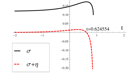
Figure 1: The solid (black) line represents the surface energy density $\sigma$, while the dashed (red) line denotes the quantity $\sigma+\eta$. When plotting these curves, we set $r_{\Sigma}=1,M=1,a_{0}=3,V_{0}=0.6,H=1.5$. At the moment $t=0.624554$, we have $\sigma+\eta=0$, $R_{\Sigma}=1.1756$, and $R_{UH}=1.24387$.

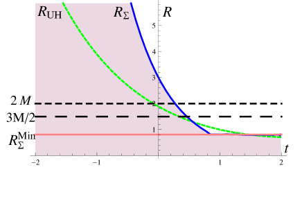
Figure 2: Universal horizon $R_{UH}$, the surface radius $R_{\Sigma}$ of the collapsing star vs $t$ for $r_{\Sigma}=1,M=1,a_{0}=3,V_{0}=0.6,H=1.5$. The horizontal lines $R=2M$ and $R=3M/2$ are, respectively, the Killing and universal horizons of the Schwarzschild vacuum solution. The collapse ends at the moment when $R_{\Sigma}=R^{Min}_{\Sigma}$, at which point the pressure of the surface of the collapsing star becomes infinitely large, whereby a space-time singularity with finite thickness is developed.

Figure 3: Gravitational collapse of a spherically symmetric star with its radius $R_{\Sigma}(t)$, which divides the space-time into two regions, $V^{\pm}$. The curved line $R_{UH}$ denotes the universal horizon formed inside the star, while the vertical straight line $R=3M/2$ is the universal horizon of the Schwarzschild vacuum solution. When the star collapses inside the Schwarzschild universal horizon $R=3M/2$, the universal horizon suddenly jumps from $R_{UH}(t_{o})$ to $3M/2$, because of the non-zero mass of the collapsing surface of the star.

Figure 4: Penrose diagram of a collapsing star described in the content for the case where the free parameters of the solution are chosen as $r_{\Sigma}=1,M=1,a_{0}=3,V_{0}=0.6,H=1.5$. The surface $\Sigma$ of the collapsing star divides the whole space-time into two regions, the external region $V^{+}$ and the internal region $V^{-}$. The curved line $UH$ denotes the universal horizon, while the straight line $EH$ the event horizon. The star collapses to form generically a space-time singularity at a finite non-zero radius $R=R^{Min}_{\Sigma}>0$.

IV Conclusions

In this paper, we have first generalized the definition of a stationary universal horizon to a dynamical one, by simply replacing Killing horizons by apparent ones. Then, we have constructed an analytical model that represents the gravitational collapse of a spherical symmetric star with finite thickness, and shown explicitly that dynamical universal horizons can be formed from such a “realistic” gravitational collapse. Here “realistic” is referred to as a gravitational collapse of a star with a finite thickness that satisfies at least the weak energy condition HE73 .

To have the problem tractable, we have assumed that the star consists of an anisotropic and homogeneous perfect fluid and that outside the star the space-time is vacuum in the framework of the Einstein-aether theory EA . When the effects of the aether field is negligible, the vacuum space-time is uniquely described by the Schwarzschild solution EA . Even in this case, solving the khronon equation (2.9) inside the star is still very complicated. Instead, we have further assumed that the velocity of the the khronon is infinitely large, so the sound horizon of the khronon coincides with the universal horizon. Then, we have found that an analytical solution exists for the star made of the de Sitter universe, and shown explicitly how a dynamical universal horizon can be formed, as can be seen from Figs. 2 - 4.

Although such a constructed model serves our current purpose very well, that is, to show that universal horizons can be indeed formed from realistic gravitational collapse, it would be very interesting to consider cases without (some of) the above assumptions, specially the case in which the space-time outside of the star is not vacuum, so that the star may radiate, when it is collapsing.

In addition, although in this paper we have considered the formation of the universal horizons only in the framework of the Einstein-aether theory, it is expected that our main conclusions should be true in other theories of gravity with broken LI, including the HL gravity ZWWS ; BPS .

References

- (1) A. Kostelecky and N. Russell, Rev. Mod. Phys. 83 11 (2011) [arXiv:0801.0287v7, January 2014 Edition].
- (2) D. Mattingly, Living Rev. Relativity, 8, 5 (2005); S. Liberati, Class. Qnatum Grav. 30, 133001 (2013).
- (3) K. Lin, E. Abdalla, R.-G. Cai, and A. Wang, Inter. J. Mod. Phys. D23, 1443004 (2014); K. Lin, F.-W. Shu, A. Wang, and Q. Wu, Phys. Rev. Din press (2015) [arXiv:1404.3413].
- (4) S. Carlip, Quantum Gravity in 2+1 Dimensions, Cambridge Monographs on Mathematical Physics (Cambridge University Press, Cambridge, 2003); C. Kiefer, Quantum Gravity (Oxford Science Publications, Oxford University Press, 2007).
- (5) P. Hořava, J. High Energy Phys. 0903, 020 (2009); Phys. Rev. D79, 084008 (2009).
- (6) E.M. Lifshitz, Zh. Eksp. Toer. Fiz. 11, 255 (1941); ibid., 11, 269 (1941).
- (7) M. Visser, Phys. Rev. D80, 025011 (2009); Power-counting renormalizability of generalized Hořava gravity, arXiv:0912.4757.
- (8) K.S. Stelle, Phys. Rev. D16, 953 (1977).
- (9) J. Collins, A. Perez, D. Sudarsky, L. Urrutia, and H. Vucetich, Phys. Rev. Lett. 93, 191301 (2004).
- (10) M. Pospelov and C. Tamarit, J. High Energy Phys. 01 (2014) 048.
- (11) T. Zhu, Q. Wu, A. Wang, and F.-W. Shu, Phys. Rev. D84, 101502(R) (2011); T. Zhu, F.-W. Shu, Q. Wu, and A. Wang, Phys. Rev. D85, 044053 (2012).
- (12) K. Lin, S. Mukohyama, A. Wang, and T. Zhu, Phys. Rev. D89, 084022 (2014).
- (13) C.M. Will, The Confrontation between General Relativity and Experiment, Living Rev. Relativity, 9, 3 (2006) [http://www.livingreviews.org/lrr-2006-3; arXiv:gr-qc/0510072].
- (14) T. Zhu, Y.-Q. Huang, and A. Wang, Phys. Rev. D87, 084041 (2013); A. Wang, Q. Wu, W. Zhao, and T. Zhu, Phys. Rev. D87, 103512 (2013); T. Zhu, W. Zhao, Y.-Q. Huang, A. Wang, and Q. Wu, Phys. Rev. D88, 063508 (2013).
- (15) E. Komatsu, et al., Astrophys. J. Suppl. 192, 18 (2011); P. Ade et al., Planck Collaboration, Astron. Astrophys., (2014).
- (16) S. Janiszewski and A. Karch, JHEP, 02, 123 (2013); Phys. Rev. Lett. 110, 081601 (2013).
- (17) D. Blas, O. Pujolas, and S. Sibiryakov, Phys. Lett. B688, 350 (2010); J. High Energy Phys. 1104, 018 (2011).
- (18) T. Jacobson and Mattingly, Phys. Rev. D64, 024028 (2001); T. Jacobson, Proc. Sci. QG-PH, 020 (2007).
- (19) T. Jacobson, Phys. Rev. D81, 101502 (R) (2010).
- (20) A. Wang, On “No-go theorem for slowly rotating black holes in Hořava-Lifshitz gravity, arXiv:1212.1040.
- (21) K. Yagi, D. Blas, N. Yunes, and E. Barausse, Phys. Rev. Lett. 112, 161101 (2014); K. Yagi, D. Blas, E. Barausse, and N. Yunes, Phys. Rev. D89, 084067 (2014).
- (22) R. Narayan and J.E. MacClintock, Mon. Not. R. Astron. Soc., 419, L69 (2012).
- (23) D. Blas and S. Sibiryakov, Phys. Rev. D84, 124043 (2011).
- (24) E. Barausse, T. Jacobson, and T. Sotiriou, Phys. Rev. D83, 124043 (2011); B. Cropp, S. Liberati, and M. Visser, Class. Quantum Grav. 30, 125001 (2013); M. Saravani, N. Afshordi, and R.B. Mann, Phys. Rev. D89, 084029 (2014); S. Janiszewski, A. Karch, B. Robinson, and D. Sommer, JHEP 04, 163 (2014); C. Eling and Y. Oz, JHEP, 11, 067 (2014); T. Sotiriou, I. Vega, and D. Vernieri, Phys. Rev. D90, 044046 (2014); J. Bhattacharyya and D. Mattingly, “Universal horizons in maximally symmetric spaces,” arXiv:1408.6479.
- (25) P. Berglund, J. Bhattacharyya, and D. Mattingly, Phys. Rev. D85, 124019 (2012); Phys. Rev. Lett. 110, 071301 (2013).
- (26) K. Lin, O. Goldoni, M.F. da Silva, and A. Wang, Phys. Rev. D in press (2015) [arXiv:1410.6678].
- (27) B. Cropp, S. Liberati, A. Mohd, and M. Visser, Phys. Rev. D89, 064061 (2014).
- (28) S.W. Hawking, G.F.R. Ellis, The Large Scale Structure of Spacetime (Cambridge University Press, Cambridge, 1973).
- (29) S.A. Hayward, Phys. Rev. D49, 6467 (1994); Class. Quantum Grav. 17, 1749 (2000).
- (30) A. Wang, Phys. Rev. D68, 064006 (2003); Phys. Rev. D72, 108501 (2005); Gen. Relativ. Grav. 37, 1919 (2005); Y. Wu, M.F.A. da Silva, N.O. Santos, and A. Wang, Phys. Rev. D68, 084012 (2003); A.Y. Miguelote, N.A. Tomimura, and A. Wang, Gen. Relativ. Grav. 36, 1883 (2004); P. Sharma, A. Tziolas, A. Wang, and Z.-C. Wu, Inter. J. Mord. Phys. A26, 273 (2011).
- (31) W. Israel, Nuovo Cimento, B 44 (1966) 1; B 48 (1967) 463 (E); A. Wang and N.O. Santos, Inter. J. Mod. Phys. A25, 1661 (2010).
- (32) W.B. Bonnor, A.K.G. de Oliveira, and N.O. Santos, Phys. Rept. 181, 269 (1989).
- (33) L. Amendola and S. Tsujikawa, Dark Energy: Theory and Observations (Cambridge University Press, Cambridge, 2010).