First-light LBT nulling interferometric observations: warm exozodiacal dust resolved within a few AU of $\eta$ Crv

Abstract

We report on the first nulling interferometric observations with the Large Binocular Telescope Interferometer (LBTI), resolving the N’ band (9.81 - 12.41 $\mu$m) emission around the nearby main-sequence star $\eta$ Crv (F2V, 1-2 Gyr). The measured source null depth amounts to 4.40% $\pm$ 0.35% over a field-of-view of 140 mas in radius ($\sim$2.6 AU at the distance of $\eta$ Crv) and shows no significant variation over 35^∘ of sky rotation. This relatively low null is unexpected given the total disk to star flux ratio measured by Spitzer/IRS ($\sim$23% across the N’ band), suggesting that a significant fraction of the dust lies within the central nulled response of the LBTI (79 mas or 1.4 AU). Modeling of the warm disk shows that it cannot resemble a scaled version of the Solar zodiacal cloud, unless it is almost perpendicular to the outer disk imaged by Herschel. It is more likely that the inner and outer disks are coplanar and the warm dust is located at a distance of 0.5-1.0 AU, significantly closer than previously predicted by models of the IRS spectrum ($\sim$3 AU). The predicted disk sizes can be reconciled if the warm disk is not centrosymmetric, or if the dust particles are dominated by very small grains. Both possibilities hint that a recent collision has produced much of the dust. Finally, we discuss the implications for the presence of dust at the distance where the insolation is the same as Earth’s (2.3 AU).

1 Introduction

The possible presence of dust in the habitable zones of nearby main-sequence stars is considered a major threat for the direct imaging and characterization of Earth-like extrasolar planets (exo-Earths) with future dedicated space-based telescopes. Several independent studies have addressed this issue and concluded that visible to mid-infrared direct detection of exo-Earths would be seriously hampered in the presence of dust disks 10 to 20 times brighter than the Solar zodiacal cloud assuming a smooth brightness distribution (e.g., Beichman et al., 2006b; Defrère et al., 2010; Roberge et al., 2012). The prevalence of exozodiacal dust at such a level in the terrestrial planet region of nearby planetary systems is currently poorly constrained and must be determined to design these future space-based instruments. So far, only the bright end of the exozodi luminosity function has been measured on a statistically meaningful sample of stars (Lawler et al., 2009; Kennedy & Wyatt, 2013). Based on WISE observations and extrapolating over many orders of magnitude, Kennedy & Wyatt (2013) suggest that at least 10% of Gyr-old main-sequence stars may have sufficient exozodiacal dust to cause problems for future exo-Earth imaging missions. To determine the prevalence of exozodiacal dust at the faint end of the luminosity function, NASA has funded the Keck Interferometer Nuller (KIN) and the Large Binocular Telescope Interferometer (LBTI) to carry out surveys of nearby main sequence stars. Science observations with the KIN started in 2008 and the results were reported recently (Millan-Gabet et al., 2011; Mennesson et al., in press). One of their analyses focused on a sample of 20 solar-type stars with no far infrared excess previously detected (i.e, no outer dust reservoir). Assuming a log-normal luminosity distribution, they derived the median level of exozodiacal dust around such stars to be below 60 times the solar value with high confidence (95%). Yet, the state-of-the-art exozodi sensitivity achieved per object by the KIN is approximately one order of magnitude larger than that required to prepare future exo-Earth imaging instruments.

The LBTI is the next step. A survey, called the Hunt for Observable Signatures of Terrestrial Planetary Systems (HOSTS, Hinz, 2013; Danchi et al., 2014), will be carried out on 50 to 60 carefully chosen nearby main-sequence stars over the next 4 years (Weinberger et al. in prep). In this paper, we report on the first mid-infrared nulling interferometric observations with the LBTI obtained on 2014 February 12 as part of LBTI’s commissioning. We observed the nearby main-sequence star $\eta$ Crv (F2V, 1.4 M_⊙, 18.3 pc), previously known to harbor unusually high levels of circumstellar dust. The infrared excess was first detected with IRAS (Stencel & Backman, 1991) and confirmed later by Spitzer/MIPS at 70 $\mu$m (Beichman et al., 2006a), Spitzer/IRS at 5 – 35 $\mu$m (Chen et al., 2006; Lisse et al., 2012), and Herschel at 70 – 500 $\mu$m (Duchêne et al., 2014). Interestingly, the SED exhibits two distinct peaks which can be explained by the presence of two well separated dust belts. The cold outer one was first resolved in the submillimeter and found to lie at a distance of $\sim$150 AU from the star Wyatt et al. (2005). Mid-infrared interferometric observations with VLTI/MIDI and the KIN resolved the inner belt to be located within 3 AU of the host star Smith et al. (2008, 2009); Millan-Gabet et al. (2011), a conclusion supported by blackbody models that place the warm dust near 1 AU (e.g., Wyatt et al., 2005). A detailed analysis of the dust composition in the inner belt using the Spitzer/IRS spectrum suggests a location nearer to 3 AU due to the presence of grains as small as 1 $\mu$m that are warmer than blackbodies for the same stellocentric distance (Lisse et al., 2012). Most importantly, the mid-infrared excess emission is remarkably large and intriguing considering the old age of the system (1-2 Gyr, Ibukiyama & Arimoto, 2002; Mallik et al., 2003; Vican, 2012) and all the aforementioned studies agree that it cannot be explained by mere transport of grains from the outer belt (at least not without a contrived set of planetary system parameters, Bonsor et al., 2012). This rather supports a rare and more violent recent event (e.g., Gáspár et al., 2013) and makes $\eta$ Crv an ideal object to study catastrophic events like the Late Heavy Bombardment that might have happened in the early solar system (Gomes et al., 2005) or a recent collision between planetesimals (e.g., as postulated for BD +20307, Song et al., 2005).

2 Observations and data reduction

2.1 Instrumental setup

The Large Binocular Telescope consists of a two 8.4-m aperture optical telescopes on a single ALT-AZ mount installed on Mount Graham in southeastern Arizona (at an elevation of 3192 meters) and operated by an international collaboration among institutions in the United States, Italy, and Germany (Hill et al., 2014; Veillet et al., 2014). Both telescopes are equipped with deformable secondary mirrors which are driven with the LBT’s adaptive optics system to correct atmospheric turbulence at 1 kHz (Esposito et al., 2010; Bailey et al., 2014). Each deformable mirror uses 672 actuators that routinely correct 400 modes and provide Strehl ratios exceeding 80%, 95%, and 99% at 1.6 $\mu$m, 3.8 $\mu$m, and 10 $\mu$m, respectively (Esposito et al., 2012; Skemer et al., 2014). The LBTI is an interferometric instrument designed to coherently combine the beams from the two 8.4-m primary mirrors of the LBT for high-angular resolution imaging at infrared wavelengths (1.5-13 $\mu$m, Hinz et al., 2012). It is developed and operated by the University of Arizona and based on the heritage of the Bracewell Infrared Nulling Cryostat on the MMT (BLINC, Hinz et al., 2000). The overall LBTI system architecture and performance will be presented in full detail in a forthcoming publication (Hinz et al. in prep). In brief, the LBTI consists of a universal beam combiner (UBC) located at the bent center Gregorian focal station and a cryogenic Nulling Infrared Camera (NIC). The UBC provides a combined focal plane for the two LBT apertures while the precise overlapping of the beams is done in the NIC cryostat. Nulling interferometry, a technique proposed 36 years ago to image extra-solar planets (Bracewell, 1978), is used to suppress the stellar light and improve the dynamic range of the observations. The basic principle is to combine the beams in phase opposition in order to strongly reduce the on-axis stellar light while transmitting the flux of off-axis sources located at angular spacings which are odd multiples of 0.5$\lambda/B$ (where $B=14.4$ m is the distance between the telescope centers and $\lambda$ is the wavelength of observation). Beam combination is done in the pupil plane on a 50/50 beamsplitter which can be translated to equalize the pathlengths between the two sides of the interferometer. One output of the interferometer is reflected on a short-pass dichroic and focused on the NOMIC camera (Nulling Optimized Mid-Infrared Camera, Hoffmann et al., 2014). NOMIC uses a 1024x1024 Raytheon Aquarius detector split into 2 columns of 8 contiguous channels. The optics provides a field of view (FOV) of 12 arcsecs with a plate-scale of 0.018 arcsecs. Tip/tilt and phase variations between the LBT apertures are measured using a fast-readout (1 Hz) K-band PICNIC detector (PHASECam) which receives the near-infrared light from both outputs of the interferometer. Closed-loop correction uses a fast pathlength corrector installed in the UBC (see more details in Defrère et al. 2014).

2.2 Observations

Nulling interferometric observations of $\eta$ Crv were obtained in the N’ band (9.81 - 12.41 $\mu$m) on 2014 February 12 as part of LBTI’s commissioning. The basic observing block (OB) consisted of one thousand frames, each having an integration time of 85 ms, for a total acquisition time of 110 seconds including camera overheads. The observing sequence was composed of several successive OBs at null, i.e. with the beams from both telescopes coherently overlapped in phase opposition, and one OB of photometric measurements with the beams separated on the detector. In order to estimate and subtract the mid-IR background, the OBs at null were acquired in two telescope nod positions separated by 2$\farcs$3 on the detector. We acquired 3 different observations of $\eta$ Crv interleaved with 4 observations of reference stars to measure and calibrate the instrumental null floor (CAL1-SCI-CAL2-SCI-CAL1-SCI-CAL3 sequence; see target and calibrator information in Table 1). To minimize systematic errors, calibrator targets were chosen close to the science target, both in terms of sky position and magnitude, using the SearchCal software (Bonneau et al., 2011). The 7 observations occurred over a period of approximately 3 hours around the meridian transit (see u-v plane covered by the science observations in Fig. 1) with relatively stable weather conditions. The seeing was $\sim$1$\farcs$4 for the first observation and 1$\farcs$0-1$\farcs$2 for the remainder observations. The adaptive optics systems (AO) were locked with 300 modes (left side) and 400 modes (right side) at a frequency of 990 Hz over the duration of the observations. Fringe tracking was carried out at 1kHz using a K-band image of pupil fringes and an approach equivalent to group delay tracking (Defrère et al., 2014). The phase setpoint was optimized at least once per observation to take out any optical path variation between the K-band, where the phase is measured and tracked, and the N’-band, where the null depth is measured (making sure that the phase maintained at K-band provided the best possible nulls at N’ band). The NOMIC detector was used with the small well depth for better sensitivity and in subframe mode (512$\times$512 pixels) to reduce the camera overhead.

Table 1: Basic properties of $\eta$ Crv and its calibrators.

ID	HD	RA-J2000	DEC-J2000	Type	$m_{V}$	$m_{K}$	$F_{\rm\nu,N^{\prime}}$	$\theta_{\rm LD}\pm 1\sigma$	Refs.
		[d m s]	[d m s]				[Jy]	[mas]
$\eta$ Crv	109085	12 32 04	-16 11 46	F2V	4.30	3.37	1.76	0.819 $\pm$ 0.119	A13
CAL 1	108522	12 28 02	-14 27 03	K4III	6.80	3.46	1.68	1.204 $\pm$ 0.016	M05
CAL 2	107418	12 20 56	-13 33 57	K0III	5.15	2.83	2.96	1.335 $\pm$ 0.092	B11
CAL 3	109272	12 33 34	-12 49 49	G8III	5.59	3.60	1.42	0.907 $\pm$ 0.063	B11

References. Coordinates, spectral types and V/K magnitudes from SIMBAD; N’-band flux densities computed by SED fit (Weinberger et al. in prep); Limb-darkened diameters and 1-$\sigma$ uncertainties from [A13] Absil et al. (2013), [M05] Mérand et al. (2005), and [B11] Bonneau et al. (2011).

2.3 Data reduction and calibration

Data reduction and calibration were performed using the nodrs pipeline developed by the LBTI and HOSTS teams for the survey (Defrère et al. in prep). It converts raw NOMIC frames to calibrated null measurements in five main steps: frame selection, background subtraction, stellar flux computation, null computation, and null calibration. Frame selection is done by removing the first 20 frames of each OB that are affected by a transient behavior of the NOMIC detector. Background subtraction is achieved by nod pairs, subtracting from each frame the median of frames recorded in the other nod position. Each row in a given channel is then corrected for low frequency noise (Hoffmann et al., 2014) by subtracting its sigma-clipped median, excluding the region around the star position. Remaining bad pixels were identified using the local standard deviation (5-$\sigma$ threshold) and replaced with the mean of the neighbor pixels. The flux computation is done in each frame by aperture photometry using an aperture radius of 8 pixels (140 mas or 2.6 AU at the distance of $\eta$ Crv), equivalent to the half width at half maximum (HWHM) of the single-aperture PSF at 11.1 $\mu$m. The background flux in the photometric aperture is estimated simultaneously in each frame using all pixels covering the same columns as the photometric region and located between the second minimum of the single-aperture PSF (34 pixels or 600 mas) and the channel edge. Raw null measurements are then obtained by dividing the individual flux measurements at null by the total flux estimated from the photometric OB of the same observation (accounting for the 50/50 beamsplitter). This procedure is performed exactly the same way for $\eta$ Crv and the three calibrators. Finally, in order to correct for the differential background error on the null due to the different brightness of the stars, we further add to the null a small fraction of background flux measured in a nearby empty region of the detector. This fraction is computed to match the background error on the null between the different stars, assuming fully uncorrelated noise in the photometric aperture and the nearby empty region of the detector (see Appendix A). To compute the final null value per OB, we first remove the outliers using a 5-$\sigma$ threshold and then perform the weighted-average of the lowest 5% null measurements (the weight being defined as the inverse square of the uncertainty in the aperture photometry). The corresponding null uncertainty is computed by bootstrapping through the entire dataset (keeping the lowest 5% each time) and taking the 16 and 84% levels from the cumulative distribution as representative 1-$\sigma$ uncertainties. A description of the additional systematic errors considered is given in Section 3. The raw null measurements per OB for $\eta$ Crv and its calibrators are shown in the top panel of Figure 1.

The instrumental null floor is estimated using the calibrator null measurements corrected for the finite extension of the stars. This correction is done using a linear limb-darkened model for the geometric stellar null (Absil et al., 2006):

$$N_{\rm star}=\left(\frac{\pi B\theta_{\rm LD}}{4\lambda}\right)^{2}\left(1-\frac{7u_{\lambda}}{15}\right)\left(1-\frac{u_{\lambda}}{3}\right)^{-1};\\$$ (1)

where $B$ is the interferometric baseline, $\theta_{\rm LD}$ is the limb-darkened angular diameter of the photosphere (see Table 1), $\lambda$ is the effective wavelength, and $u_{\lambda}$ is the linear limb-darkening coefficient. Given the relatively short interferometric baseline of the LBTI, the geometric stellar null will generally be small in the mid-infrared and the effect of limb-darkening negligible. Assuming $u_{\lambda}$ = 0, the typical geometric null for our targets is $\sim 10^{-5}$ with an error bar of $\sim 10^{-6}$, which is small compared to our measurement errors. The next step in the calibration is to compute the instrumental null floor at the time of the science observations and subtract it from the raw null measurements of the science target (null contributions are additive, Hanot et al., 2011). This can be estimated in various ways, using only bracketting calibrator measurements, a weighted combination of the calibrators, or by polynomial interpolation of all calibrator measurements. In the present case, because $\eta$ Crv and its calibrators have been chosen close in magnitude and position on the sky, we assume that the instrument behaved consistently for the duration of the observations and use a single/constant to fit the instrumental null floor, as shown by the solid line in the top panel of Figure 1. The only noticeable difference between $\eta$ Crv (F2V) and its calibrators (G8III to K4III) is the spectral type but the slope of the stellar flux across the N’ band is the same so there is no differential chromatic bias on the null measurement.

The statistical uncertainty on a calibrated null measurement is computed as the quadratic sum of its own statistical uncertainty and the statistical uncertainty on the null floor measured locally at any given time by using the 1-$\sigma$ variation on the constant fit of the instrumental null floor. The systematic uncertainty, on the other hand, is computed globally and is composed of two terms. The first one accounts for the uncertainty on the stellar angular diameters, taking the correlation between calibrators into account. As described above, it is negligible in this case. The second one is computed as the weighted standard deviation of all calibrator measurements and accounts for all other systematic uncertainties, which are harder to estimate on a single-OB basis (see Section 3). The statistical and systematic uncertainties are uncorrelated and added quadratically to give the total uncertainty on a calibrated null measurement. The part of this uncertainty related to the the null floor is represented by the dashed lines in the top panel of Figure 1. The calibrated null measurements are shown in Section 5.

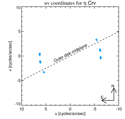
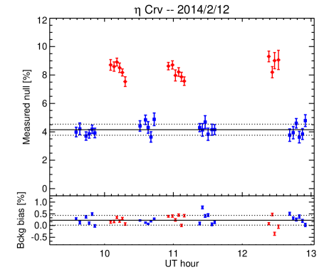
Figure 1: Left, sampling of the Fourier (u,v) plane obtained for $\eta$ Crv on 2014 February 12. Each blue point and its centrosymmetric counterpart represent the orientation of the LBTI baseline for a given OB. The orientation of the outer disk midplane (i.e., 116$\fdg$3, Duchêne et al., 2014) is represented by the black dashed line. The right figure shows the corresponding raw null measurements per OB as a function of UT time (top panel). The blue squares show the calibrator measurements while the red diamonds represent the $\eta$ Crv measurements. The estimated instrumental null floor is represented by the solid black line and the corresponding 1-$\sigma$ uncertainty by the dotted lines. The bottom panel shows the corresponding background error estimate measured in a nearby empty region of the detector.

3 Data analysis and results

Figure 1 shows that the null measurements obtained on the science target (red diamonds) are clearly above the instrumental null floor (blue squares), suggestive of resolved emission around $\eta$ Crv. In order to quantify the measured excess emission, the first step of the data analysis is to convert the calibrated null measurements into a single value. Given that the calibrated null measurements show no significant variation as a function of the baseline rotation, this is done by computing the weighted average of all calibrated null measurements and gives $4.40\%\pm 0.10\%\pm 0.34\%$, where the two uncertainty terms correspond to the statistical and the systematic uncertainties respectively. The statistical uncertainty decreases with the number of data points and is computed as follows:

$$\sigma_{\rm stat}=\frac{1}{\sqrt{\sum_{i}1/\sigma^{2}_{i,\rm stat}}};\\$$ (2)

where $\sigma_{i,\rm stat}$ is the statistical part of the uncertainty on the $i$th calibrated data point. The systematic uncertainty on the other hand has been computed globally and we make here the conservative assumption that it is fully correlated between all data points. The systematic uncertainty on the final calibrated null is hence given by the systematic uncertainty on the null floor, which is the same for all calibrated data points. Several instrumental imperfections contribute to this uncertainty. First, there is a background measurement bias between the photometric aperture and the nearby regions used for simultaneous background measurement and subtraction. The amplitude of this bias depends on the the photometric stability (i.e., precipitable water vapor, temperature, clouds) and the nodding frequency. It was estimated using various empty regions of the detector located around the photometric aperture. The result is shown for one representative empty region in the bottom panel of Figure 1 and accounts for 0.18% of the systematic uncertainty. Another main contributor to the systematic uncertainty comes from the mean phase setpoint used to track the fringes. Using a more advanced data reduction technique (i.e., Hanot et al., 2011) on similar data sets, we estimate that this error can produce a null uncertainty as large as 0.2% between different OBs. Finally, a variable intensity mismatch between the two beams can also impair the null floor stability. In the present case, it was measured in each observation using the photometric OBs and found to be stable at the 1.5% level, corresponding to a null error of $\sim$0.1%. Adding quadratically these 3 terms gives a systematic uncertainty of 0.29%, similar to the value found after data reduction (i.e., 0.34%).

The final step of the data analysis is to compute the fraction of the calibrated source null depth that actually comes from the circumstellar environment by subtracting the null depth expected from the stellar photosphere alone. Using a limb-darkened diameter of 0.819 $\pm$ 0.119 mas (see Table 1) and Equation 1, the stellar contribution to the total null depth is 0.0014% $\pm$ 0.0004% which is negligible compared to the calibrated null excess. Therefore, adding quadratically the statistical and systematic uncertainties, the final source null depth detected around $\eta$ Crv is 4.40% $\pm$ 0.35%. To make sure that no dust emission is lying outside the photometric aperture, we reduced the data using larger apertures and following exactly the same procedure. The results are illustrated in Figure 2 for four different aperture radii which are multiple of the half width at half maximum of the single-aperture PSF at 11.1 $\mu$m. The lack of significant increase in the null measurements for larger aperture radii suggests that the angular size of the inner disk is smaller than the size of the single-aperture PSF (2.6 AU in radius). This result is in agreement with the conclusion from single-dish imaging (Smith et al., 2008) and the KIN (Mennesson et al., in press).

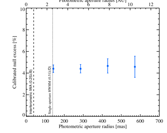
Figure 2: Calibrated null excess as a function of photometric aperture radius. The left vertical dashed line indicates the interferometric inner working angle (i.e., $\lambda/4B$=39 mas or 0.7 AU at the distance of $\eta$ Crv) while the right vertical dotted line represents the default aperture radius used in this study (i.e., the half width at half maximum of the single-aperture PSF at 11.1 $\mu$m). The lack of significant increase in the null measurements for larger aperture radii suggests that the regions emitting the majority of the N’-band flux is more compact than the size of the single-aperture PSF.

4 Modeling and interpretation

A first step toward interpreting the calibrated null depth observed for $\eta$ Crv can be made simply by comparing it with the ratio of disk to photospheric flux observed with Spitzer/IRS. Using the spectrum presented in Lebreton et al. (in prep) and assuming an absolute calibration error of 3%, we derive a value of 22.7% $\pm$ 5.4% over the N’ band. This is a very conservative uncertainty estimate which is consistent with previous studies (Chen et al., 2006; Lisse et al., 2012). For any centrosymmetric disk, approximately half the disk flux is transmitted through the LBTI fringe pattern unless the extent of the N’-band emission is comparable to, or smaller than the angular resolution of the interferometer (i.e., $\lambda/2B$=79 mas or 1.4 AU). The observed null depth of 4.40% $\pm$ 0.35%, i.e. substantially lower than the disk to star flux ratio, suggests therefore that the disk is either compact or edge-on with a position angle perpendicular to the LBTI baseline. An edge-on disk perpendicular to the baseline would have a position angle of around 0-20^∘ which is specifically disfavored by VLTI/MIDI observations (see Fig. 11 in Smith et al., 2009). In addition, the inner disk would be nearly perpendicular to the outer disk plane whose orientation has been consistently measured by independent studies (see dashed line in Figure 1, Wyatt et al., 2005; Duchêne et al., 2014; Lebreton et al., in prep). Given that the warm dust may be scattered in from the cool outer belt (e.g., Wyatt et al., 2007; Lisse et al., 2012), such a configuration seems unlikely and would be difficult to explain dynamically. Besides, among the planetary systems with measured inner and outer disk orientations (e.g., Solar system, $\beta$ Pic, AU Mic), none shows perpendicular inner and outer disks. A more likely scenario is for the inner and outer disk components to be coplanar, and to concentrate more than half the disk flux within 1.4 AU.

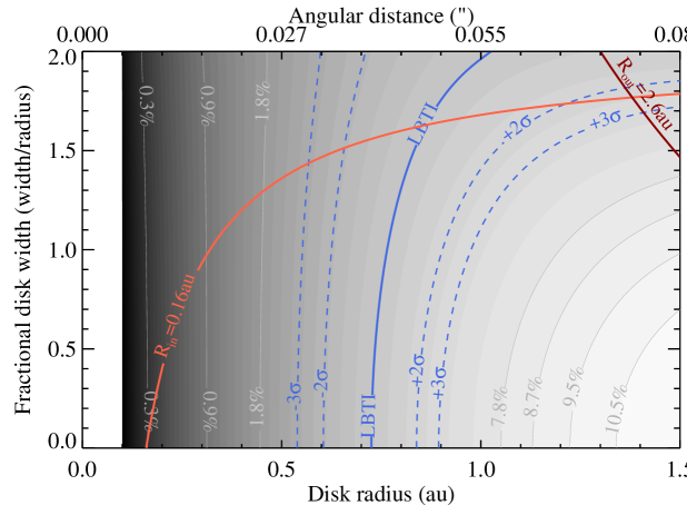
Figure 3: Constraints on the location and width of the resolved excess emission detected around $\eta$ Crv. Grey contours and labels show the predicted LBTI null assuming a disk to star flux ratio of $\sim$23% and the same orientation as the outer belt. Blue lines show the observed LBTI null and corresponding uncertainties. The left red line shows the inner disk radius lower limit of 0.16 AU as derived with VLTI/MIDI while the right dark red line indicates the outer limit set by our observations. Considering all constraints, the disk is restricted to lie at a distance of 0.5-1.0 AU, with a full width of up to 1.7 AU.

In order to interpret our observations within the context of a physical model, we construct a simple vertically thin model for the inner disk using the analytical tool developed by the HOSTS team (Kennedy et al., submitted to ApJ). As expected from the qualitative description above, scaled models of the Solar zodiacal cloud that match the observed total and transmitted disk fluxes have position angles near-perpendicular to the outer disk. That is, this model is too radially extended so, unless the inner disk is strongly misaligned with the outer disk, a scaled version of our Solar zodiacal cloud is not a good match to the warm disk around $\eta$ Crv. We therefore explore the alternative possibility that the inner and outer disks are coplanar. With the disk orientation fixed, it is necessary to vary the location and width of the warm dust disk to reproduce both the total disk flux and the calibrated null measured by LBTI. That is, the only free parameters are the disk radius and width ($r$ and $\delta r$), and the power-law for the dust (i.e., surface density or optical depth) between these radii ($\alpha$). The results of this process, for the radius and width, are shown in Figure 3. The greyscale and grey contours show the null depths of models with a range of radii $r$ and fractional widths $\delta r/r$, where in each case the total disk to star flux ratio is 23% in the N’ band (using $\alpha=0.34$). The null depths vary from near zero for small disk radii, to about 11% for narrow rings with $r\approx 1.5$ AU. The blue lines show where the predicted null depths agree with the LBTI observations of $\eta$ Crv with the range allowed by 2 and 3-$\sigma$ uncertainties. These uncertainties do not account for the 5% uncertainty in the Spitzer/IRS excess, which for example moves the blue lines systematically approximately 0.1 AU outward for a 5% lower excess. Similarly, if the IRS excess is larger, which is possible if the excess is present at shorter wavelengths (e.g., Lisse et al., 2012), then the disk lies even closer to the star. With these assumptions, the inner disk component is constrained to lie at approximately 0.5-1.0 AU with varying width.

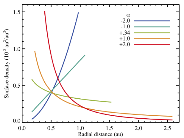
Figure 4: Surface density as a function of distance from the star for five disk models having different power-law indices $\alpha$. Each line represents the widest disk allowed in a Figure 3 computed for the corresponding $\alpha$. For a steeply decreasing surface density profile (i.e., large $\alpha$), the disk can extend beyond 1 AU but the disk emission is then more concentrated.

As noted in Section 3, the lack of increase in the null measurements for larger aperture radii suggests that the disk is smaller than 2.6 AU in radius. From MIDI, VISIR, and MICHELLE observations, Smith et al. (2009) constrain the inner disk to lie outside 0.16 AU. These constraints are shown by the red curves in Figure 3, and serve as useful limits if the disk is wide, in which case the LBTI does not constrain the disk extent strongly. The constraint is in fact better than appears from Figure 3 because even the widest models are concentrated; half of the total disk flux originates from within 0.8 AU. Wide disks are only allowed because enough of their emission is blocked by the LBTI transmission pattern so the qualitative description given above holds. The zoo of possible models can be made even larger by adjusting the surface density power law. The default value of $\alpha$=0.34 used above comes from the solar Zodiacal cloud model (Kelsall et al., 1998) which is not necessarily a good match to the warm disk around $\eta$ Crv. It could be very different depending on the physical origin of the disk, and depends on dynamical, collisional, and radiation processes. Given that the warm dust around $\eta$ Crv may be scattered in from the cool outer belt (e.g., Wyatt et al., 2007; Lisse et al., 2012), predictions of the expected $\alpha$ would be highly uncertain. However, its value has a very weak impact on the warm dust location as shown in Figure 4. For models where the surface density increases with radius ($\alpha<0$), the disk emission is concentrated farther from the star, so the disk must be smaller in order to fit our data. If the disk surface density decreases with radius ($\alpha>0$), our ability to constrain the disk extent is limited. However, for these models most of the emission comes from the inner disk edge, so the inability to constrain the outer edge location is expected, and applies similarly to other observations. Therefore, regardless of the disk profile, the conclusion from any centrosymmetric model is that the bulk of the disk emission lies closer to the star than previously thought, most likely in the range 0.5-1 AU.

5 Discussion

The warm dust location derived in the previous section is significantly closer to the star than inferred from Spitzer/IRS spectrum models (3 AU or 160 mas, Lisse et al., 2012). There is however significant uncertainty in this inference because it relies on complex grain models with degenerate parameters. While the LBTI observations clearly suggest that these models need to be revisited, an alternative scenario to reconcile the difference in the inferred disk sizes is to relax the assumption of a centrosymmetric disk. If the inner disk has an over-density that was hidden behind a transmission minimum for the range of observed hour angles, then the disk can be larger and may still satisfy the observed LBTI null and Spitzer/IRS excess (i.e., a clump can be at larger physical separation, but remain close to the star in sky-projected distance). Future observations can therefore aim to expand the range of hour angles and also look for significant variations in the calibrated null depth at the same hour angles. Such observations will help establish whether an asymmetry exists, and if so, whether that asymmetry is orbiting the star or fixed in space. The latter possibility would favor recent collision scenarios which suggest that a long-lasting asymmetry is created at the location where the impact occurred (Jackson et al., 2014).

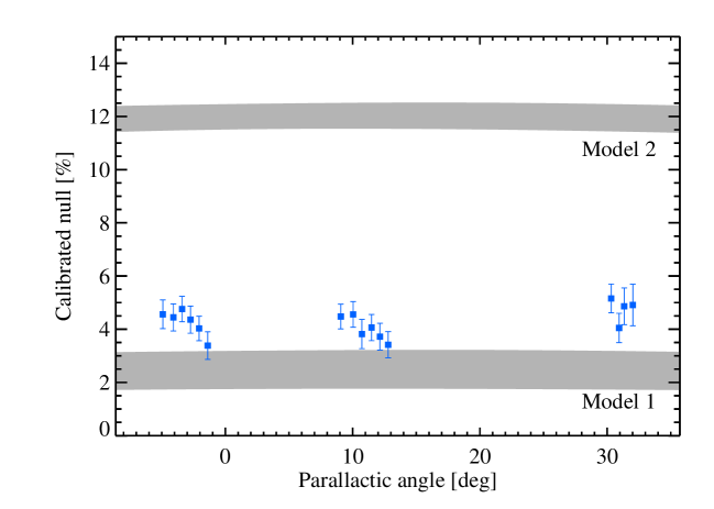
Figure 5: Calibrated null measurements as a function of parallactic angle for our LBTI observations of $\eta$ Crv (February 12, 2014). The null expected from the two best-fit exozodiacal disk models derived by Lebreton et al. (in prep) to reconcile the KIN observations with the shape of the Spitzer/IRS spectrum are shown by the grey-shaded areas (see main text for model description). The width of the grey-shaded areas is set by the uncertainty on the density peak location of the model.

New modeling based on Spitzer/IRS models and KIN observations also suggests a compact warm disk emitting mostly from within 1 AU (Lebreton et al., in prep). Using the GraTer radiative transfer modeling code (Augereau et al., 1999), Lebreton et al. (in prep) propose two inner disk models that reconcile the KIN observations with the shape of the mid-infrared Spitzer/IRS spectrum and various photometric constraints from IRAS, AKARI, WISE, and Spitzer/MIPS. The first model (model 1 hereafter) consists of small amorphous forsterite (Mg₂SiO₄, Jäger et al., 2003) dust grains with a differential size distribution defined by $n(a)\propto a^{-\kappa}$, with $\kappa=4.5$ and $a_{\rm min}=1.2~{}{\micron}$. The density peak location of the grains is 0.16-0.25 AU with a radial decrease in surface density $\propto r^{-1.5}$. Note that forsterite grains are also the dominant species in the Spitzer/IRS best-fit model of Lisse et al. (2012). The second model (model 2 hereafter) consists of astronomical silicates (Draine & Lee, 1984), with a minimum size of $a_{\rm min}=0.6~{}{\micron}$ and a size distribution slope of $\kappa=3.5$. The density peak location of the grains is 0.73-0.85 AU with an outer density slope of $-1$. The expected null excess for both models is shown in Figure 5 as a function of parallactic angle. As indicated by the grey-shaded areas, model 1 is a better fit to the LBTI observations, particularly for its larger value of the density peak position (0.25 AU). To understand how the LBTI observations break the model degeneracy, the two disk models are shown on top of the LBTI and KIN transmission maps in Figure 6. While both models logically produce a similar flux at the output of the KIN, the expected flux transmitted to the null output of the LBTI is significantly lower for model 1 due to the shorter nulling baseline and the small extent of the disk model. Approximately 10-19% of the disk flux is transmitted to the null output for model 1, depending on the density peak position (i.e., 0.16-0.25 AU), while this value reaches 48-51% for model 2 (0.73-0.85 AU). This explains the difference in the predicted null excess shown in Figure 5. While the parameters of model 1 could be tuned to better fit our observations, this analysis clearly shows that it is possible to reconcile the Spitzer/IRS model with spatial constraints from the KIN and the LBTI. The very steep size distribution and resulting large population of very small grains of such a model depart significantly from the behavior expected for a collisional cascade in equilibrium (Gáspár et al., 2012). It is possible that this is evidence for the dust being the product of a transient, high rate of collisions (e.g., Olofsson et al., 2012).

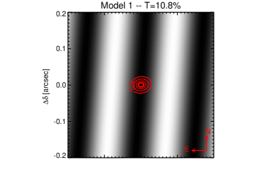
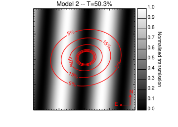
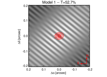
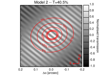
Figure 6: The two best-fit exozodiacal disk models derived by Lebreton et al. (in prep) to reconcile the KIN observations with the shape of the Spitzer/IRS spectrum shown on top of the sky transmission map of the LBTI (top row) and the KIN (bottom row). Model 1 is on the left and model 2 on the right (see main text for model descriptions). The contours mark regions corresponding to given ratios of the maximum disk flux density (see contour label), assuming that the inner warm disk has the same orientation as the outer disk imaged by Herschel (Duchêne et al., 2014). While the predicted flux transmitted through the KIN is logically similar for both models (see value in the upper left legend), it is significantly different in the case of the LBTI which is well matched for few AU-scale dust emission around near main-sequence stars and allows to break the degeneracy between the models (see Figure 5 for the corresponding expected null measurements). The LBTI sky transmission map is shown for the first OB of our observations (Julian date: 2456700.9204, parallactic angle: -4$\fdg$9, hour angle: -0h18). The KIN sky transmission map is shown for the same hour angle. North is up, East is to the left.

An important question related to the overall goal of LBTI is what the dust level in the habitable zone around $\eta$ Crv is. From the above discussion, it is clear that a scaled version of the Solar zodiacal dust cloud is not a good match to the observations and quoting a “zodi” level could therefore be confusing (see Roberge et al., 2012, for a discussion about this unit). To quantify the amount of warm dust, we can instead compare the surface density of our models with that of the Solar zodiacal cloud at the same equivalent position (i.e., scaled as $\sqrt{L_{\star}}$). Several possible scenarios have been discussed, and each will make different predictions. In the simplest scenario, where the inner disk is coplanar with the outer disk, the analytical model presented in Figure 3 has a surface density at 0.7 AU approximately 10⁴ times greater than that at the equivalent location in the Solar zodiacal cloud (i.e., 0.3 AU). At 2.3 AU, the distance where the insolation is the same as Earth’s at $\sqrt{L_{\star}}$, it has formally no dust since models within the 2-$\sigma$ contours in Figure 3 all have outer edges within 2 AU. The radiative transfer disk model (model 1) on the other hand is not truncated at its outer edge (surface density $\propto r^{-1.5}$) and has a surface density at 2.3 AU approximately 12000 times larger than that at 1 AU in the Solar zodiacal cloud. Finally, in the non-centrosymmetric scenarios, the possibility of even more dust at larger radii means that the habitable zone dust levels could be even larger, but localized to certain azimuthal ranges which would be a source of confusion for future imaging missions (e.g., Defrère et al., 2012). Even if the lack of variation of the null measurements as a function of the observed baseline position angle suggests that the disk is most likely centrosymmetric, this scenario cannot be ruled out with the present data and more observations expanding the range of sky rotation are required.

6 Summary and conclusions

This paper presents the first science results from the LBTI nuller, a mid-infrared interferometric instrument combining the two 8.4-m apertures of the LBT. As part of LBTI’s commissioning observations, we observed the nearby main-sequence star $\eta$ Crv, previously known to harbor high levels of circumstellar dust. The data are consistent with a source null depth of 4.40% $\pm$ 0.35% across the N’ band (9.81 - 12.41 $\mu$m) and over a field-of-view of 140 mas in radius ($\sim$2.6 AU at the distance of $\eta$ Crv). The measured null shows no significant variation over 35^∘ of sky rotation and is relatively low compared to the total disk to star flux ratio of 23% observed with Spitzer/IRS, suggesting that a significant fraction of the dust lies within the central nulled response of the LBTI (79 mas or 1.4 AU along the baseline orientation). Assuming that the inner and outer disk components are coplanar, we show that the bulk of the warm dust emission must lie at a distance of 0.5-1.0 AU from the star in order to fit our data. This is consistent with spatial constraints from the KIN that also point toward a compact warm disk emitting mostly from within 1 AU but significantly closer than the distance predicted by the Spitzer/IRS spectrum models (3 AU). This discrepancy illustrates how spatially resolved observations provide crucial information to break the degeneracy inherent to SED-based modeling of proto-planetary and debris disks showing evidence of warm emission. This is discussed in detail for $\eta$ Crv in a companion paper based on the KIN observations (Lebreton et al., in prep). In this paper, we show how the LBTI observations break the degeneracy between models that have the same SEDs and KIN nulls and discuss an alternative scenario which is the possible presence of an over-density in the inner disk. Both scenarios support the prevailing interpretation for the origin of the warm dust which is a recent collision in the inner planetary system. To conclude, it is clear that $\eta$ Crv is not a good target for a future exo-Earth imaging mission since the surface density of the dust in or near the habitable zone can be as high as four orders of magnitude larger than that in the Solar zodiacal cloud.

Appendix A Correcting the background bias between stars of different magnitudes

The best 5% approach used in this paper to convert a series of individual null measurements to a single value creates a bias between stars of different magnitudes. The origin of this bias is the background noise which is presumably constant in absolute flux and divided by the flux of the star to compute the null. Therefore, the width of the relative background flux distribution decreases with the brightness of the star and the mean of the best 5% measurements increases. The contribution of the background noise to the measured null then creates a bias that depends on the brightness of the star. In order to compensate for this effect, we can add a small fraction of background flux to the measured flux at null to match the relative background noise on stars of different magnitudes. Explicitly, we are looking for the fraction $x$ verifying the following equation:

$${\rm variance}\left(\frac{B_{2}(t)}{F_{2}}\right)={\rm variance}\left(\frac{B_{1}(t)}{F_{1}}+xB(t)\right)$$ (A1)

where $F_{1}$ and $F_{2}$ are the stellar fluxes measured in the photometric OBs (assuming $F_{1}>F_{2}$), $B_{1}(t)$ and $B_{2}(t)$ are the instantaneous background fluxes in the photometric aperture in the null OBs, and $B(t)$ is the instantaneous background flux measured in a nearby empty region of the detector. Assuming that $B_{1}(t)$ and $B(t)$ are uncorrelated, their variance adds up and the above equation becomes:

$$\frac{1}{F_{2}^{2}}=\frac{1}{F_{1}^{2}}+x^{2}{\,\,\,\,\Rightarrow\,\,\,\,}x=\frac{\sqrt{F_{1}^{2}-F_{2}^{2}}}{F_{1}F_{2}},\,\\$$ (A2)

where we have assumed that $\sigma_{B_{1}}$= $\sigma_{B_{2}}$= $\sigma_{B}$.

References

- Absil et al. (2006) Absil, O., den Hartog, R., Gondoin, P., et al. 2006, A&A, 448, 787
- Absil et al. (2013) Absil, O., Defrère, D., Coudé du Foresto, V., et al. 2013, A&A, 555, A104
- Augereau et al. (1999) Augereau, J. C., Lagrange, A. M., Mouillet, D., Papaloizou, J. C. B., & Grorod, P. A. 1999, A&A, 348, 557
- Bailey et al. (2014) Bailey, V. P., Hinz, P. M., Puglisi, A. T., et al. 2014, in Society of Photo-Optical Instrumentation Engineers (SPIE) Conference Series, Vol. 9148, Society of Photo-Optical Instrumentation Engineers (SPIE) Conference Series, 3
- Beichman et al. (2006a) Beichman, C., Lawson, P., Lay, O., et al. 2006a, in Proc. SPIE, Vol. 6268
- Beichman et al. (2006b) Beichman, C. A., Bryden, G., Stapelfeldt, K. R., et al. 2006b, ApJ, 652, 1674
- Bonneau et al. (2011) Bonneau, D., Delfosse, X., Mourard, D., et al. 2011, A&A, 535, A53
- Bonsor et al. (2012) Bonsor, A., Augereau, J.-C., & Thébault, P. 2012, A&A, 548, A104
- Bracewell (1978) Bracewell, R. N. 1978, Nature, 274, 780
- Chen et al. (2006) Chen, C. H., Sargent, B. A., Bohac, C., et al. 2006, ApJS, 166, 351
- Danchi et al. (2014) Danchi, W., Bailey, V., Bryden, G., et al. 2014, in Proc. SPIE, Vol. 9146
- Defrère et al. (2010) Defrère, D., Absil, O., den Hartog, R., Hanot, C., & Stark, C. 2010, A&A, 509, A9+
- Defrère et al. (2012) Defrère, D., Stark, C., Cahoy, K., & Beerer, I. 2012, in Society of Photo-Optical Instrumentation Engineers (SPIE) Conference Series, Vol. 8442, Society of Photo-Optical Instrumentation Engineers (SPIE) Conference Series, 0
- Defrère et al. (2014) Defrère, D., Hinz, P., Downey, E., et al. 2014, in , 914609–914609–8
- Draine & Lee (1984) Draine, B. T., & Lee, H. M. 1984, ApJ, 285, 89
- Duchêne et al. (2014) Duchêne, G., Arriaga, P., Wyatt, M., et al. 2014, ApJ, 784, 148
- Esposito et al. (2010) Esposito, S., Riccardi, A., Quirós-Pacheco, F., et al. 2010, Appl. Opt., 49, G174
- Esposito et al. (2012) Esposito, S., Riccardi, A., Pinna, E., et al. 2012, in Society of Photo-Optical Instrumentation Engineers (SPIE) Conference Series, Vol. 8447, Society of Photo-Optical Instrumentation Engineers (SPIE) Conference Series
- Gáspár et al. (2012) Gáspár, A., Psaltis, D., Rieke, G. H., & Özel, F. 2012, ApJ, 754, 74
- Gáspár et al. (2013) Gáspár, A., Rieke, G. H., & Balog, Z. 2013, ApJ, 768, 25
- Gomes et al. (2005) Gomes, R., Levison, H. F., Tsiganis, K., & Morbidelli, A. 2005, Nature, 435, 466
- Hanot et al. (2011) Hanot, C., Mennesson, B., Martin, S., et al. 2011, ApJ, 729, 110
- Hill et al. (2014) Hill, J., Ashby, D., Brynnel, J., et al. 2014, in Proc. SPIE, Vol. 9145
- Hinz (2013) Hinz, P. 2013, in American Astronomical Society Meeting Abstracts, Vol. 221, American Astronomical Society Meeting Abstracts 221, 403.06
- Hinz et al. (2012) Hinz, P., Arbo, P., Bailey, V., et al. 2012, in Society of Photo-Optical Instrumentation Engineers (SPIE) Conference Series, Vol. 8445, Society of Photo-Optical Instrumentation Engineers (SPIE) Conference Series
- Hinz et al. (2000) Hinz, P. M., Angel, J. R. P., Woolf, N. J., Hoffmann, W. F., & McCarthy, D. W. 2000, in Proc. SPIE, ed. P. J. Lena & A. Quirrenbach, Vol. 4006, 349–353
- Hoffmann et al. (2014) Hoffmann, W. F., Hinz, P. M., Defrère, D., et al. 2014, in Society of Photo-Optical Instrumentation Engineers (SPIE) Conference Series, Vol. 9147, Society of Photo-Optical Instrumentation Engineers (SPIE) Conference Series, 1
- Ibukiyama & Arimoto (2002) Ibukiyama, A., & Arimoto, N. 2002, A&A, 394, 927
- Jackson et al. (2014) Jackson, A. P., Wyatt, M. C., Bonsor, A., & Veras, D. 2014, MNRAS, 440, 3757
- Jäger et al. (2003) Jäger, C., Il’in, V. B., Henning, T., et al. 2003, J. Quant. Spec. Radiat. Transf., 79, 765
- Kelsall et al. (1998) Kelsall, T., Weiland, J. L., Franz, B. A., et al. 1998, ApJ, 508, 44
- Kennedy et al. (submitted to ApJ) Kennedy, G., Wyatt, M., Bryden, G., et al. submitted to ApJ
- Kennedy & Wyatt (2013) Kennedy, G. M., & Wyatt, M. C. 2013, MNRAS, 433, 2334
- Lawler et al. (2009) Lawler, S. M., Beichman, C. A., Bryden, G., et al. 2009, ApJ, 705, 89
- Lebreton et al. (in prep) Lebreton, J., Beichman, C., Bryden, G., et al. in prep
- Lisse et al. (2012) Lisse, C. M., Wyatt, M. C., Chen, C. H., et al. 2012, ApJ, 747, 93
- Mallik et al. (2003) Mallik, S. V., Parthasarathy, M., & Pati, A. K. 2003, A&A, 409, 251
- Mennesson et al. (in press) Mennesson, B., Millan-Gabet, R., Serabyn, E., et al. in press, ApJ
- Mérand et al. (2005) Mérand, A., Bordé, P., & Coudé Du Foresto, V. 2005, A&A, 433, 1155
- Millan-Gabet et al. (2011) Millan-Gabet, R., Serabyn, E., Mennesson, B., et al. 2011, ApJ, 734, 67
- Olofsson et al. (2012) Olofsson, J., Juhász, A., Henning, T., et al. 2012, A&A, 542, A90
- Roberge et al. (2012) Roberge, A., Chen, C. H., Millan-Gabet, R., et al. 2012, PASP, 124, 799
- Skemer et al. (2014) Skemer, A. J., Hinz, P., Esposito, S., et al. 2014, High contrast imaging at the LBT: the LEECH exoplanet imaging survey, doi:10.1117/12.2057277
- Smith et al. (2008) Smith, R., Wyatt, M. C., & Dent, W. R. F. 2008, A&A, 485, 897
- Smith et al. (2009) Smith, R., Wyatt, M. C., & Haniff, C. A. 2009, A&A, 503, 265
- Song et al. (2005) Song, I., Zuckerman, B., Weinberger, A. J., & Becklin, E. E. 2005, Nature, 436, 363
- Stencel & Backman (1991) Stencel, R. E., & Backman, D. E. 1991, ApJS, 75, 905
- Veillet et al. (2014) Veillet, C., Brynnel, J., Hill, J., et al. 2014, in Proc. SPIE, Vol. 9149
- Vican (2012) Vican, L. 2012, AJ, 143, 135
- Wyatt et al. (2005) Wyatt, M. C., Greaves, J. S., Dent, W. R. F., & Coulson, I. M. 2005, ApJ, 620, 492
- Wyatt et al. (2007) Wyatt, M. C., Smith, R., Greaves, J. S., et al. 2007, ApJ, 658, 569