Negative magnetic eddy diffusivities from test-field method and multiscale stability theory

Abstract

The generation of a large-scale magnetic field in the kinematic regime in the absence of an $\alpha$-effect is investigated by following two different approaches: the test-field method and the multiscale stability theory relying on the homogenisation technique. Our computations of the magnetic eddy diffusivity tensor of the parity-invariant flow IV of G.O. Roberts and the modified Taylor–Green flow confirm the findings of previous studies, and also explain some of their apparent contradictions. The two flows have large symmetry groups; this is used to considerably simplify the eddy diffusivity tensor. Finally, a new analytic result is presented: upon expressing the eddy diffusivity tensor in terms of solutions to auxiliary problems for the adjoint operator, we derive relations between the magnetic eddy diffusivity tensors that arise for mutually reverse small-scale flows $\bf v(x)$ and $-\bf v(x)$.

1 Introduction

It is well-known that at sufficiently high Reynolds number turbulence is characterised by a hierarchy of fluctuations interacting on a wide range of space and time scales. When this happens in a flow of conducting fluid, magnetic field generation commences if the magnetic Reynolds number is sufficiently high (Moffatt, 1978). As predicted by the magnetic induction equation governing the process of generation, small scales also develop in the generated magnetic field. The interaction of fine structures of flow and magnetic field usually influences the evolution of their large-scale parts. In particular, by Parker’s hypothesis, such an interaction may give rise to a mean electromotive force (e.m.f.), parallel to the large-scale magnetic field.

In astrophysics, when the generation of the geomagnetic or solar magnetic field is under investigation, fine structures are generally of lesser interest than global ones. With present-day computers, it is impossible to resolve structures over the whole range of interacting scales; by choosing the domain of integration of the equations of magnetohydrodynamics, we can only focus on the large or small scales. However, in simulations of the global picture it is desirable to take into account the integral influence of physical processes at small scales.

Since the 1960s, German scientists (Steenbeck, Krause & Rädler 1966; see also Krause & Rädler 1980) were developing the theory of mean-field electrodynamics (MFE), a first attempt supposed to advise how to do this. Perhaps, the best introduction to the ideas on which this theory is built is by one of its founders Karl-Heinz Rädler (2007). The three-dimensional magnetic and flow velocity fields, $\bf b$ and $\bf v$, are decomposed into “mean”, $\overline{\bf b}$ and $\overline{\bf v\vphantom{t}}$, and “fluctuating”, $\bf b^{\prime}$ and $\bf v^{\prime}$, fields:

$${\bf b}=\overline{\bf b}+{\bf b^{\prime}},\qquad{\bf v}=\overline{\bf v\vphantom{t}}+{\bf v^{\prime}}.$$

Any averaging procedure is deemed acceptable provided it satisfies the Reynolds rules (see Rädler 2007), e.g., planar averaging over any pair of Cartesian variables, one-dimensional averaging along any given direction, or ensemble averaging for turbulent flows. The equations for mean magnetic field and fluctuations take the form

$${\partial\overline{\bf b}\over\partial t}= \,\eta\nabla^{2}\overline{\bf b}+\bm{\nabla}\times(\overline{\bf v\vphantom{t}}\times\overline{\bf b}+\overline{\bf v^{\prime}\times b^{\prime}}),$$ (1)

$${\partial{\bf b^{\prime}}\over\partial t}= \,\eta\nabla^{2}{\bf b^{\prime}}+\bm{\nabla}\times\big{(}\overline{\bf v\vphantom{t}}\times{\bf b^{\prime}}+{\bf v^{\prime}}\times\overline{\bf b}+({\bf v^{\prime}\times b^{\prime}})^{\prime}\big{)}.$$ (2)

Here ${\bf f^{\prime}}\equiv{\bf f}-\overline{\bf f}$ denotes the fluctuating part of a vector field $\bf f$. The problem then reduces to the use of (2) for expressing the mean e.m.f. $\overline{\bf v^{\prime}\times b^{\prime}}$ in terms of $\overline{\bf b}$ and $\overline{\bf v\vphantom{t}}$. For simplicity, we henceforth assume that $\overline{\bf v\vphantom{t}}=0$ and $\bf v^{\prime}$ is steady. In MFE, for homogeneous stationary turbulence, the mean e.m.f. is usually expressed in terms of the mean magnetic field as

$$\overline{\bf v^{\prime}\times b^{\prime}}=\int\!\!\!\int\big{(} {\cal K}_{\alpha}({\bf x}-\bm{\xi},t-\tau)\overline{\bf b}(\bm{\xi},\tau)$$ (3)

$$- {\cal K}_{\eta}({\bf x}-\bm{\xi},t-\tau)\bm{\nabla}\times\overline{\bf b}(\bm{\xi},\tau)\big{)}\,{\rm d}\bm{\xi}\,{\rm d}\tau$$

when averaging is planar (${\cal K}_{\alpha}$ and ${\cal K}_{\eta}$ do not depend on the spatial variables over which the e.m.f. is averaged in the l.h.s.) — in general, $\bm{\eta}$ should be defined as a rank 3 tensor acting on $\bm{\nabla}\overline{\bf b}$. Our task is to determine the kernels. In Fourier space, (3) implies

$${\cal F}_{{\bf k},\omega}(\overline{\bf v^{\prime}\times b^{\prime}})={\bm{\alpha}}({\bf k},\omega){\cal F}_{{\bf k},\omega}\overline{\bf b}-{\bm{\eta}}({\bf k},\omega){\cal F}_{{\bf k},\omega}(\bm{\nabla}\times\,\overline{\bf b}).$$ (4)

Here, following Brandenburg et al. (2008b), we have denoted

$${\cal F}_{{\bf k},\omega}{\bf f}\equiv\int\!\!\!\int{\rm e}^{-{\rm i}({\bf k}\cdot{\bf x}-\omega t)}\,{\bf f}({\bf x},t)\,{\rm d}{\bf x}\,{\rm d}t,$$ (5)

$${\bm{\alpha}}({\bf k},\omega)={\cal F}_{{\bf k},\omega}{\cal K}_{\alpha}({\bf x},t),\quad{\bm{\eta}}({\bf k},\omega)={\cal F}_{{\bf k},\omega}{\cal K}_{\eta}({\bf x},t).$$

In the limit ${\bf k}\to 0$ and $\omega\to 0$, $\bm{\alpha}$ and $\bm{\eta}$ describe the (magnetic) $\alpha$-effect and eddy diffusivity correction tensors.

The test-field method (TFM) for computing $\bm{\alpha}$ and $\bm{\eta}$ was developed within the MFE paradigm. To the best of our knowledge, it was first proposed by Schrinner et al. (2005, 2007). Perhaps, the most detailed description of the TFM procedure applied by Devlen et al. (2013) is found in Brandenburg et al. (2008a). The recipe is to solve equation (2) for zero-mean magnetic perturbation $\bf b^{\prime}$, where $\overline{\bf b}$ is a test field. The initial condition for $\bf b^{\prime}$ can be any solenoidal small-scale zero-mean field (for instance, 0). For space-periodic magnetic fields, the test fields

$$\overline{\bf b}=\cos({\bf k}\cdot{\bf x})\,{\bf e}_{n}\qquad\mbox{and}\qquad\overline{\bf b}=\sin({\bf k}\cdot{\bf x})\,{\bf e}_{n},$$ (6)

are chosen. By using sufficiently many independent test fields, we obtain a linear system of equations that relates $\overline{{\bf v^{\prime}}\times{\bf b^{\prime}}}$ through the unknown coefficients of $\bm{\alpha}$ and $\bm{\eta}$ to $\overline{\bf b}$. This system can be solved to obtain $\bm{\alpha}$ and $\bm{\eta}$. Similarly, the temporal dependence of the kernels in (3) can be “probed” in Fourier space by considering the test fields

$$\overline{\bf b}=\cos({\bf k}\cdot{\bf x})\,{\rm e}^{-{\rm i}\omega t}\,{\bf e}_{n}\quad\mbox{and}\quad\overline{\bf b}=\sin({\bf k}\cdot{\bf x})\,{\rm e}^{-{\rm i}\omega t}\,{\bf e}_{n}.$$ (7)

In kinematic dynamo problems, where the evolution of a weak magnetic field is studied (so that its influence on the flow via the Lorentz force can be neglected), the flow velocity, $\bf v$, is known a priori. It can be a stationary field, often supposed to have a vanishing average ($\overline{\bf v\vphantom{t}}=0$), as have the flows that we consider in this paper. Alternatively, it can be a time-dependent flow, for instance, supplied by an independent hydrodynamic simulation. The kinematic dynamo problem is an instance of the full magnetohydrodynamic (MHD) stability problem that focuses on the stability of non-magnetic states; the flow and magnetic field perturbations then decouple since the Lorentz force is quadratic in the magnetic field. In a general setup, one considers the stability of an MHD regime featuring a non-vanishing magnetic field that affects the flow, and therefore perturbations involve both the flow and magnetic field that cannot be disentangled.

MHD perturbations involving much larger spatial and temporal scales than those of the perturbed MHD regimes (which, e.g., can be periodic or quasi-periodic in space, and steady or periodic in time) can also be explored by an approach known as the multiscale stability theory (MST). It originates from the studies of hydrodynamic stability (Dubrulle & Frisch, 1991) and kinematic dynamo (Lanotte et al., 1999) and relies on mathematically precise asymptotic methods for homogenisation of elliptic operators. An introduction to MST can be found in Zheligovsky (2011); the linear MHD stability problem for large-scale perturbations was considered by Zheligovsky (2003) (see also Chap. 6 of Zheligovsky 2011). Here we will only consider the kinematic dynamo problem, and focus on the generation of a magnetic field involving large scales by a small-scale fluid flow. For a steady flow, the dynamo problem can be reduced to the eigenvalue problem for the magnetic induction operator:

$$\eta\nabla^{2}{\bf b}+\bm{\nabla}\times({\bf v}\times{\bf b})=\lambda{\bf b}$$ (8)

(here $\eta$ denotes the magnetic molecular diffusivity and $\lambda$ is the eigenvalue).

We assume that a large-scale magnetic mode $\bf b(X,x)$ depends on fast, $\bf x$, and slow, ${\bf X}=\varepsilon\bf x$, spatial variables, the flow depends only on $\bf x$, and the scale ratio $\varepsilon$ is small. We proceed by expanding a mode $\bf b(X,x)$ and the associated eigenvalue $\lambda$ (its real part is the growth rate of the mode) in power series in $\varepsilon$,

$${\bf b}=\sum_{n=0}^{\infty}{\bf b}_{n}({\bf X},{\bf x})\,\varepsilon^{n},\qquad\lambda=\sum_{n=0}^{\infty}\lambda_{n}\varepsilon^{n},$$ (9)

and deriving a hierarchy of equations that the eigenvalue equation yields in successive orders $\varepsilon^{n}$. As it turns out, we can find each term of the expansions by solving successively equations from this hierarchy. For parity-invariant flows, that we will mostly consider, the series for the eigenvalue involves only even powers of $\varepsilon$ (see Section 3.5 of Zheligovsky 2011).

The first equation in the hierarchy shows that the leading terms ${\bf b}_{0}$ and $\lambda_{0}$ in the expansion (9) are, respectively, a small-scale eigenfunction and the associated eigenvalue of the operator of magnetic induction. The asymptotic expansion can be developed for any eigenvalue $\lambda_{0}$. For small scale ratios $\varepsilon$, the growth rate may exceed Re($\lambda_{0}$) due to the interaction of the fluctuating components of the magnetic field and of the small-scale flow, but the corrections are at best linear in the small parameter $\varepsilon$ and hence small. We are mostly interested in the case where no small-scale magnetic field is generated and $\lambda_{0}=0$, since then the presence of large spatial scales can, in principle, result in the onset of magnetic field generation, i.e., in a qualitative change in the behaviour of the MHD system. (The case of an oscillatory small-scale kinematic dynamo occurring for imaginary $\lambda_{0}$ was considered in Section 3.8 of Zheligovsky 2011; it is, actually, algebraically much simpler.) For $\lambda_{0}=0$, the first term ${\bf b}_{0}$ is a linear combination of neutral small-scale magnetic modes with coefficients depending on the slow variable. These coefficients, called amplitudes, are determined from the solvability conditions for the higher-order small-scale equations from the hierarchy. When the problem is considered in a three-dimensional periodic domain, the kernel of the magnetic induction operator comprises three neutral magnetic modes whose averages are the unit Cartesian coordinate vectors (generically, the kernel is three-dimensional). The amplitudes of these modes can clearly be interpreted as the Cartesian components of the mean magnetic field. Furthermore, by the theorem on the Fredholm alternative (see, e.g., Stone & Goldbart, 2009), the solvability condition consists of the orthogonality of the inhomogeneous term to the kernel of the operator adjoint to the operator of magnetic induction. Generically, this amounts to vanishing of the integral of the inhomogeneous term over the periodicity box. As a result, when $\lambda_{0}=0$, equations for the amplitudes can be interpreted as mean-field equations, where the respective terms describe the $\alpha$-effect or the eddy diffusivity effect.

The MST analysis reveals the non-universal character of (3). This asymptotic equality can be rigorously derived for a multiscale kinematic dynamo and volume averaging in the generic case, when the kernel of the magnetic induction operator comprises three magnetic modes with non-vanishing linearly independent averages. However, (3) does not necessarily hold for other types of averaging, or when the dimension of the kernel is higher — in the latter case, amplitudes of all neutral modes are involved in (3), as this happens, e.g., for translation-invariant convective dynamos (see, e.g., Chertovskih & Zheligovsky 2015). For MHD turbulence, (3) is likely to stem, for various averaging procedures, from the ergodic properties of the respective MHD dynamical system, but, to the best of our knowledge, this equality was never fully demonstrated in the context of MFE at the mathematical level of rigour; it remains a phenomenological property of turbulence (such as, for instance, the Kolmogorov law).

The standard $\alpha$-effect and eddy diffusivity, arising in the limits ${\bf k}\to 0$ and $\omega\to 0$, are an idealisation in which nonlinear terms, higher spatial derivatives and temporal derivatives of the magnetic field are omitted in the expression (3) for the e.m.f. This is justified if the mean fields vary sufficiently slowly in space and time, i.e., on scales much larger and longer than those of the fluctuations. While this simplification may be permissible in some cases, e.g., for forced turbulence with sufficient scale separation, for certain flows, such as the Roberts and Otani flows, it is not (Hubbard & Brandenburg, 2009). A particularly striking example are flows II and III of G.O. Roberts (1972); for describing the nature of the dynamo in those flows, it is crucial to retain the convolution in time in the integral operators in (3) (Rheinhardt et al., 2014). Then the electromotive force at a given time depends on the magnetic field also at earlier times, so the system possesses “memory”. It is important to realise that the memory effect does occur even for steady flows such as those considered here. Excluding the memory effect from consideration more often results in quantitative distortions, such as too high an estimate for the critical dynamo number (Rheinhardt & Brandenburg, 2012), rather than in qualitative changes.

We note in passing that, instead of implementing an integral transform in both space and time, which is cumbersome, it is convenient to solve an evolution equation for the e.m.f. $\overline{\bf v^{\prime}\times b^{\prime}}$. Such an equation was first derived by Blackman & Field (2002) using the $\tau$ approximation, which captures temporal nonlocality, i.e., the memory effect (Hubbard & Brandenburg, 2009). This was then extended by Rheinhardt & Brandenburg (2012) to capture also spatial nonlocality. Usually this also yields a satisfactory (at least qualitatively) description of the unusual phenomena related to the memory effect, such as the ones encountered in flows II and III of G.O. Roberts (Rheinhardt et al., 2014). These ideas will turn out to be important in Section 5.4, when we compare the magnetic field for the modified Taylor–Green flow (mTG) obtained from direct numerical simulations (DNS) with that found by TFM.

We have thus two independent theories: MFE, physical in spirit, especially when making simplifying assumptions regarding the kernel in the integral equation (3) for MHD turbulence, and MST, which yields a mathematically rigorous derivation of equations for similar quantities from first principles. MST has a narrower scope, being applicable to treat only linear and weakly nonlinear MHD stability problems. While MST applies specifically to the limit ${\bf k}\to 0$ and $\omega\to 0$, TFM can be applied to non-infinitesimal $|{\bf k}|$ and $\omega$. It can therefore be used to assemble the kernels ${\cal K}_{\alpha}$ and ${\cal K}_{\eta}$. In other words, MST strives to describe an influence of the flow, characterised by certain temporal and spatial scales, on magnetic fields involving much larger scales; TFM is more ambitious in trying to assess the influence of both larger and smaller hydrodynamic scales on magnetic field of a given scale. Although the limits ${\bf k}\to 0$ and $\omega\to 0$ can be numerically expensive for TFM, a comparison with MST is possible.

Recently Devlen et al. (2013) applied TFM to compute the magnetic eddy diffusivity in flows previously employed in the studies of Lanotte et al. (1999) and G.O. Roberts (1972) with the use of MST and a similar approach. Dubrulle et al. (2007) observed in simulations the beginning of magnetic field generation by mTG when increasing the magnetic Reynolds number starting from small values, which the authors cautiously attributed to the onset of the action of negative magnetic eddy diffusivity investigated by Lanotte et al. (1999). Devlen et al. (2013) found, in agreement with G.O. Roberts (1972), that the so-called flow IV of G.O. Roberts (further referred to as R-IV) does yield negative magnetic eddy diffusivity, but they failed to reproduce the results of Lanotte et al. (1999) on the presence of negative magnetic eddy diffusivity in mTG. We resolve this controversy in the present paper and show that in a suitable parameter range eddy diffusivity is negative, however, the relevant TFM averaging is not over the horizontal plane (which is applicable for R-IV), but one along the vertical direction, or a planar one over any of the other two Cartesian coordinate planes such that the average still depends on one of the two horizontal directions.

The need for the cross-examination stems from the fact that some applications of the MFE ideas can fail to conform with the mathematical structure of problems under consideration. For instance, the mean e.m.f. computed as “an average over the lower half-volume, the upper half-volume, or, better still, one half of the difference of these two” was used in the studies of Cattaneo & Hughes (2006, 2008) of the $\alpha$-effect in convective dynamo in a layer. How could these procedures possibly help to track the evolution of the mean magnetic field? Such an averaging does not obey the Reynolds rules, namely, because averaging and taking the spatial gradient do not commute, and turns the midplane into an artificial boundary. In each half-cell the mean field depends only on the horizontal variables. The opposite $\alpha$-effect values in two adjacent half-cells force us to assume opposite mean fields over and below the midplane, in order to avoid singularities in the $\alpha$-effect operator at the midplane. This inevitably implies the existence of a boundary layer at the midplane. However, nothing resembling a boundary-layer kind of behaviour of magnetic field in the numerical solutions was reported ibid., clearly showing that averaging over a half-cell is unnatural and incompatible with the physics of the problem, and is also inappropriate from the mean-field electrodynamics perspective. The $\alpha$-effect operator must be calculated by averaging over the entire periodicity cell; the observed “antisymmetry of $\alpha$ about the midplane” (Cattaneo & Hughes, 2006) simply implies that in these dynamos the relevant $\alpha$-effect is zero (i.e., the $\alpha$-effect operator is not involved in the equations for the evolution of the mean field), and the essential eddy effect is eddy diffusivity. Furthermore, the convective dynamos considered ibid. are translation-invariant, and hence some amplitudes, essential in the description of the large-scale modulation of the generated instability modes, cannot be interpreted as mean fields (see Chaps. 8 and 9 in Zheligovsky 2011); neglecting these modes is also likely to affect the results of Cattaneo & Hughes (2006, 2008). As a result, no sound conclusions concerning the $\alpha$-effect, intended for astrophysical or general MHD applications, can be drawn from the findings of those two papers.

Our paper is organised as follows. In Section 2 we remind the reader of the MST formalism for the large-scale kinematic dynamo. In Section 3 we calculate, in the MST framework, the operator of magnetic eddy diffusivity for R-IV using its many symmetries, and state results of the computation of its two coefficients. In Section 4 we discuss how the symmetries of mTG reduce the number of auxiliary problems involved in MST computations of eddy diffusivity, and present numerical results. Despite using algorithms that differ drastically from those used by Lanotte et al. (1999), we reproduce the results of this paper with 4 significant digits. In Section 4.2 we explain why no large-scale dynamo was found for mTG by Devlen et al. (2013), and show that eddy diffusivities obtained by TFM with an alternative planar averaging qualitatively agree with the MST values. In Section 4.3 we show that the growth rates of large-scale dynamo modes have the symmetry properties implied by the structure of the eddy diffusivity operator. In Section 5 we demonstrate that the TFM procedure with the spatial averaging reproduces the MST $\alpha$-effect and eddy diffusivity tensors, and consider analytically and numerically the difference of the two approaches for a planar averaging using mTG as an example. Concluding remarks end the paper.

2 The mathematical theory of generation
of large-scale magnetic field

We review here the results of application of MST for the investigation of large-scale magnetic field generation by small-scale steady flow of electrically conducting incompressible fluid (Lanotte et al., 1999; Zheligovsky et al., 2001; Zheligovsky, 2011). We consider the kinematic dynamo problem as a problem of determination of the spectrum of the magnetic induction operator, which enables us to find growing large-scale modes even when in addition a small-scale dynamo operates. For the sake of simplicity, both the large-scale magnetic mode $\bf b(X,x)$ and the flow $\bf v(x)$ are assumed to be $2\pi$-periodic in each fast spatial variable $x_{i}$. The mode is solenoidal and satisfies the eigenvalue equation (8) for the magnetic induction operator.

1. Magnetic $\alpha$-effect. Generically, the average of the leading term in the expansion (9) of a magnetic mode, ${\bf B(X)}=\langle{\bf b}_{0}({\bf X},{\bf x})\rangle$, and the leading term in the expansion of the associated eigenvalue, $\Lambda=\lambda_{1}$, are a solution to the eigenvalue problem for the $\alpha$-effect operator,

$$\bm{\nabla}_{\bf X}\times\bm{\mathfrak{A}}{\bf B}=\Lambda{\bf B},$$ (10)

in the subspace of solenoidal fields, $\bm{\nabla}_{\bf X}\cdot{\bf B}=0$. Here the tensor of magnetic $\alpha$-effect, $\bm{\mathfrak{A}}$, is the $3\times 3$ matrix whose $n$-th column is $\langle{\bf v}\times{\bf S}_{n}\rangle$, $\langle\cdot\rangle$ denotes the average over the periodicity cell ${\mathbb{T}}^{3}=[0,2\pi]^{3}$ of the fast variables,

$$\langle{\bf f}\rangle({\bf X})=(2\pi)^{-3}\int_{{\mathbb{T}}^{3}}{\bf f}({\bf X},{\bf x})\,{\rm d}{\bf x},$$

vector fields ${\bf S}_{n}({\bf x})$ are zero-mean solutions to auxiliary problems of type I:

$$\L{\bf S}_{n}=-{\partial{\bf v}\over\partial x_{n}}$$ (11)

$$\Leftrightarrow\quad \L({\bf S}_{n}+{\bf e}_{n})=0,$$ (12)

$$\L{\bf b}\equiv\eta\nabla_{\bf x}^{2}{\bf b}+\bm{\nabla}_{\bf x}\times({\bf v}\times{\bf b})$$

is the small-scale magnetic induction operator, and ${\bf e}_{n}$ are unit vectors of the Cartesian coordinate system. ${\bf S}_{n}({\bf x})$ are solenoidal.

Let $\bf B(X)$ be a solenoidal space-periodic solution to the eigenvalue problem (10) whose associated eigenvalue is $\Lambda$. Then ${\bf B}(\mu{\bf X})$ is also a solenoidal solution to (10) whose associated eigenvalue is $\mu\Lambda$; for any integer $\mu$, positive or negative, this mode possesses the spatial periodicity of the original mode $\bf B(X)$. Thus, a mean field, that is initially an infinite sum of modes defined by (10), grows in general superexponentially; consequently, the large-scale magnetic field grows and destabilises the MHD system on time scales that are intermediate between the fast time $t$ and the slow time $T=\varepsilon t$ (unless all modes defined by (10) are associated with imaginary eigenvalues $\Lambda$).

2. Magnetic eddy diffusivity. A field $\bf f$ is parity-invariant, if

$${\bf f}(-{\bf x})=-{\bf f}({\bf x}),$$ (13)

and parity-antiinvariant, if

$${\bf f}(-{\bf x})={\bf f}({\bf x}).$$

For parity-invariant flows $\bf v$, parity-invariant and parity-antiinvariant vector fields constitute invariant subspaces of the magnetic induction operator $\L$. Hence, vector fields ${\bf S}_{n}({\bf x})$ are parity-antiinvariant, and the $\alpha$-effect is absent: $\bm{\mathfrak{A}}=0$. The magnetic field (9) is then

$${\bf b(X,x)}=\left.\sum_{n=1}^{3}\right( B^{n}({\bf X})({\bf S}_{n}({\bf x})+{\bf e}_{n})$$ (14)

$$+\left.\varepsilon\sum_{m=1}^{3}{\partial B^{n}\over\partial X_{m}}({\bf X})\,{\bf G}_{mn}({\bf x})\!\right)\!+{\rm O}(\varepsilon^{2}),$$

where vector fields ${\bf G}_{mn}({\bf x})$ are zero-mean solutions to auxiliary problems of type II:

$$\L{\bf G}_{mn}=-2\eta{\partial{\bf S}_{n}\over\partial x_{m}}-{\bf e}_{m}\times({\bf v}\times({\bf S}_{n}+{\bf e}_{n})).$$ (15)

${\bf G}_{mn}({\bf x})$ are parity-invariant.

The solenoidal mean part of the leading term in the expansion (9) of the mode, and the leading term in the expansion of the associated eigenvalue, $\Lambda=\lambda_{2}$, are a solution to the eigenvalue problem for the operator of magnetic eddy diffusivity:

$$\eta\nabla^{2}_{\bf X}{\bf B}+\bm{\nabla}_{\bf X}\times\sum_{n=1}^{3}\sum_{m=1}^{3}\bm{\mathfrak{D}}_{mn}{\partial B^{n}\over\partial X_{m}}=\Lambda{\bf B}.$$ (16)

Here, $\bm{\mathfrak{D}}$ is the tensor of eddy diffusivity correction,

$$\bm{\mathfrak{D}}_{mn}=\langle{\bf v}\times{\bf G}_{mn}\rangle.$$ (17)

We assume that the mean fields reside and are bounded in the entire space ${\mathbb{R}}^{3}$. Hence, solutions to the eigenvalue problem (16) are Fourier harmonics

$${\bf B(X)}=\widetilde{\bf B}\,{\rm e}^{{\rm i}\bf q\cdot X},\qquad\widetilde{\bf B}\cdot{\bf q}=0.$$ (18)

Here, $\widetilde{\bf B}=(\widetilde{B}^{1},\widetilde{B}^{2},\widetilde{B}^{3})$ and ${\bf q}=(q_{1},q_{2},q_{3})$ are constant vectors satisfying the conditions $|{\bf q}|=1$, $\widetilde{\bf B}\cdot{\bf q}=0$ (solenoidality of the mean magnetic mode) and

$$-\eta\widetilde{\bf B}-{\bf q}\times\sum_{n=1}^{3}\sum_{m=1}^{3}\bm{\mathfrak{D}}_{mn}\widetilde{B}^{n}q_{m}=\Lambda\widetilde{\bf B}.$$ (19)

Solenoidality of the modes implies

$$\widetilde{\bf B}=\beta_{t}{\bf T}+\beta_{p}{\bf P},$$ (20)

where

$${\bf T}=(-q_{2},q_{1},0),\quad{\bf P}=(q_{1}q_{3},q_{2}q_{3},-(q_{1}^{2}+q_{2}^{2}))$$ (21)

(this is equivalent to decomposing the mode into the toroidal and poloidal (this is equivalent to decomposing the mode into toroidal and poloidal components). Substituting (20) into (19) and scalar multiplying by $\bf T$ and $\bf P$, we recast (19) into an equivalent eigenvalue problem in the coefficients $\beta_{t}$ and $\beta_{p}$:

$$-\!\sum_{m,l,n}\!\mathfrak{D}^{l}_{mn}P^{l}(\beta_{t}T^{n}+\beta_{p}P^{n})q_{m} =(q_{1}^{2}+q_{2}^{2})(\eta+\Lambda)\beta_{t},$$ (22)

$$\sum_{m,l,n}\!\mathfrak{D}^{l}_{mn}T^{l}(\beta_{t}T^{n}+\beta_{p}P^{n})q_{m} =(q_{1}^{2}+q_{2}^{2})(\eta+\Lambda)\beta_{p}.$$ (23)

Taking into account the symmetries of the generating flow can considerably simplify the eigenvalue problem (22)–(23) (see Sections 3 and 4).

Eigenvalues $\Lambda$ depend on the wave vector $\bf q$ of the large-scale amplitude modulation: $\Lambda=\Lambda(\bf q)$. If the real part of $\Lambda(\widetilde{\bf q})$ is the maximum of Re($\Lambda(\bf q)$) over unit wave vectors $\bf q$, then $\eta_{\rm eddy}=-\Lambda(\widetilde{\bf q})$ is called the minimum magnetic eddy diffusivity. When Re$(\eta_{\rm eddy})>0$, generation of large-scale magnetic field by the mechanism of negative eddy diffusivity is possible. From a physicist’s point of view, this mechanism is important only if the flow $\bf v$ does not generate small-scale magnetic fields (i.e., fields of the same spatial periodicity, as that of the flow), because otherwise small-scale magnetic fields grow and destabilise the MHD system on time scales of the order of unity, which is faster than the growth of the large-scale field in the slow time $T=\varepsilon^{2}t$. This can also be interpreted as follows: when only the small-scale dynamo is acting, the magnetic field can involve Fourier harmonics of arbitrarily large wave lengths (compatible with the boundary conditions, i.e., not exceeding the size of the periodicity box when periodicity conditions in space are considered), but they decay and are unimportant for generation. By contrast, when the small-scale dynamo is inactive, the presence of large scales in the field becomes a key ingredient, without which the mechanism of negative eddy diffusivity cannot make a dynamo work. It can also happen that the small- and large-scale mechanisms coexist and are acting simultaneously.

3. Computation of the eddy diffusivity tensor. The load of computation of the tensor of eddy diffusivity correction is halved, if instead of computing the fields ${\bf G}_{mn}$ one solves auxiliary problems for the adjoint operator (Zheligovsky, 2011):

$$\L^{*}{\bf Z}_{l}={\bf v}\times{\bf e}_{l},$$ (24)

for zero-mean fields ${\bf Z}_{l}$, $1\leq l\leq 3$, the adjoint operator being

$$\L^{*}\,{\bf z}\equiv\eta\nabla_{\bf x}^{2}{\bf z}-{\bf v}\times(\bm{\nabla}_{\bf x}\times{\bf z}),$$

since, as it is easy to see from (17), (15) and (24),

$$\mathfrak{D}^{l}_{mn}=\!\left\langle\!{\bf Z}_{l}\cdot\!\left(\!2\eta{\partial{\bf S}_{n}\over\partial x_{m}}+{\bf e}_{m}\times({\bf v}\times({\bf S}_{n}\!+{\bf e}_{n}))\!\right)\!\right\rangle.$$ (25)

4. Relations between tensors of magnetic eddy diffusivity correction for mutually opposite flows. The average (25) can be expressed in terms of solutions to the auxiliary problems for the adjoint operator. We decorate by the superscript “minus” the quantities pertinent to the reverse flow $-\bf v$:

$$\L^{-}{\bf b}\equiv\eta\nabla_{\bf x}^{2}{\bf b}-\bm{\nabla}_{\bf x}\times({\bf v}\times{\bf b}),$$

$$\L^{-}({\bf S}^{-}_{n}+{\bf e}_{n})=0,\qquad(\L^{-})^{*}({\bf Z}^{-}_{l}+{\bf e}_{l})=0.$$

Clearly, (24) implies

$$\L^{-}(\bm{\nabla}_{\bf x}\times{\bf Z}_{l}+{\bf e}_{l})=0,$$ (26)

and hence for all $l$,

$$\bm{\nabla}_{\bf x}\times{\bf Z}_{l}={\bf S}^{-}_{l}\quad\Rightarrow\quad{\bf Z}_{l}=\eta^{-1}\nabla_{\bf x}^{-2}({\bf v}\times({\bf S}^{-}_{l}+{\bf e}_{l})),$$ (27)

where $\nabla_{\bf x}^{-2}$ denotes the inverse Laplacian in the fast variables. Using the analogues of these relations for the flow $\bf v$ to eliminate ${\bf S}_{n}$ in (25), we obtain

$${\mathfrak{D}^{l}_{mn}\!=\!\eta\left\langle\!{\bf Z}_{l}\cdot\!\left(\!2\,\bm{\nabla}_{\bf x}\times{\partial{\bf Z}^{-}_{n}\over\partial x_{m}}-{\bf e}_{m}\times\nabla_{\bf x}^{2}{\bf Z}^{-}_{n}\!\right)\!\right\rangle}.$$ (28)

Applying standard vector analysis transformations, we can express this average as an integral of the scalar product of ${\bf Z}^{-}_{n}$ and a field resulting from the action of a differential operator on ${\bf Z}_{l}$. By self-adjointness of the Laplacian and the curl, and antisymmetry of the triple product with respect to permutation of its factors, we find

$$\mathfrak{D}^{l}_{mn}=-(\bm{\mathfrak{D}}^{-})^{n}_{ml}.$$ (29)

When small-scale magnetic fields are not generated (i.e., all eigenvalues of the small-scale magnetic induction operator have non-positive real parts), the auxiliary problems can be solved numerically by computing ${\bf S}_{n}+{\bf e}_{n}$ and $\bm{\nabla}_{\bf x}\times{\bf Z}_{l}+{\bf e}_{l}$ as small-scale dominant eigenmodes of the magnetic induction operators $\L$ and $\L^{-}$, respectively, (see (12) and (26)) in the subspace of solenoidal vector fields whose average can be non-zero. The same small-scale eigenvalue code is applied to solve all these six eigenproblems, the flow being reversed, $\bf v\to-v$, when computing $\bm{\nabla}_{\bf x}\times{\bf Z}_{l}$.

3 Generation of large-scale magnetic field
by R-IV

G.O. Roberts (1972) studied how simple flows depending on two spatial variables $x_{1}$ and $x_{2}$ (deemed horizontal), such as (30) (see below), generate magnetic fields, whose dependence on $x_{3}$ enters via the factor ${\rm e}^{{\rm i}\varepsilon x_{3}}$. Here, $\varepsilon$ is a small parameter; thus this work is clearly in the multiscale spirit, although he did not present the complete multiscale formalism, nor derived the operator of eddy diffusivity. His flow IV (labelled here R-IV) lacks the $\alpha$-effect; it is the first known example of a dynamo exploiting the mechanism of negative eddy diffusivity, as was suggested previously on general grounds (Zheligovsky et al., 2001). To the best of our knowledge, Devlen et al. (2013) were the first to identify and study in detail this mechanism for R-IV. It should be emphasised that flows II and III are also non-helical dynamos, thus indicative of a negative eddy diffusivity effect; however, later those flows turned out to have positive eddy diffusivity, and their dynamo action was identified as being due to turbulent pumping with a time delay (Rheinhardt et al., 2014).

We follow Devlen et al. (2013) in investigating large-scale generation by R-IV. In the spatial variables introduced by Tilgner (2004) (rotated by $45^{\circ}$ about the vertical axis with respect to the variables used by G.O. Roberts 1972), its Cartesian components are

$$v_{1} =\sqrt{2}\sin x_{1}\cos x_{2},$$

$$v_{2} =-\sqrt{2}\cos x_{1}\sin x_{2},$$ (30)

$$v_{3} =\sin x_{1}.$$

It is clearly incompressible and parity-invariant (see (13)), thus lacking an $\alpha$-effect.

3.1 The effect of symmetries

The symmetries of the flow control the structure of the tensor of eddy diffusivity correction $\bm{\mathfrak{D}}$.

1. Translation antiinvariance with respect to the shift by half a period in $x_{1}$ of R-IV:

$${\bf v}(x_{1},x_{2},x_{3})=-{\bf v}(x_{1}+\pi,x_{2},x_{3}).$$

(Note that the nonlinearity in the Navier–Stokes equation is not invariant for the antisymmetry of this type, making this choice of flow somewhat academic.) Hence, applying the operation of shift by half a period in the direction $x_{1}$, which we denote by $\widehat{\ }$:

$$\widehat{\bf f}(x_{1},x_{2},x_{3})\equiv{\bf f}(x_{1}+\pi,x_{2},x_{3}),$$

to the eigenvalue problem (26), we find

$${\bf Z}^{-}_{n}=\widehat{\bf Z}_{n}.$$ (31)

Substituting this into (28), using the self-adjointness of the Laplacian, the curl and operator $\widehat{\ }$, and integrating by parts in $x_{m}$ the first term in (28), we obtain

$$\mathfrak{D}^{l}_{mn}=-\mathfrak{D}^{n}_{ml},$$ (32)

and $\mathfrak{D}^{n}_{mn}=0$ for any flow possessing translation antiinvariance with respect to the shift by half a period in one of the spatial variables.

2. Symmetry in $x_{2}$ of R-IV:

$$v^{1}(x_{1},-x_{2},x_{3}) =v^{1}(x_{1},x_{2},x_{3}),$$

$$v^{2}(x_{1},-x_{2},x_{3}) =-v^{2}(x_{1},x_{2},x_{3}),$$ (33)

$$v^{3}(x_{1},-x_{2},x_{3}) =v^{3}(x_{1},x_{2},x_{3});$$

antisymmetry in $x_{2}$, is defined by changing here the signs in the r.h.s. to the opposite ones. Clearly, the curl or vector multiplication by R-IV maps fields, symmetric in $x_{2}$, to fields, antisymmetric in $x_{2}$, and vice versa. Consequently, fields symmetric and antisymmetric in $x_{2}$ constitute invariant subspaces of the operators of magnetic induction $\L$ and $\L^{-}$. It follows from (11) that ${\bf S}_{n}$ are symmetric in $x_{2}$ for odd $n$ and antisymmetric in $x_{2}$ for $n=2$; (24) implies that ${\bf Z}_{l}$ are antisymmetric in $x_{2}$ for odd $l$ and symmetric in $x_{2}$ for $l=2$.

Vector multiplication by ${\bf e}_{m}$ also maps symmetric in $x_{2}$ fields to antisymmetric ones and vice versa for odd $m$, and does not change the symmetry and antisymmetry of a field in $x_{2}$ for $m=2$. Therefore, (25) implies

$$\mathfrak{D}^{l}_{mn}=0,\quad\mbox{if~{}~{}}l+m+n\mbox{~{}~{}is odd.}$$ (34)

3. Wave vector parity. We call “even” a three-dimensional vector field depending on two spatial variables $x_{1}$ and $x_{2}$, when it is a linear combination of harmonics $\widetilde{\bf B}_{\bf q}\,{\rm e}^{{\rm i}\bf q\cdot x}$ such that $\widetilde{B}^{3}=0$ if $q_{1}+q_{2}$ is even and $\widetilde{B}^{1}=\widetilde{B}^{2}=0$ if $q_{1}+q_{2}$ is odd; we call a field “odd”, when it is a linear combination of harmonics $\widetilde{\bf B}_{\bf q}\,{\rm e}^{{\rm i}\bf q\cdot x}$ such that $\widetilde{B}^{3}=0$ if $q_{1}+q_{2}$ is odd and $\widetilde{B}^{1}=\widetilde{B}^{2}=0$ if $q_{1}+q_{2}$ is even. Clearly, in this terminology R-IV (30) is even.

Taking the curl or calculating the vector product with R-IV transforms an even field into an odd one, and vice versa. Thus, even and odd fields constitute invariant subspaces of the magnetic induction operators $\L$ and $\L^{-}$. By virtue of (11) and (24), ${\bf S}_{n}$ are even for $n=1,2$ and odd for $n=3$, while ${\bf Z}_{l}$ are odd for $l=1,2$ and even for $l=3$. Vector multiplication by ${\bf e}_{m}$ maps odd fields into even ones and vice versa for $m=1,2$, and it does not change this type of “parity” for $m=3$. Using this, it is easy to show that

$$\mathfrak{D}^{2}_{11}=\mathfrak{D}^{3}_{32}=0.$$ (35)

4. Swapping of the horizontal coordinates $x_{1}\leftrightarrow x_{2}$. Since the flow and solutions ${\bf S}_{1}$ and ${\bf S}_{2}$ to auxiliary problems of type I are independent of the vertical coordinate, equations for horizontal components of ${\bf S}_{1}$ and ${\bf S}_{2}$ involve the vertical components neither of the flow, nor of the respective ${\bf S}_{n}$. We establish by inspection that the field $(S_{2}^{2}(x_{2},x_{1}+\pi),S_{2}^{1}(x_{2},x_{1}+\pi))$ satisfies the same equation as $(S^{1}_{1}({\bf x}),S^{2}_{1}({\bf x}))$, and hence

$$S_{1}^{1}(x_{1},x_{2}) =S_{2}^{2}(x_{2},x_{1}+\pi),$$

$$S_{1}^{2}(x_{1},x_{2}) =S_{2}^{1}(x_{2},x_{1}+\pi).$$ (36)

We use the second of these relations to show that

$$\mathfrak{D}^{3}_{21}=\mathfrak{D}^{2}_{13}.$$ (37)

Denote $\psi=\sqrt{2}\sin x_{1}\sin x_{2}$; clearly,

$$(v^{1},v^{2},0)=\bm{\nabla}_{\bf x}\times(\psi{\bf e}_{3}).$$

Since the flow is independent of $x_{3}$, for $n=3$ the source term in the r.h.s. of (11) vanishes, and hence ${\bf S}^{-}_{3}=0$. Therefore, by virtue of (27) for $l=3$, ${\bf Z}_{3}=(2\eta)^{-1}\bm{\nabla}_{\bf x}\psi$. Since gradients are orthogonal to solenoidal fields in the Lebesgue space, in expression (25) for $\mathfrak{D}^{3}_{21}$ the term involving the derivative $\partial{\bf S}_{1}/\partial x_{2}$ is zero. Hence, on the one hand,

$$\mathfrak{D}^{3}_{21}= (2\eta)^{-1}\left\langle\bm{\nabla}_{\bf x}\times(\psi{\bf e}_{2})\cdot({\bf v}\times({\bf S}_{1}+{\bf e}_{1}))\right\rangle$$

$$= (2\eta)^{-1}\left\langle\psi{\bf e}_{2}\cdot\bm{\nabla}_{\bf x}\times({\bf v}\times({\bf S}_{1}+{\bf e}_{1}))\right\rangle$$

$$= -(2\eta)^{-1}\left\langle\psi{\bf e}_{2}\cdot\eta\nabla_{\bf x}^{2}{\bf S}_{1}\right\rangle$$

$$= \left\langle\psi S_{1}^{2}\right\rangle.$$

We have used here the self-adjointness of the curl, (12) for $n=1$ and the self-adjointness of the Laplacian. On the other, by the self-adjointness of the curl and by virtue of (25), (31) for $l=2$, (12) for $n=2$ and the relation ${\bf S}^{-}_{3}=0$,

$$\mathfrak{D}^{2}_{13}= \left\langle{\bf Z}_{2}\cdot({\bf e}_{1}\times({\bf v}\times{\bf e}_{3}))\right\rangle$$

$$= -\eta^{-1}\left\langle\nabla_{\bf x}^{-2}({\bf v}\times(\widehat{\bf S}_{2}+{\bf e}_{2}))\cdot({\bf e}_{1}\times\bm{\nabla}_{\bf x}\psi)\right\rangle$$

$$= \eta^{-1}\left\langle\nabla_{\bf x}^{-2}(\eta\nabla_{\bf x}^{2}\widehat{\bf S}_{2})\cdot\psi{\bf e}_{1}\right\rangle$$

$$= \langle\psi\widehat{S}_{2}^{1}\rangle.$$

Thus, (37) follows from (36).

5. Eddy diffusivity. We calculate now eigenvalues of the eddy diffusivity operator (16). By (32), the sums involving $\beta_{p}$ and $\beta_{t}$ in the l.h.s. of (22) and (23), respectively, vanish, and therefore these equations yield the same eigenvalue

$$\Lambda=-\eta+(q_{1}^{2}+q_{2}^{2})^{-1}\sum_{m,l,n}\mathfrak{D}^{l}_{mn}T^{l}P^{n}q_{m}.$$

By virtue of (21), (32), (34), (35) and (37),

$$\Lambda=-\eta+\mathfrak{D}^{3}_{12}\,(q_{1}^{2}+q_{2}^{2})+\mathfrak{D}^{2}_{31}\,q_{3}^{2}.$$

Actually, we have calculated the symbol of the eddy diffusivity operator acting on mean fields (defined by the l.h.s. of (16)); hence this operator for R-IV (30) is

$$(\eta-\mathfrak{D}^{3}_{12})\left({\partial^{2}\over\partial X_{1}^{2}}+{\partial^{2}\over\partial X_{2}^{2}}\right)+(\eta-\mathfrak{D}^{2}_{31}){\partial^{2}\over\partial X_{3}^{2}}.$$ (38)

The minimum eddy diffusivity is

$$\eta_{\rm eddy}=\eta+\min(-\mathfrak{D}^{3}_{12},-\mathfrak{D}^{2}_{31}).$$

3.2 Numerical results

The coefficients $\eta-\mathfrak{D}^{3}_{12}$ and $\eta-\mathfrak{D}^{2}_{31}$ of the eddy diffusivity operator (38) have been computed using (25). Solutions ${\bf S}_{n}$ to auxiliary problems of type I, and solutions ${\bf Z}_{l}$ to auxiliary problems for the adjoint operator have been computed by optimised iterations (Zheligovsky, 1993) as the dominant (associated with the zero eigenvalue) eigenfunctions of the operators of magnetic induction $\L$ (12) and $\L^{-}$ (26). Iterations were terminated when the estimate of the dominant eigenvalue was below $10^{-10}$ in absolute value and the norm of the discrepancy for the normalised associated eigenvector was below $5\cdot 10^{-11}$. A resolution of $64^{2}$ Fourier harmonics was used before dealiasing, that was performed by discarding harmonics with wave numbers over 28. With this resolution, energy spectra of solutions to auxiliary problems decay by 30 orders of magnitude for $\eta=0.2$ and still by 4 orders for $\eta=0.01$. Plots of $\eta-\mathfrak{D}^{3}_{12}$ and $\eta-\mathfrak{D}^{2}_{31}$ are shown in Fig. 1 for $0.01\leq\eta\leq 0.2$; in this range of molecular diffusivities no generation of small-scale magnetic fields takes place.

Figure 1 implies that a large-scale magnetic field is not generated for horizontal wave vectors $\bf q$ of the harmonic large-scale modulation, but it is generated for the vertical wave vector. We did not check if generation of small-scale fields starts on further decreasing the molecular diffusivity; the behaviour of plots in Fig. 1 suggests that it may take place, and then $\eta-\mathfrak{D}^{3}_{12}\to-\infty$ and $\eta-\mathfrak{D}^{2}_{31}\to\infty$ when $\eta$ approaches the critical value for the onset of small-scale magnetic field generation. If this happens, the type of the generated large-scale field changes: for smaller $\eta$, generation of large-scale magnetic field for the vertical wave vector $\bf q$ replaces the one for horizontal wave vectors.

Figure 1: Entries $\eta-\mathfrak{D}^{3}_{12}$ (upper panel) and $\eta-\mathfrak{D}^{2}_{31}$ (lower panel) of the eddy diffusivity operator (38) for R-IV (30).

Plots of the two entries, $\eta-\mathfrak{D}^{3}_{12}$ and $\eta-\mathfrak{D}^{2}_{31}$, of the eddy diffusivity tensor are shown in Fig. 1 for a range of molecular diffusivities over the critical value for the onset of generation of the small-scale magnetic field. The form (38) of the operator of eddy diffusivity corroborates the conclusions of Devlen et al. (2013) that the eddy diffusivity tensor for R-IV is diagonal and has a double eigenvalue, i.e., its action on fields depending on the vertical slow variable (which was the object of the studies of G.O. Roberts 1972 and Devlen et al. 2013) is homogeneous. However, since the two coefficients in (38) are distinct (see Fig. 1), eddy diffusivity is anisotropic, differing in the vertical and horizontal directions. Comparison of the lower panel of Fig. 3 in Devlen et al. (2013) with the plot of $\eta-\mathfrak{D}^{2}_{31}$ in the lower panel of Fig. 1 reveals a reasonable qualitative consistency between the large-scale magnetic field growth rates, obtained by Devlen et al. (2013) in DNS, and the MST minimum eddy diffusivity values, shown in the lower panel of Fig. 1, for roughly $\eta<0.1$. However, while here we study eddy diffusivity in the limit $\varepsilon\to 0$, Devlen et al. (2013) computed turbulent magnetic diffusivity for finite scale separations; in particular, the plot in Fig. 3 ibid. shows the diagonal entry of ${\bm{\eta}}(\varepsilon)$ for $\varepsilon=1$, whose behaviour is clearly different from that of $\eta-\mathfrak{D}^{2}_{31}$ presented in Fig. 1.

4 Generation of large-scale magnetic field
by the modified Taylor–Green flow

As Lanotte et al. (1999) and Devlen et al. (2013), we now consider large-scale generation by the modified Taylor–Green flow (mTG), whose components are

$$v_{1}= \sin x_{1}\cos x_{2}\cos x_{3}+a\sin 2x_{1}\cos 2x_{3}$$

$$+\,b\cos x_{3}(\sin x_{1}\cos 3x_{2}+c\sin 3x_{1}\cos x_{2}),$$

$$v_{2}= -\cos x_{1}\sin x_{2}\cos x_{3}+a\sin 2x_{2}\cos 2x_{3}$$ (39)

$$-b\cos x_{3}(\cos 3x_{1}\sin x_{2}+c\cos x_{1}\sin 3x_{2}),$$

$$v_{3}= -a\sin 2x_{3}(\cos 2x_{1}+\cos 2x_{2})$$

$$+\,d\sin x_{3}(\cos x_{1}\cos 3x_{2}-\cos 3x_{1}\cos x_{2}).$$

The flow is incompressible for $d=b(3c-1)$, which will be henceforth assumed. We now consider its symmetries relevant for simplification of the eigenvalue problem (22)–(23) and calculate the eigenvalues.

4.1 The effect of symmetries

1. Symmetries in $x_{i}$. A field ${\bf f}=(f^{1},f^{2},f^{3})$ is called symmetric in $x_{i}$, if for all $i$ and $j$ such that $1\leq i,j\leq 3$

$$f^{j}((-1)^{\delta^{1}_{i}}x_{1},(-1)^{\delta^{2}_{i}}x_{2},(-1)^{\delta^{3}_{i}}x_{3})=(-1)^{\delta^{j}_{i}}\,f^{j}({\bf x})$$

(cf. (33)), and antisymmetric in $x_{i}$, if for all such $i$ and $j$

$$f^{j}((-1)^{\delta^{1}_{i}}x_{1},(-1)^{\delta^{2}_{i}}x_{2},(-1)^{\delta^{3}_{i}}x_{3})=(-1)^{1-\delta^{j}_{i}}\,f^{j}({\bf x}),$$

where $\delta^{j}_{i}$ is the Kronecker symbol. Since mTG is symmetric in all $x_{i}$, it is parity-invariant and lacks an $\alpha$-effect.

When a flow is symmetric in $x_{i}$, vector fields possessing the symmetry or antisymmetry in $x_{i}$ constitute invariant subspaces of the operators of magnetic induction $\L$ and $\L^{-}$. Since all the three symmetries in $x_{i}$ are independent, there are eight such invariant subspaces. We label them by 3-character strings; A and S in the $i$-th entry of the label indicate that vector fields in the invariant subspace are symmetric or antisymmetric in $x_{i}$, respectively. For instance, SAA labels the invariant subspace, in which vector fields are symmetric in $x_{1}$ and antisymmetric in $x_{2}$ and $x_{3}$.

By virtue of (11) and (24), invariance of the fields, symmetric or antisymmetric in $x_{i}$ implies that ${\bf S}_{n}$ for $n\neq i$ and ${\bf Z}_{i}$ are symmetric in $x_{i}$, while ${\bf S}_{i}$ and ${\bf Z}_{l}$ for $l\neq i$ are antisymmetric in $x_{i}$. Consequently, $\mathfrak{D}^{l}_{mn}=0$ when none of the indices $l,n$ and $m$ are equal to $i$. It follows

$$\mathfrak{D}^{l}_{mn}=\!0~{}~{}~{}\mbox{if~{}}m=n,\mbox{~{}or~{}}l=m,\mbox{~{}or~{}}l=n.$$ (40)

Figure 2: An elementary periodicity cell of mTG (39): a prism whose edges are periodicity vectors $\bm{\zeta}_{i}$ (42). The vertex O^′ of the upper square base O^′A^′B^′C^′ projects down along the vertical into the centre Q of the lower square base OABC of the prism.

2. Swapping of the horizontal coordinates $x_{1}\leftrightarrow x_{2}$. The mTG has also a symmetry, which we denote by $\gamma$: a field $\bf f$ is $\gamma$-symmetric, if

$$f^{1}(x_{1},x_{2},x_{3})=f^{2}(x_{2},x_{1},x_{3}+\pi),$$

$$f^{2}(x_{1},x_{2},x_{3})=f^{1}(x_{2},x_{1},x_{3}+\pi),$$

$$f^{3}(x_{1},x_{2},x_{3})=f^{3}(x_{2},x_{1},x_{3}+\pi),$$

and $\gamma$-antisymmetric, if

$$f^{1}(x_{1},x_{2},x_{3})=-f^{2}(x_{2},x_{1},x_{3}+\pi),$$

$$f^{2}(x_{1},x_{2},x_{3})=-f^{1}(x_{2},x_{1},x_{3}+\pi),$$

$$f^{3}(x_{1},x_{2},x_{3})=-f^{3}(x_{2},x_{1},x_{3}+\pi).$$

$\gamma$-symmetric and $\gamma$-antisymmetric fields constitute invariant subspaces of the operators of magnetic induction $\L$ and $\L^{-}$. This implies that ${\bf S}_{3}$ is $\gamma$-symmetric, ${\bf Z}_{3}$ is $\gamma$-antisymmetric, for $n=1,2$ the field ${\bf S}_{n}$ is mapped by the $\gamma$-symmetry to ${\bf S}_{3-n}$, and ${\bf Z}_{n}$ is mapped by the $\gamma$-antisymmetry to ${\bf Z}_{3-n}$. (We thus need to compute just 4 solutions to the auxiliary problems, say, ${\bf S}_{1}$, ${\bf S}_{3}$, ${\bf Z}_{1}$ and ${\bf Z}_{3}$; ${\bf S}_{2}$ and ${\bf Z}_{2}$ can then be obtained by applying the $\gamma$-symmetry and $\gamma$-antisymmetry to ${\bf S}_{1}$ and ${\bf Z}_{1}$, respectively.) Consequently, the remaining non-zero entries of the eddy diffusivity correction tensor satisfy the relations

$$\mathfrak{D}^{3}_{12}=-\mathfrak{D}^{3}_{21},\quad\mathfrak{D}^{1}_{23}=-\mathfrak{D}^{2}_{13},\quad\mathfrak{D}^{2}_{31}=-\mathfrak{D}^{1}_{32}.$$ (41)

When the $\gamma$-symmetry acts on a vector field, the symmetry or antisymmetry in $x_{1}$ becomes a symmetry or antisymmetry, respectively, in $x_{2}$, and vice versa. Thus, the $\gamma$-symmetry maps ASA and SAA mutually one into another, as well as ASS and SAS. Since it also maps an eigenfunction of the operator of magnetic induction, $\L$, to an eigenfunction, restrictions of $\L$ on the two invariant subspaces, constituting any of the two pairs, have the same spectra. The subspaces AAA, AAS, SSA and SSS are invariant under the action of the symmetry $\gamma$; each of them splits into invariant subspaces of $\L$, that consist of $\gamma$-symmetric or $\gamma$-antisymmetric fields.

3. Wave number parity. Inspection of (39) reveals, that mTG is comprised of Fourier harmonics ${\rm e}^{{\rm i}\bf k\cdot x}$ in which all the three wave numbers $k_{i}$ have the same parity, e.g., the sum of any two wave numbers is even. Consequently, the obvious periodicity cell ${\mathbb{T}}^{3}$ of the flow, which is a cube of size $2\pi$ whose edges are parallel to the Cartesian coordinate axes, is not the smallest one. It is easily seen that a flow possessing the parity property of this kind is invariant under shifts along any of the periodicity vectors

$$\bm{\zeta}_{1}=(\pi,\pi,0),\quad\bm{\zeta}_{2}=(\pi,-\pi,0),\quad\bm{\zeta}_{3}=(\pi,0,\pi).$$ (42)

(Clearly, this translation invariance implies $2\pi$-periodicity in any Cartesian variable $x_{i}$.) Therefore, elementary periodicity cells of the flow are prisms whose edges are these vectors (see Fig. 2). Alternatively, one can regard the parallelepiped

$$0\leq x_{1}\leq 2\pi,\qquad 0\leq x_{2}\leq\pi,\qquad 0\leq x_{3}\leq\pi$$

as an elementary periodicity cell of the flow, assuming the “brick wall” tiling of space by these cells, in which the parallelepipeds are arranged in infinite “bars” parallel to the $x_{1}$-axis, and any two adjacent bars are shifted along the $x_{1}$-axis by half a period relative each other. The volume of the elementary periodicity cells of both types is $2\pi^{3}$, e.g., a quarter of that of ${\mathbb{T}}^{3}$. Nevertheless, by a small-scale dynamo we understand the generation of magnetic fields which are $2\pi$-periodic in each variable $x_{i}$.

Each invariant subspace of $\L$ considered above further splits into subspaces of the so-called even and odd fields that are linear combinations of Fourier harmonics such that the sums of the wave numbers $k_{i}+k_{j}$ are even or odd. We therefore extend the labels of invariant subspaces by two additional characters denoting the parity of the sums $k_{1}+k_{2}$ of wave numbers in the horizontal directions (the fourth character), and the sums $k_{1}+k_{3}$ of wave numbers in directions $x_{1}$ and $x_{3}$ (the fifth character); E and O indicate even or odd such sums, respectively. For instance, the invariant subspace SAAOE consists of vector fields that are symmetric in $x_{1}$, antisymmetric in $x_{2}$ and $x_{3}$, and are comprised of Fourier harmonics such that the sum of wave numbers in the horizontal directions is odd and the sum $k_{1}+k_{3}$ is even; the spectrum of $\L$ is the same in this subspace and in ASAOO.

4. Eddy diffusivity. For an eddy diffusivity correction tensor with the properties (40) and (41) stemming from the symmetries of the flow, in $x_{i}$ and $\gamma$, it is straightforward, using (21), to reduce (22)–(23) to

$$(-\eta+\mathfrak{D}^{3}_{12}(q_{1}^{2}+q_{2}^{2})+\mathfrak{D}^{2}_{31}q_{3}^{2})\beta_{t} =\Lambda\beta_{t},$$

$$(-\eta+\mathfrak{D}^{1}_{23}(q_{1}^{2}+q_{2}^{2})+\mathfrak{D}^{2}_{31}q_{3}^{2})\beta_{p} =\Lambda\beta_{p},$$

respectively. Therefore, the two eigenvalues are

$$\Lambda_{1} =-\eta+\mathfrak{D}^{3}_{12}(q_{1}^{2}+q_{2}^{2})+\mathfrak{D}^{2}_{31}q_{3}^{2},$$ (43)

$$\Lambda_{2} =-\eta+\mathfrak{D}^{1}_{23}(q_{1}^{2}+q_{2}^{2})+\mathfrak{D}^{2}_{31}q_{3}^{2}$$ (44)

(this explains Fig. 3 in Lanotte et al. 1999). The minimum of $-\Lambda_{1}(\bf q)$ and $-\Lambda_{2}(\bf q)$ over unit wave vectors $\bf q$ occurs for the vertical unit vector $\widetilde{\bf q}={\bf e}_{3}$ or at any horizontal unit vector $\widetilde{\bf q}=(q_{1},q_{2},0)$, and

$$\eta_{\rm eddy}=\eta+\min(-\mathfrak{D}^{1}_{23},-\mathfrak{D}^{2}_{31},-\mathfrak{D}^{3}_{12}).$$

4.2 Numerical results: eddy diffusivity

Using the same algorithms as employed for R-IV, we have computed the eddy diffusivity tensor (see Fig. 4) for mTG for $a=b=1$, as in Lanotte et al. (1999), the coefficient $c$ and the molecular diffusivity $\eta$ ranging in the intervals [0.25, 0.4] step 0.05 and [0.1, 0.16] step 0.001, respectively. Advective terms were computed by pseudospectral methods with the resolution of $48^{3}$ Fourier harmonics. Dealiasing was performed by keeping in the solution only harmonics with wave numbers not exceeding 21. Energy spectra decaying by 7–10 orders of magnitude, this resolution is sufficient. As in the case of R-IV, iterations were terminated, when an estimate of the dominant eigenvalue was below $10^{-10}$ in absolute value and the norm of the discrepancy for the normalised associated eigenvector was below $5\cdot 10^{-11}$. Computation of one eddy diffusivity correction tensor $\bm{\mathfrak{D}}$ requires 10–20 minutes of a 3.9 MHz Intel Core i7 processor (the code is sequential). We have also carried out computations for the parameter values

$$a=b=1,\quad c=5/13,\quad d=2/13$$ (45)

used by Lanotte et al. (1999). Although our algorithms and codes are independent from those applied by Lanotte et al. (1999), our values of $\eta_{\rm eddy}$ coincide with those found ibid. in four significant digits.

Figure 3: Minimum eddy diffusivity $\eta_{\rm eddy}=\eta-\mathfrak{D}^{1}_{23}$ (vertical axis) in mTG (39) for $a=b=1$. Bold solid lines: the segments of plots for molecular diffusivities $\eta$, for which a large-scale, but no small-scale magnetic field is generated. Lower to upper curves: $c=0.25,\,0.3,\,0.35,\,5/13,\,0.4$ .

Figure 4: Growth rates (vertical axis) of dominant small-scale magnetic eigenmodes (solid line: the AAAEO subspace; dashed line: the SAAOE/ASAOO subspaces) generated by mTG (39), (45).

Table 1: Critical molecular diffusivities $\eta$ for the onset of generation of small-scale magnetic fields in three invariant symmetry subspaces.

$c$	AAAEO	SAAOE/ASAOO	SSAEE
0.25	0.1143	0.1580	0.1203
0.3	0.1091	0.1491	0.1118
0.35	0.1065	0.1333	0.0985
5/13	0.1071	0.1105	0.0849
0.4	0.1080	0.0851	0.0770

In all runs shown in Fig. 4, we have found that $\mathfrak{D}^{1}_{23}>0$ and $\mathfrak{D}^{2}_{31}<0$, $\mathfrak{D}^{3}_{12}<0$. Thus, negative eddy diffusivity gives rise to growing large-scale magnetic modes with horizontal wave vectors of the large-scale harmonic modulation. Physically the most interesting case occurs when generation of large-scale fields is not obstructed by generation of small-scale fields. The segments of the plots of the minimum eddy diffusivities corresponding to this case are shown by bold solid lines. Each segment is bounded on the left by the critical point for the onset of generation of small-scale magnetic field, and on the right by the point where eddy diffusivity becomes positive. The critical values of molecular diffusivity for the onset of generation of small-scale magnetic fields in some invariant subspaces (see the previous section) are shown in Table 1. The dominant magnetic eigenmodes have been computed applying the algorithms of Zheligovsky (1993) with a resolution of $64^{3}$ harmonics, the dealiasing was performed by keeping harmonics with wave numbers not exceeding 29. Energy spectra of the obtained eigenmodes decay by at least 11 orders of magnitude. For the considered $\eta$, the dominant eigenmodes belong to the AAAEO subspace (see Fig. 4; we did not aim at computing the dominant magnetic eigenmodes in all symmetry subspaces). The dominant eigenmodes in the AAAEO and SSAEE subspaces turn out to be $\gamma$-symmetric. The plots of $\eta_{\rm eddy}$ have vertical asymptotes located at the critical values for the onset of generation of the small-scale magnetic field in the SSAEE subspace (see Zheligovsky 2011 for explanations).

4.3 Numerical results: finite scale separation

We now consider the case of a finite (i.e., non-infinitesimal) scale separation $\varepsilon$. By comparing numerical solutions with the multiscale predictions, we can roughly estimate the range of the scale ratios $\varepsilon$, for which the asymptotic formalism qualitatively correctly describes the large-scale dynamo driven by an array of mTG flow cells. As established in the previous section, for a high scale separation (i.e., in the limit of small $\varepsilon$), a large-scale magnetic mode generated by mTG grows the fastest, when the unit wave vector $\bf q$ is horizontal and $\widetilde{\bf B}={\bf e}_{3}$ in the large-scale modulation (18). Such a mode is asymptotically close to

$${\bf b}={\rm Re}\Big{(}{\rm e}^{{\rm i}\varepsilon\bf q\cdot x}\Big{(} {\bf S}_{3}({\bf x})+{\bf e}_{3}$$ (46)

$$+{\rm i}\varepsilon\sum_{m=1}^{2}q_{m}{\bf G}_{m3}({\bf x})+{\rm O}(\varepsilon^{2})\Big{)}\!\Big{)}.$$

To study directly magnetic field generation for an arbitrary finite scale separation $\varepsilon$, we can employ the procedure used by Zheligovsky et al. (2001). Namely, we consider the problem (8) for a field of the form

$${\bf b(x)}={\rm e}^{{\rm i}\varepsilon\bf q\cdot x}\,{\bf b^{\prime}(x)},$$ (47)

where $\bf q$ is a constant unit wave vector. A small-scale (i.e., having the spatial periodicity cell ${\mathbb{T}}^{3}$) vector field $\bf b^{\prime}(x)$ satisfies the eigenvalue equation

$$\L_{\varepsilon\bf q}{\bf b^{\prime}}\equiv\, \eta(\nabla_{\bf x}^{2}{\bf b^{\prime}}-\varepsilon^{2}|{\bf q}|^{2}{\bf b^{\prime}})+\bm{\nabla}_{\bf x}\times({\bf v}\times{\bf b^{\prime}})\quad$$ (48)

$$+\,{\rm i}\varepsilon({\bf q}\times({\bf v}\times{\bf b^{\prime}})+2\eta\,({\bf q}\cdot\bm{\nabla}_{\bf x}){\bf b^{\prime}})=\lambda{\bf b^{\prime}}$$

and the corollary of the solenoidality condition

$$\bm{\nabla}_{\bf x}\cdot{\bf b^{\prime}}+{\rm i}\varepsilon{\bf q}\cdot{\bf b^{\prime}}=0.$$ (49)

This approach is advantageous in that it does not require performing the asymptotic analysis of Section 2 and is applicable for all scale ratios $\varepsilon$, and not only very small ones. However, it is less general in that, on the one hand, a solution to the eigenvalue problem (48)–(49) provides information for only one instance of the amplitude modulation vector $\varepsilon\bf q$. On the other, it is only applicable when tackling a linear stability problem such as the kinematic dynamo problem studied here, but does not deliver a simplified statement of a weakly nonlinear stability problem.

For $\varepsilon>0$, even and odd vector fields (that are linear combinations of Fourier harmonics such that the sum of the wave numbers in the horizontal directions is even or odd, respectively) constitute invariant subspaces of $\L_{\varepsilon\bf q}$ (48). If ${\bf q}={\bf e}_{m}$ for $i\neq m$, vector fields, symmetric or antisymmetric in $x_{m}$, also constitute invariant subspaces. The case $i=m$ is more subtle: vector fields, whose real part is symmetric or antisymmetric in $x_{m}$, and the imaginary part is, respectively, antisymmetric or symmetric in $x_{m}$, constitute two invariant sets. However, these sets are not linear subspaces (over the field of complex numbers); in other words, this property can be used in computations, but it does not restrict an eigenmode, since multiplying an eigenmode by the complex unity ${\rm i}$ does not give rise to a new eigenmode — except for $\varepsilon=0$, when only the symmetric or antisymmetric part of the eigenmode “from which the branch originates” is non-zero. Consequently, for ${\bf q}={\bf e}_{m}$ we can use labels for branches of dominant eigenfields of $\L_{\varepsilon\bf q}$ that have the same meaning as the labels of invariant subspaces of the domain of the small-scale magnetic induction operator $\L$, except for the symmetry or antisymmetry in place $m$ of the label is determined only for the eigenmode for $\varepsilon=0$. The symmetry $\gamma$, involving swapping of the horizontal Cartesian coordinates as well as swapping of vector field components, does not distinguish invariant subspaces of $\L_{\varepsilon\bf q}$ for $\varepsilon>0$. It maps eigenfunctions of $\L_{\varepsilon\bf q}$ to eigenfunctions of $\L_{\varepsilon\bf q^{\prime}}$ for ${\bf q}^{\prime}=(q_{2},q_{1},q_{3})$.

Figure 5: Growth rates (vertical axis) of dominant large-scale magnetic modes (SSAEE subspace) generated by mTG (39), (45) for ${\bf q}={\bf e}_{1}$.

Figure 6: Growth rates (vertical axis) of dominant large-scale magnetic eigenmodes generated by mTG (39), (45) for $\eta=0.02$, ${\bf q}={\bf e}_{1}$: four branches in symmetry subspaces AAAEO (bold line), AAAEE (thin dotted line), SSAEO (bold dotted line and thin solid line for $0.73<\varepsilon<0.78$ : the real and imaginary parts of the associated eigenvalues; outside this interval, the eigenvalue is real), and SSAEE (thin solid and dashed lines: the real and imaginary parts of the associated eigenvalues).

$\displaystyle\hskip 25.60747pt0\hskip 39.83385pt{\sqrt{2}\over 4}\hskip 36.98857pt{\sqrt{2}\over 2}\hskip 34.1433pt{3\sqrt{2}\over 4}\hskip 27.0301pt\sqrt{2}$

Figure 7: Growth rates (vertical axis) of dominant large-scale magnetic modes generated by mTG (39), (45) (solid lines) for ${\bf q}=(1,1,0)/\sqrt{2}$. For comparison, growth rates of dominant large-scale magnetic modes for ${\bf q}={\bf e}_{1}$ and the same molecular diffusivities $\eta$ are shown (dotted lines; cf. Fig. 6).

$\displaystyle\hskip 25.60747pt0\hskip 39.83385pt{\sqrt{2}\over 4}\hskip 36.98857pt{\sqrt{2}\over 2}\hskip 34.1433pt{3\sqrt{2}\over 4}\hskip 27.0301pt\sqrt{2}$

Figure 8: Growth rates (vertical axis; solid line) of dominant large-scale magnetic eigenmodes generated by mTG for $\eta=0.02$, ${\bf q}=(1,1,0)/\sqrt{2}$. For comparison, growth rates in the branches of dominant large-scale magnetic modes for ${\bf q}={\bf e}_{1}$ in the symmetry subspaces AAAEO (right) and SSAEE (left) for the same $\eta$ are shown (dotted lines; cf. Fig. 6).

We have computed the dominant eigenvalues (i.e., the ones having the maximum real part among all eigenvalues for the given parameter values) of the magnetic induction operator and the associated large-scale magnetic modes generated by mTG (39), (45) — the flow employed by Lanotte et al. (1999) — for the wave vectors of the large-scale amplitude modulation ${\bf q}=(1,0,0)$ (see Figs. 6 and 6) and ${\bf q}=(1,1,0)/\sqrt{2}$ (Figs. 8 and 8). Since the flow possesses the symmetries in $x_{1}$ and $x_{2}$ and the $\gamma$-symmetry, actually the computations cover all possible choices of $\bf q$ from the following list: $\pm{\bf e}_{1},\,\pm{\bf e}_{2},\,(\pm 1,\pm 1,0)/\sqrt{2}$.

Plots of growth rates of large-scale magnetic modes for ${\bf q}={\bf e}_{1}$ and a varying scale ratio $\varepsilon$ are shown in Fig. 6 for $\eta=0.1$ used by Lanotte et al. (1999), as well as for $\eta=0.11$ and 0.12 . For these molecular diffusivities the dominant eigenvalues of the operator $\L_{\varepsilon\bf q}$ are real. Zheligovsky et al. (2001) noticed that a graph of the dominant growth rates is periodic in $\varepsilon$ with period 1 (because any large-scale field ${\rm e}^{{\rm i}\varepsilon\bf q\cdot x}\,{\bf b^{\prime}(x)}$, where $\bf b^{\prime}(x)$ is a small-scale field, can be also expressed as ${\rm e}^{{\rm i}(\varepsilon-p)\bf q\cdot x}\,\left({\rm e}^{{\rm i}p\bf q\cdot x}\,{\bf b^{\prime}(x)}\right)$, and for an arbitrary integer $p$ the field ${\rm e}^{{\rm i}p\bf q\cdot x}\,{\bf b^{\prime}(x)}$ is also small-scale). Also, a graph of the dominant magnetic mode growth rate as a function of the scale ratio $\varepsilon$ is symmetric about the vertical axis: applying complex conjugation to equations (48) and (49) shows that if, for a given scale ratio $\varepsilon$, $\bf b^{\prime}(x)$ is a small-scale eigenfunction associated with an eigenvalue $\lambda$, then $\overline{\bf b^{\prime}(x)}$ and $\overline{\lambda}$ are, respectively, a small-scale eigenfunction and the associated eigenvalue for the opposite ratio $-\varepsilon$. Consequently, graphs of the dominant growth rate are symmetric about each vertical line $\varepsilon=q/2$ for integer $q$. By contrast, the plots in Figs. 6 and 6 show eigenvalues associated with branches of eigenfunctions of the problem (48)–(49), smoothly parameterised by $\varepsilon$. They have a period 2 in $\varepsilon$ and are symmetric about vertical lines $\varepsilon=q$ for all integer $q$. The parabolic shape of the plots near $\varepsilon=0$ agrees with expansion (9) for $\lambda_{0}=\lambda_{1}=0$. That $\varepsilon=0$ is a local minimum of the plots in Fig. 6 corroborates that magnetic eddy diffusivity is negative for the molecular diffusivities $\eta=0.1,\,0.11\,.0.12$, for which plots are presented in this figure; the respective eigenmodes $\bf b^{\prime}(x)$ constitute SSAEE branches.

Near the origin, the plots of growth rates in Figs. 6 and 8 have a parabolic shape (which is a signature of magnetic eddy diffusivity) for $\varepsilon$ below 0.1; this roughly estimates the range of scale ratios for which the asymptotic formalism describes qualitatively correctly the large-scale dynamo driven by an array of mTG flow cells. A similar parabolic-shape correction of growth rates due to the action of eddy diffusivity is observed for non-neutral magnetic modes (Figs. 6 and 8) in all the symmetry subspaces considered.

Our computations demonstrate that for $\eta=0.1$, mTG can generate large-scale magnetic field by the mechanism of negative eddy diffusivity in a range of parameter values. By contrast, for $\eta=0.02$ no large-scale magnetic field generation was found by Devlen et al. (2013) in DNS. We have computed four branches of dominant eigenmodes for $\eta=0.02$ and ${\bf q}={\bf e}_{1}$ (see Fig. 6), that belong to invariant subspaces AAAEO, AAAEE, SSAEO and SSAEE with the resolution of $96^{3}$ harmonics (upon dealiasing, harmonics with wave numbers up to 45 are kept); energy spectra of the eigenmodes decay by at least 9 orders of magnitude.

We observe two major differences with the case $\eta=0.1$ . First, a small-scale dynamo persists for $\eta=0.02$ . Implementation of the TFM procedure requires integrating equation (2); the solution converges to the dominant small-scale mode, amplitude-modulated by the large-scale harmonic ${\rm e}^{{\rm i}\varepsilon x_{m}}$. Clearly, in the presence of a small-scale dynamo, the solution is dominated by the growing small-scale mode, and not by the neutral mode (46). Solutions can be expanded in the series (9) in the scale ratio $\varepsilon$, the series for the eigenvalue $\lambda$ now beginning with the respective small-scale dynamo eigenvalue. For a parity-invariant flow this modifies the molecular diffusivity operator, acting on the amplitude-modulating factor (called amplitude) in the respective large-scale mode; like in the absence of a small-scale dynamo, the correction is due to interaction of the fluctuating part of the magnetic field and the small-scale flow, and thus again eddy diffusivity is the leading-order eddy effect. Second, the point $\varepsilon=0$ is now a local maximum, implying that eddy diffusivity is now positive. However, the growth rates of large-scale magnetic modes are still positive when $|\varepsilon|$ is small, i.e., these modes do grow, albeit slower than the small-scale modes for $\varepsilon=0$. In other words, the growing large-scale modes decay relative to the faster growing small-scale mode, which explains the statement “a dynamo is observed but it is not a large-scale dynamo” (Devlen et al., 2013).

Yet another difference with the case $\eta=0.1$ is visible in the behaviour of dominant eigenmodes constituting the SSAEE branch. For $\eta=0.02$, they experience two bifurcations: on increasing the scale ratio $\varepsilon$, a pair of real eigenvalues (including the dominant one) turns into a pair of complex-conjugate ones at $\varepsilon\approx 0.34$, that are superseded again by two real eigenvalues at $\varepsilon\approx 0.98$ (only the largest of which is shown in Fig. 6). We observe a characteristic feature of dependence on the parameter near a point of such a bifurcation: the plots of real eigenvalues and of the imaginary part of complex eigenvalues (but not of the real part of the complex eigenvalues) have singularities of the kind of $\sqrt{x}$ for $x\geq 0$ near zero — the growth rate depends on $\varepsilon$ continuously, but its derivative is infinite. This stems from the fact that the quadratic characteristic polynomial of $\L_{\varepsilon\bf q}$, reduced onto the invariant plane of the associated eigenfunctions, has coefficients that are differentiable in $\varepsilon$, and hence the discriminant is approximately a linear function of $\varepsilon$ near the point of bifurcation. Vanishing of the discriminant at such points gives rise to the singularities mentioned above (the real parts of complex eigenvalues are not affected, since they are just proportional to the coefficient of the linear term of the characteristic polynomial). Chertovskih et al. (2010) observed a similar behaviour in the dependence of magnetic field generation by thermal convection on the rotation rate (see Fig. 18 ibid.).

We have also computed the short-scale parts $\bf b^{\prime}(x)$ of the dominant large-scale magnetic modes (47), generated by the same instance of mTG (39), (45) for the wave vector ${\bf q}=(1,1,0)/\sqrt{2}$ and molecular diffusivities $\eta=0.1,\,0.11,\,0.12$ (using the resolution of $64^{3}$ Fourier harmonics) and 0.02 ($96^{3}$ harmonics). As for ${\bf q}={\bf e}_{1}$, this has been done by solving the eigenvalue problem (48)–(49) for the modified operator of magnetic induction $\L_{\varepsilon\bf q}$. For all considered $\eta$ and $\varepsilon$, the computed dominant short-scale modes of $\L_{\varepsilon\bf q}$ possess now the $\gamma$-symmetry, the antisymmetry in $x_{3}$ and the symmetry about the $x_{3}$-axis, which is the composition of the symmetries in $x_{1}$ and $x_{2}$:

$$f^{i}(-x_{1},-x_{2},x_{3}) =-f^{i}({\bf x}),\quad i=1,2,$$

$$f^{3}(-x_{1},-x_{2},x_{3}) =f^{3}({\bf x}).$$

These short-scale modes are comprised of the Fourier harmonics, for which all the three wave numbers $k_{i}$ in the directions $x_{i}$ have the same parity. The associated eigenvalues of the operator $\L_{\varepsilon\bf q}$ are real.

For mTG, eddy diffusivity is the same for all horizontal wave vectors (see (43)). Comparison of the eigenvalues computed for ${\bf q}=(1,1,0)/\sqrt{2}$ and ${\bf q}={\bf e}_{1}$ in Figs. 8 and 8 illustrates how this axisymmetry is reflected in the eigenvalues for $\varepsilon>0$. We observe that the dependence of the dominant eigenvalues on the direction of a horizontal wave vector is very weak when $\varepsilon$ is as large as roughly 0.8 for $\eta=0.1$, when $\varepsilon\leq 0.7$ for $\eta=0.11$ and 0.12, and only when $\varepsilon\leq 0.22$ for $\eta=0.02$ .

5 TFM vs MST: analytic and numerical
comparison

We have seen in Section 3 that the TFM used by Devlen et al. (2013) for evaluating magnetic eddy diffusivity for R-IV yielded the results compatible with those obtained by employing the homogenisation techniques within the MST approach. Given that distinct types of averaging are employed in MST and TFM, this conformity of results may seem unexpected. In the present section we compare the two approaches.

TFM starts by computing a zero-mean solution $\bf b^{\prime}$ to equation (2) for the test field

$${\bf b}_{\rm test}={\rm e}^{{\rm i}\varepsilon x_{m}}{\bf e}_{n}$$ (50)

(this is equivalent to employing the two real fields (6) for ${\bf k}=\varepsilon{\bf e}_{m}$, but simplifies the algebra). Any solenoidal small-scale zero-mean field (for instance, 0) can serve as an initial condition for $\bf b^{\prime}$. The solution will then automatically be solenoidal at any time $t>0$. TFM assumes that (2) does not have growing solutions for the test fields and averaging applied. Numerical integration of (2) proceeds till transients decay and the solution $\bf b^{\prime}$ saturates. The eddy diffusivity correction tensor is then deduced as the matrix that relates the obtained mean e.f.m. $\overline{{\bf v^{\prime}}\times{\bf b^{\prime}}}$ with the test fields (50).

5.1 TFM with volume averaging

We now consider a variant of TFM, in which volume averaging is involved in extracting the fluctuating part of the auxiliary fields, $\bf b^{\prime}$, and show that then the TFM values of eddy quantities converge in the limit of large scale separation to the values yielded by MST. The demonstration, given here for steady flows $\bf v^{\prime}$, can be readily extended to encompass time-periodic flows.

Our solutions can be obtained as the real and imaginary parts of the fluctuating part of the field

$${\bf b}={\bf b}_{\rm test}+{\bf b^{\prime}}={\rm e}^{{\rm i}\varepsilon x_{m}}\widetilde{\bf b},\qquad\langle\widetilde{\bf b}\rangle={\bf e}_{n}.$$ (51)

Note that when extracting the fluctuating part $\bf b^{\prime}$, we average $\bf b$ after pulling out the factor ${\rm e}^{{\rm i}\varepsilon x_{m}}$, since averaging over $x_{m}$ any field of the form ${\rm e}^{{\rm i}\varepsilon x_{m}}{\bf f}({\bf x})$, where $\bf f$ is independent of $\varepsilon$, yields just 0. The evolution equation (2) for the auxiliary field $\bf b^{\prime}$ is then equivalent to the equation obtained by substituting (51) into (2) and cancelling out the exponential:

$${\partial\widetilde{\bf b}\over\partial t}=(\L_{\varepsilon{\bf e}_{m}}\widetilde{\bf b})^{\prime},$$ (52)

(the operator $\L_{\varepsilon{\bf e}_{m}}$ is defined by (48)); $\widetilde{\bf b}$ also satisfies the condition (49), stemming from solenoidality of $\bf b^{\prime}$, and has a constant average $\langle\widetilde{\bf b}\rangle={\bf e}_{n}$. For small $\varepsilon>0$, the elliptic operator $\L^{\prime}_{\varepsilon{\bf e}_{m}}$ in the r.h.s. of (52) is an O($\varepsilon$) perturbation of the operator of magnetic induction, $\L$. Consequently, this stage of TFM can be readily understood in the framework of MST. By the general theory of perturbation of linear operators (Kato 1966; see also Vishik 1987), an eigenfunction of $\L$ and the associated eigenvalue involved in a Jordan cell of size $M$ are altered by O($\varepsilon^{1/M}$).

TFM is applicable when no small-scale dynamo operates. In this section we assume that the kernel of the operator of magnetic induction, defined in the box of periodicity of the flow, is three-dimensional (for a given $\bf v$, this holds for all $\eta>0$ except only for a countable number of $\eta$ values). A solution to (52) is a sum of a transient ${\bf b}^{\rm tr}$, whose rate of exponential decay is O(1), and the neutral mode of the perturbed operator, that branches from the respective neutral mode of $\L$ (for which $M=1$):

$$\widetilde{\bf b}={\bf S}_{n}({\bf x})+{\bf e}_{n}+{\rm O}(\varepsilon)+{\bf b}^{\rm tr}$$ (53)

for any permissible initial conditions for $\widetilde{\bf b}$.

1. Magnetic $\alpha$-effect. For a generic steady flow $\bf v$, we can now calculate the TFM estimate of the $\alpha$-tensor using the ansatz (4). By (51) and (53), after the transient decays below O$(\varepsilon)$ at times O(ln$\varepsilon)$,

$${\bf b}={\rm e}^{{\rm i}\varepsilon x_{m}}({\bf S}_{n}({\bf x})+{\bf e}_{n}+{\rm O}(\varepsilon)\,).$$ (54)

Large-scale computations of $\bf b^{\prime}$ are usually done for a rational $\varepsilon=i_{1}/i_{2}$ (with common factors cancelled out in integers $i_{1}$ and $i_{2}$) such that the periodicity of ${\rm e}^{{\rm i}\varepsilon x_{m}}$ is compatible with that of the small-scale flow $\bf v$. Thus, we can assume that the computational domain has the size $2\pi i_{2}$ in $x_{m}$. When applied to a steady field, the Fourier transform (5) involved in (4) differs only by a constant factor from the inverse Fourier transform $\bm{\mathfrak{F}}_{{\bf k}}=(1/V){\cal F}_{{\bf k},0}$ that recovers coefficients in expansion of a function in the spatial variables:

$$\bm{\mathfrak{F}}_{{\bf k}}\left(\sum_{\bf m}\hat{f}_{\bf m}\,{\rm e}^{{\rm i}\bf m\cdot x}\right)=\hat{f}_{{\bf k}}.$$

Here $V$ denotes the volume of the spatial periodicity domain. Using (54), we find

$$\bm{\mathfrak{F}}_{\varepsilon{\bf e}_{m}}(\overline{{\bf v^{\prime}}\times{\bf b^{\prime}}})= \int_{0}^{2\pi i_{2}}\!\!{\rm e}^{-{\rm i}\varepsilon x_{m}}\!\int_{0}^{2\pi}\!\!\int_{0}^{2\pi}\!\!\!\!{\bf v^{\prime}}\times{\bf b^{\prime}}\ {{\rm d}{\bf x}\over(2\pi)^{3}i_{2}}$$

$$= \langle{\bf v^{\prime}}\times{\bf S}_{n}\rangle+{\rm O}(\varepsilon)$$ (55)

(here any spatial averaging $\overline{\phantom{m}}$ is acceptable, provided it does not involve averaging in $x_{m}$, or otherwise special precautions are taken as discussed above). Since $\bm{\mathfrak{F}}_{\varepsilon{\bf e}_{m}}({\bf b}_{\rm test})={\bf e}_{n}$, by (4) the $n$-th column of the $3\times 3$ matrix $\bm{\alpha}$ coincides in the limit $\varepsilon\to 0$ with the $n$-th column of $\bm{\mathfrak{A}}$.

Remark 1. TFM for evaluation of the $\alpha$-effect tensor in non-parity-invariant flow in the original formulation (Schrinner et al., 2005, 2007) prescribed the use of constant test fields ${\bf b}_{\rm test}={\bf e}_{n}$, which coincides with (50) for $\varepsilon=0$. Consequently, $\L^{\prime}_{\varepsilon{\bf e}_{m}}=\L$ in (52), and thus this version of TFM with the spatial averaging reproduces the MST $\alpha$-effect tensor precisely.

2. Magnetic eddy diffusivity. If the flow is parity-invariant, i.e., $\bf v(-x)=-v(x)$, the three small-scale eigenfunctions from the kernel of $\L$ are parity-antiinvariant: ${\bf S}_{n}(-x)={\bf S}_{n}(x)$. The parity-invariant part of $\widetilde{\bf b}$, even if zero initially, is subsequently produced from the predominantly parity-antiinvariant field (53) by the term ${\rm i}\vphantom{\widetilde{\bf b^{|}}}\varepsilon{\bf e}_{m}\times({\bf v}\times\widetilde{\bf b})$ in (52). Since all parity-invariant eigenmodes of $\L$ decay (by the original assumption on the spectrum of $\L$), the parity-invariant part of $\widetilde{\bf b}$ remains O($\varepsilon)$ at all large enough times. We can seek $\widetilde{\bf b}$ as a perturbed truncated series for the neutral mode of $\L$, known from MST:

$$\widetilde{\bf b}={\bf e}_{n}+{\bf S}_{n}+{\rm i}\varepsilon{\bf G}_{mn}+{\bf b}^{\rm new}.$$

Substituting this ansatz into (52), we obtain an equation of the form

$${\partial{\bf b}^{\rm new}\over\partial t}=\L_{\varepsilon{\bf e}_{m}}{\bf b}^{\rm new}+{\rm O}(\varepsilon^{2}).$$

We therefore find

$${\bf b}={\rm e}^{{\rm i}\varepsilon x_{m}}({\bf e}_{n}+{\bf S}_{n}+{\rm i}\varepsilon{\bf G}_{mn}+{\rm O}(\varepsilon^{2})+{\bf b}^{\rm tr}),$$ (56)

where ${\bf b}^{\rm tr}$ is a transient, whose rate of exponential decay is O(1).

We now calculate the entries of the magnetic eddy diffusivity correction tensor from the equation

$$\bm{\mathfrak{F}}_{\varepsilon{\bf e}_{m}}(\overline{{\bf v^{\prime}}\times{\bf b^{\prime}}})=-\sum_{p,q}{\bm{\eta}}_{pq}(\varepsilon)\,\bm{\mathfrak{F}}_{\varepsilon{\bf e}_{m}}\!\!\left({\partial{\bf b}_{\rm test}\over\partial x_{p}}\right)_{\!\!\!q}\!.$$ (57)

This is ansatz (4) for steady flow and zero $\alpha$-effect. As in item 1, we assume $\varepsilon=i_{1}/i_{2}$ is rational so that the periodicities of $\bf b$ (56) and the small-scale flow $\bf v$ are compatible, and the computational domain has the size $2\pi i_{2}$ in $x_{m}$. On the one hand, we then find

$$\bm{\mathfrak{F}}_{\varepsilon{\bf e}_{m}}(\overline{{\bf v^{\prime}}\times{\bf b^{\prime}}}) =\int_{0}^{2\pi i_{2}}\!\!{\rm e}^{-{\rm i}\varepsilon x_{m}}\!\!\int_{0}^{2\pi}\!\!\!\int_{0}^{2\pi}{\bf v^{\prime}}\times{\bf b^{\prime}}\ {{\rm d}{\bf x}\over(2\pi)^{3}i_{2}}$$

$$=\langle{\bf v^{\prime}}\times({\bf S}_{n}+{\rm i}\varepsilon{\bf G}_{mn})\rangle+{\rm O}(\varepsilon^{2})$$

$$={\rm i}\varepsilon\bm{\mathfrak{D}}_{mn}+{\rm O}(\varepsilon^{2}).$$ (58)

On the other,

$$\bm{\mathfrak{F}}_{\varepsilon{\bf e}_{m}}\left({\partial{\bf b}_{\rm test}\over\partial x_{p}}\right)={\rm i}\varepsilon\delta^{p}_{m}{\bf e}_{n}.$$

By (57), $\bm{\mathfrak{D}}_{mn}=-\lim_{\varepsilon\to 0}{\bm{\eta}}_{mn}$ for all $m\neq n$, i.e., TFM does produce in the limit $\varepsilon\to 0$ the respective entry of the tensor of magnetic eddy correction. Note, however, that a sufficiently high spatial resolution is necessary for a satisfactory discretisation of both the small-scale field ${\bf S}_{n}({\bf x})$ and at least one period of the modulating harmonic ${\rm e}^{{\rm i}\varepsilon\bf q\cdot x}$.

Above, we have investigated the algorithms for evaluating $\bm{\mathfrak{D}}_{nm}$ for $n\neq m$. Test fields (50) for $m=n$ are gradients and hence incompatible with our analysis. To evaluate $\bm{\mathfrak{D}}_{nn}$, we can use solutions to (2) for test fields, that are real and imaginary parts of

$${\bf b}_{\rm test}=({\rm i}\varepsilon)^{-1}\bm{\nabla}\times({\rm e}^{{\rm i}\varepsilon(jx_{n_{1}}+x_{n})}{\bf e}_{n_{2}}),$$

where $n_{1}\neq n$, $n_{2}\neq n$ and $j$ is an integer.

5.2 TFM with other spatial averagings

We now consider briefly the canonical variants of TFM, in which the averaging denoted by a bar is performed over one or two Cartesian variables under the same assumptions as in Section 5.1. For simplicity, we again ignore the memory effect by assuming that the test field does not depend on time. As before, we cancel out in (2) the exponent ${\rm e}^{{\rm i}\varepsilon x_{m}}$, involved in the unknown field (51), and find

$${\partial\widetilde{\bf b}\over\partial t}=\bm{\mathfrak{P}}\L_{\varepsilon{\bf e}_{m}}\widetilde{\bf b}.$$ (59)

Here $\bm{\mathfrak{P}}$ denotes a projection that deletes the mean field, but preserves the volume average:

$$\bm{\mathfrak{P}}{\bf f}\equiv{\bf f}-\overline{\bf f}+\langle{\bf f}\rangle.$$

While (2) is equivalent to (59), the latter equation has advantages: ($i$) It can be numerically integrated in the flow periodicity cell ${\mathbb{T}}^{3}$ without encountering the instabilities of problem (59) which may exist at larger spatial scales (note that computations must be done in a box of size $2\pi/\varepsilon$ in $x_{m}$ when the exponential or sinusoidal dependence on $\varepsilon x_{m}$ is preserved in $\bf b^{\prime}$). Such instability will then manifest itself by unbounded amplification of the growing eigenfunctions of the operator $\bm{\mathfrak{P}}\L_{\varepsilon{\bf e}_{m}}$ that emerge from round-off errors, and this will progressively wipe out the contribution from the inhomogeneity in (2) which we are looking for. ($ii$) It enables us to compute auxiliary fields $\bf b^{\prime}$ for irrational $\varepsilon$ without suffering from problems due to the presence of two incommensurate spatial frequencies in the solution. ($iii$) One can apply to solutions of (59) spatial averaging over any variable, including $x_{m}$. In turbulence computations, which are made in the large (from the prospective of the present discussion) computational box, averaging a field after cancelling out the exponential is also a feasible operation that is just equivalent to computing the appropriate Fourier transform.

For any permissible initial conditions, (59) admits solutions similar to (53):

$$\widetilde{\bf b}={\bf e}_{n}+{\bf s}_{n}+{\rm O}(\varepsilon)+{\bf b}^{\rm tr}$$

and, for parity-invariant flows, similar to (56):

$$\widetilde{\bf b}={\bf e}_{n}+{\bf s}_{n}+{\rm i}\varepsilon{\bf g}_{mn}+{\rm O}(\varepsilon^{2})+{\bf b}^{\rm tr},$$

where ${\bf b}^{\rm tr}$ are transients, whose rate of exponential decay is O(1). The fields ${\bf s}_{n}$ and ${\bf g}_{mn}$ have zero averages: $\overline{\bf s}_{n}=\overline{\bf g}_{mn}=0$, the fields ${\bf e}_{n}+{\bf s}_{n}$ belong to the kernel of the operator $\bm{\mathfrak{P}}\L\bm{\mathfrak{P}}$. For parity-invariant flows, ${\bf s}_{n}$ are parity-antiinvariant and ${\bf g}_{mn}$ are parity-invariant. But here the similarity ends, e.g., ${\bf s}_{n}\neq{\bf S}^{\prime}_{n}$ and ${\bf g}_{mn}\neq{\bf G}^{\prime}_{mn}$. Consequently, in the limit $\varepsilon\to 0$ we can expect a qualitative but not quantitative agreement of MST results with those of TFM with a non-volume averaging.

Remark 2. Plane-parallel flows independent of a Cartesian coordinate $x_{m}$ are a special case, for which a solution (51), harmonically modulated by the factor ${\rm e}^{{\rm i}\varepsilon x_{m}}$, involves the small-scale part $\widetilde{\bf b}$ that is independent of $x_{m}$. Consequently, for such flows, ${\bf s}_{n}={\bf S}_{n}$ and ${\bf g}_{jn}={\bf G}_{jn}$ for $j\neq m\neq n$, and hence TFM recovers precisely the components $\bm{\mathfrak{D}}_{jn}$ of the eddy correction tensor. This is the case of R-IV.

5.3 Kinematic generation by mTG: magnetic structures

To understand the absence of negative magnetic eddy diffusivity in the TFM results of Devlen et al. (2013), we first inspect magnetic modes obtained from numerical solutions of the underlying eigenvalue problem for mTG (39), (45) and $\eta=0.1$ . The modes are eigenfunctions of the magnetic induction operator and give rise to exponential in time solutions of the magnetic induction equation

$${\partial{\bf b}\over\partial t}=\L{\bf b}.$$ (60)

We consider first magnetic eigenmodes with the periodicity box of size $(2\pi)^{3}$. As discussed in Section 4.1, due to the symmetries of the flow, magnetic modes have symmetries or antisymmetries in Cartesian coordinates $x_{i}$ and in each mode the sums of wave numbers $k_{1}+k_{2}$ in all harmonics have the same parity, as well as all sums $k_{1}+k_{3}$. These 5 symmetries are independent and split the domain of the magnetic induction operator into 32 invariant subspaces. On top of this, magnetic modes can be symmetric or antisymmetric with respect to swapping of the horizontal coordinates $x_{1}\leftrightarrow x_{2}$ (the symmetry $\gamma$), but this symmetry is not independent of the 5 former ones: it splits into invariant subspaces only 8 of the 32 aforementioned invariant subspaces — namely those, in which the sums of wave vectors $k_{1}+k_{2}$ are even, and vector fields are either symmetric in both $x_{1}$ and $x_{2}$, or antisymmetric in both of these Cartesian variables. Thus, the symmetries of mTG split the domain of the magnetic induction operator into 40 invariant subspaces. We have computed dominant (i.e., having the largest growth rates) magnetic modes in each of them.

Table 2: Maximum growth rates, $\lambda$, of $2\pi$- and $4\pi$-periodic magnetic modes with different symmetries generated by mTG (39), (45) for $\eta=0.1$ .

​Period​	Symmetry subspace	$\lambda$
$2\pi$	SAAOE, ASAOO	0.01602
$2\pi$	AAAEO	0.01383
$4\pi$	AAAOOE, ASAOOE, SAAOOE, SSAOOE	0.01763
$4\pi$	ASAOEE, SAAEOE, SSAEOE, SSAOEE	0.01734
$4\pi$	ASAEEE, SAAEEE	0.01602
$4\pi$	AAAOEE, AAAEOE, ASAEOE, SAAOEE	0.01404
$4\pi$	AAAEEE	0.01383
$4\pi$	AAAOOO, SAAOOO, ASAOOO, SSAOOO,​	0.00226
	AASOOO, SASOOO, ASSOOO, SSSOOO

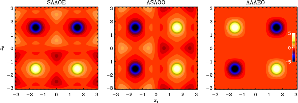
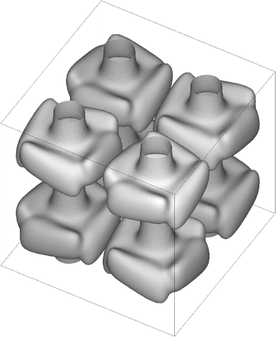
Figure 9: The $x_{3}$-averaged normalised mean fields $\overline{b}_{3}(x_{1},x_{2})/\langle\overline{b}_{3}^{2}\rangle^{1/2}$ for $\eta=0.1$ in the box periodicity of size $(2\pi)^{3}$. The same colour-coding scheme is used in all panels; the data outside the interval $[-5,5]$ is clipped.

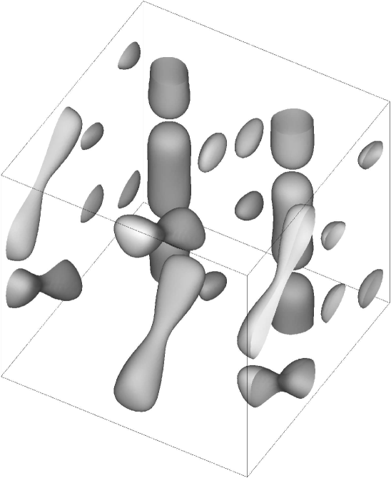
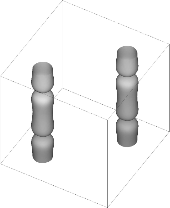
Figure 10: Isosurfaces of the energy for two rms-normalised dominant $2\pi$-periodic modes: SAAOE, $|{\bf b}|^{2}=2$ (left), AAAEO, $|{\bf b}|^{2}=2$ (centre) and AAAEO, $|{\bf b}|^{2}=2/3$ (right).

Figure 11: Isosurfaces of the vertical magnetic field component, $b_{3}=2/3$, for two rms-normalised dominant $2\pi$-periodic modes, ASAOO (left) and AAAEO (right).

Only in 3 subspaces out of 40, growing $2\pi$-periodic magnetic modes have been found (see Table 2). We first inspect suitably averaged fields; as discussed in the next section a particularly revealing average is that over the $x_{3}$ coordinate, the mean field being a function of $x_{1}$ and $x_{2}$. In Fig. 11 we show such mean fields $\overline{b}_{3}(x_{1},x_{2})$; clearly, they do not survive horizontal averaging over the $(x_{1},x_{2})$ plane, because the positive and negative contributions in Fig. 11 cancel. This figure also illustrates some of the symmetries of the invariant subspaces, to which the 3 modes belong. Figures 11 and 11 show isosurfaces of the energy at the level $|{\bf b}|^{2}=2$, and of the vertical magnetic component at the level $b_{3}=2/3$, for two dominant modes, that are not mutually related by any of the symmetries. (The dominant modes in subspaces SAAOE and ASAOO are mapped into each other by the symmetry $\gamma$, and the mode in AAAEO is $\gamma$-symmetric.)

Table 3: Stagnation points of modified Taylor–Green flow (39) for $a=b=1$, and the spectral structure (eigenvalues, $\sigma$, and the proper subspaces) of the Jacobian matrix, $[\partial v^{m}/\partial x_{n}]$, at these points; $j_{i}$ and $j$ are arbitrary integers.

Family	Stagnation point	Proper subspace	Eigenvalue, $\sigma$
		${\bf e}_{1}^{\vphantom{|}}$	$2+(-1)^{j_{1}+j_{2}+j_{3}}(2+3c)$
I	$\pi(j_{1},j_{2},j_{3})$	${\bf e}_{2}$	$2-(-1)^{j_{1}+j_{2}+j_{3}}(2+3c)$
		${\bf e}_{3}$	$-4$
		${\bf e}_{1}$	$-2$
II	$\pi\Big{(}j_{1},j_{2},j_{3}+{1\over 2}\Big{)}$	${\bf e}_{2}$	$-2$
		${\bf e}_{3}$	4
III	$\pi\Big{(}j_{1}+{1\over 2},j_{2}+{1\over 2},j_{3}\Big{)}^{\vphantom{|}}$	$\{{\bf e}_{1},{\bf e}_{2}\}$	$-2\pm{\rm i}\sqrt{c+2}$
		${\bf e}_{3}$	4
		${\bf e}_{1}$	2
IV	$\pi\Big{(}j_{1}+{1\over 2},j_{2}+{1\over 2},j_{3}+{1\over 2}\Big{)}$	${\bf e}_{2}$	2
		${\bf e}_{3}$	$-4$
V	$\pi\Big{(}j_{1}+{1\over 2},j_{2},j_{3}+{1\over 2}\Big{)}^{\vphantom{|}}$	$\sigma{\bf e}_{1}-4(-1)^{j_{1}+j_{2}+j_{3}}(3c-1){\bf e}_{3}$	$1\pm\sqrt{1+4(3c-1)(2-c)}$
		${\bf e}_{2}$	$-2$
VI	$\pi\Big{(}j_{1},j_{2}+{1\over 2},j_{3}+{1\over 2}\Big{)}^{\vphantom{|}}$	$\sigma{\bf e}_{2}+4(-1)^{j_{1}+j_{2}+j_{3}}(3c-1){\bf e}_{3}$	$1\pm\sqrt{1+4(3c-1)(2-c)}$
		${\bf e}_{1}$	$-2$
VII	$(x_{1},j\pi,x_{3})$, where)	${\bf e}_{1}(\sigma-\zeta_{5}(x_{1}))+{\bf e}_{3}\zeta_{6}(x_{1},x_{3})$	$\zeta_{3}(x_{1},x_{3})\pm\sqrt{\zeta_{4}(x_{1},x_{3})}$
	$\sin^{2}x_{1}=\zeta_{2}^{-1}\!\left(\!-\zeta_{1}\pm\sqrt{\zeta_{1}^{2}+4\zeta_{2}}\right)$)	${\bf e}_{2}$	$-2\zeta_{3}(x_{1},x_{3})$
	$\cos x_{3}=(-1)^{j}(3c-1)\sin x_{1}\tan x_{1}$)
VIII	$(j\pi,x_{2},x_{3})$, where)	${\bf e}_{1}$	$-2\zeta_{3}(x_{2},x_{3})$
	$\sin^{2}x_{2}=\zeta_{2}^{-1}\!\left(\!-\zeta_{1}\pm\sqrt{\zeta_{1}^{2}+4\zeta_{2}}\right)$)	${\bf e}_{2}(\sigma-\zeta_{5}(x_{2}))+{\bf e}_{3}\zeta_{6}(x_{2},x_{3})$	$\zeta_{3}(x_{2},x_{3})\pm\sqrt{\zeta_{4}(x_{2},x_{3})}$
	$\cos x_{3}=(-1)^{j}(1-3c)\sin x_{2}\tan x_{2}$)

Here $\zeta_{1}=3c(3c+1)$, $\zeta_{2}=8(3c-1)(2c-1)$, $\zeta_{3}(x,z)=(-1)^{j}\big{(}(3c-1)((3c/2+1)\sin^{2}x-2\sin^{4}x)-\cos 2z\big{)}$,$\zeta_{5}(x)=\big{(}(-1)^{j}(6c-2)-4c+((-1)^{j}(3c-27c^{3})+4-14c+54c^{3})\sin^{2}x\big{)}/(2c-1)$,  $\zeta_{6}(x,z)=4(3c-1)(2-\sin^{2}x)\sin x\sin z$, $\zeta_{4}(x,z)=\big{(}2\sin^{2}z-(8c+(5-19c+3c^{2}+90c^{3})\sin^{2}x)/(1-2c)\big{)}^{2}\!+4(1-3c)(2-\sin^{2}x)\sin^{2}x\sin^{2}z(2+3c-(8-20c)\sin^{2}x)$ for odd $j$ and $\zeta_{4}(x,z)=\big{(}2\cos^{2}z+(-3+3c+9c^{2})\sin^{2}x\big{)}^{2}\!+4(1-3c)(2-\sin^{2}x)\sin^{2}x\sin^{2}z(2+3c-(8-20c)\sin^{2}x)$ for even $j$.

In slow dynamos, magnetic structures can be related to stagnation points of the flow. Eight families of stagnation points of mTG are listed in Table 3; we have checked numerically that no other stagnation points exist in mTG (39), (45). Each of the first four families is a $\gamma$-symmetric set; families V and VI are mapped by $\gamma$ into each other, as well as families VII and VIII. Lines joining stagnation points of family I and parallel to Cartesian axes constitute a heteroclinic network: any such vertical line consists of heteroclinic trajectories connecting adjacent stagnation points of families I and II, and a horizontal line consists of heteroclinic trajectories connecting a pair of adjacent stagnation points of family I. Each plane, parallel to a Cartesian coordinate plane and containing stagnation points of family I, is cut by the aforementioned heteroclinic trajectories into squares of size $\pi$, which are invariant sets for mTG (this stems from the proportionality of $v_{i}$ to $\sin x_{i}$ for each $i$). Vertical and horizontal lines joining stagnation points of family IV constitute another heteroclinic network: they consist of heteroclinic trajectories connecting points of family IV with adjacent stagnation points of families III, V and VI.

The Jacobian matrix of a solenoidal flow generically has either one positive eigenvalue and two eigenvalues with negative real parts, or one negative eigenvalue and two eigenvalues with positive real parts. In the vicinity of a stagnation point of the former kind (having a one-dimensional unstable manifold), magnetic flux ropes usually emerge (Moffatt, 1978; Galloway & Zheligovsky, 1994) that are aligned with the unstable direction. Near a stagnation point of the latter kind (possessing a two-dimensional unstable manifold), magnetic sheets typically emerge (Childress & Soward, 1985) spreading along the unstable manifold. (Formation of these magnetic structures may be prohibited by symmetries.)

We observe such patterns of asymptotic nature, foremost, vertically oriented flux ropes, that are centred at stagnation points of family III (whose one-dimensional unstable manifolds are segments of vertical lines), in the plots of isosurfaces of the magnetic energy at the level $|{\bf b}|^{2}=2$ (Fig. 11, left and central panels) and of the vertical component of magnetic field (Fig. 11) for both modes, shown in the figures, from the symmetry subspaces SAAOE and AAAEO. These “principal” ropes terminate near stagnation points of family IV, whose two-dimensional unstable manifolds are horizontal planes, and which give rise to magnetic field sheets revealed by energy isosurfaces at the low level $|{\bf b}|^{2}=2/3$ (Fig. 11, the right panel). The sheets intermix into vertical flux ropes centred at stagnation points of family II. In the AAAEO mode, adjacent principal flux ropes are oppositely directed (see Fig. 11); consequently, the flux ropes associated with stagnation points of family II are comprised of two pairs of oppositely oriented “flux fibres” (such compound flux ropes were considered by Galloway & Zheligovsky 1994). Since fine structures are accompanied by enhanced dissipation, the compound ropes are weak and not seen in the right panel of Fig. 11 — these relatively high-level isosurfaces only determine the region in space, where the four-fibre flux ropes are located. Compound flux ropes consisting of two oppositely directed fibres centred at stagnation points of families V and VI are present in the AAAEO mode (these individual fibres actually look more like beans in the central panel of Fig. 11: the width of flux ropes is of the order of $R_{m}^{-1/2}$, where $R_{m}$ is the magnetic Reynolds number which is clearly not high for $\eta=0.1$ considered here, and hence the magnetic flux ropes and sheets that we observe are rather “fat”). In the SAAOE mode, flux ropes centred at stagnation points of family VI (but not V) are allowed by the symmetries defining the subspace; these flux ropes do not have a fibre structure (in the left panel of Fig. 11 they are cut into halves by the faces of the shown cube of periodicity) and their energy content is even higher than that of the principal ropes.

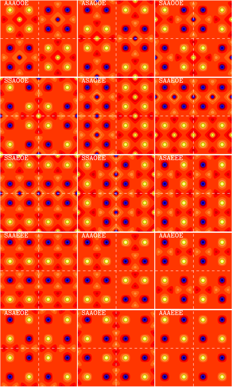
Figure 12: The $x_{3}$-averaged normalised mean field $\overline{b}_{3}(x_{1},x_{2})/\langle\overline{b}_{3}^{2}\rangle^{1/2}$ for $\eta=0.1$ in a domain of size $(4\pi)^{3}$. The white dashed lines mark subdomains of size $(2\pi)^{2}$. Same colour-coding scheme as in Fig. 11.

       

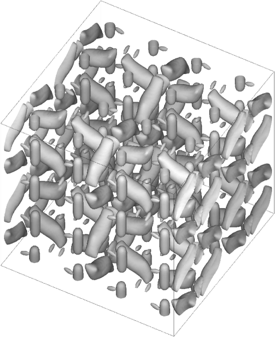
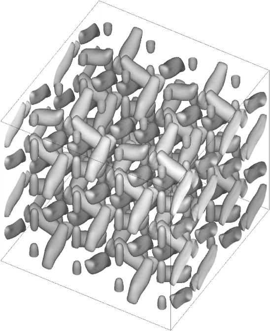
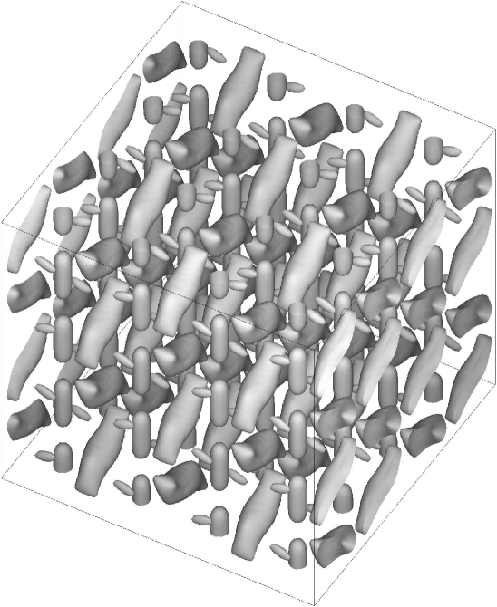
ASAOOE                                                                           ASAOEE                                                                           ASAEEE

       

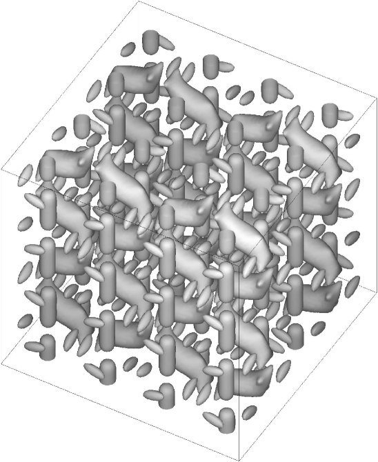
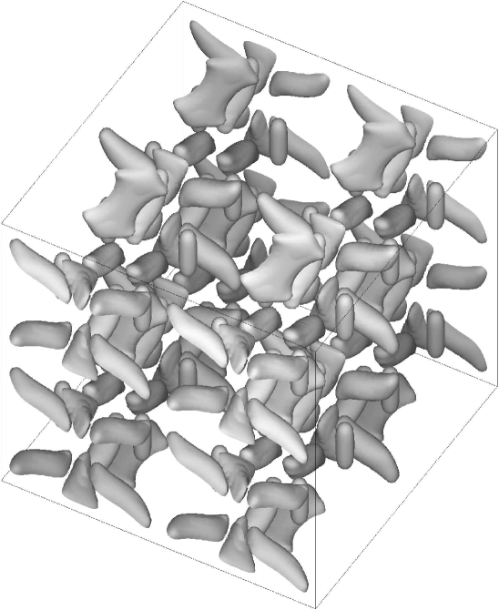
AAAOEE                                                                           AAAEEE                                                                           SASOOO

Figure 13: Isosurfaces of the energy for six rms-normalised isotypic dominant $4\pi$-periodic modes at the level $|{\bf b}|^{2}=2$.

       

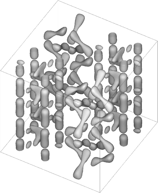
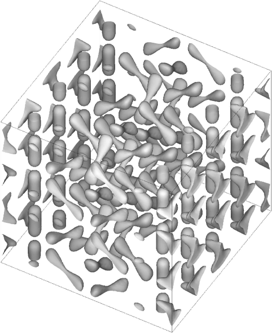
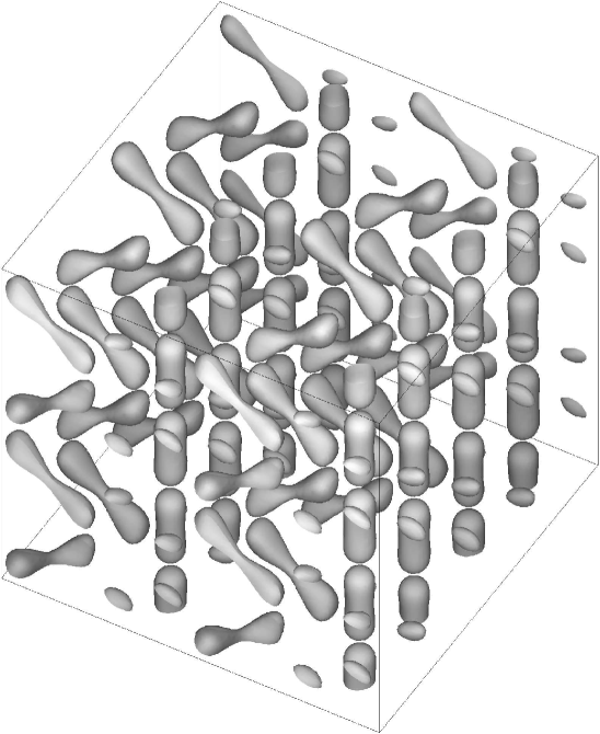
AAAOOE                                                                           SSAEOE                                                                           SAAEEE

       

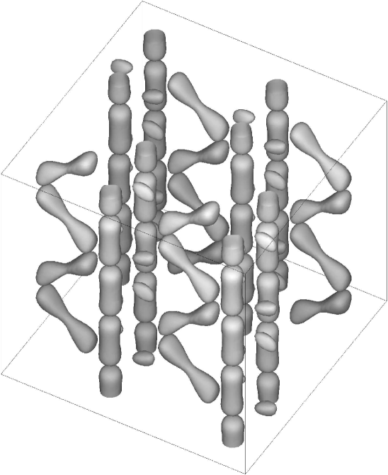
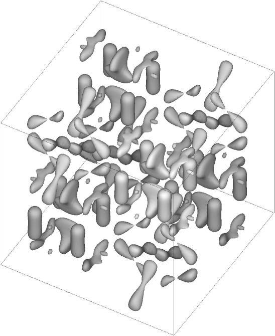
AAAOEE                                                                           AAAEEE                                                                           AASOOO

Figure 14: Isosurfaces of the vertical magnetic component for six rms-normalised isotypic dominant $4\pi$-periodic modes at the level $b_{3}=2/3$.

All $4\pi$-periodic magnetic modes, growing for $\eta=0.1$, are also listed in Table 2. Such modes can be symmetric or antisymmetric in each Cartesian variable $x_{i}$; this is coded by the first 3 characters in the labels (letters $\tt S$ and $\tt A$, respectively) of invariant subspaces, like in the case of $2\pi$-periodic modes. The trailing 3 characters of the 6-character labels have now a new meaning: for any fixed $i$, the wave numbers $k_{i}$ in all Fourier harmonics ${\rm e}^{{\rm i}{\bf k\cdot x}/2}$ comprising a $4\pi$-periodic mode have the same parity, which is indicated by letters $\tt E$ or $\tt O$ (even and odd values, respectively) in position $i+3$. We have considered neither the more subtle parity symmetries, nor the $\gamma$-symmetry. Since the 6 aforementioned symmetries are independent, they split the domain of the magnetic induction operator into 64 invariant subspaces. We have computed dominant magnetic modes in each of them using $128^{3}$ Fourier harmonics (before dealiasing), which effectively provide the same spatial resolution as $64^{3}$ harmonics in computations of the $2\pi$-periodic modes.

For the dominant growing $4\pi$-periodic magnetic modes, we show the same plots as for the $2\pi$-periodic ones: the mean fields $\overline{b}_{3}(x_{1},x_{2})$ averaged over $x_{3}$ for 15 dominant $4\pi$-periodic modes (Fig. 12), and isosurfaces of the energy $|{\bf b}|^{2}=2$ and of the component $b_{3}=2/3$ for six of them, that are not mutually related by any symmetry (Figs. 13 and 14). Clearly, the averages over the $(x_{1},x_{2})$ plane of the vertical component $b_{3}$ for all dominant modes shown in Fig. 12 are zero, as this was the case for the $2\pi$-periodic modes. (For the 8 growing modes comprising the last group in Table 2, $\overline{b}_{3}=0$, because they involve only odd wave numbers $k_{3}$.) The most prominent features in Fig. 12 are the averages of the vertically oriented flux ropes centred at stagnation points of family III; all other flux ropes cancel out upon averaging over $x_{3}$ either mostly or completely. It is natural that these mean flux ropes of a similar genesis have a similar shape in all panels in Fig. 12 and, for instance, have close extremum values, the maxima ranging from 5.72 for dominant modes from the second group of $4\pi$-periodic modes in Table 2 (including subspace ASAOEE) to 6.62 in the fifth group (subspace AAAEEE). (The maxima are computed for the normalised averages $\overline{b}_{3}(x_{1},x_{2})/\langle\overline{b}_{3}^{2}\rangle^{1/2}$.) It turns out that the dominant $4\pi$-periodic modes in subspaces ASAEEE, SAAEEE and AAAEEE are just the tiling of the cube of periodicity of size $4\pi$ by 8 cubes of periodicity of size $2\pi$ with $2\pi$-periodic modes in subspaces ASAOO, SAAOE and AAAEO, respectively (note that the growth rates of the respective $4\pi$- and $2\pi$-periodic modes coincide). In fact, each group of $4\pi$-periodic modes that have the same growth rate (see Table 2) are related by symmetries. (For instance, the eight slowest-growing modes constituting the last group in Table 2 are mutually related by combinations of shifts by $2\pi$ along the Cartesian axes.)

5.4 DNS and TFM results for eddy diffusivity in mTG

As noted above, horizontal averaging over the $(x_{1},x_{2})$ plane cannot be applied to describe a growing mean field generated by mTG. Indeed, averaging the solenoidality condition for $\bf b$ we find that $\overline{b}_{3}$ is spatially uniform at all times; then the spatial average of the third component of (1) shows that it is also time-independent. Since $\overline{b}_{3}$ cannot grow or decay, such an average is unsuitable for studying the negative eddy diffusivity dynamo for mTG (for which we are advised by MST that $\overline{b}_{3}\neq 0$, see (46)). By contrast, planar averages can describe growing solutions in the supercritical case, if one averages along $x_{3}$ and a diagonal direction, or uses any of the two other planar averages, over $(x_{1},x_{3})$ or $(x_{2},x_{3})$. Note that, for a flow with a large group of symmetries, any planar averaging may yield, due to cancellation, identically zero averages for modes in certain symmetry subspaces. For instance, for mTG, no cancellation occurs for the $(x_{1},x_{3})$ or $(x_{2},x_{3})$ averagings for the second and third groups of $4\pi$-periodic modes in Table 2, and for diagonal ones for the first and fifth groups. Thus, the average over $(x_{1},x_{3})$ or $(x_{2},x_{3})$ is adequate in 6 subspaces; the diagonal average in 5 subspaces, including the dominant one; and none in the remaining 12 subspaces containing growing modes. None of the easily implementable planar averagings is universally applicable.

We now consider averaging over the $(x_{2},x_{3})$ plane. The evolution of the auxiliary fluctuating field is now controlled by the operator $\bm{\mathfrak{P}}\L\bm{\mathfrak{P}}$, where $\bm{\mathfrak{P}}$ is the projection that deletes the mean field, but preserves the volume average, and $\L$ is the operator of magnetic induction. The dominant modes of the new operator belong to a symmetry subspace, different from those, where the dominant modes of $\L$ acting alone reside (see in the left panel of Fig. 15 the mean saturated magnetic field produced by DNS with the use of the Pencil Code). Despite the additional projections, the main visible magnetic structures are still the vertical flux ropes centred at the family III stagnation points of mTG. The right panel of Fig. 15 shows the mean field (which is now a function of $x_{1}$). It has positive and negative extrema at $x_{1}=\mp\pi/2$. Our computations also reveal that the two possible mean fields, $\overline{b}_{3}(x_{1})$ and $\overline{b}_{3}(x_{2})$, have the same shape. Again, the mean field is anharmonic and therefore the eddy diffusivity cannot be spatially constant.

Owing to the anharmonic nature of the resulting mean fields, we must consider test fields involving many Fourier harmonics. Let us begin with the most important contribution from $k_{1}=1$. We use again the Pencil Code, where TFM is readily implemented. In all the cases presented below we have used $72^{3}$ mesh points. In Fig. 17 we show the results for $\eta_{22}(x_{1})$ and $\eta_{33}(x_{1})$ for $\eta=0.1$ and $k_{1}=1$. Note that both $\eta_{11}$ and $\eta_{33}$ show strong spatial variations. However, while $\eta_{33}$ is always positive, $\eta_{11}$ has extended regions where it is negative, giving rise to growth of $\overline{b}_{3}(x_{1})$.

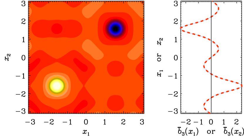
Figure 15: The $x_{3}$-averaged rms-normalised mean field $\overline{b}_{3}(x_{1},x_{2})/\langle\overline{b}_{3}^{2}\rangle^{1/2}$ from DNS for $\eta=0.1$ in a domain of size $(2\pi)^{3}$ (left panel) and the planar average $\overline{b}_{3}(x_{1})$ (obtained by averaging over $x_{2}$ and $x_{3}$, black line), and $\overline{b}_{3}(x_{2})$ (averaging over $x_{1}$ and $x_{3}$, red dashed line overplotted). Same colour-coding scheme as in Fig. 12.

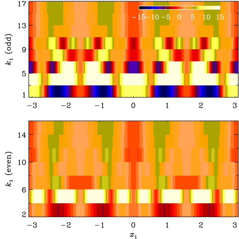
Figure 16: $\eta_{22}(x_{1})$ and $\eta_{33}(x_{1})$ for $\eta=0.1$ and $k_{1}=1$. $\eta_{22}(x_{1})$ has a negative average, indicated by the dotted line.

Figure 17: $\eta_{22}(x_{1},k_{1},0)k_{1}^{2}$ for $\eta=0.1$ shown colour-coded separately for odd (upper panel) and even (lower panel) values of $k_{1}$. Same colour-coding scheme on both panels.

In principle, negative diffusivities can be used in a numerical mean-field simulation. However, one would then need to include contributions from larger wave numbers $k_{1}$ (or $\epsilon$), where $\eta_{22}$ eventually becomes positive for large wave numbers. This was demonstrated in Devlen et al. (2013), where the turbulent diffusivity kernel was spatially constant, and so the relevant eigenvalue problem became

$$\Lambda\hat{A}_{2}=-(\eta+\eta_{22}(k_{1},{\rm i}\Lambda))\,k_{1}^{2}\hat{A}_{2}$$

(cf. (16)). Here, $\hat{A}_{2}$ is the Fourier amplitude and, for consistency (cf. (4)–(5)), the eddy correction $\eta_{22}$ should be calculated for $\omega={\rm i}\Lambda$, which is in general complex. In the present case, we only find non-oscillatory growth, so $\Lambda$ is real and therefore the frequency $\omega$, for which $\eta_{22}$ is needed, is purely imaginary. Since the dependence of $\eta_{22}$ on $\omega$ is in general nonlinear, one has a nonlinear eigenvalue problem that can be solved iteratively. Even in the simplest cases considered by Hubbard & Brandenburg (2009), $\eta_{22}$ is proportional to $1/(1-{\rm i}\omega\tau)$, where $\tau$ is the memory time. To understand this proportionality for large $|\omega|$, we note that for test fields (7) we find from (2)

$${\bf b^{\prime}}={\rm i}\omega^{-1}\left(\L_{\varepsilon\bf q}{\bf e}_{n}+{\rm O}(|\omega|^{-1})\right),$$

where $\varepsilon{\bf q}={\bf k}$ in the definition (48) of the operator $\L_{\varepsilon\bf q}$. An illustrative example of the iterative procedure was given by Rheinhardt et al. (2014) for a more complicated case where $\omega={\rm i}\Lambda$ was complex. We can encounter a neutral dynamo such that Re$\Lambda=0$ (this usually occurs for a specific value of $k_{1}$) by increasing $k_{1}$, i.e., decreasing the domain; see Figs. 1 and 2 of Rheinhardt et al. (2014) for a related problem.

In the present case, because $\eta_{22}(x_{1})$ is nonuniform, we have to allow for all possible wave numbers of the resulting mean field and compute the response for each wave number. This is just opposite to the usual mean-field dynamo problem and the MST approach where one computes the dynamo effects in the limit ${\bf k}\to 0$. The relevant eigenvalue problem for our domain of size $2\pi$ now becomes

$$\Lambda A_{2}(x_{1})=-\sum_{k_{1}=1}^{\infty} (\eta+\eta_{22}(x_{1},k_{1},{\rm i}\Lambda))k_{1}^{2}$$

$$\times\int_{-\pi}^{\pi}{\rm e}^{{\rm i}k_{1}(x_{1}-\xi_{1})}A(\xi_{1})\,{\rm d}\xi_{1}.$$ (61)

In Fig. 17 we have already plotted $\eta_{22}(x_{1},1,0)$, but we now need $\eta_{22}(x_{1},k_{1},{\rm i}\Lambda)$ for all integer values of $k_{1}$ and a suitable value of $\omega$.

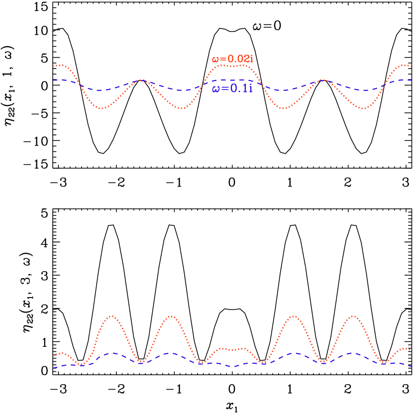
Figure 18: Compensated kernel $\eta_{22}(x_{1},1,\omega)$ (upper panel) and $\eta_{22}(x_{1},3,\omega)$ (lower panel) for $\omega=0$ (black solid line), $0.02{\rm i}$ (red dotted line), and $0.1{\rm i}$ (blue dashed line) using $\eta=0.1$.

Figure 19: Dependence of $\eta+\langle\eta_{22}\rangle$ on $k_{1}$, obtained with TFM by computing a steady solution to (59) (solid line), versus the results of the Pencil Code (filled symbols). For comparison, $\eta+\langle\eta_{33}\rangle$ is shown (hollow symbols). Here, $\eta=0.1$, $\omega=0$.

Note that for our domain of size $2\pi$ the permissible wave numbers $k_{1}$ are integers. Furthermore, looking at the right panel of Fig. 15, we see that the eigenfunction is odd about $x_{1}=0$. This means that only odd values of $k_{1}$ contribute to the solution. In agreement with our earlier experience, the amplitudes of the turbulent transport coefficients fall off quadratically with increasing wave number (see, e.g., Brandenburg et al., 2008b). We therefore expect that the compensated expression $\eta_{22}(x_{1},k_{1},{\rm i}\Lambda)k_{1}^{2}$ should be independent of $k_{1}$ for large values. This is indeed the case, as can be seen from Fig. 17, where we plot $\eta_{22}(x_{1},k_{1},0)k_{1}^{2}$ separately for odd and even values of $k_{1}$.

We should point out that these results are sensitive to the values of $\eta$ and $\omega$, as will be demonstrated next. First, in Fig. 19 we plot $\eta_{22}(x_{1},k_{1},{\rm i}\Lambda)$ for $\omega=0$, $0.02{\rm i}$ and $0.1{\rm i}$, and for $k_{1}=1$ and 3. While the shapes of the different curves remain similar, there is a significant reduction in the amplitude as $\omega$ increases. Thus, it is in general impossible to omit the memory effect. This agrees with earlier results for certain steady flows (Rädler et al., 2011; Rheinhardt et al., 2014), although it is not a typical feature of turbulent flows (Hubbard & Brandenburg, 2009). Second, we give in Table 5 the volume-averaged values $\langle\eta_{22}\rangle$ and $\langle\eta_{33}\rangle$ for $\omega=0$ and different values of $\eta$. It turns out that $\eta+\langle\eta_{22}\rangle=-0.017$ for $\eta=0.115$, tentatively suggesting that this case is weakly supercritical, while for $\eta=0.120$ we have $\eta+\langle\eta_{22}\rangle=+0.053$, which would be clearly subcritical. These values are close to those obtained from DNS, which show that the critical value of $\eta$ for the onset of generation of magnetic field with the periodicities of the flow is around 0.1105 (see also Table 1). For more precise statements we would need to consider numerical solutions to (61).

Table 4: $\langle\eta_{22}\rangle$ and $\langle\eta_{33}\rangle$ computed for $\omega=0$ and various $\eta$.

$\eta$	$\langle\eta_{22}\rangle$	$\langle\eta_{33}\rangle$
0.100	$-1.858$	0.230
0.110	$-0.245$	0.239
0.115	$-0.117$	0.242
0.120	$-0.047$	0.244

Table 5: Comparison between $\eta+\langle\eta_{22}\rangle$, obtained with TFM by computing a steady solution to (59) (first column, marked by an asterisk), and $\langle\eta_{22}\rangle$ as well as $\langle\eta_{33}\rangle$ obtained with the Pencil Code for $\eta=0.1$, $\omega=0$ and various $k_{1}$.

$k_{1}$	$\eta+\langle\eta_{22}\rangle^{*}$	$\langle\eta_{22}\rangle$	$\langle\eta_{33}\rangle$
2.5	$+1.05656$	$+0.9559$	0.1843
2.0	$+0.20545$	$+0.1055$	0.1843
1.5	$-0.34576$	$-0.4460$	0.1808
1.0	$-1.75831$	$-1.858$	0.2304
0.5	$-2.11246$	$-2.213$	0.3051
0.25	$-2.02750$	$-2.127$	0.3210

The $k_{1}$-dependence of eddy diffusivity $\eta+\langle\eta_{22}\rangle$ is shown in Fig. 19 and numerical values are given in Table 5 for $\eta=0.1$ and $\omega=0$. Here we compare the results from TFM obtained with the Pencil Code with those obtained by cancelling the exponential factor and determining steady solutions to (59); the latter were computed by the code by Fokkema (1995), employing the biconjugate gradients stabilised method BiCGstab($\ell$) for $\ell=6$ (see Sleijpen & Fokkema 1993; Sleijpen & van der Vorst 1995, 1996). We also show $\eta+\langle\eta_{33}\rangle$ which is always positive. Note that $\eta+\langle\eta_{22}\rangle$ becomes zero at $k_{1}\approx 1.8$. Thus in our domain of size $2\pi$, where $k_{1}=1$ is the smallest wave number, the volume-averaged eddy diffusivity is clearly negative.

6 Concluding remarks

In mean-field electrodynamics, various analytical and numerical approaches are used to express the mean electromotive force, originally defined in terms of small-scale fluctuations of flow velocity and magnetic field, as functions of the large-scale mean flow and magnetic field. Assessing the range of validity and clarifying conflicts in application of these approaches is crucial in view of many applications, e.g., in laboratory experiments for dynamo generation or in astrophysics. For instance, a comparison of the traditional MFE approach with those based on $\tau$-approximations of turbulence theory was carried out by Rädler & Rheinhardt (2007). Here, we have compared two different methods for estimation of the mean e.m.f.: MST, which explicitly considers steady or time-periodic laminar flows, and TFM, which is not affected by such a restriction. For instance, Cabanes et al. (2014) recently observed in a rotating liquid sodium experiment “Derviche Tourneur Sodium” a reduction of the effective magnetic diffusivity in some regions of the flow, probably caused by the turbulence; it is thus important to assess, under which conditions the methods investigated here can be used to study this kind of problems.

We have demonstrated that, in the two-scale setup, magnetic eddy diffusivities predicted by MST in three-dimensional small-scale steady flows are reproduced by TFM, provided volume averaging is used. It can be similarly shown that the same result holds true for time-periodic flows — in this case the averaging procedure must also involve time averaging over the temporal period. If other types of averaging (planar or over just one Cartesian variable) are applied, one can, in general, only expect a qualitative agreement between the results. One must also be aware of the following caveat: Because of the asymptotic character of the MST results, achieving agreement with TFM eddy diffusivities requires small scale ratios $\varepsilon$ and thus high spatial resolution to be used when solving the TFM test problems (2). This can be seen as a drawback of TFM in comparison with MST.

Results coinciding with those of MST can also be obtained by a modified TFM algorithm that proceeds by setting a test field as initial condition and solving the standard magnetic induction equation (60) without separating the field into mean and fluctuating parts before the saturated regime for the magnetic field sets in, and then computing the e.m.f. due to the fluctuating flow and magnetic field as in the canonical TFM. Reliance of TFM on the integral (3) approximation of the e.m.f., resulting in the ansatz (4) (or (57)) for the Fourier transforms, then proves crucial. This feature of TFM implies that, in the multiscale limit $\varepsilon\to 0$, the choice of the spatial variables for averaging becomes insignificant, because the use of the Fourier transform over the remaining variables effectively converts all the averages into averages over all the three spatial variables (see (55) and (58)). This observation does not hold for the conventional version of MFE, where the e.m.f. is approximated by local differential operators. Nevertheless, the MST $\alpha$-effect tensor in small-scale flows can be computed by TFM with the use of constant test fields and full spatial averaging.

We have numerically confirmed the findings of Lanotte et al. (1999) that the modified Taylor–Green flow possesses, in certain ranges of parameter values, negative eddy diffusivities, and have shown that the same holds for the G.O. Roberts flow IV. This is in contrast with Devlen et al. (2013), who did not find negative eddy diffusivity for the former flow. Why did Lanotte et al. (1999) and Devlen et al. (2013) arrive to different conclusions for this flow? We have seen that the results of MST and TFM do not agree qualitatively unless TFM applies volume averaging (R-IV depending on two spatial variables is a special case), but a number of less important reasons make the picture even more complicated: ($i$) We have now obtained negative eddy diffusivities in mTG by TFM, but we have been forced to employ a planar averaging different from the one used by Devlen et al. (2013). ($ii$) Eddy diffusivities affecting the evolution of large-scale perturbations of distinct short-scale magnetic modes do not coincide. While Lanotte et al. (1999) considered eddy diffusivity for the neutral short-scale modes, Devlen et al. (2013) aimed at evaluating it for the dominant short-scale modes, which for $\eta=0.02$ is a distinct branch; hence, there are no reasons to expect their results on eddy diffusivity to be interrelated. ($iii$) Furthermore, at large scale separations (i.e., small $\varepsilon$) the eddy diffusivity for the dominant branch for $\eta=0.02$ is negative (see Fig. 6); in this case, TFM still can be used to evaluate the eddy diffusivity, but special precautions must be taken in its implementation: TFM requires solving test problems (2), which are likely to inherit the instability of the unperturbed magnetic induction equation (60) and have exponentially growing modes. In the course of numerical integration, the growing modes will then set in due to the influence of round-off errors and progressively wipe out the contribution of the inhomogeneity in (2), which we intend to determine. A feasible strategy is to compute directly a time-independent solution to (2) regarded as a system of linear equations (after a suitable discretisation of the problem in space).

Investigation of eddy diffusivity is supposed to yield the effective diffusivity which can be employed, e.g., to study nonlinear large-scale MHD regimes. Our results demonstrate that this may be a non-realistic goal. Magnetic field in a nonlinear MHD regime can be decomposed into a linear combination of eigenmodes of the magnetic induction operator, where the coefficients are time-dependent. We have presented growth rates in branches of dominant large-scale magnetic eigenmodes generated by mTG in four symmetry subspaces. The parabolic shape of their plots as functions of the scale ratio $\varepsilon$ near $\varepsilon=0$ or 1 confirms that the phenomenon of magnetic eddy diffusivity is observed for sufficiently large scale separations in all branches. However, Fig. 6 also shows that the curvature of the parabola varies significantly for different branches of modes. Hence, for a given molecular diffusivity, no universal eddy diffusivity tensor can be assigned to a given generating flow, because the action of eddy diffusivity significantly depends on the spectral composition of the multiscale magnetic field itself, on which such an integral diffusivity acts. We are thus forced to conclude that a unified description of “average” magnetic eddy diffusivity would only be possible in the case of a turbulent MHD regime with a well-defined statistics of the spectral composition of magnetic field — for instance, when a chaotic attractor of an MHD dynamical system is considered. (As a side remark, we note that the same holds true for the $\alpha$-effect tensor: for large-scale permutations of different small-scale magnetic modes generated by small-scale non-symmetric flows, generically different tensors are obtained, and hence the integral $\alpha$-effect tensor depends on the spectral composition of the magnetic field.) From this prospective, the TFM approach seems advantageous, since it demands to separately quantify the influence of each Fourier harmonics in the mean magnetic field by nominating it as a test field and computing the fluctuating field that it induces and the respective output e.m.f., and afterwards to sum up such contributions of each individual harmonics into the integral output.

Let us note some open questions, beginning with the most important one.

1. TFM follows MFE in relying on approximations such as (3) (e.g., the precise kernels in (3) are not translation-invariant). It is essential, that nevertheless in some limits (the most important of which is the limit of small magnetic Reynolds numbers) MFE yields results that are exact, i.e., TFM and MFE agree exactly and in all details with DNS (see the review by Brandenburg et al., 2010). Given that ($i$) we know that MST is a precise corollary of the basic equations, and ($ii$) we have observed that MST can quantitatively disagree with TFM, we need to understand the mathematical reasons for the aforementioned agreement in the respective limits. The availability of precise mathematical demonstrations may help to determine the conditions, under which TFM can be used reliably.

2. As we have mentioned in the Introduction, the generated large-scale structures are described by amplitudes (depending exclusively on slow variables) of the small-scale neutral (magnetic or MHD stability) modes that constitute the leading term in the expansion of perturbation in the scale ratio. In two-scale systems (such as the ones considered here), the temporal evolution of the amplitudes is governed by equations (mean-field or otherwise), where the $\alpha$-effect operator is never present together with the eddy diffusivity operator: since the orders of these differential operators are different, they emerge at different orders of the scale ratio. (A joint action of molecular diffusivity and the $\alpha$-effect is encountered in flows with an internal spatial scale, see Chaps. 10 and 11 in Zheligovsky 2011.) Do the two operators appear simultaneously in amplitude equations in a truly multiple-scale setup? In other words, can in such a setup the mean e.m.f. be a sum of the $\alpha$- and $\eta$-terms, as this was assumed in the early variants of MFE?

3. Expressing entries of the magnetic eddy diffusivity correction tensor in terms of solutions to auxiliary problems for the adjoint operator has proved useful not only for reducing the amount of computations, but also in analytical work, for establishing relations (29) between the tensors for opposite flows, and for identifying zero entries of the tensor for translation-invariant flow (see Section 3). In these calculations we have relied on the similarity of the magnetic induction operator and the adjoint operator for the reverse flow. Do solutions to the auxiliary problem for the adjoint operator have a physical interpretation?

4. Finally, the following technical question is of certain interest: Eq. (2) governing the evolution of the fluctuating magnetic field involves the operator $\bm{\mathfrak{P}}\L\bm{\mathfrak{P}}$, where $\bm{\mathfrak{P}}$ projects out the mean field and $\L$ is the usual operator of magnetic induction. Suppose that there is no small-scale dynamo action, i.e., all eigenvalues of $\L$ have non-positive real parts, and an averaging other than volume averaging is employed. Is it then possible, for some flows and some test fields, to have growing fluctuating solutions, i.e., can the operator $\bm{\mathfrak{P}}\L\bm{\mathfrak{P}}$ have an eigenvalue with a positive real part?

References

- Blackman & Field (2002) Blackman E.G., Field G.B. New dynamical mean-field dynamo theory and closure approach. Phys. Rev. Lett. 89, 2002, 265007.
- Brandenburg et al. (2010) Brandenburg A., Chatterjee P., Del Sordo F., Hubbard A., Käpylä P.J., Rheinhardt M. Turbulent transport in hydromagnetic flows. Phys. Scr. T142, 2010, 014028.
- Brandenburg et al. (2008a) Brandenburg A., Rädler K.-H., Rheinhardt M., Käpylä P.J. Magnetic diffusivity tensor and dynamo effects in rotating and shearing turbulence. Astrophys. J. 676, 2008a, 740–751.
- Brandenburg et al. (2008b) Brandenburg A., Rädler K.-H., Schrinner M. Scale dependence of alpha effect and turbulent diffusivity. Astron. Astrophys. 482, 2008b, 739–746.
- Cabanes et al. (2014) Cabanes S., Schaeffer N., Nataf H.-C. Turbulence reduces magnetic diffusivity in a liquid sodium experiment. Phys. Rev. Lett. 113, 2014, 184501-1–5.
- Cattaneo & Hughes (2006) Cattaneo F., Hughes D.W. Dynamo action in a rotating convective layer. J. Fluid Mech. 553, 2006, 401–418.
- Cattaneo & Hughes (2008) Cattaneo F., Hughes D.W. The alpha-effect in rotating convection: size matters. J. Fluid Mech. 594, 2008, 445–461.
- Chertovskih et al. (2010) Chertovskih R., Gama S.M.A., Podvigina O., Zheligovsky V. Dependence of magnetic field generation by thermal convection on the rotation rate: a case study. Physica D, 239, 2010, 1188–1209. http://arxiv.org/abs/0908.1891 .
- Chertovskih & Zheligovsky (2015) Chertovskih R., Zheligovsky V. Large-scale weakly nonlinear perturbations of convective magnetic dynamos in a rotating layer. Physica D, submitted, 2015.
- Childress & Soward (1985) Childress S., Soward A.M. On the rapid generation of magnetic field. Proc. NATO Advanced research workshop on Chaos in Astrophysics (NATO ASI Series. Ser. C, vol. 161). Eds. Buchler J.R., Perdang J.M., Spiegel E.A. D. Reidel Publ. Co., Dordrecht, Holland, 1985, 233–244.
- Devlen et al. (2013) Devlen E., Brandenburg A., Mitra D. A mean field dynamo from negative eddy diffusivity. Mon. Not. R. Astron. Soc. 432, 2013, 1651–1657.
- Dubrulle et al. (2007) Dubrulle B., Blaineau P., Mafra Lopes O., Daviaud F., Laval J.-P., Dolganov R. Bifurcations and dynamo action in a Taylor–Green flow. New J. Physics, 9, 2007, 308, 1–38. http://m.iopscience.iop.org/1367-2630/9/8/308 .
- Dubrulle & Frisch (1991) Dubrulle B., Frisch U. Eddy viscosity of parity-invariant flow. Phys. Rev. A, 43, 1991, 5355–5364.
- Fokkema (1995) Fokkema D.R. Subroutine BISTBL. 1995. http://www.staff.science.uu.nl/~vorst102/software.html .
- Frisch et al. (1987) Frisch U., She Z.S., Sulem P.L. Large-scale flow driven by the anisotropic kinetic alpha effect. Physica D, 28, 1987, 382–392.
- Galloway & Zheligovsky (1994) Galloway D.J., Zheligovsky V.A. On a class of non-axisymmetric flux rope solutions to the electromagnetic induction equation. Geophys. Astrophys. Fluid Dyn. 76, 1994, 253–264.
- Hubbard & Brandenburg (2009) Hubbard A., Brandenburg, A. Memory effects in turbulent transport. Astrophys. J., 706, 2009, 712–726.
- Kato (1966) Kato T. Perturbation theory for linear operators. Springer-Verlag, Berlin, 1966.
- Kraichnan (1971) Kraichnan R.H. An almost-Markovian Galilean-invariant turbulence model. J. Fluid Mech. 47, 1971, 513–524.
- Krause & Rädler (1980) Krause F., Rädler K.-H. Mean-field magnetohydrodynamics and dynamo theory. Pergamon Press, Oxford, 1980.
- Lanotte et al. (1999) Lanotte A., Noullez A., Vergassola M., Wirth A. Large-scale dynamo by negative magnetic eddy diffusivities. Geophys. Astrophys. Fluid Dyn. 91, 1999, 131–146.
- Moffatt (1978) Moffatt H.K. Magnetic field generation in electrically conducting fluids. Cambridge Univ. Press, 1978.
- Rädler (2007) Rädler K.-H. Mean-field dynamo theory: early ideas and today’s problems. In Magnetohydrodynamics. Historical evolution and trends. Eds. S. Molokov, R. Moreau, K. Moffatt. Fluid mechanics and its applications, vol. 80. Springer, 2007, 55–72.
- Rädler et al. (2011) Rädler K.-H., Brandenburg A., Del Sordo F., Rheinhardt M. Mean-field diffusivities in passive scalar and magnetic transport in irrotational flows. Phys. Rev. E, 84, 2011, 046321.
- Rädler & Rheinhardt (2007) Rädler K.-H., Rheinhardt M. Mean-field electrodynamics: critical analysis of various analytical approaches to the mean electromotive force. Geophys. Astrophys. Fluid Dyn. 101, 2007, 117–154.
- Rheinhardt & Brandenburg (2012) Rheinhardt M., Brandenburg A. Modeling spatio-temporal nonlocality in mean-field dynamos. Astron. Nachr. 333, 2012, 71–77.
- Rheinhardt et al. (2014) Rheinhardt M., Devlen E., Rädler K.-H., Brandenburg A. Mean-field dynamo action from delayed transport. Mon. Not. R. Astron. Soc., 441, 2014, 116–126.
- G.O. Roberts (1972) Roberts G.O. Dynamo action of fluid motions with two-dimensional periodicity. Phil. Trans. Roy. Soc. Lond. A271, 1972, 411–454.
- Schrinner et al. (2005) Schrinner M., Rädler K.-H., Schmitt D., Rheinhardt M., Christensen U.R. Mean-field view on rotating magnetoconvection and a geodynamo model. Astron. Nachr. 326, 2005, 245–249.
- Schrinner et al. (2007) Schrinner M., Rädler K.-H., Schmitt D., Rheinhardt M., Christensen U.R. Mean-field concept and direct numerical simulations of rotating magnetoconvection and the geodynamo. Geophys. Astrophys. Fluid Dyn. 101, 2007, 81–116.
- Sleijpen & Fokkema (1993) Sleijpen G.L.G., Fokkema D.R. BiCGstab() for linear equations involving unsymmetric matrices with complex spectrum. ETNA, 1, 1993, 11–32.
- Sleijpen & van der Vorst (1995) Sleijpen G.L.G., van der Vorst H.A. Maintaining convergence properties of BiCGstab methods in finite precision arithmetic. Numerical Algorithms, 10, 1995, 203–223.
- Sleijpen & van der Vorst (1996) Sleijpen G.L.G., van der Vorst H.A. Reliable updated residuals in hybrid BiCG methods. Computing, 56, 1996, 141–163.
- Steenbeck, Krause & Rädler (1966) Steenbeck M., Krause F., Rädler K.-H. Berechnung der mittleren Lorentz-Feldstärke für ein elektrisch leitendes Medium in turbulenter, durch Coriolis–Kräfte beeinfluißter Bewegung. Z. Naturforsch. 21a, 1966, 369–376. Engl. transl.: A calculation of the mean electromotive force in an electrically conducting fluid in turbulent motion, under the influence of Coriolis forces. In Roberts P.H., Stix M. The turbulent dynamo: A translation of a series of papers by F. Krause, K.-H. Rädler, and M. Steenbeck. Tech. Note NCAR-TN/IA-60, Boulder, Colorado, 1971, 29–47. http://nldr.library.ucar.edu/repository/assets/technotes/TECH-NOTE-000-000-000-045.pdf .
- Stone & Goldbart (2009) Stone M., Goldbart P. Mathematics for physics. A guided tour for graduate students. Cambridge Univ. Press, 2009.
- Sulem et al. (1975) Sulem P.L., Lesieur M., Frisch U. Le Test-Field Model interprété comme une méthode de fermeture des équations de la turbulence. Ann. Géophys. 31, 1975, 487–495.
- Tilgner (2004) Tilgner A. Small scale kinematic dynamos: beyond the -effect. Geophys. Astrophys. Fluid Dyn. 98, 2004, 225–234.
- Vishik (1987) Vishik M.M. Periodic dynamo. In Mathematical methods in seismology and geodynamics (Computational seismology, 19). Eds. Keilis-Borok V.I., Levshin A.L. Nauka, Moscow, 1986, 186–215. Engl. transl.: Computational seismology, 19. Allerton Press, New York, 1987, 176–209.
- Zheligovsky (1993) Zheligovsky V. Numerical solution of the kinematic dynamo problem for Beltrami flows in a sphere. J. Scientific Computing, 8, 1993, 41-68.
- Zheligovsky (2003) Zheligovsky V.A. On the linear stability of steady space-periodic magnetohydrodynamic systems to large-scale perturbations. Physics of the Earth № 5, 2003, 65–74. Engl. transl.: Zheligovsky V.A. On the linear stability of spatially periodic steady magnetohydrodynamic systems with respect to long-period perturbations. Izvestiya, Physics of the Solid Earth, 39, 2003, 409–418.
- Zheligovsky (2011) Zheligovsky V.A. Large-scale perturbations of magnetohydrodynamic regimes: linear and weakly nonlinear stability theory. Lecture notes in physics, vol. 829, Springer-Verlag, Heidelberg, 2011.
- Zheligovsky et al. (2001) Zheligovsky V.A., Podvigina O.M., Frisch U. Dynamo effect in parity-invariant flow with large and moderate separation of scales. Geophys. Astrophys. Fluid Dyn. 95, 2001, 227–268. http://xxx.lanl.gov/abs/nlin.CD/0012005 .