An analytical representation for the simplest of the diffusions

Abstract

An analytical representation for the spatial and temporal dynamics of the simplest of the diffusions – Brownian diffusion in an homogeneous slab geometry, with radial symmetry – is presented. This representation is useful since it describes the time-resolved (as well as stationary) radial profiles, for point-like external excitation, which are more important in practical experimental situations than the case of plane-wave external excitation. The analytical representation can be used, under linear system response conditions, to obtain the full dynamics for any spatial and temporal profiles of initial perturbation of the system. Its main value is the quantitative accounting of absorption in the spatial distributions. This can contribute to obtain unambiguous conclusions in reports of Anderson localization of classical waves in three dimensions.

I Introduction

Diffusion, the propagation of a perturbation in space and time, is ubiquitous. It is so ever present that the qualitative concept is used even outside the context in which it was originally defined, like in the case of spectral diffusion or the diffusion of alleles in a population in population genetics. The contemporary approach is to consider diffusion, even in the strict sense of spatio-temporal spreadening of an initial perturbation, in a broader context: one then have the classical Brownian diffusion, the first diffusion to have a quantitative model for its description, as a particular case of a whole possible menu for diffusion processes. Nevertheless, classical diffusion remains the canonical simple model against which all other diffusions are gauged against. As a result, diffusions can be labelled as diffusion (per si, the Brownian case) or anomalous diffusion Klages2008 . The anomalous case, rather than being exceptional, provides the current state-of-the-art framework to approach diffusion processes. It is subdivided into subdiffusion (slower than the standard) or superdiffusion (faster). One of the alternative quantitative descriptions of anomalous diffusion uses fractional order derivatives and it is therefore a generalization of the classical diffusion equation, although one should state instead that the classical diffusion equation is the special case or integer order derivatives Metzler2004 ; Klages2008 . However, no matter our current understanding of the plethora of diffusion processes, the classical, Brownian-Einstein case remains our starting point.

If one uses a stochastic description of diffusion processes, one captures the dynamics in the spatial and temporal probability distribution functions, the ones describing the conditional evolution of the system, given past conditions. If the second moment of the spatial distribution and the first moment of its temporal counterpart are finite, one can use the classical diffusion equation Metzler2004 . This will give a solution, valid asymptotically. Every microscopic detail can be encapsulated in a meso or macroscopic description using an effective diffusion coefficient. This coefficient will describe the ensemble, in time and space scales large enough when compared to each individual microscopic interaction. This is the physical insight which is the translation of the more abstract concept of the central limit theorem. In the classical diffusion case, one can encapsulate the microscopics into the mean free path, which defines a typical scale for the interaction. The physical insight continues to build upon this: it is both a typical scale as well as a distance which can be used to substitute the whole range of distances for this single one. It is this insight which is used below to substitute the whole distances for the initial perturbation, for a single individual distance corresponding to the mean free path. There is life after a mean free path, though. In multiple scattering conditions, after tens to thousands of mean free paths, one aims to obtain the description of the ensemble, a cumulative response due to a large number of (possibly uncorrelated) individual events. It is in this context that the diffusion equation is most useful and it is for this well developed multiple scattering regime that the contribution of this manuscript is adequate.

The transport of waves is a multiple scattering regime is both well known and very important, from the point of view of applications. The simplest of the diffusions in the title refers to both the simplest case of diffusion-like type of interactions, the one amenable to description by a diffusion equation, as well as its simplest realization in an actual experimental system: a homogeneous slab finite system. In this system the diffusion is isotropic. The historical more important case of this system is perhaps the well-known case of plane-parallel stratified stellar atmospheres Mihalas1978 . There is a natural stratification in the perpendicular coordinate. It is therefore natural to use this coordinate as the ONLY spatial relevant coordinate of the system. For an actual laboratory setup, this means that a plane-parallel incident wave is needed, in order not to break the symmetry. Of course, the driving force for this is that the full spatial dynamics is amenable to a unidimensional formulation Akkermans2006 . This is useful, to grasp the essence, but is of difficult practical realization in a lab. The other simplifying assumption which is common is to focus only in the stationary state description. A recent contribution was made in which the radial profile was obtained, in steady state conditions, but not restricted to a pseudo-unidimentional formulation Kaiser2014 . In this context, a full solution of the diffusion equation, describing the space and time dynamics, in multiple scattering and in space resolved coordinates in axial symmetric conditions (pointlike initial perturbation and isotropic scattering in an homogeneous slab), was attempted. It is an analytical series representation for that solution that this contribution presents. Under linear system theory conditions, this solution can be used to obtain all the ensemble responses to any spatial or temporal initial perturbation, by making the respective convolutions.

As a summary, the simplest diffusion in the title refers to: (1) multiple scattering regime, amenable to a description by the canonical diffusion equation, (2) isotropic interaction in an homogeneous plane-parallel slab, maintaining axial symmetry, (3) linear response, and (4) scalar waves.

The manuscript is organized as follows: Secs. II and III give an analytic representation for the spatial and temporal dynamics, first in reflection and transmission (II) and after inside the slab (III). Sec. IV presents conclusions.

II Reflection and Transmission dynamics

Fig. 1 shows the notation used in the derivations. The $z$-coordinate defines the coordinate inside slab. $l^{*}$ is the transport mean free path, $L$ the slab size, and $z_{e}$ a so-called extrapolation length (this will be used in the boundary conditions for the differential equation; its simplest value is given by $z_{e}=2/3l^{*}$, although more elaborate approximations are possible, depending on refraction in the interfaces Akkermans2006 ; Durian1994 ). $L_{e}$ is an effective width.

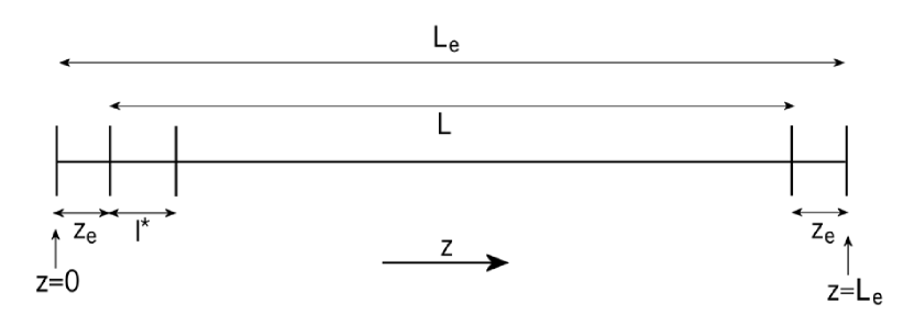
Figure 1: Notation used in derivations. $z$, $L$, $z_{e}$, $l^{*}$, and $L_{e}$ are the slab coordinate and size, an extrapolation length, the transport mean free path, and an effective width, respectively. Actual slab between coordinates $z_{e}$, and $L_{e}-z_{e}$.

For axial symmetric conditions, one can group cartesian coordinates into $z$ and $r_{\perp}$, the perpendicular distance to the symmetry axis. The conjugate coordinates for time and space will be $s$ and $k_{\perp}$ (in this last case, conjugate to the radial distance only).

The diffusion equation describing the propagation of the intensity distribution is:

$$\frac{\partial}{\partial t}I=D_{0}\frac{\partial^{2}}{\partial z^{2}}I+D_{0}\nabla_{\bot}^{2}I-\alpha I+S\mbox{,}$$ (1)

where the symmetry is emphasized by the explicit grouping of spatial coordinates. $I$ is the intensity distribution, and $D_{0}$, $\alpha$ and $S$ the diffusion coefficient, absorption coefficient and source term. The operator $\nabla_{\bot}^{2}$ refers only to the coordinates defining the perpendicular to the symmetry axis.

For easy reference, $I\equiv I\left(r_{\bot},z,t\right)$ and $I^{LF}\equiv I^{LF,2D}\left(k_{\bot},z,s\right)$. $I\left(r_{\bot},z,t\right)$ signals axial symmetry. $I^{LF,2D}$ is the Laplace-Fourier transform, with 2D emphasizing that a 2D spatial Fourier transform is implied.

The source term is now written $S\left(r_{\bot},z,t\right)=\delta\left(x\right)\delta\left(y\right)\delta\left(z-\left(l^{*}+z_{e}\right)\right)\delta\left(t\right)$ (unit production plus the diffusion approximation of the whole of the external initial perturbation being substituted for a single delta, a transport mean free path away from the sample enclosure wall; all observables will come out normalized relative to the overall strength of the external perturbation).

In Fourier-Laplace one is left with footnote1 :

$$\left[\frac{\partial^{2}}{\partial z^{2}}-\left(k_{\bot}^{2}+\frac{s+\alpha}{D_{0}}\right)\right]I^{LF}=-\frac{1}{\pi}\frac{1}{D_{0}}\delta\left(z-\left(l^{*}+z_{e}\right)\right)\mbox{.}$$ (2)

Using standard Dirichelet boundary conditions Zhu1991 ; Haskell1994 and the extrapolation length, $\left\{I\left(r_{\bot},z=0,t\right)=0,\,I\left(r_{\bot},z=L_{e},t\right)=0\right\}$  Akkermans2006 , one obtains the solution:

$$I^{LF} = \frac{1}{\pi}\frac{1}{D_{0}}\frac{1}{\sqrt{A}}\frac{\sinh\sqrt{A}\left(l^{*}+z_{e}\right)\sinh\sqrt{A}\left(L_{e}-z\right)}{\sinh\sqrt{A}L_{e}}$$ (3)

$$\;\mathrm{if}\,z<l^{*}+z_{e}\mbox{,}$$

$$I^{LF} = \frac{1}{\pi}\frac{1}{D_{0}}\frac{1}{\sqrt{A}}\frac{\sinh\sqrt{A}\left(L_{e}-\left(l^{*}+z_{e}\right)\right)\sinh\sqrt{A}z}{\sinh\sqrt{A}L_{e}}$$ (4)

$$\;\mathrm{if}\,z>l^{*}+z_{e}\mbox{,}$$

with $A\equiv k_{\bot}^{2}+\frac{s+\alpha}{D_{0}}$.

The goal is to obtain quantities directly amenable to measurement, in simple setups. The sought experimental observables are therefore the fluxes ($\Phi$) in the exit planes, imaged in reflection ($R$) or transmission ($T$):

$$\Phi \equiv -D_{0}\frac{\partial I}{\partial z}\mbox{,}$$ (5)

$$R \equiv -\Phi\left(z=z_{e},t\right)\mbox{,}$$ (6)

$$T \equiv \Phi\left(z=L_{e}-z_{e},t\right)\mbox{.}$$ (7)

One is left with

$$\Phi_{R}^{LF} = -\frac{1}{\pi}\frac{\sinh\sqrt{A}\left(l^{*}+z_{e}\right)\cosh\sqrt{A}\left(L_{e}-z_{e}\right)}{\sinh\sqrt{A}L_{e}}\mbox{,}$$ (8)

$$\Phi_{T}^{LF} = \frac{1}{\pi}\frac{\sinh\sqrt{A}\left(L_{e}-\left(l^{*}+z_{e}\right)\right)\cosh\sqrt{A}\left(L_{e}-z_{e}\right)}{\sinh\sqrt{A}L_{e}}\mbox{,}$$ (9)

whose Fourier-Lapace inversion gives:

$$T\left(r,t\right)=\frac{1}{2}\frac{1}{L_{e}^{2}}\frac{e^{-\frac{1}{4}\frac{r^{2}}{D_{0}t}}\,e^{-\alpha t}}{D_{0}t}\overset{+\infty}{\underset{n=1}{\sum}}\left(-1\right)^{n+1}\times$$ (10)

$$\times n\,\cos\left(n\pi\frac{z_{e}}{L_{e}}\right)\,\sin\left(n\pi\frac{l^{*}+z_{e}}{L_{e}}\right)\,e^{-n^{2}\pi^{2}\frac{D_{0}t}{L_{e}^{2}}}\mbox{,}$$

for the transmission time resolved profile. For the reflection a similar expression is obtained, the only difference being that the term $\left(-1\right)^{n+1}$ is absent. PLEASE NOTE that in all of the remaining manuscript it is shown only the Transmission results. The Reflection counterparts are obtained simply by omitting this term. This is done in order not to overload the manuscript.

The last equation is obtained by Laplace inverse transform in the complex plane (Bromwich integral with poles at $\sqrt{A}L_{e}=in\pi$) and Fourier inverse transform which, for axially symmetric functions, takes the simple form $f^{2D}\left(r\right)=\int_{0}^{+\infty}F^{2D}\left(k\right)J_{0}\left(kr\right)k\,dk$, using the zero order Bessel function Baddour2009 ; Baddour2011 .

Three further important observables are total intensity, integrated in space,  $T^{TOTAL}\left(t\right)=\int_{0}^{+\infty}\int_{0}^{2\pi}T\left(r,t\right)r\,d\theta dr$, the steady state radial profiles,  $T^{SS}\left(r\right)=\int_{0}^{+\infty}T\left(r,t\right)\,dt$, and the total signal also in steady state, obtained by spatial integrating the radial profiles $T^{SS,TOTAL}=\int_{0}^{+\infty}\int_{0}^{2\pi}T^{SS}\left(r\right)r\,d\theta dr$:

$$T^{TOTAL}\left(t\right)=\frac{2\pi}{L_{e}^{2}}e^{-\alpha t}\overset{+\infty}{\underset{n=1}{\sum}}\left(-1\right)^{n+1}\times$$ (11)

$$\times n\,\cos\left(n\pi\frac{z_{e}}{L_{e}}\right)\,\sin\left(n\pi\frac{l^{*}+z_{e}}{L_{e}}\right)\,e^{-n^{2}\pi^{2}\frac{D_{0}t}{L_{e}^{2}}}\mbox{,}$$

$$T^{SS}\left(r\right)=\frac{1}{L_{e}^{2}}\overset{+\infty}{\underset{n=1}{\sum}}\left(-1\right)^{n+1}\times$$ (12)

$$\times n\,\cos\left(n\pi\frac{z_{e}}{L_{e}}\right)\,\sin\left(n\pi\frac{l^{*}+z_{e}}{L_{e}}\right)\,\times$$

$$\times K_{0}\left(\sqrt{\frac{n^{2}\pi^{2}}{L_{e}^{2}}+\frac{\alpha}{D_{0}}}r\right)\mbox{,}$$

$$T^{SS,TOTAL}=\frac{2}{\pi}\overset{+\infty}{\underset{n=1}{\sum}}\left(-1\right)^{n+1}\times$$ (13)

$$\times\frac{1}{n\left(1+\frac{\alpha L_{e}^{2}}{D_{0}n^{2}\pi^{2}}\right)}\,\cos\left(n\pi\frac{z_{e}}{L_{e}}\right)\,\sin\left(n\pi\frac{l^{*}+z_{e}}{L_{e}}\right)\mbox{,}$$

where $K_{0}$ is the modified Bessel function of the second kind.

Eqs. (10-13) constitute the main contribution of this manuscript. Compare also the time resolved total (not spatial resolved) fluxes in refs. Maret2000 and Johnson2003 .

Please note that, without absorption ($\alpha=0$)

$$R^{SS,TOTAL}+T^{SS,TOTAL}=$$ (14)

$$= \frac{4}{\pi}\overset{+\infty}{\underset{n=0}{\sum}}\frac{1}{2n+1}\,\cos\left(\left(2n+1\right)\pi\frac{z_{e}}{L_{e}}\right)\,\times$$

$$\times\sin\left(\left(2n+1\right)\pi\frac{l^{*}+z_{e}}{L_{e}}\right)=1\mbox{,}$$

which express energy conservation (and is therefore a simple consistency check).

Eqs. (10-13) are best recast in dimensionless coordinates. The characteristic scales are:

$$r^{\prime} = \frac{r}{L_{e}}\mbox{,}$$ (15)

$$t^{\prime} = \frac{D_{0}t}{L_{e}^{2}}\mbox{,}$$ (16)

$$\alpha^{\prime} = \frac{L_{e}^{2}\alpha}{D_{0}}\mbox{,}$$ (17)

and the previous results become:

$$T\left(r^{\prime},t^{\prime}\right)\equiv\frac{T\left(r,t\right)}{\frac{1}{2D_{0}L_{e}}}=\frac{e^{-\frac{1}{4}\frac{r^{\prime 2}}{t^{\prime}}}\,e^{-\alpha^{\prime}t^{\prime}}}{t^{\prime}}\overset{+\infty}{\underset{n=1}{\sum}}\left(-1\right)^{n+1}\times$$ (18)

$$n\,\cos\left(n\pi\frac{z_{e}}{L_{e}}\right)\,\sin\left(n\pi\frac{l^{*}+z_{e}}{L_{e}}\right)\,e^{-n^{2}\pi^{2}t^{\prime}}\mbox{,}$$

$$T^{TOTAL}\left(t^{\prime}\right)\equiv\frac{T^{TOTAL}\left(t\right)}{\frac{2\pi}{D_{0}}}=e^{-\alpha^{\prime}t^{\prime}}\overset{+\infty}{\underset{n=1}{\sum}}\left(-1\right)^{n+1}\times$$ (19)

$$n\,\cos\left(n\pi\frac{z_{e}}{L_{e}}\right)\,\sin\left(n\pi\frac{l^{*}+z_{e}}{L_{e}}\right)\,e^{-n^{2}\pi^{2}t^{\prime}}\mbox{,}$$

$$T^{SS}\left(r^{\prime}\right)\equiv\frac{T^{SS}\left(r\right)}{\frac{1}{L_{e}}}=\overset{+\infty}{\underset{n=1}{\sum}}\left(-1\right)^{n+1}\times$$ (20)

$$n\,\cos\left(n\pi\frac{z_{e}}{L_{e}}\right)\,\sin\left(n\pi\frac{l^{*}+z_{e}}{L_{e}}\right)\,\times$$

$$K_{0}\left(\sqrt{n^{2}\pi^{2}+\alpha^{\prime}}r^{\prime}\right)\mbox{,}$$

$$T^{SS,TOTAL}=\frac{2}{\pi}\overset{+\infty}{\underset{n=1}{\sum}}\left(-1\right)^{n+1}\times$$ (21)

$$\frac{1}{n\left(1+\frac{\alpha^{\prime}}{n^{2}\pi^{2}}\right)}\,\cos\left(n\pi\frac{z_{e}}{L_{e}}\right)\,\sin\left(n\pi\frac{l^{*}+z_{e}}{L_{e}}\right)\mbox{.}$$

Two aspects are worth mentioning. The first is the asymptotic behaviour, in space and time. This is obtained in the previous equations making $n=1$, which is the slowest decaying term. The asymptotics are:

$$T\left(r^{\prime},t^{\prime}\right) \propto \frac{e^{-\frac{1}{4}\frac{r^{\prime 2}}{t^{\prime}}}\,e^{-\left(\pi^{2}+\alpha^{\prime}\right)t^{\prime}}}{t^{\prime}}\mbox{,}$$ (22)

$$T^{TOTAL}\left(t^{\prime}\right) \propto e^{-\left(\pi^{2}+\alpha^{\prime}\right)t^{\prime}}\mbox{,}$$ (23)

$$T^{SS}\left(r^{\prime}\right) \propto K_{0}\left(\sqrt{\pi^{2}+\alpha^{\prime}}r^{\prime}\right)\mbox{.}$$ (24)

The time-resolved distributions are Gaussian (with variance linear with time). The total signal, integrated in space, is exponential with $t^{\prime}$. And the steady state radial distributions are quasi-exponential with the radial distance $r^{\prime}$. This last statement is due to the facts Kaiser2014 ; Duffy2001 :  (1) $K_{\alpha}\left(x\right)=\frac{\pi}{2}i^{\alpha+1}H_{\alpha}^{(1)}\left(ix\right)$, for $-\pi<arg(x)\leq\pi$, and (2) $K_{0}\left(\sqrt{\pi^{2}+\alpha^{\prime}}r^{\prime}\right)\propto r^{\prime-1/2}exp\left(-\sqrt{\pi^{2}+\alpha^{\prime}}r^{\prime}\right)$. The $r^{\prime-1/2}$ has a much weaker dependence on the distance than the exponential, and a approximate exponential dependence follows.

The second aspect is the mean displacement, as can be judged from the radial profiles in reflection or transmission. It is well known that Brownian diffusion gives a mean square displacement that is linear with time in two dimensions. In fact, the time dependence of this mean square displacement is the most important parameter distinguishing classical from anomalous diffusion. It is therefore tempting to estimate the mean radial displacement, relative to the symmetry axis, in the imaged fluxes. The result is $\left\langle r^{\prime 2}\right\rangle\propto t^{\prime}$, showing that, the physical signature of classical diffusion survives in the imaged fluxes for the three dimensional slab (see also Akkermans2006 ; Maret2013 ; VanTiggelen2008 ).

Figs. 2 to 4 provide a graphical illustration of the results in eqs. (18-21). Fig. 2 shows the radial profiles, in steady state, illustrating the quasi-exponential radial asymptotic. This asymptotic regime was recently verified experimentally Kaiser2014 . Fig. 3 shows time resolved total transmission and reflection, illustrating also the asymptotics of eq. (23). Fig. 4 shows that the series in the previous equations reproduce the trend known for the diffusion in the slab: overall transmission in steady-state in inversely proportional to slab width, in the absence of absorption Akkermans2006 . It further shows that this scaling is broken, if absorption is present.

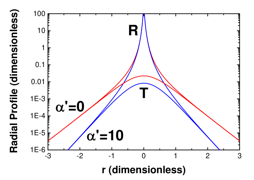
Figure 2: (Color online) Steady state radial profiles, in transmission (T) and reflection (R), using eq. (20) ($2000$ terms, $l^{*}=1$, $L_{e}=50$, $z_{e}=2/3l^{*}$). $\alpha^{\prime}$ is a normalized absorption coefficient.

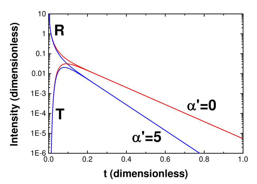
Figure 3: (Color online) Time resolved total intensity in transmission (T) and reflection (R), using eq. (20) ($2000$ terms, $l^{*}=1$, $L_{e}=50$, $z_{e}=2/3l^{*}$). $\alpha^{\prime}$ is a normalized absorption coefficient.

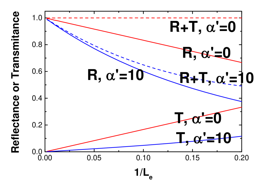
Figure 4: (Color online) Trnasmitance (T), reflectance (R) and sum (T+R), as a function of inverse efective slab width, using eq. (21) ($2000$ terms, $l^{*}=1$, $z_{e}=2/3l^{*}$). $\alpha^{\prime}$ is a normalized absorption coefficient. Without absorption, $R+T=1$ which is a manifestation of energy conservation.

One important aspect in the derivations was that the slab was considered infinite, in the transverse directions. The finite size could destroy the quasi-exponential asymptotics of the radial profiles. Reference Kaiser2014 gives empirical evidence that this asymptotic is amenable to experimental measurement, for an actual slab representative of simple experimental conditions (aspect ratio of slab diameter to width roughly $10$).

The spatial profiles in fig. 2 needed special care in their evaluation near the origin. The modified Bessel function of the second kind diverge at the origin. Although it is not provided an analytical proof of the series convergence, an empirical study of the series convergence was nevertheless conducted. Using a sufficient high number of terms, it was verified in all cases the series convergence. The convergence is however very slow. The fixed number of terms in fig. 2 correspond to a conservative estimate, based in the smallest distance considered (see also Kaiser2014 ).

III Inside of slab dynamics

The results presented thus far are focused in the dynamics of the transmission and reflection fluxes, since these are the ones most easily measured. The dynamics inside the slab is nevertheless of importance. The procedures used in the inverse Laplace and Fourier transforms of eqs. (8-9), can be equally applied to obtain the dynamics inside the slab. Eqs. (3-4) give, first for the dynamics in direct physical variables

$$I\left(r,z,t\right)=\frac{1}{2\pi L_{e}}\frac{e^{-\frac{1}{4}\frac{r^{2}}{D_{0}t}}\,e^{-\alpha t}}{D_{0}t}\overset{+\infty}{\underset{n=1}{\sum}}\sin\left(n\pi\frac{l^{*}+z_{e}}{L_{e}}\right)\,\times$$ (25)

$$\times\sin\left(n\pi\frac{z}{L_{e}}\right)\,e^{-n^{2}\pi^{2}\frac{D_{0}t}{L_{e}^{2}}}\mbox{,}$$

$$I^{SS}\left(r,z\right)=\frac{1}{\pi D_{0}L_{e}}\overset{+\infty}{\underset{n=1}{\sum}}\sin\left(n\pi\frac{l^{*}+z_{e}}{L_{e}}\right)\,\times$$ (26)

$$\times\sin\left(n\pi\frac{z}{L_{e}}\right)\,K_{0}\left(\sqrt{\frac{n^{2}\pi^{2}}{L_{e}^{2}}+\frac{\alpha}{D_{0}}}r\right)\mbox{,}$$

$$I^{SS,TOTAL}\left(z\right)=\frac{2}{\pi^{2}}\frac{L_{e}}{D_{0}}\overset{+\infty}{\underset{n=1}{\sum}}\frac{1}{n^{2}\left(1+\frac{\alpha L_{e}^{2}}{D_{0}n^{2}\pi^{2}}\right)}\,\times$$ (27)

$$\times\sin\left(n\pi\frac{l^{*}+z_{e}}{L_{e}}\right)\,\sin\left(n\pi\frac{z}{L_{e}}\right)\mbox{,}$$

and, then for its reformulation in dimensionless coordinates

$$I\left(r^{\prime},z,t^{\prime}\right)\equiv\frac{I\left(r,z,t\right)}{\frac{1}{2\pi D_{0}}}=\frac{e^{-\frac{1}{4}\frac{r^{\prime 2}}{t^{\prime}}}\,e^{-\alpha^{\prime}t^{\prime}}}{t^{\prime}}\times$$ (28)

$$\times\overset{+\infty}{\underset{n=1}{\sum}}\sin\left(n\pi\frac{l^{*}+z_{e}}{L_{e}}\right)\,\sin\left(n\pi\frac{z}{L_{e}}\right)\,e^{-n^{2}\pi^{2}t^{\prime}}\mbox{,}$$

$$I^{SS}\left(r^{\prime},z\right)\equiv\frac{I^{SS}\left(r,z\right)}{\frac{1}{\pi D_{0}}}=\overset{+\infty}{\underset{n=1}{\sum}}\sin\left(n\pi\frac{l^{*}+z_{e}}{L_{e}}\right)\,\sin\left(n\pi\frac{z}{L_{e}}\right)\,\times$$ (29)

$$\times K_{0}\left(\sqrt{n^{2}\pi^{2}+\alpha^{\prime}}r^{\prime}\right)\mbox{,}$$

$$\frac{I^{SS,TOTAL}\left(z\right)}{\frac{2}{\pi^{2}}\frac{L_{e}}{D_{0}}}=\overset{+\infty}{\underset{n=1}{\sum}}\frac{1}{n^{2}\left(1+\frac{\alpha^{\prime}}{n^{2}\pi^{2}}\right)}\,\times$$ (30)

$$\times\sin\left(n\pi\frac{l^{*}+z_{e}}{L_{e}}\right)\,\sin\left(n\pi\frac{z}{L_{e}}\right)\mbox{.}$$

Finally, fig. 5 represents the steady-state intensity inside the slab, integrated over radial distances, as a function of spatial coordinate. This result encompasses the known trend, for a unidimensional formulation of diffusion in absence of absorption: the intensity is linear in the difference to a coordinate inside the slab, situated one mean free path away from the boundary (this position comes from the approximation in the source term, the linear dependence comes from diffusion itself) Johnson2003 ; Maret2000 . It further quantifies to what extend absorption destroys the linear dependence with distance. The inset gives evidence that, at least for strong absorption, the dependence with distance can be reasonably approximated by an exponential (see also Akkermans2006 ).

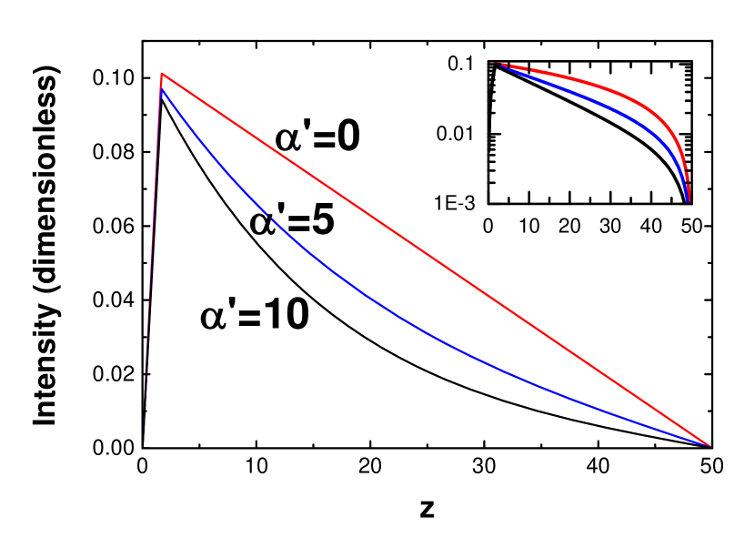
Figure 5: (Color online) Steady state intensity distribution inside slab, using eq. (30) ($2000$ terms, $l^{*}=1$, $L_{e}=50$, $z_{e}=2/3l^{*}$). Total intensity, integrated in a plane perpendicular to the $z$ coordinate. $\alpha^{\prime}$ is a normalized absorption coefficient. Actual slab between coordinates $z_{e}$, and $L_{e}-z_{e}$.

IV Conclusions

This contribution presents an analytical representation for the full dynamics in the simplest of the possible realizations of a diffusion process: classical diffusion of scalar waves in a fully developed multiple scattering regime, in an homogeneous plane-parallel slab. These conditions preserve axial symmetry, which was exploited in the derivations. The analytical series is strictly valid for a unit initial perturbation. However, under linear system response conditions, the convolution with the spatial and temporal distributions of the perturbation allow a solution for all other cases. Although this is conceptually trivial, even a numerical implementation of a 2D spatial convolution of two radial symmetric functions (initial external perturbation and system response) must implement a proper definition of the convolution as a two-dimensional convolution Baddour2011 . For other alternative approaches for taking into account the finite dimensions of the external perturbation see refs. Akkermans2006 ; Ishimaru1983 . Ref. Baddour2011 can additionally provide a basis for a generalization of this contribution to non axial symmetric situations.

It is expected that this contribution stimulates quantitative detailed comparison with experimental results, obtained in actual setups not amenable to a realistic unidimensional formulation of the geometry. Its main contribution is the derivation of the spatial resolved profiles, including absorption. These can help in obtaining unambiguous conclusions in reports of Anderson localization of classical waves in three dimensions, a subject of current interest and debate Maret2013 ; VanTiggelen2008 ; correspondence .

- (1) R. Klages, G. Radons, and I.N. Sokolov, eds., Anomalous Transport, Foundations and Applications (Wiley-VCH, 2008).
- (2) R.Metzler and J. Klafter, J. Phys. A 37, R161 (2004).
- (3) D. Mihalas, Stellar Atmospheres, 2nd Ed., (W.H. Freeman, 1978).
- (4) E. Akkermans and G. Montambaux, Mesoscopic Physics of Electrons and Photons (Cambridge University Press, 2006).
- (5) Q. Baudouin, R. Pierrat, A. Eloy, E.J. Nunes-Pereira, P.-A. Cuniasse, N. Mercadier, and R. Kaiser, Phys. Rev. E 90, 052114 (2014).
- (6) D.J. Durian, Phys. Rev. E 50, 857 (1994).
- (7) The constant term depends on the notation chosen to distribute constants over the direct and inverse transforms.
- (8) J.X. Zhu, D.J. Pine, and D.A. Weitz, Phys. Rev. A 44, 3948 (1991).
- (9) R.C. Haskell, L.O. Svaasand, T.-T. Tsay, T.-C. Feng, M.S. McAdams, and B.J. Tromberg, J. Opt. Soc. Am. A 11, 2727 (1994).
- (10) N. Baddour, J. Opt. Soc. Am. A 26, 1768 (2009).
- (11) N. Baddour, Two-Dimensional Fourier Transforms in Polar Coordinates, in P.W. Hawkes, ed., Advances in Imaging and Electron Physics, Vol. 165, (Elsevier, 2011).
- (12) R. Lenke and G. Maret, Multiple Scattering of Light: Coherent Backscattering and Transmission, in W. Brown and K. Mortensen, eds., Scattering in Polymeric and Colloidal Systems, (Gordon and Breach Scientific, 2000).
- (13) P.M. Johnson, A. Imhof, B.P.J. Bret, J.G. Rivas, and Ad Legendijk, Phys. Rev. E 68, 016604 (2003).
- (14) D. Duffy, Green’s Function with Applications (CRC, 2001).
- (15) T. Sperling, W. Bührer, C.M. Aegerter, and G. Maret, Nature Photon. 7, 48 (2013).
- (16) H. Hu, A. Strybulevych, J.H. Page, S.E. Skipetrov, and B.A. van Tiggelen, Nature Phys. 4, 945 (2008).
- (17) A. Ishimaru, Y. Kuga, R. Cheung, and K. Shimizu, J. Opt. Soc. Am. A 73, 131 (1983).
- (18) F. Scheffold and D. Wiersma, Nature Photon. 7, 934 (2013); G. Maret, T. Sperling, W. Bührer, A. Lubatsch, R. Franck, and C.M. Aegerter, Nature Photon. 7, 934 (2013).