Gabor Frames of Gaussian Beams for the Schrödinger equation

Abstract.

The present paper is devoted to the semiclassical analysis of linear Schrödinger equations from a Gabor frame perspective. We consider (time-dependent) smooth Hamiltonians with at most quadratic growth. Then we construct higher order parametrices for the corresponding Schrödinger equations by means of $\hbar$-Gabor frames, as recently defined by M. de Gosson, and we provide precise $L^{2}$-estimates of their accuracy, in terms of the Planck constant $\hbar$. Nonlinear parametrices, in the spirit of the nonlinear approximation, are also presented. Numerical experiments are exhibited to compare our results with the early literature.

1. Introduction

The goal of this paper is to construct asymptotic solutions for Schrödinger equations

(1) $$\begin{cases}i\hbar\partial_{t}u=\widehat{H(t)}u\\ u(0)=u_{0},\end{cases}$$

by means of Gabor frames in the semi-classical regime ($\hbar\to 0^{+})$. Here $t\in[0,T]$, the initial condition $u_{0}\in L^{2}(\mathbb{R}^{d})$ and the quantum Hamiltonian $\widehat{H(t)}$ is supposed to be the $\hbar$-Weyl quantization of the classical observable $H(t,X)$, with $X=(x,\xi)\in{\mathbb{R}^{2d}}$.

1.1. Literature overview

There are many results about asymptotic solutions for partial differential equations (PDE’s), especially when the initial value is a wave packet, i.e. it is well localized in the physical space and it oscillates with an approximately constant frequency. In particular, if the initial profile is Gaussian (a coherent state), the solution will be highly concentrated along the classical trajectory, according to the correspondence principle. Such a semi-classical analysis for Schrödinger-type equations were widely studied in several papers, see e.g. [6, 17, 19, 30, 31, 32, 39] and the textbooks [7, 27, 28, 29, 44].

The natural idea of this work is to decompose the initial value $u_{0}$ in (1) by means of a $\hbar$-Gabor frame whose atoms are Gaussian coherent states, construct asymptotic solutions for each of them, a so-called Gaussian beam, and finally by superposition obtain the asymptotic solution to (1). The main issues are the following:

• Construction of a parametrix via Gabor frames

• Estimates in $L^{2}$ for the parametrix and the error term

• Numerical results.

Despite the simplicity of the idea, we do not know a fully rigorous treatment of this matter. There are various attempts (see e.g. [2] and references therein) where however several arguments are carried out only at a heuristic level and with numerical experiments. The present paper is devoted to a rigorous study of these issues for a class of smooth Hamiltonians with at most quadratic growth and, unlike the previous work, we address from the beginning a finer analysis, that is higher order approximations: the approximate solution is searched as a (finite) sum of powers of $\hbar$, and the order of approximation can be arbitrarily large.

1.2. Notation and ($\hbar$-)Gabor frames

To be explicit, let us fix some notation.

The $\hbar$-Weyl quantization of a function $H$ on the phase space ${\mathbb{R}^{2d}}$ is formally defined by

(2) $$\widehat{H}u(x)=Op^{w}_{\hbar}[H]u(x)=(2\pi\hbar)^{-d}\int_{{\mathbb{R}^{2d}}}e^{i\hbar^{-1}(x-y)p}H\Big{(}\frac{x+y}{2},p\Big{)}u(y)\,dydp$$

for every $u$ in the Schwartz space $\mathcal{S}(\mathbb{R}^{d})$. The function $H$ is called the $\hbar$-Weyl symbol of $\widehat{H}$. For $z_{0}=(x_{0},p_{0})\in{\mathbb{R}^{2d}}$, we define by $\widehat{\mathcal{T}}^{\hbar}(z_{0})$ the Weyl operator

(3) $$\widehat{\mathcal{T}}^{\hbar}(z_{0})u(x)=Op^{w}_{\hbar}[e^{i\hbar^{-1}(p_{0}x-x_{0}p)}]u(x)=e^{i\hbar^{-1}(p_{0}x-x_{0}p_{0}/2)}u(x-x_{0}).$$

Such operator meets the definition of the so-called $\hbar$-Gabor frames, introduced in [19] as generalizations of Gabor frames. For a given lattice $\Lambda$ in ${\mathbb{R}^{2d}}$ and a non-zero square integrable function $\varphi$ (called window) on $\mathbb{R}^{d}$ the system

$$\mathcal{G}^{\hbar}(\varphi,\Lambda)=\{\widehat{\mathcal{T}}^{\hbar}(z)\varphi\,:\,z\in\Lambda\}$$

is called a $\hbar$-Gabor frame if it is a frame for $L^{2}(\mathbb{R}^{d})$, that is there exist constants $0<a\leq b$ such that

(4) $$a\|f\|_{2}^{2}\leq\sum_{z\in\Lambda}|\langle f,\widehat{\mathcal{T}}^{\hbar}(z)\varphi\rangle|^{2}\leq b\|f\|_{2}^{2},\quad\forall f\in L^{2}(\mathbb{R}^{d}).$$

In particular, when $\hbar=(2\pi)^{-1}$, the operator $\widehat{\mathcal{T}}(z_{0}):=\widehat{\mathcal{T}}^{(2\pi)^{-1}}(z_{0})$ is the so-called time-frequency (or phase-space) shift

$$\widehat{\mathcal{T}}(z_{0})f(x)=e^{-\pi ip_{0}x_{0}}e^{2\pi ip_{0}x}f(x-x_{0})=T_{x_{0}}M_{p_{0}}f(x),\quad z_{0}=(x_{0},p_{0}),$$

where translation and modulation operators are defined by

$$T_{x_{0}}f(x)=f(x-x_{0})\quad\mbox{and}\quad M_{p_{0}}f(x)=e^{2\pi ip_{0}x}f(x).$$

In this case we recapture the standard definition of a Gabor frame (see the next section for more details). Since they first appearance in the fundamental paper by Duffin and Schaffer [20] on non-uniform sampling of band-limited functions, frames have been applied in many fields of mathematics and physics. In particular, Gabor frames have been widely used in signal analysis, time-frequency analysis, quantum physics. Recently Gabor frames have been successfully applied in the study of PDE’s. In [9, 11] they have shown to provide optimally sparse representations for Schrödinger type propagators and in [13] reveal to be an equally efficient tool for representing solutions to hyperbolic and parabolic-type differential equations with constant coefficients. More generally, wave packet analysis and almost diagonalization of pseudodifferential and Fourier integral operators by Gabor frames have been performed in [10, 12, 14, 15, 16, 26, 35].

Pursuing the work on deformation of Gabor frames, that have been investigated by many authors [1, 8, 21, 25, 34], de Gosson in [19] uses the Schrödinger evolution to deform Gabor frames.

This paper is intended to be in some sense complementary to the work of de Gosson [19], because we use the frames to construct an approximate propagator for the Schrödinger equation. We also adopt almost the same notation as in [19].

1.3. Main Results

Here we consider $\hbar$-Gabor frames where the window function is the standard Gaussian

(5) $$\phi_{0}(x)=\pi^{-d/4}e^{-|x|^{2}/2}$$

and its rescaled version

(6) $$\phi^{\hbar}_{0}(x)=(\pi\hbar)^{-d/4}e^{-|x|^{2}/(2\hbar)}.$$

We define the coherent state centered at $z\in{\mathbb{R}^{2d}}$ the function

(7) $$\phi^{\hbar}_{z}(x)=\widehat{\mathcal{T}}^{\hbar}(z)\phi^{\hbar}_{0}(x).$$

Consider the solution $z_{t}=(x_{t},p_{t})$ to the Hamiltonian system

(8) $$\dot{x}_{t}=\partial_{p}H(t,x_{t},p_{t}),\quad\dot{p}_{t}=-\partial_{x}H(t,x_{t},p_{t})$$

with initial value $z_{0}=(x_{0},p_{0})$ and define

(9) $$H^{(2)}_{z_{0}}(t,X)=\sum_{|\gamma|=2}\frac{1}{\gamma!}\partial^{\gamma}_{X}H(t,z_{t})X^{\gamma},\quad X\in{\mathbb{R}^{2d}}.$$

It is well-known that the solution to the corresponding operator Schrödinger equation for $\hbar=1$

(10) $$i\partial_{t}\widehat{S_{t}}(z_{0})=Op^{w}_{1}[H^{(2)}_{z_{0}}(t)]\widehat{S_{t}}(z_{0})\quad\widehat{S_{0}}(z_{0})=I,$$

is a metaplectic operator $\widehat{S_{t}}(z_{0})$ corresponding to the symplectic matrix $S_{t}(z_{0})$ via the metaplectic representation [17, 39]. Following the works [30, 31, 39], a natural ansatz for asymptotic solutions to (1), modulo $O(\hbar^{(N+1)/2})$, $N\in\mathbb{R}$, where the initial value is the coherent state $\phi^{\hbar}_{z_{0}}$, that is

(11) $$\begin{cases}i\hbar\partial_{t}u=\widehat{H(t)}u\\ u(0)=\phi^{\hbar}_{z_{0}},\end{cases}$$

is provided by the Gaussian beam

(12) $$\phi^{\hbar,N}_{z_{0}}(x)=e^{\frac{i}{\hbar}\delta(t,z_{0})}\widehat{\mathcal{T}}^{\hbar}(z_{t})\widehat{M}_{\hbar^{-1/2}}\widehat{S_{t}}(z_{0})\sum_{j=0}^{N}\hbar^{j/2}b_{j}(t,x)\phi_{0}(x).$$

Here the symmetrized action $\delta$ is defined by

(13) $$\delta(t,z_{0})=\int_{0}^{t}\Big{(}\frac{1}{2}\sigma(z_{s},\dot{z}_{s})-H(s,z_{s})\Big{)}\,ds,$$

with $\sigma$ being the standard symplectic form; the metaplectic operator $\widehat{M}_{\hbar^{-1/2}}$ is given by

$$\widehat{M}_{\hbar^{-1/2}}f(x)=\hbar^{-d/4}f(\hbar^{-1/2}x)$$

and the functions $b_{j}(t,x)$ are suitable polynomials in $x$ with coefficients depending on $t,z_{0}$ ($b_{0}\equiv 1$), as we shall see in the sequel.

The construction of the parametrix via Gabor frames, having the previous Gaussian beams as building blocks, is performed as follows. Set

(14) $$h=2\pi\hbar,$$

and consider a $\hbar$-Gabor frame $\mathcal{G}^{\hbar}(\phi_{0}^{\hbar},h^{1/2}\Lambda)$ with $\Lambda=\alpha\mathbb{Z}^{d}\times\beta\mathbb{Z}^{d}$, $\alpha,\beta>0$. Let $\gamma^{h}$ be a dual window in $\mathcal{S}(\mathbb{R}^{d})$ (see the next section for details). For $N\geq 0$, $t\in[0,T]$, the parametrix to (1) is defined by

(15) $$[U^{(N)}(t)f](t,\cdot)=\sum_{z\in h^{1/2}\Lambda}\langle f,\widehat{\mathcal{T}}^{\hbar}(z)\gamma^{h}\rangle\phi_{z}^{\hbar,N}(t,\cdot).$$

Observe that $U^{(N)}(0)f=f$.

The following assumptions will be imposed throughout the paper.

Assumption (H). Suppose that the symbol $H(t,X)$ is continuous with respect to $(t,X)\in[0,T]\times{\mathbb{R}^{2d}}$ and smooth in $X$, satisfying

(16) $$|\partial^{\alpha}_{X}H(t,X)|\leq C_{\alpha},\quad\forall|\alpha|\geq 2,\ X\in{\mathbb{R}^{2d}},\ t\in[0,T].$$

This is our main result.

Theorem 1.1.

Under the Assumption (H) and with the above notation, there exists a constant $C=C(T)$ such that, for every $f\in L^{2}(\mathbb{R}^{d})$,

(17) $$\|U^{(N)}(t)f\|_{L^{2}(\mathbb{R}^{d})}\leq C\|f\|_{L^{2}(\mathbb{R}^{d})}\quad\forall t\in[0,T]$$

and

(18) $$\|(i\hbar\partial_{t}-\widehat{H(t)})U^{(N)}f\|_{L^{2}(\mathbb{R}^{d})}\leq C\hbar^{(N+3)/2}\|f\|_{L^{2}(\mathbb{R}^{d})}\quad\forall t\in[0,T].$$

If $U(t)$ denotes the exact propagator, for every $f\in L^{2}(\mathbb{R}^{d})$,

(19) $$\|(U^{(N)}(t)-U(t))f\|_{L^{2}(\mathbb{R}^{d})}\leq Ct\hbar^{(N+1)/2}\|f\|_{L^{2}(\mathbb{R}^{d})}\quad\forall t\in[0,T].$$

The pioneering papers in this spirit, for Hamiltonians $H(t,x,p)=V(x)+p^{2}/2$, come back to [30, 31]. More general Hamiltonians were considered in [7, 39], which inspired this work.

In the framework of nonlinear approximation we can also consider nonlinear parametrices, constructed as follows.

Let $\eta\geq 0$ be a threshold, and for $f\in L^{2}(\mathbb{R}^{d})$ consider the index set

$$A_{\eta,f}=\{z\in h^{1/2}\Lambda:|\langle f,\widehat{\mathcal{T}}^{\hbar}(z)\gamma^{h}\rangle|>\eta\},$$

and the nonlinear operator

$$U^{(N)}_{\eta}(t)[f](t,\cdot)=\sum_{z\in A_{\eta,f}}\langle f,\widehat{\mathcal{T}}^{\hbar}(z)\gamma^{h}\rangle\phi_{z}^{\hbar,N}(t,\cdot).$$

In particular, for $\eta=0$ we recover $U^{(N)}(t)$.

In this case we attain the following issue.

Theorem 1.2.

Under the Assumption (H) and with the above notation, there exists a constant $C=C(T)>0$ such that, for every $f\in L^{2}(\mathbb{R}^{d})$, $\eta\geq 0$,

(20) $$\|U^{(N)}_{\eta}(t)[f]\|_{L^{2}(\mathbb{R}^{d})}\leq C\Big{(}\sum_{z\in A_{\eta,f}}|\langle f,\widehat{\mathcal{T}}^{\hbar}(z)\gamma^{h}\rangle|^{2}\Big{)}^{1/2}\quad\forall t\in[0,T]$$

and

(21) $$\|(i\hbar\partial_{t}-\widehat{H(t)})U^{(N)}_{\eta}[f]\|_{L^{2}(\mathbb{R}^{d})}\leq C\hbar^{(N+3)/2}\Big{(}\sum_{z\in A_{\eta,f}}|\langle f,\widehat{\mathcal{T}}^{\hbar}(z)\gamma^{h}\rangle|^{2}\Big{)}^{1/2}\quad\forall t\in[0,T].$$

If $U(t)$ denotes the exact propagator, for every $f\in L^{2}(\mathbb{R}^{d})$,

(22) $$\|U^{(N)}_{\eta}(t)[f]-U(t)f\|_{L^{2}(\mathbb{R}^{d})}\leq C\Big{(}\sum_{z\not\in A_{\eta,f}}|\langle f,\widehat{\mathcal{T}}^{\hbar}(z)\gamma^{h}|^{2}\Big{)}^{1/2}\\ +Ct\hbar^{(N+1)/2}\Big{(}\sum_{z\in A_{\eta,f}}|\langle f,\widehat{\mathcal{T}}^{\hbar}(z)\gamma^{h}\rangle|^{2}\Big{)}^{1/2}\ \forall t\in[0,T].$$

A similar nonlinear parametrix was constructed in [36] in the case $N=0$. In particular, the estimate (21) already appeared there (Theorem 5.1), but with an additional factor $\sqrt{|A_{\eta,f}|}$ in the righ-hand side: that estimate blows up when $\eta\to 0$ if $f$ has an infinite number of non zero Gabor coefficients (i.e. $|A_{0,f}|=+\infty$), whereas we see that this is not the case in (21). In addition, the parametrix in [36] was constructed by means of a truncated Gaussian, which introduces a further error in the estimate.

As a byproduct of these techniques, in Section 4 we will also extend the weak deformation of frames result in [19, Proposition 18] to the case of higher order deformations. However, since the approach is perturbative in nature, our result just holds for $t\hbar^{1/2}$ small enough, and no longer for every $t$ as in [19].

We end up by recalling that Gaussian beam methods have been employed to obtain asymptotic solutions to hyperbolic PDE’s in [38] and hyperbolic systems in [2, 3, 33, 37, 42, 43].

1.4. Numerical Results

Finally, in Section 5 we provide some numerical experiments. We study the Cauchy problem (1) for an Hamiltonian function $H(t,x,p)$ of the form

(23) $$H(t,x,p)=V(x)+\frac{p^{2}}{2},$$

with an oscillating potential. This is a standard setting for the so-called generalized harmonic oscillator and it is perfectly suited to discuss the behavior of the method in the presence of a potential hill and a potential well.

We develop numerical algorithms using MATLAB and the powerful LTFAT package, see [40, 41]. We address the long time propagation of the beams using the reinitialization procedure described in [36].

2. Preliminaries and time-frequency analysis tools

We refer to [23] for an introduction to time-frequency concepts and in particular to [17] for applications to Mathematical Physics. For sake of brevity, sometimes we write $xy=x\cdot y$, the scalar product on $\mathbb{R}^{d}$ and $|t|^{2}=t\cdot t$, for $t\in\mathbb{R}^{d}$. The brackets $\langle f,g\rangle$ denote the inner product of $L^{2}(\mathbb{R}^{d})$, i.e. $\langle f,g\rangle=\int f(t){\overline{g(t)}}dt$ and $\|f\|_{2}^{2}=\langle f,f\rangle$. The Schwartz class is denoted by $\mathcal{S}(\mathbb{R}^{d})$. For $1\leq p<\infty$, the space $\ell^{p}(\Lambda)$ is the space of sequences $a=\{{a}_{\lambda}\}_{\lambda\in\Lambda}$ on a lattice $\Lambda$, such that

$$\|a\|_{\ell^{p}}:=\left(\sum_{\lambda\in\Lambda}|a_{\lambda}|^{p}\right)^{1/p}<\infty.$$

We write ${\rm Sp}(d,\mathbb{R})$ for the group of symplectic matrices on ${\mathbb{R}^{2d}}$, i.e., $\mathcal{A}\in{\rm Sp}(d,\mathbb{R})$ if $\mathcal{A}$ is a $2d\times 2d$ invertible matrix such that $\mathcal{A}^{T}J\mathcal{A}=J$, where

(24) $$J=\begin{pmatrix}0_{d}&I_{d}\\ -I_{d}&0_{d}\end{pmatrix}.$$

The standard symplectic form on ${\mathbb{R}^{2d}}$ is

(25) $$\sigma(z,z^{\prime})=\;(z^{\prime})^{T}Jz,\qquad z,z^{\prime}\in\mathbb{R}^{2d}.$$

The metaplectic group is denoted by $Mp(d)$. Consider $\widehat{S}\in Mp(d)$ with covering projection $\pi^{\hbar}:\widehat{S}\mapsto S\in{\rm Sp}(d,\mathbb{R})$. The appearance of the subscript $\hbar$ is due to the fact that to the $\hbar$-dependent operator $\widehat{V}_{P}f(x)=e^{-iPx\cdot x/(2\hbar)}f(x)$ (chirp) corresponds the projection $\pi^{\hbar}(\widehat{V}_{P})=V_{P}$, with $V_{P}=\begin{pmatrix}I_{d}&0_{d}\\ -P&0_{d}\end{pmatrix}$, $P=P^{T}$, and to the Fourier transform $\widehat{J}f(x)=(2\pi i\hbar)^{-d/2}\int_{\mathbb{R}^{d}}e^{-ixx^{\prime}/\hbar}f(x^{\prime})\,dx^{\prime}$ corresponds $\pi^{\hbar}(\widehat{J})=J$, defined in (24). For details see [19, Appendix A] and the books [17, 18]. In particular, for $\lambda>0$ we shall use the metaplectic operator $\widehat{M}_{\lambda}\in Mp(d)$ defined (up to a sign) by

(26) $$\widehat{M}_{\lambda}f(x)=\lambda^{d/2}f(\lambda x),\,\quad f\in L^{2}(\mathbb{R}^{d})$$

and whose projection is $\pi^{\hbar}(\widehat{M}_{\lambda})=M_{\lambda}$, the symplectic matrix

(27) $$M_{\lambda}=\begin{pmatrix}\lambda^{-1}I_{d}&0_{d}\\ 0_{d}&\lambda I_{d}.\end{pmatrix}$$

In the sequel we shall often use the fundamental symplectic covariance formula

(28) $$\widehat{\mathcal{T}}^{\hbar}(z)\widehat{S}=\widehat{S}\widehat{\mathcal{T}}^{\hbar}(S^{-1}z)\quad S\in{\rm Sp}(d,\mathbb{R}).$$

2.1. $\hbar$-Gabor Frames

The definition of a $\hbar$-Gabor frame is already contained in the introduction. Consider a lattice $\Lambda$ in ${\mathbb{R}^{2d}}$. The Gabor system

$$\mathcal{G}(\varphi,\Lambda)=\{\widehat{\mathcal{T}}(z)\varphi,z\in\Lambda\},$$

(recall that $\widehat{\mathcal{T}}(z)=\widehat{\mathcal{T}}^{(2\pi)^{-1}}(z)$) is a Gabor frame for $L^{2}(\mathbb{R}^{d})$ if there exist constants $a,b>0$ such that for every $f\in L^{2}(\mathbb{R}^{d})$

(29) $$a\|f\|^{2}_{2}\leq\sum_{z\in\Lambda}|\langle f,\widehat{\mathcal{T}}(z)\varphi|^{2}\leq b\|f\|^{2}_{2}.$$

If $\eqref{Frame_rel}$ holds, then there exists a $\gamma\in L^{2}(\mathbb{R}^{d})$ (so-called dual window), such that $\mathcal{G}(\gamma,\Lambda)$ is a frame for $L^{2}(\mathbb{R}^{d})$ and every $f\in L^{2}(\mathbb{R}^{d})$ can be expanded as

(30) $$f=\sum_{z\in\Lambda}\langle f,\widehat{\mathcal{T}}(z)\varphi\rangle\widehat{\mathcal{T}}(z)\gamma=\sum_{z\in\Lambda}\langle f,\widehat{\mathcal{T}}(z)\gamma\rangle\widehat{\mathcal{T}}(z)\varphi,$$

with unconditional convergence in $L^{2}(\mathbb{R}^{d})$. In particular, if the window $\varphi$ is a Gaussian function, then there exists a dual window $\gamma$ that is smooth and well-localized, in particular $\gamma\in\mathcal{S}(\mathbb{R}^{d})$ (see [13, 24]).

In what follows we investigate some useful properties which let us switch from a $\hbar$-Gabor frame to a standard Gabor frame and vice-versa. To reach this goal, we define the dilation matrix $D^{\hbar}$ and its inverse $(D^{\hbar})^{-1}$

(31) $$D^{\hbar}=\begin{pmatrix}I_{d}&0_{d}\\ 0_{d}&hI_{d}.\end{pmatrix}\quad(D^{\hbar})^{-1}=\begin{pmatrix}I_{d}&0_{d}\\ 0_{d}&h^{-1}I_{d}\end{pmatrix}$$

(recall that $h=2\pi\hbar$).

Proposition 2.1.

Let $D^{\hbar}$ be the matrix defined in (31). The system $\mathcal{G}^{\hbar}(\varphi,\Lambda)$ is a $\hbar$-Gabor frame if and only if $\mathcal{G}(\varphi,(D^{\hbar})^{-1}\Lambda)$ is a Gabor frame and the frame bounds are the same. Moreover, every dual window $\gamma$ of the Gabor frame $\mathcal{G}(\varphi,(D^{\hbar})^{-1}\Lambda)$ originates a $\hbar$-Gabor frame $\mathcal{G}^{\hbar}(\gamma,\Lambda)$, dual frame of $\mathcal{G}^{\hbar}(\varphi,\Lambda)$.

Proof.

The first part is straightforward and follows the pattern of [19, Prop. 7]. Precisely, the system $\mathcal{G}^{\hbar}(\varphi,\Lambda)$ is a $\hbar$-Gabor frame if and only if there exist positive constants $a,b>0$ such that (4) holds. Setting $z=(x,2\pi\hbar p)\in\Lambda$ if and only if $(x,p)\in(D^{\hbar})^{-1}\Lambda$, and using $\widehat{\mathcal{T}}^{\hbar}(x,2\pi\hbar p)=\widehat{\mathcal{T}}(x,p)$, the inequalities (4) are equivalent to

$$a\|f\|_{2}^{2}\leq\sum_{z\in(D^{\hbar})^{-1}\Lambda}|\langle f,\widehat{\mathcal{T}}\varphi\rangle|^{2}\leq b\|f\|_{2}^{2},\quad\forall f\in L^{2}(\mathbb{R}^{d}),$$

as desired.

Now, consider a dual window $\gamma\in L^{2}(\mathbb{R}^{d})$ of the Gabor frame $\mathcal{G}(\varphi,(D^{\hbar})^{-1}\Lambda)$. Then every $f\in L^{2}(\mathbb{R}^{d})$ can be expanded as

$$f =\sum_{z\in(D^{\hbar})^{-1}\Lambda}\langle f,\widehat{\mathcal{T}}(z)\varphi\rangle\widehat{\mathcal{T}}(z)\gamma$$

$$=\sum_{(x,p)\in(D^{\hbar})^{-1}\Lambda}\langle f,\widehat{\mathcal{T}}^{\hbar}(x,2\pi\hbar p)\varphi\rangle\widehat{\mathcal{T}}^{\hbar}(x,2\pi\hbar p)\gamma$$

$$=\sum_{(x,p^{\prime})\in\Lambda}\langle f,\widehat{\mathcal{T}}^{\hbar}(x,p^{\prime})\varphi\rangle\widehat{\mathcal{T}}^{\hbar}(x,p^{\prime})\gamma,$$

that is the system $\{\widehat{\mathcal{T}}^{\hbar}(z),\,z\in\Lambda\}$ is a dual frame of the $\hbar$-Gabor frame $\mathcal{G}^{\hbar}(\varphi,\Lambda)$.

     

Given the Gaussian window $\phi_{0}$ defined in (5) and the lattice $\Lambda=\alpha\mathbb{Z}^{d}\times\beta\mathbb{Z}^{d}$, with $\alpha,\beta>0$, de Gosson in [19, Prop. 12] shows that the system $\mathcal{G}^{\hbar}(\phi_{0}^{\hbar},h^{1/2}\,\Lambda)$ is a $\hbar$-Gabor frame if and only if $\alpha\beta<1$, this means by the previous proposition that the system

(32) $$\mathcal{G}(\phi_{0}^{\hbar},\alpha h^{1/2}\,\mathbb{Z}^{d}\times\beta h^{-1/2}\mathbb{Z}^{d})$$

is a Gabor frame if and only if $\alpha\beta<1$. This frame will be used for the numerical experiments in Section 5.

Using the same arguments as in the proof of Proposition 2.1 we obtain the following characterization:

Proposition 2.2.

Let $D^{\hbar}$ be the matrix defined in (31) and consider a Gabor frame $\mathcal{G}(\varphi,\Lambda)$. The system $\mathcal{G}(\gamma,\Lambda)$ is a dual Gabor frame of $\mathcal{G}(\varphi,\Lambda)$ if and only if $\mathcal{G}^{\hbar}(\gamma,D^{\hbar}\Lambda)$ is a dual $\hbar$-Gabor frame of the $\hbar$-Gabor frame $\mathcal{G}^{\hbar}(\varphi,D^{\hbar}\Lambda)$. Moreover, the frame bounds of $\mathcal{G}(\varphi,\Lambda)$ and $\mathcal{G}^{\hbar}(\varphi,D^{\hbar}\Lambda)$ are the same.

We shall work with $\hbar$-Gabor frames where both windows and lattices are rescaled. Their dual frames behave as follows. We set

(33) $$\varphi^{h}(x)=h^{-d/4}\varphi(h^{-1/2}x)=\widehat{M}_{h^{-1/2}}\varphi(x)=\widehat{M}_{(2\pi\hbar)^{-1/2}}\varphi(x).$$

Proposition 2.3.

Consider a Gabor frame $\mathcal{G}(\varphi,\Lambda)$. The system $\mathcal{G}(\gamma,\Lambda)$ is a dual Gabor frame of $\mathcal{G}(\varphi,\Lambda)$ if and only if $\mathcal{G}^{\hbar}(\gamma^{h},h^{1/2}\,\Lambda)$ is a dual $\hbar$-Gabor frame of the $\hbar$-Gabor frame $\mathcal{G}^{\hbar}(\varphi^{h},h^{1/2}\,\Lambda)$. Moreover, the frame bounds of $\mathcal{G}(\varphi,\Lambda)$ and $\mathcal{G}^{\hbar}(\varphi^{h},h^{1/2}\,\Lambda)$ are the same.

Proof.

Consider the metaplectic operator $\widehat{M}_{h^{-1/2}}\in Mp(d)$ and its inverse $\widehat{M}_{h^{1/2}}\in Mp(d)$. For every $f\in L^{2}(\mathbb{R}^{d})$, we have $\widehat{M}_{h^{-1/2}}\widehat{M}_{h^{1/2}}f=f$. Given the Gabor frame $\mathcal{G}(\varphi,\Lambda)$ with dual Gabor frame $\mathcal{G}(\gamma,\Lambda)$, by Proposition 2.2 and using the boundedness of the metaplectic operators on $L^{2}(\mathbb{R}^{d})$ we can write, for every $f\in L^{2}(\mathbb{R}^{d})$,

$$f =\widehat{M}_{h^{-1/2}}\sum_{z\in D^{\hbar}\Lambda}\langle\widehat{M}_{h^{1/2}}f,\widehat{\mathcal{T}}^{\hbar}(z)\varphi\rangle\widehat{\mathcal{T}}^{\hbar}(z)\gamma$$

$$=\widehat{M}_{h^{-1/2}}\sum_{z\in h^{1/2}\,\Lambda}\langle\widehat{M}_{h^{1/2}}f,\widehat{\mathcal{T}}^{\hbar}(M_{h^{1/2}}\,z)\varphi\rangle\widehat{\mathcal{T}}^{\hbar}(M_{h^{1/2}}\,z)\gamma$$

$$=\sum_{z\in h^{1/2}\,\Lambda}\langle f,\widehat{M}_{h^{-1/2}}\widehat{\mathcal{T}}^{\hbar}(M_{h^{1/2}}\,z)\varphi\rangle\widehat{M}_{h^{-1/2}}\widehat{\mathcal{T}}^{\hbar}(M_{h^{1/2}}\,z)\gamma,$$

$$=\sum_{z\in h^{1/2}\,\Lambda}\langle f,\widehat{\mathcal{T}}^{\hbar}(z)\varphi^{h}\rangle\widehat{\mathcal{T}}^{\hbar}(z)\gamma^{h},$$

where we used $\widehat{\mathcal{T}}^{\hbar}(z)\widehat{M}_{h^{-1/2}}=\widehat{M}_{h^{-1/2}}\widehat{\mathcal{T}}^{\hbar}(M_{h^{1/2}}\,z)$, by the covariance formula (28) and the definition (33). This ends the proof of the equivalence of the dual frames. The proof of the frame bounds follows the argument of the first part of the proof of Proposition 2.1.      

3. Bounds for the parametrix in $L^{2}$

3.1. Preliminary remarks

We assume for the Hamiltonian $H(t,X)$ the validity of Assumption (H). In particular, we consider its second order Taylor term $H^{(2)}_{z_{0}}$ at $z_{0}=(x_{0},p_{0})$, as in (9) and the corresponding propagator $\widehat{S_{t}}(z_{0})$ in (10). We can also consider the operator $\widehat{S_{t}}^{\hbar}(z_{0})$ defined by

(34) $$i\hbar\partial_{t}\widehat{S_{t}}^{\hbar}(z_{0})=\widehat{H^{(2)}_{z_{0}}(t)}\widehat{S_{t}}^{\hbar}(z_{0})\quad\widehat{S_{0}}^{\hbar}(z_{0})=I.$$

This operator is related to $\widehat{S_{t}}$ via the formula (omitting the dependence on $z_{0}$ for simplicity)

$$\widehat{S_{t}}^{\hbar}=\widehat{M}_{\hbar^{-1/2}}\widehat{S_{t}}\widehat{M}_{\hbar^{1/2}}.$$

Indeed we have

$$i\hbar\widehat{S_{t}}^{\hbar} =i\hbar\partial_{t}\widehat{M}_{\hbar^{-1/2}}\widehat{S_{t}}\widehat{M}_{\hbar^{1/2}}$$

$$=\hbar\widehat{M}_{\hbar^{-1/2}}{\rm Op}^{w}_{1}[H^{(2)}(t,x,p)]\widehat{S_{t}}\widehat{M}_{\hbar^{1/2}}$$

$$=\hbar{\rm Op}^{w}_{1}[H^{(2)}(t,\hbar^{-1/2}x,\hbar^{1/2}p)]\widehat{M}_{\hbar^{-1/2}}\widehat{S_{t}}\widehat{M}_{\hbar^{1/2}}$$

$$={\rm Op}^{w}_{1}[H^{(2)}(t,x,\hbar p)]\widehat{S_{t}}^{\hbar}$$

$$=\widehat{H^{(2)}(t)}\widehat{S_{t}}^{\hbar}.$$

Remark 3.1.

The action of $\widehat{S_{t}}(z_{0})$ or $\widehat{S_{t}}^{\hbar}(z_{0})$ on a mudulated Gaussian function can be written down explicitly, for details we refer to Section 5 and the references quoted there.

Remark 3.2.

The projection $S_{t}(z_{0})$ represents the flow of the linear system with Hamiltonian $H^{(2)}_{z_{0}}(t,X)$. As a matrix, $S_{t}(z_{0})$ is in ${\rm Sp}(d,\mathbb{R})$, for every $t\in[0,T]$. The entries of the matrix $S_{t}(z_{0})$ depend on $t\in[0,T]$ and $z_{0}\in{\mathbb{R}^{2d}}$ but they are bounded, because this is true for the coefficients of the polynomial $H^{(2)}_{z_{0}}(t,X)$ by the assumption (16). The same is true for the entries of the inverse matrix $S_{t}^{-1}(z_{0})$.

3.2. Evolution of a coherent state

Consider the Cauchy problem (11). Let $z_{t}$ be the trajectory of the corresponding Hamiltonian system, with initial condition $z_{0}$. We will show that an approximate solution (Gaussian beam) is given by

(35) $$\phi^{\hbar,0}_{z_{0}}(t,\cdot) =e^{\frac{i}{\hbar}\delta(t,z_{0})}\widehat{\mathcal{T}}^{\hbar}(z_{t})\widehat{S_{t}}^{\hbar}(z_{0})\phi^{\hbar}_{0}$$

$$=e^{\frac{i}{\hbar}\delta(t,z_{0})}\widehat{\mathcal{T}}^{\hbar}(z_{t})\widehat{M}_{\hbar^{-1/2}}\widehat{S_{t}}(z_{0})\widehat{M}_{\hbar^{1/2}}\phi^{\hbar}_{0}$$

$$=e^{\frac{i}{\hbar}\delta(t,z_{0})}\widehat{\mathcal{T}}^{\hbar}(z_{t})\widehat{M}_{\hbar^{-1/2}}\widehat{S_{t}}(z_{0})\phi_{0},$$

where $\delta(t,z_{0})$ is the symmetrized action defined in (13). More generally, we will consider higher order approximations $\phi^{\hbar,N}_{z_{0}}(t)$ in the form (12).

To this end we will have to estimate the remainder term

(36) $$R^{(N)}_{z_{0}}(t,\cdot):=(i\hbar\partial_{t}-\widehat{H(t)})\phi^{\hbar,N}_{z_{0}}(t,\cdot).$$

The following computation of $R^{(N)}_{z_{0}}$ were carried out in [30, 31] for Hamiltonians of the form $H(t,x,p)=V(x)+p^{2}/2$ and in [7, 39] for more general Hamiltonians with polynomial growth. Here we briefly sketch the main points for the benefit of the reader, because the formula given in [39, (70)] for $R^{(N)}_{z_{0}}$ contains a number of misprints. An explicit computation show that

(37) $$i\hbar\partial_{t}e^{\frac{i}{\hbar}\delta(t,z_{0})} =-e^{\frac{i}{\hbar}\delta(t,z_{0})}\Big{(}\frac{1}{2}\sigma(z_{t},\dot{z}_{t})-H(t,z_{t})\Big{)}$$

$$=-e^{\frac{i}{\hbar}\delta(t,z_{0})}\Big{(}\frac{1}{2}(p_{t}\dot{x_{t}}-\dot{p_{t}}x_{t})-H(t,z_{t})\Big{)}.$$

On the other hand, given a function $f(x)$ we have

(38) $$i\hbar\partial_{t}\widehat{\mathcal{T}}^{\hbar}(z_{t})f(x) =e^{\frac{i}{\hbar}(p_{t}x-x_{t}p_{t}/2)}\Big{(}(-\dot{p_{t}}x+\frac{\dot{p_{t}}x_{t}+p_{t}\dot{x_{t}}}{2})f(x-x_{t})-i\hbar\dot{x_{t}}\nabla f(x-x_{t})\Big{)}$$

$$=\widehat{\mathcal{T}}^{\hbar}(z_{t})\Big{(}-\dot{p_{t}}x-\dot{p_{t}}x_{t}+\frac{\dot{p_{t}}x_{t}+p_{t}\dot{x_{t}}}{2}-i\hbar\dot{x_{t}}\nabla\Big{)}f(x)$$

$$=\widehat{\mathcal{T}}^{\hbar}(z_{t})\Big{(}\frac{p_{t}\dot{x_{t}}-\dot{p_{t}}x_{t}}{2}+x\partial_{x}H(t,z_{t})+\hbar\partial_{p}H(t,z_{t})(-i\nabla)\Big{)}f(x),$$

which implies

(39) $$i\hbar\partial_{t}\widehat{\mathcal{T}}^{\hbar}(z_{t})\widehat{M}_{\hbar^{-1/2}}\\ =\widehat{\mathcal{T}}^{\hbar}(z_{t})\widehat{M}_{\hbar^{-1/2}}\Big{[}i\hbar\partial_{t}+\frac{p_{t}\dot{x_{t}}-\dot{p_{t}}x_{t}}{2}+\hbar^{1/2}x\partial_{x}H(t,z_{t})+\hbar^{1/2}\partial_{p}H(t,z_{t})(-i\nabla)\Big{]}.$$

We also have the covariance formula

$$\widehat{H(t)}\widehat{\mathcal{T}}^{\hbar}(z_{t})=\widehat{\mathcal{T}}^{\hbar}(z_{t}){\rm Op}^{w}_{1}[H(t,x+x_{t},\hbar(p+\hbar^{-1}p_{t})]$$

which implies

(40) $$\widehat{H(t)}\widehat{\mathcal{T}}^{\hbar}(z_{t})\widehat{M}_{\hbar^{-1/2}}=\widehat{\mathcal{T}}^{\hbar}(z_{t})\widehat{M}_{\hbar^{-1/2}}{\rm Op}^{w}_{1}[H(t,h^{1/2}x+x_{t},\hbar^{1/2}p+p_{t})].$$

Finally a Taylor expansion yields

(41) $$H(t,\hbar^{1/2}x+x_{t},\hbar^{1/2}p+p_{t})=H(t,z_{t})+\hbar^{1/2}x\partial_{x}H(t,z_{t})+\hbar^{1/2}p\partial_{p}H(t,z_{t})\\ +\hbar H^{(2)}_{z_{0}}(t,X)+\sum_{l=3}^{N+2}\hbar^{l/2}H^{(l)}_{z_{0}}(t,X)+\hbar^{(N+3)/2}r^{(N+3)}_{z_{0}}(t,X),$$

where

$$H^{(l)}_{z_{0}}(t,X)=\sum_{|\gamma|=l}\frac{1}{\gamma!}\partial^{\gamma}_{X}H(t,z_{t})X^{\gamma},\quad X\in{\mathbb{R}^{2d}}$$

and

$$r^{(N+3)}_{z_{0}}(t,X)=\frac{1}{(N+3)!}\sum_{|\gamma|=N+3}\int_{0}^{1}\partial^{\gamma}_{X}H(t,z_{t}+\theta\hbar^{1/2}X)X^{\gamma}(1-\theta)^{N+2}\,d\theta.$$

By the formulas (37)–(41) we obtain

$$(i\hbar\partial_{t}-\widehat{H(t)})\phi^{\hbar,N}_{z_{0}}(t,\cdot)=e^{\frac{i}{\hbar}\delta(t,z_{0})}\widehat{\mathcal{T}}^{\hbar}(z_{t})\widehat{M}_{\hbar^{-1/2}}\Big{(}i\hbar\partial_{t}-\hbar{\rm Op}^{w}_{1}[H^{(2)}_{z_{0}}(t,X)]$$

$$-\sum_{l=3}^{N+2}\hbar^{l/2}{\rm Op}^{w}_{1}[H^{(l)}_{z_{0}}(t,X)]-\hbar^{(N+3)/2}{\rm Op}^{w}_{1}[r^{(N+3)}_{z_{0}}(t,X)])\Big{)}\widehat{S_{t}}(z_{0})\sum_{j=0}^{N}\hbar^{j/2}b_{j}(t,\cdot)\phi_{0}$$

$$=e^{\frac{i}{\hbar}\delta(t,z_{0})}\widehat{\mathcal{T}}^{\hbar}(z_{t})\widehat{M}_{\hbar^{-1/2}}\widehat{S_{t}}(z_{0})\Big{(}i\hbar\partial_{t}-\sum_{l=3}^{N+2}\hbar^{l/2}{\rm Op}^{w}_{1}[H^{(l)}_{z_{0}}(t,S_{t}(X))]$$

$$\qquad\qquad\qquad\qquad\qquad\quad-\hbar^{(N+3)/2}{\rm Op}^{w}_{1}[r^{(N+3)}_{z_{0}}(t,S_{t}(X))]\Big{)}\sum_{j=0}^{N}\hbar^{j/2}b_{j}(t,\cdot)\phi_{0}.$$

Now we choose $b_{0}(t,X)=1$ and $b_{j}(t,X)$, $j\geq 1$ solutions to

$$\begin{cases}i\partial_{t}b_{j}(t,X)\phi_{0}(x)=\sum_{l+k=j+2\atop l\geq 3}{\rm Op}^{w}_{1}[H^{(l)}_{z_{0}}(t,S_{t}(X))](b_{k}(t,\cdot)\phi_{0})(x)\\ b_{j}(t,X)=0.\end{cases}$$

Remark 3.3.

Since $\phi_{0}$ is a Gaussian function and ${\rm Op}^{w}_{1}[H^{(l)}_{z_{0}}(t,S_{t}(X))]$ are differential operators with polynomial coefficients depending on $t,z_{0}$, we see that $b_{j}(t,X)$ is a polynomial in $X$, having coefficients depending on $t,z_{0}$ which are bounded, for the entries of the matrix $S_{t}$, as functions of $t\in[0,T],z_{0}\in{\mathbb{R}^{2d}}$, are bounded, as well as the coefficients of the polynomial $H^{(l)}_{z_{0}}(t,X)$, by the assumption (16).

With this choice of $b_{j}(t,X)$ we finally obtain the desired formula for $R^{(N)}_{z_{0}}$:

(42) $$R^{(N)}_{z_{0}}(t,\cdot)=(i\hbar\partial_{t}-\widehat{H(t)})\phi^{\hbar,N}_{z_{0}}(t,\cdot)\\ =-e^{\frac{i}{\hbar}\delta(t,z_{0})}\widehat{\mathcal{T}}^{\hbar}(z_{t})\widehat{M}_{\hbar^{-1/2}}\widehat{S_{t}}(z_{0})\Big{(}\sum_{l+k\geq N+3\atop{3\leq l\leq N+2\atop 0\leq k\leq N}}\hbar^{(l+k)/2}{\rm Op}^{w}_{1}[H^{(l)}_{z_{0}}(t,S_{t}(X))]b_{k}(t,\cdot)\phi_{0}\\ +\sum_{k=0}^{N}\hbar^{(N+3+k)/2}{\rm Op}^{w}_{1}[r^{(N+3)}_{z_{0}}(t,S_{t}(X))]b_{k}(t,\cdot)\phi_{0}\Big{)}.$$

3.3. Bounds for the parametrix: proof of Theorems 1.1, 1.2

From now on we work with the lattice $\Lambda=\alpha\mathbb{Z}^{d}\times\beta\mathbb{Z}^{d}$, $\alpha,\beta>0$. We shall need the preliminary estimate below.

Theorem 3.4.

Let $\mathcal{G}^{\hbar}(\phi_{0}^{\hbar},h^{1/2}\Lambda)$ be a $\hbar$-Gabor frame. There exists a constant $C=C(T)$ such that, for every sequence $\{c_{z}:\,z\in h^{1/2}\Lambda\}\in\ell^{2}(h^{1/2}\Lambda)$ we have

(43) $$\|\sum_{z\in h^{1/2}\Lambda}c_{z}\phi^{\hbar,N}_{z}(t,\cdot)\|_{L^{2}(\mathbb{R}^{d})}\leq C\Big{(}\sum_{z\in h^{1/2}\Lambda}|c_{z}|^{2}\Big{)}^{1/2}\quad\forall t\in[0,T]$$

and

(44) $$\|\sum_{z\in h^{1/2}\Lambda}c_{z}(i\hbar\partial_{t}-\widehat{H(t)})\phi^{\hbar,N}_{z}(t,\cdot)\|_{L^{2}(\mathbb{R}^{d})}\leq C\hbar^{(N+3)/2}\Big{(}\sum_{z\in h^{1/2}\Lambda}|c_{z}|^{2}\Big{)}^{1/2}\quad\forall t\in[0,T].$$

Proof.

Let us prove (43). We have

$$\|\sum_{z\in h^{1/2}\Lambda}c_{z}\phi^{\hbar,N}_{z}(t,\cdot)\|^{2}_{L^{2}(\mathbb{R}^{d})}=\sum_{z,z^{\prime}\in h^{1/2}\Lambda}c_{z}\overline{c_{z^{\prime}}}\langle\phi_{z}^{\hbar,N}(t,\cdot),\phi_{z^{\prime}}^{\hbar,N}(t,\cdot)\rangle.$$

We will prove that

(45) $$|\langle\phi_{z}^{\hbar,N}(t,\cdot),\phi_{z^{\prime}}^{\hbar,N}(t,\cdot)\rangle|\leq G(z-z^{\prime}),$$

where $G\in\ell^{1}(h^{1/2}\Lambda)$, with $\ell^{1}$-norm independent of $\hbar$. By the Cauchy-Schwarz inequality in $\ell^{2}(h^{1/2}\Lambda)$ and Young inequality we have

$$\|\sum_{z\in h^{1/2}\Lambda}c_{z}\phi^{\hbar}_{z}(t,\cdot)\|^{2}_{L^{2}(\mathbb{R}^{d})} \leq\Big{(}\sum_{z\in h^{1/2}\Lambda}|c_{z}|^{2}\Big{)}^{1/2}\Big{(}\sum_{z\in h^{1/2}\Lambda}|\sum_{z^{\prime}\in h^{1/2}\Lambda}G(z-z^{\prime})\overline{c_{z^{\prime}}}|^{2}\Big{)}^{1/2}$$

$$\leq\|G\|_{\ell^{1}(h^{1/2}\Lambda)}\sum_{z\in h^{1/2}\Lambda}|c_{z}|^{2}.$$

It remains to prove (45). If we write down explicitly the expression of the functions $\phi_{z}^{\hbar,N}(t,\cdot)$, $\phi_{z^{\prime}}^{\hbar,N}(t,\cdot)$, we see that it is sufficient to prove that

(46) $$|\langle\widehat{\mathcal{T}}^{\hbar}(z_{t})\widehat{M}_{\hbar^{-1/2}}\widehat{S_{t}}(z)g_{1},\widehat{\mathcal{T}}^{\hbar}(z^{\prime}_{t})\widehat{M}_{\hbar^{-1/2}}\widehat{S_{t}}(z^{\prime})g_{2}\rangle|\leq G(z-z^{\prime}),$$

with $G\in\ell^{1}(h^{1/2}\Lambda)$ as above, when $g_{1},g_{2}$ are Schwartz functions.

If we denote by $I_{z,z^{\prime}}$ the left-hand side of (46) we have, with $z_{t}=(x_{t},p_{t})$, $z^{\prime}_{t}=(x^{\prime}_{t},p^{\prime}_{t})$,

$$I_{z,z^{\prime}} =|\langle\widehat{\mathcal{T}}^{\hbar}(z_{t}-z^{\prime}_{t})\widehat{M}_{\hbar^{-1/2}}\widehat{S_{t}}(z)g_{1},\widehat{M}_{\hbar^{-1/2}}\widehat{S_{t}}(z^{\prime})g_{2}\rangle|$$

$$=|\langle\widehat{\mathcal{T}}^{\hbar}(\hbar^{-1/2}(x_{t}-x^{\prime}_{t}),\hbar^{1/2}(p_{t}-p^{\prime}_{t}))\widehat{S_{t}}(z)g_{1},\widehat{S_{t}}(z^{\prime})g_{2}\rangle|$$

$$=|\langle\widehat{\mathcal{T}}^{1}(\hbar^{-1/2}(z_{t}-z^{\prime}_{t}))\widehat{S_{t}}(z)g_{1},\widehat{S_{t}}(z^{\prime})g_{2}\rangle|.$$

Here $\widehat{\mathcal{T}}^{1}$ stands for $\widehat{\mathcal{T}}^{\hbar}$ with $\hbar=1$.

Now, metaplectic operators are bounded $\mathcal{S}(\mathbb{R}^{d})\to\mathcal{S}(\mathbb{R}^{d})$ [17] and, as already observed in Remark 3.2, the entries of the matrix $S_{t}(z)$ are bounded as functions of $t\in[0,T]$ and $z\in{\mathbb{R}^{2d}}$. Hence the functions $\widehat{S_{t}}(z)g_{1}$ and $\widehat{S_{t}}(z^{\prime})g_{2}$ are Schwartz functions with Schwartz seminorms bounded with respect to $t,z,z^{\prime}$.

Since the map (essentially the Short-time Fourier transform in Time-frequency Analysis)

$$(f_{1},f_{2})\mapsto\langle\widehat{\mathcal{T}}^{1}(z)f_{1},f_{2}\rangle$$

is continuous $\mathcal{S}(\mathbb{R}^{d})\times\mathcal{S}(\mathbb{R}^{d})\to\mathcal{S}({\mathbb{R}^{2d}})$ [23], there exists a constant $C=C(T)$ such that

$$I_{z,z^{\prime}} \leq C(1+\hbar^{-1/2}|z_{t}-z^{\prime}_{t}|)^{-(2d+1)}$$

$$\leq C(1+h^{-1/2}|z-z^{\prime}|)^{-(2d+1)}$$

where in the last inequality we used the fact that the maps $z\to z_{t}$ has an inverse which is globally Lipschitz continuous. This easily follows from the assumption (16) (see e.g. [9]). Hence (45) is verified with $G(z)=(1+h^{-1/2}|z|)^{-(2d+1)}$, and

$$\|G\|_{\ell^{1}(h^{1/2}\Lambda)}=\sum_{\tilde{z}\in\Lambda}(1+|\tilde{z}|)^{-(2d+1)}=C^{\prime}<+\infty,$$

and $C^{\prime}$ is of course independent of $\hbar$.

Let us now prove (44). The proof is similar to that of (43). Indeed, by arguing as above and using the expression for $R^{(N)}_{z}(t,x)$ in (42) we see first of all that we gain a further factor $\hbar^{(N+3)/2}$. Moreover we are again reduced to estimate terms of the same form as in (46), where now the functions $g_{1}$ and $g_{2}$ depend on $t\in[0,T],\ z,z^{\prime}\in{\mathbb{R}^{2d}}$. The point is that their seminorms in the Schwartz space remain bounded. This follows from the fact that in (42) the functions $b_{j}(t,\cdot)\phi_{0}$ have seminorms in the Schwartz space bounded with respect to $t\in[0,T]$ and $z_{0}\in{\mathbb{R}^{2d}}$, and the pseudodifferential operators which act on them have symbols in the Hörmander class $S^{0}_{0,0}$ (i.e. bounded together with all their derivatives) with seminorms uniformly bounded with respect to $t,z_{0}$ (which in turns is a consequence of Remark 3.2). This concludes the proof of (44).

     

Proof of Theorem 1.1.

The bounds (17) and (18) follow at once from (43) and (44) with

$$c_{z}=\langle f,\widehat{\mathcal{T}}^{\hbar}(z)\gamma^{h}\rangle.$$

Indeed, we have

$$f=\sum_{z\in h^{1/2}\Lambda}\langle f,\widehat{\mathcal{T}}^{\hbar}(z)\gamma^{h}\rangle\phi_{z}^{\hbar}$$

and

$$\Big{(}\sum_{z\in h^{1/2}\Lambda}|c_{z}|^{2}\Big{)}^{1/2}\leq C\|f\|_{L^{2}},$$

for a constant $C>0$ independent of $\hbar$, by Proposition 2.3.

Finally we prove (19). This follows from Duhamel formula: if $U(t,s)$ is the exact propagator, with $U(s,s)=I$, and $U(t)=U(t,0)$, we have

$$U^{(N)}(t)f-U(t)f=-\frac{i}{\hbar}\int_{0}^{t}U(t,s)\Big{(}i\hbar\partial_{s}-\widehat{H(s)}\Big{)}U^{(N)}(s)f\,ds,$$

and (19) follows from (18) and the the fact that $U(t,s)$ is a unitary operator in $L^{2}(\mathbb{R}^{d})$.      

Proof of Theorem 1.2.

The estimates (20), (21) follow from Theorem 3.4.

Concerning (22) we see that now Duhamel’s formula reads

$$U^{(N)}_{\eta}(t)[f]-U(t)f=U^{(N)}_{\eta}(0)[f]-U(0)f-\frac{i}{\hbar}\int_{0}^{t}U(t,s)\Big{(}i\hbar\partial_{s}-\widehat{H(s)}\Big{)}U^{(N)}_{\eta}(s)[f]\,ds,$$

which gives the desired result, using (21) and the representation

$$U^{(N)}_{\eta}(0)[f]-U(0)f=\sum_{z\not\in A_{\eta,f}}\langle f,\widehat{\mathcal{T}}^{\hbar}(z)\gamma^{h}\rangle\phi^{\hbar}_{z}.$$

This concludes the proof.      

4. Higher order deformation of frames

With the above notation, consider the function

$$\phi^{\hbar,N}_{0}(t,x)=e^{\frac{i}{\hbar}\delta(t,0)}\widehat{\mathcal{T}}^{\hbar}(z_{t})\widehat{S_{t}}^{\hbar}(0)\sum_{j=0}^{N}\hbar^{j/2}b_{j}(t,\hbar^{-1/2}x)\phi_{0}^{\hbar}(x).$$

Here $z_{t}$ is the integral curve of the Hamiltonian system (8) with initial condition $z_{0}=0$. Also, the $b_{j}$’s are constructed as in Section 3.2 by considering as initial value the Gaussian $\phi^{\hbar}_{0}$, which is centered at $z_{0}=0$. Let $f_{t}$ be the Hamiltonian flow defined by $H(t,X)$. In particular $z_{t}=f_{t}(0)$.

The following result extends [19, Proposition 18]; it reduces to that result for $N=0$, at least for $t\hbar^{1/2}$ small enough.

Theorem 4.1.

Assume the validity of Assumption (H) and consider a $\hbar$-Gabor frame $\mathcal{G}^{\hbar}(\phi_{0}^{\hbar},h^{1/2}\Lambda)$. Then there exists a constant $\epsilon>0$, depending only on $H$, the frame bounds of $\mathcal{G}^{\hbar}(\phi_{0}^{\hbar},h^{1/2}\Lambda)$ (which are independent of $\hbar$ by Proposition 2.3) and $\Lambda$, such that for $t\in[0,T]$, $t\hbar^{1/2}<\epsilon$, the system $\mathcal{G}^{\hbar}(\phi_{0}^{\hbar,N}(t,\cdot),f_{t}(h^{1/2}\Lambda))$ is a $\hbar$-Gabor frame, with frame bounds independent of $\hbar$.

Proof.

Let

$$\tilde{\phi}^{\hbar,N}_{0}(t,x)=\sum_{j=0}^{N}\hbar^{j/2}b_{j}(t,\hbar^{-1/2}x)\phi_{0}^{\hbar}(x),$$

so that

$${\phi}^{\hbar,N}_{0}(t,\cdot)=e^{\frac{i}{\hbar}\delta(t,0)}\widehat{\mathcal{T}}^{\hbar}(z_{t})\widehat{S_{t}}^{\hbar}(0)\tilde{\phi}^{\hbar,N}_{0}(t,\cdot).$$

By arguing exactly as in [19, Proposition 18], we see that it suffices to prove that $\mathcal{G}^{\hbar}(\tilde{\phi}_{0}^{\hbar,N}(t,\cdot),h^{1/2}\Lambda)$ is a Gabor frame, at least for $t\hbar^{1/2}$ small enough. By assumption we have

$$a\|f\|^{2}_{L^{2}(\mathbb{R}^{d})}\leq\sum_{z\in h^{1/2}\Lambda}|\langle f,\widehat{\mathcal{T}}^{\hbar}(z)\phi^{\hbar}_{0}\rangle|^{2}\leq b\|f\|_{L^{2}(\mathbb{R}^{d})}$$

for some $0<a\leq b$ independent of $\hbar$.

Set

$$\psi_{0}^{\hbar,N}(t,x):=\tilde{\phi}^{\hbar,N}_{0}(t,x)-\phi^{\hbar}_{0}(x)=\sum_{j=1}^{N}\hbar^{j/2}b_{j}(t,\hbar^{-1/2}x)\phi_{0}^{\hbar}(x)$$

(we used the fact that $b_{0}(t,x)=1$). By the triangle inequality it is sufficient to prove that

$$\sum_{z\in h^{1/2}\Lambda}|\langle f,\widehat{\mathcal{T}}^{\hbar}(z)\psi_{0}^{\hbar,N}(t,\cdot)|^{2}\leq\frac{a}{2}\|f\|^{2}_{L^{2}(\mathbb{R}^{d})}.$$

Using the representation

$$f=\sum_{z\in h^{1/2}\Lambda}\langle f,\widehat{\mathcal{T}}^{\hbar}(z)\gamma^{h}\rangle\widehat{\mathcal{T}}^{\hbar}(z)\phi^{\hbar}_{0}$$

with $\gamma^{h}$ being a dual window in $\mathcal{S}(\mathbb{R}^{d})$, and using Young inequality in $\ell^{2}(h^{1/2}\Lambda)$ we are reduced to prove that

$$I_{z,z^{\prime}}:=|\langle\widehat{\mathcal{T}}^{\hbar}(z)\phi_{0}^{\hbar},\widehat{\mathcal{T}}^{\hbar}(z^{\prime})\psi^{\hbar,N}_{0}(t,\cdot)\rangle|\leq G(z-z^{\prime})$$

for some $G\in\ell^{1}(h^{1/2}\Lambda)$ with $\|G\|^{2}_{\ell^{1}}\leq a/(2b)$.

Now, setting

$$\psi_{0}(t,x):=\sum_{j=1}^{N}\hbar^{j/2}b_{j}(t,x)\phi_{0}(x)=\hbar^{d/4}\psi^{\hbar,N}_{0}(t,\hbar^{1/2}x)$$

and $z=(x_{0},p_{0})$, $z^{\prime}=(x_{0}^{\prime},p_{0}^{\prime})$, we have

$$I_{z,z^{\prime}} =|\langle\widehat{\mathcal{T}}^{\hbar}(z-z^{\prime})\phi^{\hbar}_{0},\psi^{\hbar,N}_{0}\rangle|$$

$$=\hbar^{-d/2}\Big{|}\int e^{i\frac{p_{0}-p^{\prime}_{0}}{\hbar}x}\phi_{0}(\hbar^{-1/2}(x-(x_{0}-x^{\prime}_{0}))\big{)}\overline{\psi_{0}(\hbar^{-1/2}x)}\,dx\Big{|}$$

$$=\big{|}\langle\widehat{\mathcal{T}}^{1}(\hbar^{-1/2}(z-z^{\prime}))\phi_{0},\psi_{0})\rangle\big{|}.$$

Observe that $\psi_{0}$ is a Schwartz function whose seminorms are dominated by $t\hbar^{-1/2}$, because $b_{j}(0,x)=0$ for $j\geq 1$. Hence

$$I_{z,z^{\prime}}\leq Ct\hbar^{1/2}(1+h^{-1/2}|z-z^{\prime}|)^{-(2d+1)},$$

for some constant $C=C(T)>0$. If we define $G(z)=Ct\hbar^{1/2}(1+h^{-1/2}|z|)^{-(2d+1)},$ we have

$$\sum_{z\in h^{1/2}\Lambda}G(z)=\sum_{\tilde{z}\in\Lambda}Ct\hbar^{-1/2}(1+|\tilde{z}|)^{-(2d+1)}\leq C^{\prime}t\hbar^{1/2}.$$

The desired conclusion then follows if we choose $(C^{\prime}t\hbar^{1/2})^{2}\leq a/(2b)$.      

5. Numerical Results

The aim of this section is to construct a parametrix of order $N=0$ for an Hamiltonian function $H(t,x,p)$ of the form (23), where

$$V\in\mathcal{C}^{\infty}(\mathbb{R}^{d})\quad\mbox{with}\quad|\partial_{x}^{\alpha}V(x)|\leq C_{\alpha},\quad\forall|\alpha|\geq 2,\ x\in\mathbb{R}^{d},$$

so that Assumption (H) (cf. (16)) is satisfied.

5.1. Time Evolution of Gaussian Beams

In what follows we first recall the set of ordinary differential equations controlling the time evolution of the Gaussian beam for the quadratic time dependent Hamiltonian $H^{(2)}_{z_{0}}(t,X)$ defined in (9). The details and the proofs of what follows can be found in many works, we refer for instance to [6, Chapter 3]. Let us represent the quadratic form $H^{(2)}_{z_{0}}(t,X)$, $X=(x,p)$, in (9) as

$$H^{(2)}_{z_{0}}(t,X)=\frac{1}{2}(K_{t}x\cdot x+2L_{t}x\cdot p+G_{t}p\cdot p)$$

where $K_{t},L_{t},G_{t}$ are real $d\times d$ matrices, $G_{t},K_{t}$ being symmetric. Setting

$$F(t)=\begin{pmatrix}K_{t}&L^{T}_{t}\\ L_{t}&G_{t}\end{pmatrix},$$

where $L^{T}_{t}$ is the transpose matrix of $L_{t}$, the classical motion driven by the Hamiltonian $H^{(2)}_{z_{0}}$ is given by the Hamilton equation

(47) $$\begin{pmatrix}\dot{x}\\ \dot{p}\end{pmatrix}=JF(t)\begin{pmatrix}{x}\\ {p}\end{pmatrix}.$$

The classical flow $S_{t}(z_{0})=\begin{pmatrix}A_{t}&B_{t}\\ C_{t}&D_{t}\end{pmatrix}\in\rm{Sp}(d,\mathbb{R})$ for the Hamiltonian $H^{(2)}_{z_{0}}(t,X)$ (see (10)) satisfies

$$\dot{S}_{t}(z_{0})=JF(t)S_{t}(z_{0}),\quad S_{0}=I_{d}.$$

We now focus on the $\hbar$-dependent equation (34) and consider the Gaussian beam defined in (35). We start with the ansatz

(48) $$\widehat{S_{t}}^{\hbar}(z_{0})\phi^{\hbar}_{0}(x)=a(t)e^{\frac{i}{2\hbar}\Gamma_{t}x\cdot x},$$

where $\Gamma_{t}\in\Sigma_{d}$, the Siegel space of complex symmetric matrices $\Gamma$ such that $\Im\Gamma>0$ (for details we refer, e.g., to [22, Chapter 5]) and $a(t)$ is a complex valued time dependent function. Observe that $\Gamma_{t}$ must satisfy a Riccati equation and $a(t)$ a linear differential equation. Indeed, imposing that the right-hand side $\psi_{t}(x)=a(t)e^{\frac{i}{2\hbar}\Gamma_{t}x\cdot x}$ of (48) satisfies the equation

(49) $$i\hbar\partial_{t}\psi_{t}(x)=\widehat{H^{(2)}_{z_{0}}(t)}\psi_{t}(x),\quad\psi_{0}(x)=\phi_{0}^{\hbar}(x),$$

it follows that the matrices $\Gamma_{t}$ fulfill the following Riccati equation

(50) $$\dot{\Gamma}_{t}=-K-\Gamma_{t}L_{t}-L^{T}_{t}\Gamma_{t}-\Gamma_{t}G\Gamma_{t},$$

with the initial conditions $\Gamma_{0}=iI_{d}$, whereas the function $a(t)$ satisfies

(51) $$\dot{a}(t)=-\frac{1}{2}\mathrm{Tr}(L^{T}_{t}+G_{t}\Gamma_{t})a(t)$$

with initial condition $a(0)=(\pi\hbar)^{-d/4}$. Let us introduce the matrices $M_{t}=A_{t}+iB_{t}$, $N_{t}=C_{t}+iD_{t}$ which are nonsingular (see [22, Chapter 5]) and fulfill by (47)

(52) $$\dot{M}_{t} =L_{t}M_{t}+G_{t}N_{t}$$

(53) $$\dot{N}_{t} =-K_{t}M_{t}-L^{T}_{t}N_{t},$$

$M_{0}=I_{d}$, $N_{0}=iI_{d}$. Furthermore, it can be proved the equality

$$\Gamma_{t}=N_{t}M_{t}^{-1}.$$

The solution of (51) can be computed easily. Indeed, using (52), we observe that

$$\mathrm{Tr}(L^{T}_{t}+G_{t}\Gamma_{t})=\mathrm{Tr}(\dot{M}_{t}M_{t}^{-1})$$

and the Liouville formula

$$\frac{d}{dt}\log(\det M_{t})=\mathrm{Tr}(\dot{M}_{t}M_{t}^{-1}),$$

yields at once the solution

(54) $$a(t)=(\pi\hbar)^{-d/4}(\det M_{t})^{-1/2}.$$

Finally, we rephrase (35) as

(55) $$\phi^{\hbar,0}_{z_{0}}(t,x)=e^{\frac{i}{\hbar}\tilde{\delta}(t,z_{0})}e^{\frac{i}{\hbar}p_{t}(x-x_{t})}(\widehat{S_{t}}^{\hbar}(z_{0})\phi^{\hbar}_{0})(x-x_{t}),\\$$

where

$$\tilde{\delta}(t,z_{0})=\frac{1}{2}x_{0}p_{0}+\int_{0}^{t}p_{s}\dot{x}_{s}-H(s,z_{s})\,ds$$

so that

(56) $$\dot{\tilde{\delta}}(t,z_{0})=p_{t}\dot{x}_{t}-H(t,z_{t})=p_{t}\partial_{p}H(t,x_{t},p_{t})-H(t,x_{t},p_{t}).$$

We now come back to the example (23) for which

$$F(t)=\begin{pmatrix}\partial^{2}_{x}V(x_{t})&0_{d}\\ 0_{d}&I_{d}\end{pmatrix}.$$

The equations (8), (52), (53), (56) become

(57) $$\begin{split}\dot{x_{t}}&=p_{t}\hfill\\ \dot{p_{t}}&=-\partial_{x}V(x_{t})\\ \dot{M}_{t}&{}=N_{t}\\ \dot{N}_{t}&{}=-\partial^{2}_{x}V(x_{t})M_{t}\\ \dot{\tilde{\delta}}(t,z_{0})&{}=\frac{|p_{t}|^{2}}{2}-V(x_{t}).\end{split}$$

with the initial conditions

$$\{x_{0},p_{0},M_{0}=I_{d},N_{0}=iI_{d},\tilde{\delta}(0,z_{0})=\frac{p_{0}x_{0}}{2}\}.$$

These equations characterize the Gaussian beams (55).

5.2. Construction of the parametrix

We consider a $\hbar$-Gabor frame $\mathcal{G}^{\hbar}(\phi_{0}^{\hbar},h^{1/2}\Lambda)$, with $\Lambda=\alpha\mathbb{Z}^{d}\times\beta\mathbb{Z}^{d}$, $\alpha,\beta>0$. Let $\gamma^{h}$ be a dual window in $\mathcal{S}(\mathbb{R}^{d})$. Using Theorem 1.1, an approximate solution with $N=0$ to the Cauchy problem

(58) $$\begin{cases}i\hbar\partial_{t}u=(V(x)-\frac{\hbar^{2}}{2}\Delta)u\\ u(0)=u_{0},\end{cases}$$

is provided by the expansion (15):

(59) $$[U^{(0)}(t)u_{0}](t,x)=\sum_{z\in h^{1/2}\Lambda}\langle u_{0},\widehat{\mathcal{T}}^{\hbar}(z)\gamma^{h}\rangle\phi_{z}^{\hbar,0}(t,x).$$

In the framework of nonlinear approximation, dealt in Theorem 1.2, we can fix a tolerance $\eta>0$, and consider the set:

(60) $$A_{\eta,u_{0}}=\{z\in h^{1/2}\Lambda:|\langle u_{0},\widehat{\mathcal{T}}^{\hbar}(z)\gamma^{h}\rangle|>\eta\}.$$

In this case our parametrix becomes

$$U^{(0)}_{\eta}(t)[u_{0}](t,x)=\sum_{z\in A_{\eta,u_{0}}}c_{z}\phi_{z}^{\hbar,0}(t,x).$$

5.3. Algorithms

We work in dimension $d=1$ and assume that the initial datum $u_{0}$ is a signal of length $L\in 2\mathbb{N}$, defined on the periodized unit interval $I=[0,1]$.
The space and frequency grids are defined as

$$X=\{0,1/L,\ldots(L-1)/L\},\quad\Omega=\{-L/2,-(L-1)/2\ldots 0\ldots L/2-1\},$$

(with periodic boundary conditions). For details and a complete exposition on the parameters involved in the algorithms we address to the LTFAT documentation in http://ltfat.sourceforge.net/.

Algorithm 5.1 (Coefficients, via Discrete Gabor Transfrom).

Consider a signal $f$ of length $L$.

1. Define $a>0$ to be the length of the time shift. The space translation is $a/L$.

2. Define $M>0$ to be the number of channels. The frequency translation will be of length $L/M$. In order to have a frame, the density needs to be less than $1$, hence the parameters $a$ and $M$ must be chosen such that $aM<1$.

3. Compute the dilated gaussian window $g=(\pi\hbar)^{-1/4}e^{-x^{2}/(2\hbar)}$ (recall $d=1$). There is a LTFAT routine available, which gives a periodic normalized Gaussian: $g=$ pgauss$(L,Lh\pi)$.

4. Calculate the dual window. The LTFAT command is $g_{d}=$gabdual$(g,a,M,L)$.

5. Calculate the coefficients $c$ of the signal $f$ using the Discrete Gabor Transform $c=$dgt$(f,g_{d},a,M)$. By default it gives the following:

   $$c(m,n)=\sum_{l=0}^{L-1}f(l)\overline{g_{d}(l-an)}e^{-2\pi ilm/M},$$

   for $n=0,\ldots,L/a-1,\>m=0,\ldots,M-1$. Since, by (55), we need the expansion

   $$c(m,n)=\sum_{l=0}^{L-1}f(l)\overline{g_{d}(l-an)}e^{-2\pi i(l-an)m/M},$$

   we apply the routine phaselock, i.e. $c=$phaselock$(c)$.

We can use this algorithm as initial step for our procedure.

Algorithm 5.2 (Gaussian Beam, standard setting).

Consider the initial condition $u_{0}$ of length $L$.

1. Use Algorithm 5.1 to compute the coefficients $c$ of $u_{0}$.

2. Set a threshold $\eta>0$, using thresh$(c,\eta)$.

3. Set the initial values for the ODEs (cf.(57)). The initial displacement is $x_{0}=an/L$ where, for symmetry reasons,

   (61) $$n=-L/2+1,\ldots,-1,0,1,\ldots,L/2.$$

   This is not restrictive, since the ODE is solved modulus one. The initial momentum is $p_{0}=2\pi hmL/M$, with

   (62) $$m=-M/2+1,\ldots,-1,0,1\ldots,M/2.$$

   Set

   $$\tilde{\delta}(0,z_{0})=(an\pi hm)/M,\,\,M_{0}=1,\,\,N_{0}=i.$$

   To obtain the normalization of pgauss we set $a(0)=g(L)$.

4. Solve the set of ODEs for each $(m,n)$, where $m$ ranges over the integers in (62) and $n$ over the integers in (61). This can be done in MATLAB using a standard solver. In our implementation we used ode45.

5. Construct the solution $U^{(0)}_{\eta}(t)[u_{0}](t,x)$ using the exp function of MATLAB.

5.3.1. Large-time behavior

The unique feature of Gaussian Beams, or nearly coherent states, is that they are effective even in the presence of caustics. Nevertheless, in certain cases, the large-time behavior can be troublesome. Precisely, the smallest eigenvalues of the matrix $\Gamma_{t}$ can drop quickly and the corresponding Gaussian in (48) starts to spread. This leads to a drop of quality in our solution. This phenomena is studied in [36] in dimension $d=1$. The authors relate the sign of the Hessian of the potential $V(x)$ to the spreading of the Gaussian in time. When the Hessian is positive, i.e. the so-called potentil well, the matrix $\Gamma_{t}$ is bounded. When it is constant, $\Gamma_{t}$ shows a linear decay in time and when the Hessian is negative, $\Gamma_{t}$ decays exponentially. The latter case is named potential hill and it needs to be treated very carefully. Although this treatment is far from being conclusive for the general case, it suits our $1-$dimensional problem. Hence, we follow their idea of reinitialization.

We monitor the decay of $\Gamma_{t}$ and as soon as it drops under a certain tolerance, we stop the propagation at time $\overline{t}$, say. We then compute the solution $u_{\overline{t}}$ and use it as initial value for the evolution in the time interval $[\,\overline{t},T]$. Let us describe the algorithm in detail.

Algorithm 5.3 (Gaussian Beam, reinitialization).

Consider the initial condition $u_{0}$ of lenght $L$.

1. Set $U_{r}=u_{0}$, where $u_{0}$ is the initial value as before.

2. Compute the Gabor coefficients of $U_{r}$, using Algorithm 5.1.

3. Solve the ODEs, setting the initial values as in Algorithm 5.2. Use ‘Events’ inside odeset to monitor the decay of the fourth component. With this command, we can set a tolerance and, if the matrix $\Gamma_{t}$ drops below that, the computation of ode45 stops and return the time $\overline{t}$ together with the solutions at that time.

4. Construct the solution $U^{(0)}_{\eta}(t)[u_{0}](t,x)$ at time $t=\overline{t}$.
   

5. Set $U_{r}=U^{(0)}_{\eta}(\overline{t})[u_{0}](\overline{t},x)$ and execute again steps 1-4 until $\overline{t}$ reaches the final time.

5.4. Numerical Results

The problems we consider are the ones presented in [36] and, for sake of consistency, the same comparison method is used, i.e. the Strang Splitting pseudo-spectral method [4, 5].

5.4.1. Potential well

We consider the potential

(63) $$V(x)=\cos(2\pi x),$$

treated in the Example $1$ in [36, Subsec. 6.1.1] and set the initial values

(64) $$\begin{split}u_{0}(x)&{}={{e}^{-25\,\left(x-0.5\right)^{2}}}{{e}^{\frac{i\tau_{0}(x)}{h}}}\\ \tau_{0}(x)&{}=-\frac{1}{5}\log(e^{(5(x-0.5))}+e^{-5(x-0.5)});\end{split}$$

with signal length $L=1024$ and Plank constant $h=\frac{1}{256\pi}$. We also set a threshold for the coefficients (cf. (60)) taking the ones with absolute value greater than $\eta=0.01$. With this tolerance, our initial reconstruction is still accurate. Indeed, at time $t=0$ the relative error is just of order $0.3\%$, similar to the one in the Example $1$ in [36, Subsec. 6.1.1].

The potential (63) is non negative for $x\in[0.25,0.75]$. So we expect the solution to be accurate inside this interval, since the beam width is constant. This is consistent with the results of Figure 1, where no reinitialization is needed.

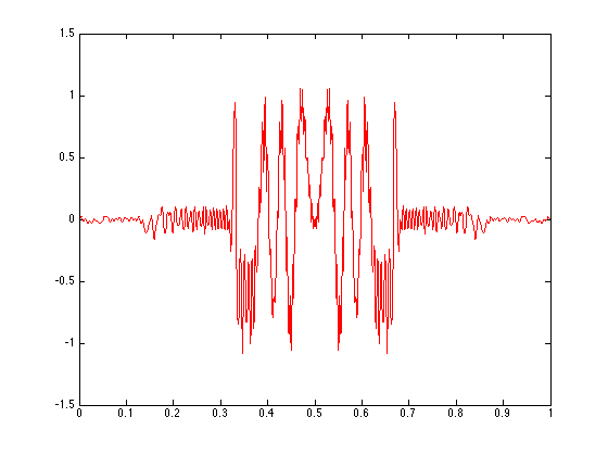
(a) Strang-Splitting solution

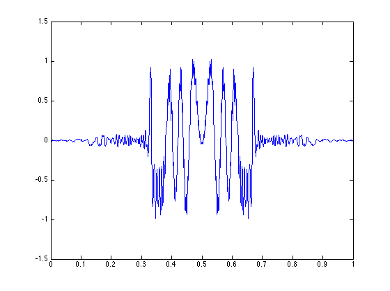
(b) Beam solution

(c) Comparison, center.

(d) Comparison, side.

Figure 1. Potential $V(x)=\cos(2\pi x)$. (A) The exact solution. (B) The beam solution. (C) and (D) Comparison of the exact and beam solution. “$\circ$”: the real solution; “$-$”: the beam solution.

We can push our analysis a little bit further. In Figure 2 our initial values are represented by the picture on the left-hand side, whereas on the right-hand side we show the same function multiplied by a narrower Gaussian. This provides an “almost” compactly supported function inside the interval $[0.25,0.75]$ where we have the potential well. In this case we obtain a $35\%$ drop on the relative error. The solution is shown in Figure 3, which contains a comparison of the exact and beam solution.

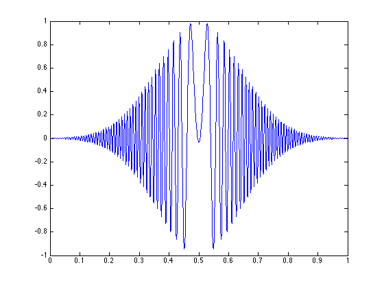
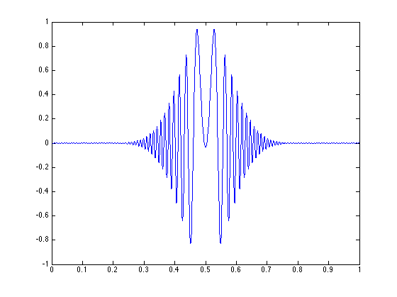
Figure 2. Initial values. The right one is numerically supported in $[0.25,0.75]$

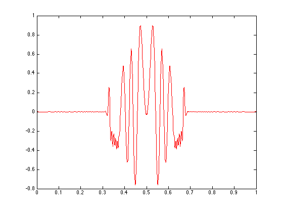
(a) Strang-Splitting solution

(b) Beam solution

(c) Comparison, center.

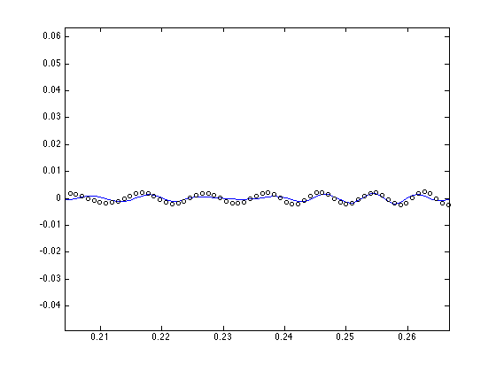
(d) Comparison, side.

Figure 3. Potential $V(x)=\cos(2\pi x)$, compactly supported initial values. (A) The exact solution. (B) The beam solution. (C) and (D) Comparison of the exact and beam solution. “$\circ$”: the real solution; “$-$”: the beam solution.

5.4.2. A potential Hill

Consider the initial value to be (64), we take the signal length to be $L=1024$ and the Plank constant $h=\frac{1}{256\pi}$, as above. We also set the same threshold $\eta=0.01$. We consider the potential $V(x)=\cos(2\pi(x+0.5))$, whose Hessian is non-positive for $x\in[0.25,0.75]$. This yields unacceptable numerical results for the standard algorithm, as shown in Figure 4.

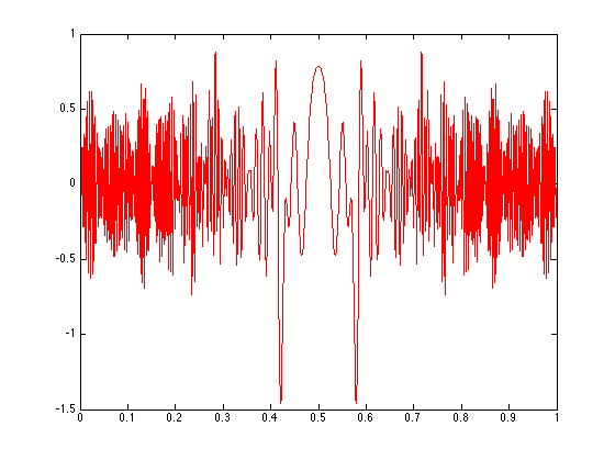
(a) Strang-Splitting solution

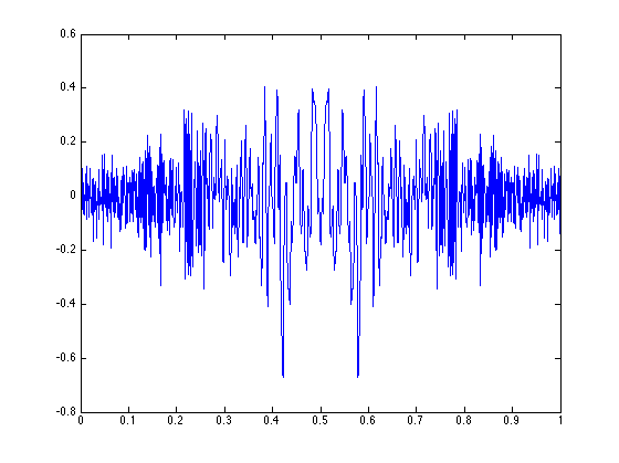
(b) Beam solution

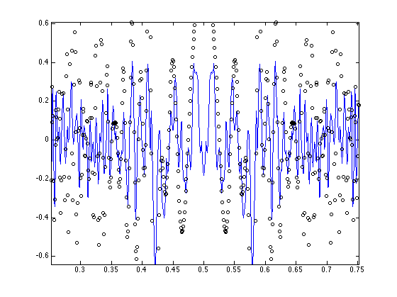
(c) Comparison, center.

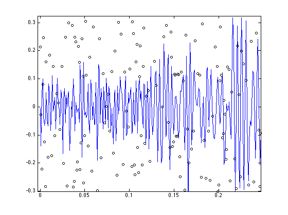
(d) Comparison, side.

Figure 4. Potential $V(x)=\cos(2\pi(x+0.5))$. (A) The exact solution. (B) The beam solution. (C) and (D) Comparison of the exact and beam solution. “$\circ$”: the real solution; “$-$”: the beam solution.

If we use the reinitialization algorithm, then our approximation improves a lot, see Figure 5. In this case we subdivide the time interval $[0,2]$ in eight uniform subintervals.

(a) Strang-Splitting solution

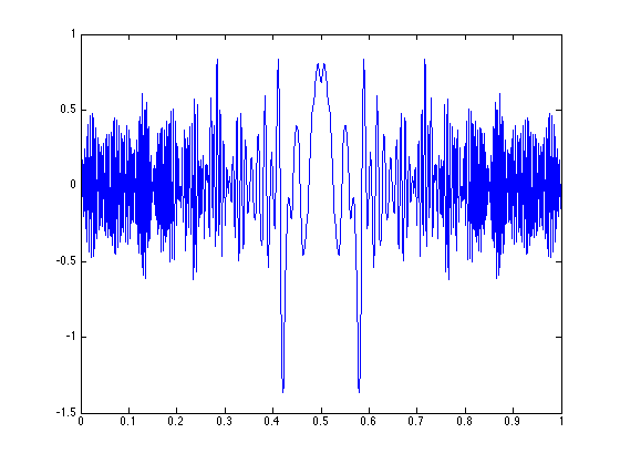
(b) Beam solution

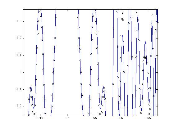
(c) Comparison, center.

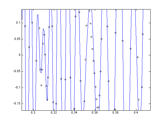
(d) Comparison, side.

Figure 5. Potential $V(x)=\cos(2\pi(x+0.5))$ with reinitialization. (A) The exact solution. (B) The beam solution. (C) and (D) Comparison of the exact and beam solution. “$\circ$”: the real solution; “$-$”: the beam solution.

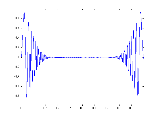
Figure 6. Shifted initial value

We can try to do as before and chose an initial value which is compactly supported in $[0,0.25]\cup[0.75,1]$, i.e. where the Hessian is non negative. The easiest way to do it is to shift the initial value used above by half the length of the signal, see Figure 6. Then, as shown in Figure 7, even without any reinitialization we get a perfect reconstruction, as expected. We notice that this is nothing but the first case shifted by half the wavelength.

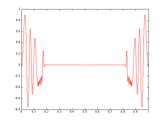
(a) Strang-Splitting solution

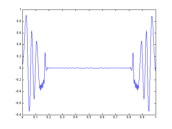
(b) Beam solution

Figure 7. Potential $V(x)=\cos(2\pi(x+0.5))$, compactly supported initial values.

5.4.3. A potential hill and well

Consider the initial value to be (64), we take the signal length to be $L=1024$ and the Plank constant $h=\frac{1}{256\pi}$, as above. We also set the same threshold $\eta=0.01$.
We take $V(x)=10+\sin(2\pi(x+0.5))$, whose Hessian is non-positive for $x\in[0,0.5]$. Once again, the numerical results without reinitialization are far from being consistent, see Figure 8.

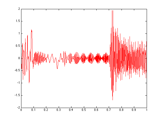
(a) Strang-Splitting solution

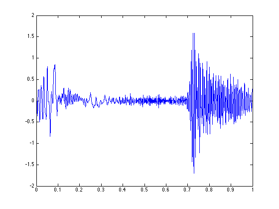
(b) Beam solution

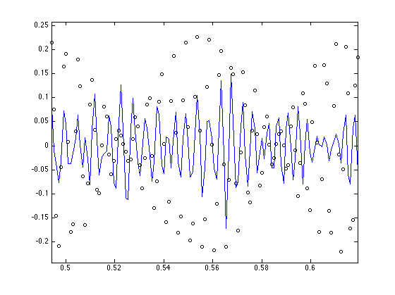
(c) Comparison, center.

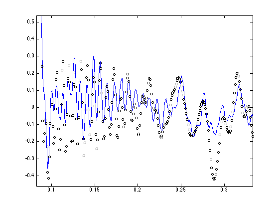
(d) Comparison, side.

Figure 8. Potential $V(x)=10+\sin(2\pi(x+0.5))$. (A) The exact solution. (B) The beam solution. (C) and (D) Comparison of the exact and beam solution. “$\circ$”: the real solution; “$-$”: the beam solution.

If we use the reinitialization, our results improve greatly as shown in Figure 9.

(a) Strang-Splitting solution

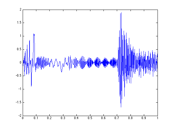
(b) Beam solution

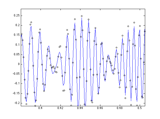
(c) Comparison, center.

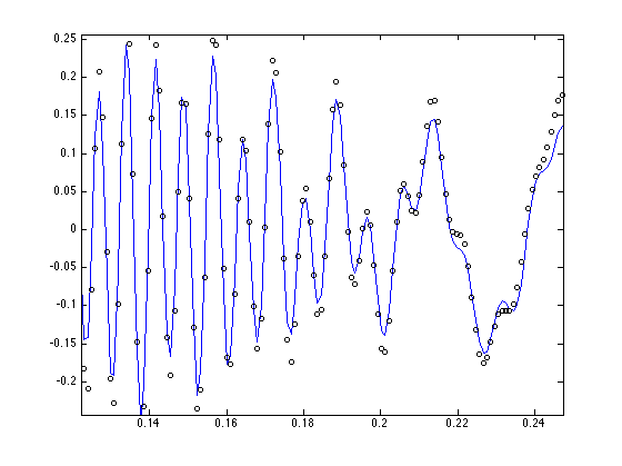
(d) Comparison, side.

Figure 9. Potential $V(x)=10+\sin(2\pi(x+0.5))$ with reinitialization. (A) The exact solution. (B) The beam solution. (C) and (D) Comparison of the exact and beam solution. “$\circ$”: the real solution; “$-$”: the beam solution.

We can try a similar trick as before and pick the usual compactly supported window shifted in the interval $[0.5,1]$, once again the results are very good, see Figure 10.

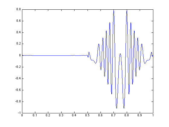
(a) Strang-Splitting solution

(b) Beam solution

Figure 10. Potential $V(x)=10+\sin(2\pi(x+0.5))$, compactly supported initial values.

5.5. Future Works

The LTFAT package provides a 2-dimensional discrete Gabor transform (dgt2), although the phaselock command is not yet available. Nevertheless, it seems possible to implement a multidimensional algorithm using the same approach. We plan to develop such a command and then investigate the two and three-dimensional cases.

References

- [1] G. Ascensi, H. G. Feichtinger, and N. Kaiblinger. Dilation of the Weyl symbol and Balian-Low theorem. Trans. Amer. Math. Soc., 366(7):3865–3880, 2014.
- [2] G. Bao, J. Lai, and J. Qian. Fast multiscale Gaussian beam methods for wave equations in bounded convex domains. J. Comput. Phys., 261:36–64, 2014.
- [3] G. Bao, J. Qian, L. Ying, and H. Zhang. A convergent multiscale Gaussian-beam parametrix for the wave equation. Comm. Partial Differential Equations, 38(1):92–134, 2013.
- [4] W. Bao, S. Jin, and P. A. Markowich. On time-splitting spectral approximations for the Schrödinger equation in the semiclassical regime. J. Comput. Phys., 175(2):487–524, 2002.
- [5] W. Bao, S. Jin, and P. A. Markowich. Numerical study of time-splitting spectral discretizations of nonlinear Schrödinger equations in the semiclassical regimes. SIAM J. Sci. Comput., 25(1):27–64, 2003.
- [6] M. Combescure and D. Robert. Coherent states and applications in mathematical physics. Theoretical and Mathematical Physics. Springer, Dordrecht, 2012.
- [7] M. Combescure and D. Robert. The quadratic hamiltonians. In Coherent States and Applications in Mathematical Physics, pages 59–85. Springer, 2012.
- [8] E. Cordero, K. Gröchenig, and F. Nicola. Approximation of Fourier integral operators by Gabor multipliers. J. Fourier Anal. Appl., 18(4):661–684, 2012.
- [9] E. Cordero, F. Nicola, and L. Rodino. Sparsity of Gabor representation of Schrödinger propagators. Applied and Computational Harmonic Analysis, 26(3):357–370, 2009.
- [10] E. Cordero, F. Nicola, and L. Rodino. Time-frequency analysis of Fourier integral operators. Commun. Pure Appl. Anal., 9(1):1–21, 2010.
- [11] E. Cordero, F. Nicola, and L. Rodino. Time-frequency analysis of Schrödinger propagators. In Evolution equations of hyperbolic and Schrödinger type, volume 301 of Progr. Math., pages 63–85. Birkhäuser/Springer Basel AG, Basel, 2012.
- [12] E. Cordero, F. Nicola, and L. Rodino. Wave packet analysis of Schrödinger equations in analytic function spaces. Submitted, arXiv:1310.5904.
- [13] E. Cordero, F. Nicola, and L. Rodino. Gabor representations of evolution operators. Trans. Amer. Math. Soc., to appear, arXiv:1209.0945.
- [14] E. Cordero, F. Nicola, and L. Rodino. Exponentially sparse representations of Fourier integral operators. Rev. Mat. Iberoam., to appear, arXiv:1301.1599.
- [15] E. Cordero, F. Nicola, and L. Rodino. Propagation of the Gabor wave front set for Schrödinger equations. Rev. in Mathematical Physics, to appear, arXiv:1309.0965.
- [16] E. Cordero, F. Nicola, and L. Rodino. Schrödinger equations with rough Hamiltonians. J. Discrete and Continuous Dynamical System - A, to appear, arXiv:1312.7791.
- [17] M. A. de Gosson. Symplectic methods in harmonic analysis and in mathematical physics, volume 7 of Pseudo-Differential Operators. Theory and Applications. Birkhäuser/Springer Basel AG, Basel, 2011.
- [18] M. A. de Gosson. Born-Jordan quantization and the equivalence of the Schrödinger and Heisenberg pictures, volume 44. 2014.
- [19] M. A. de Gosson. Hamiltonian deformations of gabor frames: First steps. Appl. Comput. Harmon. Anal., in press, 2014.
- [20] R. J. Duffin and A. C. Schaeffer. A class of nonharmonic fourier series. Trans. Amer. Math. Soc., 72:341–366, 1952.
- [21] H. G. Feichtinger and N. Kaiblinger. Varying the time-frequency lattice of Gabor frames. Trans. Amer. Math. Soc., 356(5):2001–2023 (electronic), 2004.
- [22] G. B. Folland. Harmonic analysis in phase space, volume 122 of Annals of Mathematics Studies. Princeton University Press, Princeton, NJ, 1989.
- [23] K. Gröchenig. Foundations of time-frequency analysis. Applied and Numerical Harmonic Analysis. Birkhäuser Boston, Inc., Boston, MA, 2001.
- [24] K. Gröchenig and Y. Lyubarskii. Gabor frames with Hermite functions. C. R. Math. Acad. Sci. Paris, 344(3):157–162, 2007.
- [25] K. Gröchenig, J. Ortega-Cerdà, and J. L. Romero. Deformation of Gabor systems. ArXiv e-prints, Nov. 2013.
- [26] K. Gröchenig and Z. Rzeszotnik. Banach algebras of pseudodifferential operators and their almost diagonalization. Ann. Inst. Fourier (Grenoble), 58(7):2279–2314, 2008.
- [27] V. Guillemin and S. Sternberg. Geometric asymptotics. American Mathematical Society, Providence, R.I., 1977. Mathematical Surveys, No. 14.
- [28] V. Guillemin and S. Sternberg. Symplectic techniques in physics. Cambridge University Press, Cambridge, second edition, 1990.
- [29] V. Guillemin and S. Sternberg. Semi-classical analysis. pages xxiv+446, 2013.
- [30] G. A. Hagedorn. Semiclassical quantum mechanics. I. The limit for coherent states. Comm. Math. Phys., 71(1):77–93, 1980.
- [31] G. A. Hagedorn. Semiclassical quantum mechanics. III. The large order asymptotics and more general states. Ann. Physics, 135(1):58–70, 1981.
- [32] J. R. Klauder and B.-S. Skagerstam, editors. Coherent states. World Scientific Publishing Co., Singapore, 1985. Applications in physics and mathematical physics.
- [33] D. Lugara, C. Letrou, A. Shlivinski, E. Heyman, and A. Boag. Frame-based gaussian beam summation method: Theory and applications. Radio Science, 38(2), 2003.
- [34] S. Luo. Deforming Gabor frames by quadratic Hamiltonians. Integral Transform. Spec. Funct., 9(1):69–74, 2000.
- [35] F. Nicola. Phase space analysis of semilinear parabolic equations. J. Funct. Anal., 267:727–743, 2014.
- [36] J. Qian and L. Ying. Fast Gaussian wavepacket transforms and Gaussian beams for the Schrödinger equation. J. Comput. Phys., 229(20):7848–7873, 2010.
- [37] J. Qian and L. Ying. Fast multiscale Gaussian wavepacket transforms and multiscale Gaussian beams for the wave equation. Multiscale Model. Simul., 8(5):1803–1837, 2010.
- [38] J. Ralston. Gaussian beams and the propagation of singularities. In Studies in partial differential equations, volume 23 of MAA Stud. Math., pages 206–248. Math. Assoc. America, Washington, DC, 1982.
- [39] D. Robert. Propagation of coherent states in quantum mechanics and applications. In Partial differential equations and applications, volume 15 of Sémin. Congr., pages 181–252. Soc. Math. France, Paris, 2007.
- [40] P. L. Sondergaard, P. C. Hansen, and O. Christensen. Finite discrete Gabor analysis. PhD thesis, Technical University of DenmarkDanmarks Tekniske Universitet, Department of Applied ChemistryInstitut for Anvendt Kemi, 2007.
- [41] P. L. Sondergaard, B. Torrésani, and P. Balazs. The linear time frequency analysis toolbox, 2012.
- [42] N. M. Tanushev, B. Engquist, and R. Tsai. Gaussian beam decomposition of high frequency wave fields. J. Comput. Phys., 228(23):8856–8871, 2009.
- [43] A. Waters. A parametrix construction for the wave equation with low regularity coefficients using a frame of Gaussians. Commun. Math. Sci., 9(1):225–254, 2011.
- [44] M. Zworski. Semiclassical analysis, volume 138 of Graduate Studies in Mathematics. American Mathematical Society, Providence, RI, 2012.