$p$th moment noise-to-state stability of stochastic differential equations with persistent noise

Abstract

This paper studies the stability properties of stochastic differential equations subject to persistent noise (including the case of additive noise), which is noise that is present even at the equilibria of the underlying differential equation and does not decay with time. The class of systems we consider exhibit disturbance attenuation outside a closed, not necessarily bounded, set. We identify conditions, based on the existence of Lyapunov functions, to establish the noise-to-state stability in probability and in pth moment of the system with respect to a closed set. As part of our analysis, we study the concept of two functions being proper with respect to each other formalized via pair of inequalities with comparison functions. We show that such inequalities define several equivalence relations for increasingly strong refinements on the comparison functions. We also provide a complete characterization of the properties that a pair of functions must satisfy to belong to the same equivalence class. This characterization allows us to provide checkable conditions to determine whether a function satisfies the requirements to be a strong NSS-Lyapunov function in probability or a $p$th moment NSS-Lyapunov function. Several examples illustrate our results.

1 Introduction

Stochastic differential equations (SDEs) go beyond ordinary differential equations (ODEs) to deal with systems subject to stochastic perturbations of a particular type, known as white noise. Applications are numerous and include option pricing in the stock market, networked systems with noisy communication channels, and, in general, scenarios whose complexity cannot be captured by deterministic models. In this paper, we study SDEs subject to persistent noise (including the case of additive noise), i.e., systems for which the noise is present even at the equilibria of the underlying ODE and does not decay with time. Such scenarios arise, for instance, in control-affine systems when the input is corrupted by persistent noise. For these systems, the presence of persistent noise makes it impossible to establish in general a stochastic notion of asymptotic stability for the (possibly unbounded) set of equilibria of the underlying ODE. Our aim here is to develop notions and tools to study the stability properties of these systems and provide probabilistic guarantees on the size of the state of the system.

Literature review: In general, it is not possible to obtain explicit descriptions of the solutions of SDEs. Fortunately, the Lyapunov techniques used to study the qualitative behavior of ODEs [6, 10] can be adapted to study the stability properties of SDEs as well [7, 27, 13]. Depending on the notion of stochastic convergence used, there are several types of stability results in SDEs. These include stochastic stability (or stability in probability), stochastic asymptotic stability, almost sure exponential stability, and pth moment asymptotic stability, see e.g., [27, 13, 14, 26]. However, these notions are not appropriate in the presence of persistent noise because they require the effect of the noise on the set of equilibria to either vanish or decay with time. To deal with persistent noise, as well as other system properties like delays, a concept of ultimate boundedness is required that generalizes the notion of convergence. As an example, for stochastic delay differential equations, [28] considers a notion of ultimate bound in $p$th moment [21] and employs Lyapunov techniques to establish it. More generally, for mean-square random dynamical systems, the concept of forward attractor [9] describes a notion of convergence to a dynamic neighborhood and employs contraction analysis to establish it. Similar notions of ultimate boundedness for the state of a system, now in terms of the size of the disturbance, are also used for differential equations, and many of these notions are inspired by dissipativity properties of the system that are captured via dissipation inequalities of a suitable Lyapunov function: such inequalities encode the fact that the Lyapunov function decreases along the trajectories of the system as long as the state is “big enough” with regards to the disturbance. As an example, the concept of input-to-state stability (ISS) goes hand in hand with the concept of ISS-Lyapunov function, since the existence of the second implies the former (and, in many cases, a converse result is also true [24]). Along these lines, the notion of practical stochastic input-to-state stability (SISS) in [12, 29] generalizes the concept of ISS to SDEs where the disturbance or input affects both the deterministic term of the dynamics and the diffusion term modeling the role of the noise. Under this notion, the state bound is guaranteed in probability, and also depends, as in the case of ISS, on a decaying effect of the initial condition plus an increasing function of the sum of the size of the input and a positive constant related to the persistent noise. For systems where the input modulates the covariance of the noise, SISS corresponds to noise-to-state-stability (NSS) [3], which guarantees, in probability, an ultimate bound for the state that depends on the magnitude of the noise covariance. That is, the noise in this case plays the main role, since the covariance can be modulated arbitrarily and can be unknown. This is the appropriate notion of stability for the class of SDEs with persistent noise considered in this paper, which are nonlinear systems affine in the input, where the input corresponds to white noise with locally bounded covariance. Such systems cannot be studied under the ISS umbrella, because the stochastic integral against Brownian motion has infinite variation, whereas the integral of a legitimate input for ISS must have finite variation.

Statement of contributions: The contributions of this paper are twofold. Our first contribution concerns the noise-to-state stability of systems described by SDEs with persistent noise. We generalize the notion of noise-dissipative Lyapunov function, which is a positive semidefinite function that satisfies a dissipation inequality that can be nonexponential (by this we mean that the inequality admits a convex $\mathcal{K}_{\infty}$ gain instead of the linear gain characteristic of exponential dissipativity). We also introduce the concept of $p$thNSS-Lyapunov function with respect to a closed set, which is a noise-dissipative Lyapunov function that in addition is proper with respect to the set with a convex lower-bound gain function. Using this framework, we show that noise-dissipative Lyapunov functions have NSS dynamics and we characterize the overshoot gain. More importantly, we show that the existence of a pthNSS-Lyapunov function with respect to a closed set implies that the system is NSS in pth moment with respect to the set. Our second contribution is driven by the aim of providing alternative, structured ways to check the hypotheses of the above results. We introduce the notion of two functions being proper with respect to each other as a generalization of the notion of properness with respect to a set. We then develop a methodology to verify whether two functions are proper with respect to each other by analyzing the associated pair of inequalities with increasingly strong refinements that involve the classes $\mathcal{K}$, $\mathcal{K}_{\infty}$, and $\mathcal{K}_{\infty}$ plus a convexity property. We show that these refinements define equivalence relations between pairs of functions, thereby producing nested partitions on the space of functions. This provides a useful way to deal with these inequalities because the construction of the gains is explicit when the transitivity property is exploited. This formalism motivates our characterization of positive semidefinite functions that are proper, in the various refinements, with respect to the Euclidean distance to their nullset. This characterization is technically challenging because we allow the set to be noncompact, and thus the pre-comparison functions can be discontinuous. We devote special attention to the case when the set is a subspace and examine the connection with seminorms. Finally, we show how this framework allows us to develop an alternative formulation of our stability results.

Organization: The paper is organized as follows. Section 2 introduces preliminaries on seminorms, comparison functions, and SDEs. Section 3 presents the NSS stability results and Section 4 develops the methodology to help verify their hypotheses. Finally, Section 5 discusses our conclusions and ideas for future work.

2 Preliminary notions

This section reviews some notions on comparison functions and stochastic differential equations that are used throughout the paper.

2.1 Notational conventions

Let ${\mathbb{R}}$ and ${\mathbb{R}}_{\geq 0}$ be the sets of real and nonnegative real numbers, respectively. We denote by ${\mathbb{R}}^{n}$ the $n$-dimensional Euclidean space. A subspace $\mathcal{U}\subseteq{\mathbb{R}}^{n}$ is a subset which is also a vector space. Given a matrix $A\in\mathbb{R}^{m\times n}$, its nullspace $\operatorname{\mathcal{N}}(A)\triangleq\{x\in{\mathbb{R}}^{n}:Ax=0\}$ is a subspace. Given $\mathcal{D}\subseteq{\mathbb{R}}^{n}$, we denote by $\mathcal{C}(\mathcal{D}\,;{\mathbb{R}}_{{\text{\scalebox{0.7}{$\geq 0$}}}})$ and $\mathcal{C}^{2}(\mathcal{D}\,;{\mathbb{R}}_{{\text{\scalebox{0.7}{$\geq 0$}}}})$ the set of positive semidefinite functions defined on $\mathcal{D}$ that are continuous and continuously twice differentiable (if $\mathcal{D}$ is open), respectively. Given $\mathrm{V}\in\mathcal{C}^{2}({\mathbb{R}}^{n};{\mathbb{R}}_{{\text{\scalebox{0.7}{$\geq 0$}}}})$, we denote its gradient by $\nabla\mathrm{V}$ and its Hessian by $\nabla^{2}\mathrm{V}$. A seminorm is a function $S:{\mathbb{R}}^{n}\to{\mathbb{R}}$ that is positively homogeneous, i.e., $S(\lambda x)=|\lambda|S(x)$ for any $\lambda\in{\mathbb{R}}$, and satisfies the triangular inequality, i.e., $S(x+y)\leq S(x)+S(y)$ for any $x,y\in{\mathbb{R}}^{n}$. From these properties it can be deduced that $S\in\mathcal{C}({\mathbb{R}}^{n};{\mathbb{R}}_{{\text{\scalebox{0.7}{$\geq 0$}}}})$ and its nullset is always a subspace. If, moreover, the function $S$ is positive definite, i.e., $S(x)=0$ implies $x=0$, then $S$ is a norm. The Euclidean norm of $x\in{\mathbb{R}}^{n}$ is denoted by $\|x\|_{\text{\scalebox{1.0}{$2$}}}$, and the Frobenius norm of the matrix $A\in\mathbb{R}^{m\times n}$ is $|A|_{\text{\scalebox{0.8}{$\mathcal{F}$}}}\triangleq\sqrt{\operatorname{trace}{(A^{\text{\scalebox{0.8}{$T$}}}A)}}=\sqrt{\operatorname{trace}{(AA^{\text{\scalebox{0.8}{$T$}}})}}$. For any matrix $A\in\mathbb{R}^{m\times n}$, the function $\|x\|_{\text{\scalebox{1.0}{$A$}}}\triangleq\|Ax\|_{\text{\scalebox{1.0}{$2$}}}$ is a seminorm and can be viewed as a distance to $\operatorname{\mathcal{N}}(A)$. For a symmetric positive semidefinite real matrix $A\in{\mathbb{R}^{n\times n}}$, we order its eigenvalues as $\operatorname{\lambda_{\text{max}}}(A)\triangleq\lambda_{1}(A)\geq\dots\geq\lambda_{n}(A)\triangleq\operatorname{\lambda_{\text{min}}}(A)$, so if the dimension of $\operatorname{\mathcal{N}}(A)$ verifies $\dim(\operatorname{\mathcal{N}}(A))=k\leq n$, then $\lambda_{n-k}(A)$ is the minimum nonzero eigenvalue of $A$. The Euclidean distance from $x$ to a set $\mathcal{U}\subseteq{\mathbb{R}}^{n}$ is defined by $|x|_{\text{\scalebox{0.7}{$\mathcal{U}$}}}\triangleq\inf\{\|x-u\|_{\text{\scalebox{1.0}{$2$}}}\,:\,u\in\mathcal{U}\}$. The function $|.|_{\text{\scalebox{0.7}{$\mathcal{U}$}}}$ is continuous when $\mathcal{U}$ is closed. Given $f,g:{\mathbb{R}}_{\geq 0}\rightarrow{\mathbb{R}}_{\geq 0}$, we say that $f(s)$ is in $\mathcal{O}(g(s))$ as $s\to\infty$ if there exist constants $\kappa,s_{0}>0$ such that $f(s)<\kappa g(s)$ for all $s>s_{0}$.

2.2 Comparison, convex, and concave functions

Here we introduce some classes of comparison functions following [6] that are useful in our technical treatment. A continuous function $\alpha:[0,b)\to{\mathbb{R}}_{\geq 0}$, for $b>0$ or $b=\infty$, is class $\mathcal{K}$ if $\alpha(0)=0$ and is strictly increasing. A function $\alpha:{\mathbb{R}}_{\geq 0}\rightarrow{\mathbb{R}}_{\geq 0}$ is class $\mathcal{K}_{\infty}$ if $\alpha\in\mathcal{K}$ and is unbounded. A continuous function $\mu:{\mathbb{R}}_{\geq 0}\times{\mathbb{R}}_{\geq 0}\rightarrow{\mathbb{R}}_{\geq 0}$ is class $\mathcal{KL}$ if, for each fixed $s\geq 0$, the function $r\mapsto\mu(r,s)$ is class $\mathcal{K}$, and, for each fixed $r\geq 0$, the function $s\mapsto\mu(r,s)$ is decreasing and $\lim_{s\to\infty}\mu(r,s)=0$. If $\alpha_{1}$, $\alpha_{2}$ are class $\mathcal{K}$ and the domain of $\alpha_{1}$ contains the range of $\alpha_{2}$, then their composition $\alpha_{1}\circ\alpha_{2}$ is class $\mathcal{K}$ too. If $\alpha_{3}$, $\alpha_{4}$ are class $\mathcal{K}_{\infty}$, then both the inverse function $\alpha_{3}^{-1}$ and their composition $\alpha_{3}\circ\alpha_{4}$ are class $\mathcal{K}_{\infty}$. In our technical treatment, it is sometimes convenient to require comparison functions to satisfy additional convexity properties. A real-valued function $f$ defined in a convex set $X$ in a vector space is convex if $f(\lambda x+(1-\lambda)y)\leq\lambda f(x)+(1-\lambda)f(y)$ for each $x,y\in X$ and any $\lambda\in[0,1]$, and is concave if $-f$ is convex. By [2, Ex. 3.3], if $f:[a,b]\to[f(a),f(b)]$ is a strictly increasing convex (respectively, concave) function, then the inverse function $f^{-1}:[f(a),f(b)]\to[a,b]$ is strictly increasing and concave (respectively, convex). Also, following [2, Section 3], if $f,g:{\mathbb{R}}\to{\mathbb{R}}$ are convex (respectively, concave) and $f$ is nondecreasing, then the composition $f\circ g$ is also convex (respectively, concave).

2.3 Brownian motion

We review some basic facts on probability and introduce the notion of Brownian motion following [14]. Throughout the paper, we assume that $(\Omega,\mathcal{F},\{\mathcal{F}_{t}\}_{t\geq 0},\mathbb{P})$ is a complete probability space, where $\mathbb{P}$ is a probability measure defined on the $\sigma$-algebra $\mathcal{F}$, which contains all the subsets of $\Omega$ of probability $0$. The filtration $\{\mathcal{F}_{t}\}_{t\geq 0}$ is a family of sub-$\sigma$-algebras of $\mathcal{F}$ satisfying $\mathcal{F}_{t}\subseteq\mathcal{F}_{s}\subseteq\mathcal{F}$ for any $0\leq t<s<\infty$; we assume it is right continuous, i.e., $\mathcal{F}_{t}=\cap_{s>t}\mathcal{F}_{s}$ for any $t\geq 0$, and $\mathcal{F}_{0}$ contains all the subsets of $\Omega$ of probability $0$. The Borel $\sigma$-algebra in ${\mathbb{R}}^{n}$, denoted by $\mathcal{B}^{n}$, or in $[t_{0},\infty)$, denoted by $\mathcal{B}([t_{0},\infty))$, are the smallest $\sigma$-algebras that contain all the open sets in ${\mathbb{R}}^{n}$ or $[t_{0},\infty)$, respectively. A function $X:\Omega\to{\mathbb{R}}^{n}$ is $\mathcal{F}$-measurable if the set $\{\omega\in\Omega:X(\omega)\in A\}$ belongs to $\mathcal{F}$ for any $A\in\mathcal{B}^{n}$. We call such function a ($\mathcal{F}$-measurable) ${\mathbb{R}}^{n}$-valued random variable. If $X$ is a real-valued random variable that is integrable with respect to $\mathbb{P}$, its expectation is $\mathbb{E}[X]=\int_{\Omega}X(\omega)\mathrm{d}\mathbb{P}(\omega)$. A function $f:\Omega\times[t_{0},\infty)\to{\mathbb{R}}^{n}$ is $\mathcal{F}\times\mathcal{B}$-measurable (or just measurable) if the set $\{(\omega,t)\in\Omega\times[t_{0},\infty):f(\omega,t)\in A\}$ belongs to $\mathcal{F}\times\mathcal{B}([t_{0},\infty))$ for any $A\in\mathcal{B}^{n}$. We call such function an $\{\mathcal{F}_{t}\}$-adapted process if $f(.,t):\Omega\rightarrow{\mathbb{R}}^{n}$ is $\mathcal{F}_{t}$-measurable for every $t\geq t_{0}$. At times, we omit the dependence on “$\omega$”, in the sense that we refer to the indexed family of random variables, and refer to the random process $f=\{f(t)\}_{t\geq t_{0}}$. We define $\mathcal{L}^{1}([t_{0},\infty);{\mathbb{R}}^{n})$ as the set of all ${\mathbb{R}}^{n}$-valued measurable $\{\mathcal{F}_{t}\}$-adapted processes $f$ such that $\mathbb{P}(\{\omega\in\Omega\,:\,\int_{t_{0}}^{T}\|f(\omega,s)\|_{\text{\scalebox{1.0}{$2$}}}\,\mathrm{d}s<\infty\})=1$ for every $T>t_{0}$. Similarly, $\mathcal{L}^{2}([t_{0},\infty);{\mathbb{R}}^{n\times m})$ denotes the set of all ${\mathbb{R}^{n\times m}}$-matrix-valued measurable $\{\mathcal{F}_{t}\}$-adapted processes $G$ such that $\mathbb{P}(\{\omega\in\Omega\,:\,\int_{t_{0}}^{T}|G(\omega,s)|_{\text{\scalebox{0.8}{$\mathcal{F}$}}}^{2}\,\mathrm{d}s<\infty\})=1$ for every $T>t_{0}$.

A one-dimensional Brownian motion $\mathrm{B}:\Omega\times[t_{0},\infty)\rightarrow{\mathbb{R}}$ defined in the probability space $(\Omega,\mathcal{F},\{\mathcal{F}_{t}\}_{t\geq 0},\mathbb{P})$ is an $\{\mathcal{F}_{t}\}$-adapted process such that

• $\mathbb{P}(\{\omega\in\Omega\,:\,\mathrm{B}(\omega,t_{0})=0\})=1$;

• the mapping $\mathrm{B}(\omega,.):[t_{0},\infty)\rightarrow{\mathbb{R}}$, called sample path, is continuous also with probability $1$;

• the increment $\mathrm{B}(.,t)-\mathrm{B}(.,s):\Omega\to{\mathbb{R}}$ is independent of $\mathcal{F}_{s}$ for $t_{0}\leq s<t<\infty$ (i.e., if $S_{b}\triangleq\{\omega\in\Omega:\mathrm{B}(\omega,t)-\mathrm{B}(\omega,s)\in(-\infty,b)\}$, for $b\in{\mathbb{R}}$, then $\mathbb{P}(A\cap S_{b})=\mathbb{P}(A)\mathbb{P}(S_{b})$ for all $A\in\mathcal{F}_{s}$ and all $b\in{\mathbb{R}}$). In addition, this increment is normally distributed with zero mean and variance $t-s$.

An $m$-dimensional Brownian motion $\mathrm{B}:\Omega\times[t_{0},\infty)\rightarrow{\mathbb{R}}^{m}$ is given by $\mathrm{B}(\omega,t)=[\mathrm{B}_{1}(\omega,t),\dots,\mathrm{B}_{m}(\omega,t)]^{\text{\scalebox{0.8}{$T$}}}$, where each $\mathrm{B}_{i}$ is a one-dimensional Brownian motion and, for each $t\geq t_{0}$, the random variables $\mathrm{B}_{1}(t),...,\mathrm{B}_{m}(t)$ are independent.

2.4 Stochastic differential equations

Here we review some basic notions on stochastic differential equations (SDEs) following [14]; other useful references are [7, 18, 17]. Consider the $n$-dimensional SDE

(1) $$\mathrm{d}x(\omega,t)=f\big{(}x(\omega,t),t\big{)}\mathrm{d}t+G\big{(}x(\omega,t),t\big{)}\Sigma(t)\,\mathrm{dB}(\omega,t),$$

where $x(\omega,t)\in{\mathbb{R}}^{n}$ is a realization at time $t$ of the random variable $x(.,t):\Omega\rightarrow{\mathbb{R}}^{n}$, for $t\in[t_{0},\infty)$. The initial condition is given by $x(\omega,t_{0})=x_{0}$ with probability $1$ for some $x_{0}\in{\mathbb{R}}^{n}$. The functions $f:{\mathbb{R}}^{n}\times[t_{0},\infty)\rightarrow{\mathbb{R}}^{n}$, $G:{\mathbb{R}}^{n}\times[t_{0},\infty)\to\mathbb{R}^{n\times q}$, and $\Sigma:[t_{0},\infty)\rightarrow\mathbb{R}^{q\times m}$ are measurable. The functions $f$ and $G$ are regarded as a model for the architecture of the system and, instead, $\Sigma$ is part of the model for the stochastic disturbance; at any given time $\Sigma$ determines a linear transformation of the $m$-dimensional Brownian motion $\{\mathrm{B}(t)\}_{t\geq t_{0}}$, so that at time $t\geq t_{0}$ the input to the system is the process $\{\Sigma(t)\mathrm{B}(t)\}_{t\geq t_{0}}$, with covariance $\int_{t_{0}}^{t}\Sigma(t)\Sigma(t)^{\text{\scalebox{0.8}{$T$}}}\mathrm{d}s$. The distinction between the roles of $G$ and $\Sigma$ is irrelevant for the SDE; both together determine the effect of the Brownian motion. The integral form of (1) is given by

$$x(\omega,t)=x_{0}+\int_{t_{0}}^{t}f\big{(}x(\omega,s),s\big{)}\mathrm{d}s+\int_{t_{0}}^{t}G\big{(}x(\omega,s),s\big{)}\Sigma(s)\,\mathrm{dB}(\omega,s),$$

where the second integral is an stochastic integral [14, p. 18]. A ${\mathbb{R}}^{n}$-valued random process $\{x(t)\}_{t\geq t_{0}}$ is a solution of (1) with initial value $x_{0}$ if

1. is continuous with probability $1$, $\{\mathcal{F}_{t}\}$-adapted, and satisfies $x(\omega,t_{0})=x_{0}$ with probability $1$,

2. the processes $\{f(x(t),t)\}_{t\geq t_{0}}$ and $\{G(x(t),t)\}_{t\geq t_{0}}$ belong to $\mathcal{L}^{1}([t_{0},\infty);{\mathbb{R}}^{n})$ and $\mathcal{L}^{2}([t_{0},\infty);{\mathbb{R}}^{n\times m})$ respectively, and

3. equation (1) holds for every $t\geq t_{0}$ with probability $1$.

A solution $\{x(t)\}_{t\geq t_{0}}$ of (1) is unique if any other solution $\{\bar{x}(t)\}_{t\geq t_{0}}$ with $\bar{x}(t_{0})=x_{0}$ differs from it only in a set of probability $0$, that is, $\mathbb{P}(\big{\{}x(t)=\bar{x}(t)$  $\forall\,t\geq t_{0}\big{\}})=1$.

We make the following assumptions on the objects defining (1) to guarantee existence and uniqueness of solutions.

Assumption 1.

We assume $\Sigma$ is essentially locally bounded. Furthermore, for any $T>t_{0}$ and $n\geq 1$, we assume there exists $K_{T,n}>0$ such that, for almost every $t\in[t_{0},T]$ and all $x,y\in{\mathbb{R}}^{n}$ with $\max\big{\{}\|x\|_{\text{\scalebox{1.0}{$2$}}},\|y\|_{\text{\scalebox{1.0}{$2$}}}\big{\}}\leq n$,

$$\max \big{\{}\,\|f(x,t)-f(y,t)\|_{\text{\scalebox{1.0}{$2$}}}^{2}\,,\,|G(x,t)-G(y,t)|_{\text{\scalebox{0.8}{$\mathcal{F}$}}}^{2}\,\big{\}}\leq K_{T,n}\|x-y\|_{\text{\scalebox{1.0}{$2$}}}^{2}.$$

Finally, we assume that for any $T>t_{0}$, there exists $K_{T}>0$ such that, for almost every $t\in[t_{0},T]$ and all $x\in{\mathbb{R}}^{n}$, $x^{\text{\scalebox{0.8}{$T$}}}f(x,t)+\tfrac{1}{2}|G(x,t)|_{\text{\scalebox{0.8}{$\mathcal{F}$}}}^{2}\leq K_{T}(1+\|x\|_{\text{\scalebox{1.0}{$2$}}}^{2})$.

According to [14, Th. 3.6, p. 58], Assumption 1 is sufficient to guarantee global existence and uniqueness of solutions of (1) for each initial condition $x_{0}\in{\mathbb{R}}^{n}$.

We conclude this section by presenting a useful operator in the stability analysis of SDEs. Given a function $\mathrm{V}\in\mathcal{C}^{2}({\mathbb{R}}^{n};{\mathbb{R}}_{{\text{\scalebox{0.7}{$\geq 0$}}}})$, we define the generator of (1) acting on the function $\mathrm{V}$ as the mapping $\mathcal{L}[\mathrm{V}]:{\mathbb{R}}^{n}\times[t_{0},\infty)\rightarrow{\mathbb{R}}$ given by

(2) $$\mathcal{L}[\mathrm{V}](x,t)\triangleq\nabla\mathrm{V}(x)^{\text{\scalebox{0.8}{$T$}}}f(x,t)+\tfrac{1}{2}\operatorname{trace}\Big{(}\Sigma(t)^{\text{\scalebox{0.8}{$T$}}}G(x,t)^{\text{\scalebox{0.8}{$T$}}}\nabla^{2}\mathrm{V}(x)G(x,t)\Sigma(t)\Big{)}.$$

It can be shown that $\mathcal{L}[\mathrm{V}](x,t)$ gives the expected rate of change of $\mathrm{V}$ along a solution of (1) that passes through the point $x$ at time $t$, so it is a generalization of the Lie derivative. According to [14, Th. 6.4, p. 36], if we evaluate $\mathrm{V}$ along the solution $\{x(t)\}_{t\geq t_{0}}$ of (1), then the process $\{\mathrm{V}(x(t))\}_{t\geq t_{0}}$ satisfies the new SDE

(3) $$\mathrm{V}(x(t)) =\mathrm{V}(x_{0})+\int_{t_{0}}^{t}\mathcal{L}[\mathrm{V}](x(s),s)\mathrm{d}s+\int_{t_{0}}^{t}\nabla\mathrm{V}(x(s))^{\text{\scalebox{0.8}{$T$}}}G(x(s),s)\Sigma(s)\mathrm{dB}(s).$$

Equation (3) is known as Itô’s formula and corresponds to the stochastic version of the chain rule.

3 Noise-to-state stability via noise-dissipative Lyapunov functions

In this section, we study the stability of stochastic differential equations subject to persistent noise. Our first step is the introduction of a novel notion of stability. This captures the behavior of the $p$th moment of the distance (of the state) to a given closed set, as a function of two objects: the initial condition and the maximum size of the covariance. After this, our next step is to derive several Lyapunov-type stability results that help determine whether a stochastic differential equation enjoys these stability properties. The following definition generalizes the concept of noise-to-state stability given in [3].

Definition 2.

(Noise-to-state stability with respect to a set). The system (1) is noise-to-state stable (NSS) in probability with respect to the set $\mathcal{U}\subseteq{\mathbb{R}}^{n}$ if for any $\epsilon>0$ there exist $\mu\in\mathcal{KL}$ and $\theta\in\mathcal{K}$ (that might depend on $\epsilon$), such that

(4) $$\mathbb{P}\Big{\{}\,|x(t)|_{\text{\scalebox{0.7}{$\mathcal{U}$}}}^{p}>\mu\big{(}|x_{0}|_{\text{\scalebox{0.7}{$\mathcal{U}$}}},t-t_{0}\big{)}+\theta\Big{(}\operatorname*{ess\,sup}_{t_{0}\leq s\leq t}|\Sigma(s)|_{\text{\scalebox{0.8}{$\mathcal{F}$}}}\Big{)}\,\Big{\}}\leq\epsilon,$$

for all $t\geq t_{0}$ and any $x_{0}\in{\mathbb{R}}^{n}$. And the system (1) is $p$th moment noise-to-state stable ($p$thNSS) with respect to $\mathcal{U}$ if there exist $\mu\in\mathcal{KL}$ and $\theta\in\mathcal{K}$, such that

(5) $$\mathbb{E}\big{[}|x(t)|_{\text{\scalebox{0.7}{$\mathcal{U}$}}}^{p}\big{]} \leq\mu\big{(}|x_{0}|_{\text{\scalebox{0.7}{$\mathcal{U}$}}},t-t_{0}\big{)}+\theta\Big{(}\operatorname*{ess\,sup}_{t_{0}\leq s\leq t}|\Sigma(s)|_{\text{\scalebox{0.8}{$\mathcal{F}$}}}\Big{)},$$

for all $t\geq t_{0}$ and any $x_{0}\in{\mathbb{R}}^{n}$. The gain functions $\mu$ and $\theta$ are the overshoot gain and the noise gain, respectively.

The quantity $|\Sigma(t)|_{\text{\scalebox{0.8}{$\mathcal{F}$}}}=\sqrt{\operatorname{trace}\big{(}\Sigma(t)\Sigma(t)^{\text{\scalebox{0.8}{$T$}}}\big{)}}$ is a measure of the size of the noise because it is related to the infinitesimal covariance $\Sigma(t)\Sigma(t)^{\text{\scalebox{0.8}{$T$}}}$. The choice of the $p$th power is irrelevant in the statement in probability since one could take any $\mathcal{K}_{\infty}$ function evaluated at $|x(t)|_{\text{\scalebox{0.7}{$\mathcal{U}$}}}$. However, this would make a difference in the statement in expectation. (Also, we use the same power for convenience.) When the set $\mathcal{U}$ is a subspace, we can substitute $|.|_{\text{\scalebox{0.7}{$\mathcal{U}$}}}$ by $\|.\|_{\text{\scalebox{1.0}{$A$}}}$, for some matrix $A\in\mathbb{R}^{m\times n}$ with $\operatorname{\mathcal{N}}(A)=\mathcal{U}$. In such a case, the definition above does not depend on the choice of the matrix $A$.

Remark 3.

(NSS is not a particular case of ISS). The concept of NSS is not a particular case of input-to-state stability (ISS) [23] for systems that are affine in the input, namely,

$$\dot{y}=f(y,t)+G(y,t)u(t)\;\>\Leftrightarrow\;\>y(t)=y(t_{0})+\int_{t_{0}}^{t}f(y(s),s)\,\mathrm{d}s+\int_{t_{0}}^{t}G(y(s),s)u(s)\,\mathrm{d}s,$$

where $u:[t_{0},\infty)\rightarrow{\mathbb{R}}^{q}$ is measurable and essentially locally bounded [22, Sec. C.2]. The reason is the following: the components of the vector-valued function $\int_{t_{0}}^{t}G(y(s),s)u(s)\,\mathrm{d}s$ are differentiable almost everywhere by the Lebesgue fundamental theorem of calculus [16, p. 289], and thus absolutely continuous [16, p. 292] and with bounded variation [16, Prop. 8.5]. On the other hand, at any time previous to $t_{k}(t)\triangleq\min\{t,\inf{\{s\geq t_{0}\,:\,\|x(s)\|_{\text{\scalebox{1.0}{$2$}}}\geq k\}}\}$, the driving disturbance of (1) is the vector-valued function $\int_{t_{0}}^{t_{k}(t)}G(x(s),s)\Sigma(s)\mathrm{dB}(s)$, whose $i$th component has quadratic variation [14, Th. 5.14, p. 25] equal to

$$\int_{t_{0}}^{t_{k}(t)}\sum\limits_{j=1}^{m}|\sum\limits_{l=1}^{q}G(x(s),s)_{il}\Sigma(s)_{lj}|^{2}\mathrm{d}s>0.$$

Since a continuous process that has positive quadratic variation must have infinite variation [8, Th. 1.10], we conclude that the driving disturbance in this case is not allowed in the ISS framework. $\bullet$

Our first goal now is to provide tools to establish whether a stochastic differential equation enjoys the noise-to-state stability properties given in Definition 2. To achieve this, we look at the dissipativity properties of a special kind of energy functions along the solutions of (1).

Definition 4.

(Noise-dissipative Lyapunov function). A function $\mathrm{V}\in\mathcal{C}^{2}({\mathbb{R}}^{n};{\mathbb{R}}_{{\text{\scalebox{0.7}{$\geq 0$}}}})$ is a noise-dissipative Lyapunov function for (1) if there exist $\mathrm{W}\in\mathcal{C}({\mathbb{R}}^{n};{\mathbb{R}}_{{\text{\scalebox{0.7}{$\geq 0$}}}})$, $\sigma\in\mathcal{K}$, and concave $\eta\in\mathcal{K}_{\infty}$ such that

(6) $$\mathrm{V}(x)\leq\eta(\mathrm{W}(x)),$$

for all $x\in{\mathbb{R}}^{n}$, and the following dissipation inequality holds:

(7) $$\mathcal{L}[\mathrm{V}](x,t)\leq-\mathrm{W}(x)+\sigma\big{(}|\Sigma(t)|_{\text{\scalebox{0.8}{$\mathcal{F}$}}}\big{)},$$

for all $(x,t)\in{\mathbb{R}}^{n}\times[t_{0},\infty)$.

Remark 5.

(Itô formula and exponential dissipativity). Interestingly, the conditions (6) and (7) are equivalent to

(8) $$\mathcal{L}[\mathrm{V}](x,t)\leq-\eta^{-1}(\mathrm{V}(x))+\sigma\big{(}|\Sigma(t)|_{\text{\scalebox{0.8}{$\mathcal{F}$}}}\big{)},$$

for all $x\in{\mathbb{R}}^{n}$, where $\eta^{-1}\in\mathcal{K}_{\infty}$ is convex. Note that, since $\mathcal{L}[\mathrm{V}]$ is not the Lie derivative of $\mathrm{V}$ (as it contains the Hessian of $\mathrm{V}$), one cannot directly deduce from (8) the existence of a continuously twice differentiable function $\tilde{\mathrm{V}}$ such that

(9) $$\mathcal{L}[\tilde{\mathrm{V}}](x,t)\leq-c\tilde{\mathrm{V}}(x)+\tilde{\sigma}\big{(}|\Sigma(t)|_{\text{\scalebox{0.8}{$\mathcal{F}$}}}\big{)},$$

as instead can be done in the context of ISS, see e.g. [19]. $\bullet$

Example 6.

(A noise-dissipative Lyapunov function). Assume that $h:{\mathbb{R}}^{n}\rightarrow{\mathbb{R}}$ is continuously differentiable and verifies

(10) $$\gamma(\|x-x^{\prime}\|_{\text{\scalebox{1.0}{$2$}}}^{2})\leq(x-x^{\prime})^{\text{\scalebox{0.8}{$T$}}}(\nabla h(x)-\nabla h(x^{\prime}))$$

for some convex function $\gamma\in\mathcal{K}_{\infty}$ for all $x,x^{\prime}\in{\mathbb{R}}^{n}$. In particular, this implies that $h$ is strictly convex. (Incidentally, any strongly convex function verifies (10) for some choice of $\gamma$ linear and strictly increasing.) Consider now the dynamics

(11) $$\mathrm{d}x(\omega,t)=-\big{(}\delta\mathsf{L}x(\omega,t)+\nabla h(x(\omega,t))\big{)}\mathrm{d}t+\Sigma(t)\,\mathrm{dB}(\omega,t),$$

for all $t\in[t_{0},\infty)$, where $x(\omega,t_{0})=x_{0}$ with probability $1$ for some $x_{0}\in{\mathbb{R}}^{n}$, and $\delta>0$. Here, the matrix $\mathsf{L}\in{\mathbb{R}^{n\times n}}$ is symmetric and positive semidefinite, and the matrix-valued function $\Sigma:[t_{0},\infty)\rightarrow\mathbb{R}^{n\times m}$ is continuous. This dynamics corresponds to the SDE (1) with $f(x,t)\triangleq-\delta\mathsf{L}x-\nabla h(x)$ and $G(x,t)\triangleq\mathrm{I}_{n}$ for all $(x,t)\in{\mathbb{R}}^{n}\times[t_{0},\infty)$.

Let $x^{*}\in{\mathbb{R}}^{n}$ be the unique solution of the Karush-Kuhn-Tucker [2] condition $\delta\mathsf{L}x^{*}=-\nabla h(x^{*})$, corresponding to the unconstrained minimization of $F(x)\triangleq\tfrac{\delta}{2}x^{\text{\scalebox{0.8}{$T$}}}\mathsf{L}x+h(x)$. Consider then the candidate Lyapunov function $\mathrm{V}\in\mathcal{C}^{2}({\mathbb{R}}^{n};{\mathbb{R}}_{{\text{\scalebox{0.7}{$\geq 0$}}}})$ given by $\mathrm{V}(x)\triangleq\tfrac{1}{2}(x-x^{*})^{\text{\scalebox{0.8}{$T$}}}(x-x^{*})$. Using (2), we obtain that, for all $x\in{\mathbb{R}}^{n}$,

$$\mathcal{L}[\mathrm{V}](x,t) =-(x-x^{*})^{\text{\scalebox{0.8}{$T$}}}\Big{(}\delta\mathsf{L}x+\nabla h(x)\Big{)}+\tfrac{1}{2}\operatorname{trace}\Big{(}\Sigma(t)^{\text{\scalebox{0.8}{$T$}}}\Sigma(t)\Big{)}$$

$$=-\delta(x-x^{*})^{\text{\scalebox{0.8}{$T$}}}\mathsf{L}(x-x^{*})-(x-x^{*})^{\text{\scalebox{0.8}{$T$}}}\Big{(}\nabla h(x)-\nabla h(x^{*})\Big{)}+\tfrac{1}{2}|\Sigma(t)|_{\text{\scalebox{0.8}{$\mathcal{F}$}}}^{2}$$

$$\leq-\gamma(\|x-x^{*}\|_{\text{\scalebox{1.0}{$2$}}}^{2})+\tfrac{1}{2}|\Sigma(t)|_{\text{\scalebox{0.8}{$\mathcal{F}$}}}^{2}.$$

We note that $\mathrm{W}\in\mathcal{C}({\mathbb{R}}^{n};{\mathbb{R}}_{{\text{\scalebox{0.7}{$\geq 0$}}}})$ defined by $\mathrm{W}(x)\triangleq\gamma(\|x-x^{*}\|_{\text{\scalebox{1.0}{$2$}}}^{2})$ verifies

$$\mathrm{V}(x)=\tfrac{1}{2}\gamma^{-1}\big{(}\mathrm{W}(x)\big{)}\;\;\quad\forall x\in{\mathbb{R}}^{n},$$

where $\gamma^{-1}$ is concave and belongs to the class $\mathcal{K}_{\infty}$ as explained in Section 2.2. Therefore, $\mathrm{V}$ is a noise-dissipative Lyapunov function for (11), with concave $\eta\in\mathcal{K}_{\infty}$ given by $\eta(r)=1/2\gamma^{-1}(r)$ and $\sigma\in\mathcal{K}$ given by $\sigma(r)\triangleq 1/2\,r^{2}$. $\bullet$

The next result generalizes [4, Th. 4.1] to positive semidefinite Lyapunov functions that satisfy weaker dissipativity properties (cf. (8)) than the typical exponential-like inequality (9), and characterizes the overshoot gain.

Theorem 7.

(Noise-dissipative Lyapunov functions have an NSS dynamics). Under Assumption 1, and further assuming that $\Sigma$ is continuous, suppose that $\mathrm{V}$ is a noise-dissipative Lyapunov function for (1). Then,

(12) $$\mathbb{E}\big{[}\mathrm{V}(x(t))\big{]} \>\leq\tilde{\mu}\big{(}\mathrm{V}(x_{0}),t-t_{0}\big{)}+\eta\Big{(}2\,\sigma\big{(}\max_{t_{0}\leq s\leq t}|\Sigma(s)|_{\text{\scalebox{0.8}{$\mathcal{F}$}}}\big{)}\Big{)},$$

for all $t\geq t_{0}$, where the class $\mathcal{KL}$ function $(r,s)\mapsto\tilde{\mu}(r,s)$ is well defined as the solution $y(s)$ to the initial value problem

(13) $$\dot{y}(s)=-\tfrac{1}{2}{\eta}^{-1}(y(s)),\quad y(0)=r.$$

Proof.

Recall that Assumption 1 guarantees the global existence and uniqueness of solutions of (1). Given the process $\{\mathrm{V}(x(t))\}_{t\geq t_{0}}$, the proof strategy is to obtain a differential inequality for $\mathbb{E}\big{[}\mathrm{V}(x(t))\big{]}$ using Itô formula (3), and then use a comparison principle to translate the problem into one of standard input-to-state stability for an appropriate choice of the input.

To carry out this strategy, we consider Itô formula (3) with respect to an arbitrary reference time instant $t^{\prime}\geq t_{0}$,

(14) $$\mathrm{V}(x(t)) =\mathrm{V}(x(t^{\prime}))+\int_{t^{\prime}}^{t}\mathcal{L}[\mathrm{V}](x(s),s)\mathrm{d}s+\int_{t^{\prime}}^{t}\nabla\mathrm{V}(x(s))^{\text{\scalebox{0.8}{$T$}}}G(x(s),s)\Sigma(s)\mathrm{dB}(s),$$

and we first ensure that the expectation of the integral against Brownian motion is $0$. Let $S_{k}=\{x\in{\mathbb{R}}^{n}\,:\,\|x\|_{\text{\scalebox{1.0}{$2$}}}\leq k\}$ be the ball of radius $k$ centered at the origin. Fix $x_{0}\in{\mathbb{R}}^{n}$ and denote by $\tau_{k}$ the first exit time of $x(t)$ from $S_{k}$ for integer values of $k$ greater than $\|x(t_{0})\|_{\text{\scalebox{1.0}{$2$}}}$, namely, $\tau_{k}\triangleq\inf{\{s\geq t_{0}\,:\,\|x(s)\|_{\text{\scalebox{1.0}{$2$}}}\geq k\}}$, for $k>\lceil\|x(t_{0})\|_{\text{\scalebox{1.0}{$2$}}}\rceil$. Since the event $\{\omega\in\Omega\,:\,\tau_{k}\leq t\}$ belongs to $\mathcal{F}_{t}$ for each $t\geq t_{0}$, it follows that $\tau_{k}$ is an $\{\mathcal{F}_{t}\}$-stopping time for each $t\geq t_{0}$. Now, for each $k$ fixed, if we consider the random variable $t_{k}(t)\triangleq\min\{t,\tau_{k}\}$ and define $I(t^{\prime},t)$ as the stochastic integral in (14) for any fixed $t^{\prime}\in[t_{0},t_{k}(t)]$, then the process $I(t^{\prime},t_{k}(t))$ has zero expectation as we show next. The function $X:S_{k}\times[t^{\prime},t]\rightarrow{\mathbb{R}}$ given by $X(x,s)\triangleq\nabla\mathrm{V}(x)^{\text{\scalebox{0.8}{$T$}}}G(x,s)\Sigma(s)$ is essentially bounded (in its domain), and thus $\mathbb{E}\big{[}\int_{t^{\prime}}^{t}\mathbf{1}_{[t^{\prime},t_{k}(t)]}(s)\,X(x(s),t)^{2}\,\mathrm{d}s\big{]}<\infty$, where $\mathbf{1}_{[t^{\prime},t_{k}(t)]}(s)$ is the indicator function of the set $[t^{\prime},t_{k}(t)]$. Therefore, $\mathbb{E}\big{[}I(t^{\prime},t_{k}(t))\big{]}=0$ by [14, Th. 5.16, p. 26]. Define now $\bar{\mathrm{V}}(t)\triangleq\mathbb{E}\big{[}\mathrm{V}(x(t))\big{]}$ and $\bar{\mathrm{W}}(t)\triangleq\mathbb{E}\big{[}\mathrm{W}(x(t))\big{]}$ in $\Gamma(t_{0})\triangleq\{t\geq t_{0}\,:\,\bar{\mathrm{V}}(t)<\infty\}$. By the above, taking expectations in (14) and using (7), we obtain that

$$\bar{\mathrm{V}}(t_{k}(t)) =\bar{\mathrm{V}}(t^{\prime})+\mathbb{E}\Big{[}\,\int_{t^{\prime}}^{t_{k}(t)}\mathcal{L}[\mathrm{V}](x(s),s)\mathrm{d}s\,\Big{]}$$

(15) $$\leq\>\bar{\mathrm{V}}(t^{\prime})-\mathbb{E}\Big{[}\,\int_{t^{\prime}}^{t_{k}(t)}\mathrm{W}(x(s))\mathrm{d}s\,\Big{]}+\mathbb{E}\Big{[}\int_{t^{\prime}}^{t_{k}(t)}\sigma(|\Sigma(s)|_{\text{\scalebox{0.8}{$\mathcal{F}$}}})\,\mathrm{d}s\,\Big{]}$$

for all $t\in\Gamma(t_{0})$ and any $t^{\prime}\in[t_{0},t_{k}(t)]$. Next we use the fact that $\mathrm{V}$ is continuous and $\{x(t)\}_{t\geq t_{0}}$ is also continuous with probability $1$. In addition, according to Fatou’s lemma [16, p. 123] for convergence in the probability measure, we get that

(16) $$\bar{\mathrm{V}}(t)=\, \mathbb{E}\big{[}\,\mathrm{V}(x(\liminf_{k\to\infty}\,t_{k}(t)))\,\big{]}=\mathbb{E}\big{[}\,\liminf_{k\to\infty}\mathrm{V}(x(t_{k}(t)))\,\big{]}$$

$$\leq\, \liminf_{k\to\infty}\,\mathbb{E}\big{[}\,\mathrm{V}(x(t_{k}(t)))\,\big{]}=\liminf_{k\to\infty}\bar{\mathrm{V}}(t_{k}(t))$$

for all $t\in\Gamma(t_{0})$. Moreover, using the monotone convergence [16, p. 176] when $k\to\infty$ in both Lebesgue integrals in (3) (because both integrands are nonnegative and $\mathbf{1}_{[t^{\prime},t_{k}(t)]}$ converges monotonically to $\mathbf{1}_{[t^{\prime},t]}$ as $k\to\infty$ for any $t^{\prime}\in[t_{0},t_{k}(t)]$), we obtain from (16) that

(17) $$\bar{\mathrm{V}}(t)\leq\bar{\mathrm{V}}(t^{\prime})-\mathbb{E}\Big{[}\,\int_{t^{\prime}}^{t}\mathrm{W}(x(s))\mathrm{d}s\,\Big{]}+\int_{t^{\prime}}^{t}\sigma(|\Sigma(s)|_{\text{\scalebox{0.8}{$\mathcal{F}$}}})\,\mathrm{d}s$$

for all $t\in\Gamma(t_{0})$ and any $t^{\prime}\in[t_{0},t]$. Before resuming the argument we make two observations. First, applying Tonelli’s theorem [16, p. 212] to the nonnegative process $\{\mathrm{W}(x(s))\}_{s\geq t^{\prime}}$, it follows that

(18) $$\mathbb{E}\big{[}\,\int_{t^{\prime}}^{t}\mathrm{W}(x(s))\mathrm{d}s\,\big{]}=\int_{t^{\prime}}^{t}\bar{\mathrm{W}}(x(s))\mathrm{d}s.$$

Second, using (6) and Jensen’s inequality [1, Ch. 3], we get that

(19) $$\bar{\mathrm{V}}(t)=\mathbb{E}\big{[}\mathrm{V}(x(t))\big{]}\leq\mathbb{E}\big{[}\eta(\mathrm{W}(x(t)))\big{]}\leq\eta\big{(}\mathbb{E}\big{[}\mathrm{W}(x(t))\big{]}\big{)}=\eta\big{(}\bar{\mathrm{W}}(t)\big{)},$$

because $\eta$ is concave, so $\bar{\mathrm{W}}(t)\geq{\eta}^{-1}(\bar{\mathrm{V}}(t))$. Hence, (17) and (18) yield

$$\bar{\mathrm{V}}(t) \>\leq\bar{\mathrm{V}}(t^{\prime})-\int_{t^{\prime}}^{t}\bar{\mathrm{W}}(s)\,\mathrm{d}s+\int_{t^{\prime}}^{t}\sigma(|\Sigma(s)|_{\text{\scalebox{0.8}{$\mathcal{F}$}}})\,\mathrm{d}s$$

(20) $$\>\leq\bar{\mathrm{V}}(t^{\prime})+\int_{t^{\prime}}^{t}\Big{(}-{\eta}^{-1}(\bar{\mathrm{V}}(s))+\sigma(|\Sigma(s)|_{\text{\scalebox{0.8}{$\mathcal{F}$}}})\Big{)}\,\mathrm{d}s$$

for all $t\in\Gamma(t_{0})$ and any $t^{\prime}\in[t_{0},t]$, which in particular shows that $\Gamma(t_{0})$ can be taken equal to $[t_{0},\infty)$.

Now the strategy is to compare $\bar{\mathrm{V}}$ with the unique solution of an ordinary differential equation that represents an input-to-state stable (ISS) system. First we leverage the integral inequality (3) to show that $\bar{\mathrm{V}}$ is continuous in $[t_{0},\infty)$, which allows us then to rewrite (3) as a differential inequality at $t^{\prime}$. To to show that $\bar{\mathrm{V}}$ is continuous, we use the dominated convergence theorem [14, Thm. 2.3, P. 6] applied to $V_{k}(\hat{t})\triangleq\mathrm{V}(x(\hat{t}))-\mathrm{V}(x(\hat{t}+1/k))$, for $\hat{t}\in[t_{0},t]$, and similarly taking $\hat{t}-1/k$ (excluding, respectively, the cases when $\hat{t}=t\,$ or $\,\hat{t}=t_{0}$). The hypotheses are satisfied because $V_{k}$ can be majorized using (3) as

(21) $$|V_{k}(\hat{t})|\;\leq\;\mathrm{V}(x(\hat{t}))+\mathrm{V}(x(\hat{t}+1/k))\;\leq\;2\big{(}\mathrm{V}(x_{0})+\int_{t_{0}}^{t}\sigma(|\Sigma(s)|_{\text{\scalebox{0.8}{$\mathcal{F}$}}})\,\mathrm{d}s\big{)},$$

where the term on the right is not a random variable and thus coincides with its expectation. Therefore, for every $\hat{t}\in[t_{0},t]$,

$$\lim_{s\to\hat{t}}\mathbb{E}\big{[}\mathrm{V}(x(s))\big{]}=\mathbb{E}\big{[}\lim_{s\to\hat{t}}\mathrm{V}(x(s))\big{]}=\mathbb{E}\big{[}\mathrm{V}(x(\hat{t}))\big{]},$$

so $\bar{\mathrm{V}}$ is continuous on $[t_{0},t]$, for any $t\geq t_{0}$. Now, using again (3) and the continuity of the integrand, we can bound the upper right-hand derivative [6, Appendix C.2] (also called upper Dini derivative), as

$$D^{+}\bar{\mathrm{V}}(t^{\prime})\triangleq \,\limsup_{t\to t^{\prime},\,t>t^{\prime}}\frac{\bar{\mathrm{V}}(t)-\bar{\mathrm{V}}(t^{\prime})}{t-t^{\prime}}$$

$$\leq \,\limsup_{t\to t^{\prime},\,t>t^{\prime}}\frac{1}{t-t^{\prime}}\int_{t^{\prime}}^{t}\big{(}-{\eta}^{-1}(\bar{\mathrm{V}}(s))+\sigma(|\Sigma(s)|_{\text{\scalebox{0.8}{$\mathcal{F}$}}})\big{)}\,\mathrm{d}s\,=\,h(\bar{\mathrm{V}}(t^{\prime}),d(t^{\prime})),$$

for any $t^{\prime}\in[t_{0},\infty)$, where the function $h:{\mathbb{R}}_{\geq 0}\times{\mathbb{R}}_{\geq 0}\rightarrow{\mathbb{R}}$ is given by

$$h(y,d)\triangleq-{\eta}^{-1}(y)+d,$$

and $d(t)\triangleq\sigma(|\Sigma(t)|_{\text{\scalebox{0.8}{$\mathcal{F}$}}})$, which is continuous in $[t_{0},\infty)$. Therefore, according to the comparison principle [6, Lemma 3.4, P. 102], using that $\bar{\mathrm{V}}$ is continuous in $[t_{0},\infty)$ and $D^{+}\bar{\mathrm{V}}(t^{\prime})\leq h(\bar{\mathrm{V}}(t^{\prime}),d(t^{\prime}))$, for any $t^{\prime}\in[t_{0},\infty)$, the solutions [22, Sec. C.2] of the initial value problem

(22) $$\dot{\mathrm{U}}(t)=h(\mathrm{U}(t),d(t)),\qquad\mathrm{U}_{0}\triangleq\mathrm{U}(t_{0})=\bar{\mathrm{V}}(t_{0})$$

(where $h$ is locally Lipschitz in the first argument as we show next), satisfy that $\mathrm{U}(t)\geq\bar{\mathrm{V}}(t)\,(\geq 0)$ in the common interval of existence. We argue the global existence and uniqueness of solutions of (22) as follows. Since $\alpha\triangleq{\eta}^{-1}$ is convex and class $\mathcal{K}_{\infty}$ (see Section 2.2), it holds that

$$\alpha(s^{\prime})\leq\alpha(s)\leq\alpha(s^{\prime})+\tfrac{\alpha(s^{\prime\prime})-\alpha(s^{\prime})}{s^{\prime\prime}-s^{\prime}}(s-s^{\prime})$$

for all $s\in[s^{\prime},s^{\prime\prime}]$, for any $s^{\prime\prime}>s^{\prime}\geq 0$. Thus, $|\alpha(s)-\alpha(s^{\prime})|=\alpha(s)-\alpha(s^{\prime})\leq L(s-s^{\prime})$, for any $s^{\prime\prime}\geq s\geq s^{\prime}\geq 0$, where $L\triangleq(\alpha(s^{\prime\prime})-\alpha(s^{\prime}))/(s^{\prime\prime}-s^{\prime})$, so ${\eta}^{-1}$ is locally Lipschitz. Hence, $h$ is locally Lipschitz in ${\mathbb{R}}_{\geq 0}\times{\mathbb{R}}_{\geq 0}$. Therefore, given the input function $d$ and any $\mathrm{U}_{0}\geq 0$, there is a unique maximal solution of (22), denoted by $\mathrm{U}(\mathrm{U}_{0},t_{0};t)$, defined in a maximal interval $[t_{0},t_{\text{max}}(\mathrm{U}_{0},t_{0}))$. (As a by-product, the initial value problem (13), which can be written as $\dot{y}(s)=\tfrac{1}{2}h(y(s),0)$, $y(0)=r$, has a unique and strictly decreasing solution in $[0,\infty)$, so $\tilde{\mu}$ in the statement is well defined and in class $\mathcal{KL}$.) To show that (22) is ISS we follow a similar argument as in the proof of [23, Th. 5] (and note that, as a consequence, we obtain that $t_{\text{max}}(\mathrm{U}_{0},t_{0})=\infty$). Firstly, if ${\eta}^{-1}(\mathrm{U})\geq 2d$, then $\dot{\mathrm{U}}(t)=-\tfrac{1}{2}{\eta}^{-1}(\mathrm{U}(t))$, which implies that $\mathrm{U}$ is nonincreasing outside the set $S\triangleq\{t\geq t_{0}\,:\,\mathrm{U}(t)\leq\eta(2d(t))\}$. Thus, if some $t^{*}\geq t_{0}$ belongs to $S$, then so does every $t\in[t^{*},t_{\text{max}}(\mathrm{U}_{0},t_{0}))$ implying that $\mathrm{U}$ is locally bounded because $d$ is locally bounded (in fact, continuous). (Note that $\mathrm{U}(t)\geq 0$ because $\dot{\mathrm{U}}(t)\geq 0$ whenever $\mathrm{U}(t)=0$.) Therefore, for all $t\geq t_{0}$, and for $\tilde{\mu}$ as in the statement (which we have shown is well defined), we have that

$$\bar{\mathrm{V}}(t)\,\leq\mathrm{U}(t)\leq\max\Big{\{}\tilde{\mu}\big{(}\bar{\mathrm{V}}(t_{0}),t-t_{0}\big{)}\,,\,\eta\Big{(}2\max_{t_{0}\leq s\leq t}d(s)\Big{)}\Big{\}}.$$

Since the maximum of two quantities is upper bounded by the sum, and using the definition of $d$ together with the monotonicity of $\sigma$, it follows that

(23) $$\bar{\mathrm{V}}(t)\,\leq\mathrm{U}(t)\leq\tilde{\mu}\big{(}\mathrm{V}(x_{0}),t-t_{0}\big{)}+\eta\Big{(}2\sigma\Big{(}\max_{t_{0}\leq s\leq t}|\Sigma(s)|_{\text{\scalebox{0.8}{$\mathcal{F}$}}}\Big{)}\Big{)},$$

for all $t\geq t_{0}$, where we also used that $\bar{\mathrm{V}}(t_{0})=\mathrm{V}(x_{0})$, and the proof is complete. ∎

Of particular interest to us is the case when the function $\mathrm{V}$ is lower and upper bounded by class $\mathcal{K}_{\infty}$ functions of the distance to a closed, not necessarily bounded, set.

Definition 8.

(NSS-Lyapunov functions). A function $\mathrm{V}\in\mathcal{C}^{2}({\mathbb{R}}^{n};{\mathbb{R}}_{{\text{\scalebox{0.7}{$\geq 0$}}}})$ is a strong NSS-Lyapunov function in probability with respect to $\mathcal{U}\subseteq{\mathbb{R}}^{n}$ for (1) if $\mathrm{V}$ is a noise-dissipative Lyapunov function and, in addition, there exist $p>0$ and class $\mathcal{K}_{\infty}$ functions $\alpha_{1}$ and $\alpha_{2}$ such that

(24) $$\alpha_{1}(|x|_{\text{\scalebox{0.7}{$\mathcal{U}$}}}^{p})\leq\mathrm{V}(x)\leq\alpha_{2}(|x|_{\text{\scalebox{0.7}{$\mathcal{U}$}}}^{p}),\quad\forall x\in{\mathbb{R}}^{n}.$$

If, moreover, $\alpha_{1}$ is convex, then $\mathrm{V}$ is a $p$th moment NSS-Lyapunov function with respect to $\mathcal{U}$.

Note that a strong NSS-Lyapunov function in probability with respect to a set satisfies an inequality of the type (24) for any $p>0$, whereas the choice of $p$ is relevant when $\alpha_{1}$ is required to be convex. The reason for the ‘strong’ terminology is that we require (8) to be satisfied with convex $\eta^{-1}\in\mathcal{K}_{\infty}$. Instead, a standard NSS-Lyapunov function in probability satisfies the same inequality with a class $\mathcal{K}_{\infty}$ function which is not necessarily convex. We also note that (24) implies that $\mathcal{U}=\{x\in{\mathbb{R}}^{n}\,:\,\mathrm{V}(x)=0\}$, which is closed because $\mathrm{V}$ is continuous.

Example 9.

(Example 6–revisited: an NSS-Lyapunov function). Consider the function $\mathrm{V}$ introduced in Example 6. For each $p\in(0,2]$, note that

$${\alpha_{1}}_{p}(\|x-x^{*}\|_{\text{\scalebox{1.0}{$2$}}}^{p})\leq\mathrm{V}(x)\leq{\alpha_{2}}_{p}(\|x-x^{*}\|_{\text{\scalebox{1.0}{$2$}}}^{p})\;\;\quad\forall x\in{\mathbb{R}}^{n},$$

for the convex functions ${\alpha_{1}}_{p}(r)={\alpha_{2}}_{p}(r)\triangleq r^{2/p}$, which are in the class $\mathcal{K}_{\infty}$. (Recall that $\alpha_{2}$ in Definition 8 is only required to be $\mathcal{K}_{\infty}$.) Thus, the function $\mathrm{V}$ is a $p$th moment NSS-Lyapunov function for (11) with respect to $x^{*}$ for $p\in(0,2]$. $\bullet$

The notion of NSS-Lyapunov function plays a key role in establishing our main result on the stability of SDEs with persistent noise.

Corollary 10.

(The existence of an NSS-Lyapunov function implies the corresponding NSS property). Under Assumption 1, and further assuming that $\Sigma$ is continuous, given a closed set $\mathcal{U}\subset{\mathbb{R}}^{n}$,

1. if $\mathrm{V}\in\mathcal{C}^{2}({\mathbb{R}}^{n};{\mathbb{R}}_{{\text{\scalebox{0.7}{$\geq 0$}}}})$ is a strong NSS-Lyapunov function in probability with respect to $\mathcal{U}$ for (1), then the system is NSS in probability with respect to $\mathcal{U}$ with gain functions

   (25) $$\mu(r,s)\>\triangleq\alpha_{1}^{-1}\big{(}\tfrac{2}{\epsilon}\tilde{\mu}(\alpha_{2}(r^{p}),s)\big{)},\quad\theta(r)\>\triangleq\alpha_{1}^{-1}\big{(}\tfrac{2}{\epsilon}\eta(2\sigma(r))\big{)};$$

2. if $\mathrm{V}\in\mathcal{C}^{2}({\mathbb{R}}^{n};{\mathbb{R}}_{{\text{\scalebox{0.7}{$\geq 0$}}}})$ is a $p$thNSS-Lyapunov function with respect to $\mathcal{U}$ for (1), then the system is $p$th moment NSS with respect to $\mathcal{U}$ with gain functions $\mu$ and $\theta$ as in (25) setting $\epsilon=1$.

Proof.

To show (i), note that, since $\alpha_{1}(|x|_{\text{\scalebox{0.7}{$\mathcal{U}$}}}^{p})\leq\mathrm{V}(x)$ for all $x\in{\mathbb{R}}^{n}$, with $\alpha_{1}\in\mathcal{K}_{\infty}$, it follows that for any $\hat{\rho}>0$ and $t\geq t_{0}$,

$$\mathbb{P}\Big{\{}|x(t)|_{\text{\scalebox{0.7}{$\mathcal{U}$}}}^{p}>\hat{\rho}\Big{\}} =\mathbb{P}\Big{\{}\alpha_{1}(|x(t)|_{\text{\scalebox{0.7}{$\mathcal{U}$}}}^{p})>\alpha_{1}(\hat{\rho})\Big{\}}\leq\mathbb{P}\Big{\{}\mathrm{V}(x(t))>\alpha_{1}(\hat{\rho})\Big{\}}\leq\frac{\mathbb{E}\big{[}\mathrm{V}(x(t))\big{]}}{\alpha_{1}(\hat{\rho})}$$

(26) $$\leq\frac{1}{\alpha_{1}(\hat{\rho})}\bigg{(}\tilde{\mu}\Big{(}\alpha_{2}(|x_{0}|_{\text{\scalebox{0.7}{$\mathcal{U}$}}}^{p}),\,t-t_{0}\Big{)}+\eta\Big{(}2\sigma\big{(}\max_{t_{0}\leq s\leq t}|\Sigma(s)|_{\text{\scalebox{0.8}{$\mathcal{F}$}}}\big{)}\Big{)}\bigg{)},$$

where we have used the strict monotonicity of $\alpha_{1}$ in the first equation, Chebyshev’s inequality [1, Ch. 3] in the second inequality, and the upper bound for $\mathbb{E}\big{[}\mathrm{V}(x(t))\big{]}$ obtained in Theorem 7, cf. (12), in the last inequality (leveraging the monotonicity of $\tilde{\mu}$ in the first argument and the fact that $\mathrm{V}(x)\leq\alpha_{2}(|x|_{\text{\scalebox{0.7}{$\mathcal{U}$}}}^{p})$ for all $x\in{\mathbb{R}}^{n}$). Also, for any function $\alpha\in\mathcal{K}$, we have that $\alpha(2r)+\alpha(2s)\geq\alpha(r+s)$ for all $r,s\geq 0$. Thus,

(27) $$\rho(\epsilon,x_{0},t) \triangleq\mu\big{(}|x_{0}|_{\text{\scalebox{0.7}{$\mathcal{U}$}}},t-t_{0}\big{)}+\theta\Big{(}\max_{t_{0}\leq s\leq t}|\Sigma(s)|_{\text{\scalebox{0.8}{$\mathcal{F}$}}}\Big{)}$$

$$\geq\alpha_{1}^{-1}\Bigg{(}\frac{1}{\epsilon}\tilde{\mu}\Big{(}\alpha_{2}(|x_{0}|_{\text{\scalebox{0.7}{$\mathcal{U}$}}}^{p}),t-t_{0}\Big{)}+\frac{1}{\epsilon}\eta\Big{(}2\sigma\big{(}\max_{t_{0}\leq s\leq t}|\Sigma(s)|_{\text{\scalebox{0.8}{$\mathcal{F}$}}}\big{)}\Big{)}\Bigg{)}\triangleq\hat{\rho}(\epsilon).$$

Substituting now $\hat{\rho}\triangleq\hat{\rho}(\epsilon)$ in (3), and using that $\rho(\epsilon,x_{0},t)\geq\hat{\rho}(\epsilon)$, we get that $\mathbb{P}\big{\{}|x(t)|_{\text{\scalebox{0.7}{$\mathcal{U}$}}}^{p}>\rho(\epsilon,x_{0},t)\big{\}}\leq\mathbb{P}\big{\{}|x(t)|_{\text{\scalebox{0.7}{$\mathcal{U}$}}}^{p}>\hat{\rho}(\epsilon)\big{\}}\leq\epsilon$.

To show (ii), since $\alpha_{1}^{-1}$ is concave, applying Jensen’s inequality [1, Ch. 3], we get

$$\mathbb{E}\big{[}|x(t)|_{\text{\scalebox{0.7}{$\mathcal{U}$}}}^{p}\big{]}\>\leq\mathbb{E}\big{[}\alpha_{1}^{-1}\big{(}\mathrm{V}(x(t))\big{)}\big{]}\leq\alpha_{1}^{-1}\Big{(}\mathbb{E}\big{[}\mathrm{V}(x(t))\big{]}\Big{)}\leq\hat{\rho}(1)\leq\rho(1,x_{0},t),$$

where in the last two inequalities we have used the bound for $\mathbb{E}\big{[}\mathrm{V}(x(t))\big{]}$ in (3) and the definition of $\hat{\rho}(\epsilon)$ in (27). ∎

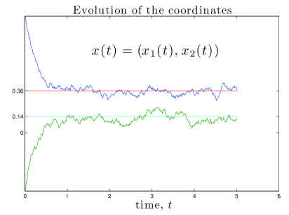
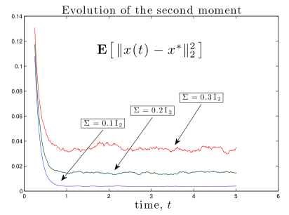
Fig. 1: Evolution of the dynamics (11) with $\mathsf{L}=0$,  $h(x_{1},x_{2})=\log\big{(}e^{(x_{1}-2)}+e^{(x_{2}+1)}\big{)}+0.5(x_{1}+x_{2}-1)^{2}+(x_{1}-x_{2})^{2}$, and initial condition $[x_{1}(0),x_{2}(0)]=(1,-0.5)$. Since $h$ is a sum of convex functions, and the Hessian of the quadratic part of $h$ has eigenvalues $\{2,4\}$, we can take $\gamma$ given by $\gamma(r)=2\,r$, for $r\geq 0$. Plot (a) shows the evolution of the first and second coordinates with $\Sigma=0.1\,\mathrm{I}_{2}$. Plot (b) illustrates the noise-to-state stability property in second moment with respect to $x^{*}=(0.36,0.14)$, where the matrix $\Sigma(t)$ is a constant multiple of the identity. (The expectation is computed averaging over $500$ realizations of the noise.)

Example 11.

(Example 6–revisited: illustration of Corollary 10). Consider again Example 6. Since $\mathrm{V}$ is a $p$th moment NSS-Lyapunov function for (11) with respect to the point $x^{*}$ for $p\in(0,2]$, as shown in Example 9, Corollary 10 implies that

(28) $$\mathbb{E}\big{[}\|x-x^{*}\|_{\text{\scalebox{1.0}{$2$}}}^{p}\big{]} \leq\mu\big{(}\|x_{0}-x^{*}\|_{\text{\scalebox{1.0}{$2$}}},t-t_{0}\big{)}+\theta\Big{(}\max_{t_{0}\leq s\leq t}|\Sigma(s)|_{\text{\scalebox{0.8}{$\mathcal{F}$}}}\Big{)},$$

for all $t\geq t_{0}$, $x_{0}\in{\mathbb{R}}^{n}$, and $p\in(0,2]$, where

$$\mu(r,s)\>=\big{(}2\tilde{\mu}(r^{2},s)\big{)}^{p/2},\quad\theta(r)\>=\big{(}\gamma^{-1}(r^{2})\big{)}^{p/2},$$

and the class $\mathcal{KL}$ function $\tilde{\mu}$ is defined as the solution to the initial value problem (13) with $\eta(r)=\tfrac{1}{2}\gamma^{-1}(r)$. Figure 1 illustrates this noise-to-state stability property. We note that if the function $h$ is strongly convex, i.e., if $\gamma(r)=c_{\gamma}\,r$ for some constant $c_{\gamma}>0$, then $\tilde{\mu}:{\mathbb{R}}_{\geq 0}\times{\mathbb{R}}_{\geq 0}\rightarrow{\mathbb{R}}_{\geq 0}$ becomes $\tilde{\mu}(r,s)=re^{-c_{\gamma}s}$, and $\mu(r,s)=2^{p/2}\,r^{p}e^{-c_{\gamma}p/2\,s}$, so the bound for $\mathbb{E}\big{[}\|x-x^{*}\|_{\text{\scalebox{1.0}{$2$}}}^{p}\big{]}$ in (28) decays exponentially with time to $\theta\big{(}\max_{t_{0}\leq s\leq t}|\Sigma(s)|_{\text{\scalebox{0.8}{$\mathcal{F}$}}}\big{)}$. $\bullet$

4 Refinements of the notion of proper functions

In this section, we analyze in detail the inequalities between functions that appear in the definition of noise-dissipative Lyapunov function, strong NSS-Lyapunov function in probability, and $p$th moment NSS-Lyapunov function. In Section 4.1, we establish that these inequalities can be regarded as equivalence relations. In Section 4.2, we make a complete characterization of the properties of two functions related by these equivalence relations. Finally, in Section 4.3, these results lead us to obtain an alternative formulation of Corollary 10.

4.1 Proper functions and equivalence relations

Here, we provide a refinement of the notion of proper functions with respect to each other. Proper functions play an important role in stability analysis, see e.g., [6, 23].

Definition 12.

(Refinements of the notion of proper functions with respect to each other). Let $\mathcal{D}\subseteq{\mathbb{R}}^{n}$ and the functions $\mathrm{V},\mathrm{W}:\mathcal{D}\rightarrow{\mathbb{R}}_{\geq 0}$ be such that

$$\alpha_{1}(\mathrm{W}(x))\leq\mathrm{V}(x)\leq\alpha_{2}(\mathrm{W}(x)),\quad\forall x\in\mathcal{D},$$

for some functions $\alpha_{1},\,\alpha_{2}:{\mathbb{R}}_{\geq 0}\rightarrow{\mathbb{R}}_{\geq 0}$. Then,

1. if $\alpha_{1},\alpha_{2}\in\mathcal{K}$, we say that $\mathrm{V}$ is $\mathcal{K}$ - dominated by $\mathrm{W}$ in $\mathcal{D}$, and write $\linebreak\mathrm{V}\vartriangleleft^{\text{\scalebox{0.8}{$\mathcal{K}$}}}\mathrm{W}\;\;\text{in}\;\;\mathcal{D}$;

2. if $\alpha_{1},\alpha_{2}\in\mathcal{K}_{\infty}$, we say that $\mathrm{V}$ and $\mathrm{W}$ are $\mathcal{K}_{\infty}$ - proper with respect to each other in $\mathcal{D}$, and write $\mathrm{V}\thicksim^{\text{\scalebox{0.8}{$\mathcal{K}_{\infty}$}}}\mathrm{W}\;\;\text{in}\;\;\mathcal{D}$;

3. if $\alpha_{1},\alpha_{2}\in\mathcal{K}_{\infty}$ are convex and concave, respectively, we say that $\mathrm{V}$ and $\mathrm{W}$ are $\mathcal{K}_{\infty}^{cc}$ - (convex-concave) proper with respect to each other in $\mathcal{D}$, and write $\mathrm{V}\thicksim^{\text{\scalebox{0.8}{$\mathcal{K}_{\infty}^{cc}$}}}\mathrm{W}\;\;\text{in}\;\;\mathcal{D}$;

4. if $\alpha_{1}(r)\triangleq c_{\alpha_{1}}r$ and $\alpha_{2}(r)\triangleq c_{\alpha_{2}}r$, for some constants $c_{\alpha_{1}},c_{\alpha_{2}}>0$, we say that $\mathrm{V}$ and $\mathrm{W}$ are equivalent in $\mathcal{D}$, and write $\mathrm{V}\thicksim\mathrm{W}\;\;\text{in}\;\;\mathcal{D}$.

Note that the relations in Definition 12 are nested, i.e., given $\mathrm{V},\mathrm{W}:\mathcal{D}\rightarrow{\mathbb{R}}_{\geq 0}$, the following chain of implications hold in $\mathcal{D}$ :

(29) $$\mathrm{V}\thicksim\mathrm{W}\,\Rightarrow\,\mathrm{V}\thicksim^{\text{\scalebox{0.8}{$\mathcal{K}_{\infty}^{cc}$}}}\mathrm{W}\,\Rightarrow\,\mathrm{V}\thicksim^{\text{\scalebox{0.8}{$\mathcal{K}_{\infty}$}}}\mathrm{W}\,\Rightarrow\,\mathrm{V}\vartriangleleft^{\text{\scalebox{0.8}{$\mathcal{K}$}}}\mathrm{W}.$$

Also, note that if $\mathrm{W}(x)=\|x\|_{\text{\scalebox{1.0}{$2$}}}$, $\mathcal{D}$ is a neighborhood of $0$, and $\alpha_{1},\alpha_{2}$ are class $\mathcal{K}$, then we recover the notion of $\mathrm{V}$ being a proper function [6]. If $\mathcal{D}={\mathbb{R}}^{n}$, and $\mathrm{V}$ and $\mathrm{W}$ are seminorms, then the relation $\thicksim$ corresponds to the concept of equivalent seminorms.

The relation $\thicksim^{\text{\scalebox{0.8}{$\mathcal{K}_{\infty}$}}}$ is relevant for ISS and NSS in probability, whereas the relation $\thicksim^{\text{\scalebox{0.8}{$\mathcal{K}_{\infty}^{cc}$}}}$ is important for $p$th moment NSS. The latter is because the inequalities in $\thicksim^{\text{\scalebox{0.8}{$\mathcal{K}_{\infty}^{cc}$}}}$ are still valid, thanks to Jensen inequality, if we substitute $\mathrm{V}$ and $\mathrm{W}$ by their expectations along a stochastic process. Another fact about the relation $\thicksim^{\text{\scalebox{0.8}{$\mathcal{K}_{\infty}^{cc}$}}}$ is that $\alpha_{1},\alpha_{2}\in\mathcal{K}_{\infty}$, convex and concave, respectively, must be asymptotically linear if $\mathrm{V}(\mathcal{D})\supseteq[s_{0},\infty)$, for some $s_{0}\geq 0$, so that $\alpha_{1}(s)\leq\alpha_{2}(s)$ for all $s\geq s_{0}$. This follows from Lemma A.1.

Remark 13.

(Quadratic forms in a constrained domain). It is sometimes convenient to view the functions $\mathrm{V},\mathrm{W}:\mathcal{D}\rightarrow{\mathbb{R}}_{\geq 0}$ as defined in a domain where their functional expression becomes simpler. To make this idea precise, assume there exist $i:\mathcal{D}\subset{\mathbb{R}}^{n}\rightarrow{\mathbb{R}}^{m}$, with $m\geq n$, and $\hat{\mathrm{V}},\hat{\mathrm{W}}:\hat{\mathcal{D}}\rightarrow{\mathbb{R}}_{\geq 0}$, where $\hat{\mathcal{D}}=i(\mathcal{D})$, such that $\mathrm{V}=\hat{\mathrm{V}}\circ i$ and $\mathrm{W}=\hat{\mathrm{W}}\circ i$. If this is the case, then the existence of $\alpha_{1},\,\alpha_{2}:{\mathbb{R}}_{\geq 0}\to{\mathbb{R}}_{\geq 0}$ such that $\alpha_{1}\big{(}\hat{\mathrm{W}}(\hat{x})\big{)}\leq\hat{\mathrm{V}}(\hat{x})\leq\alpha_{2}\big{(}\hat{\mathrm{W}}(\hat{x})\big{)}$, for all $\hat{x}\in\hat{\mathcal{D}}$, implies that $\alpha_{1}\big{(}\mathrm{W}({x})\big{)}\leq\mathrm{V}({x})\leq\alpha_{2}\big{(}\mathrm{W}({x})\big{)}$, for all $x\in\mathcal{D}$. The reason is that for any $x\in\mathcal{D}$ there exists $\hat{x}\in\hat{\mathcal{D}}$, given by $\hat{x}=i(x)$, such that $\mathrm{V}(x)=\hat{\mathrm{V}}(\hat{x})$ and $\mathrm{W}(x)=\hat{\mathrm{W}}(\hat{x})$, so

$$\alpha_{1}\big{(}\mathrm{W}(x)\big{)}=\alpha_{1}\big{(}\hat{\mathrm{W}}(\hat{x})\big{)}\leq\mathrm{V}(x)=\hat{\mathrm{V}}(\hat{x})\leq\alpha_{2}\big{(}\hat{\mathrm{W}}(\hat{x})\big{)}=\alpha_{2}\big{(}\mathrm{W}(x)\big{)}.$$

Consequently, if any of the relations given in Definition 12 is satisfied by $\hat{\mathrm{V}}$, $\hat{\mathrm{W}}$ in $\hat{\mathcal{D}}$, then the corresponding relation is satisfied by $\mathrm{V}$, $\mathrm{W}$ in $\mathcal{D}$. For instance, in some scenarios this procedure can allow us to rewrite the original functions $\mathrm{V}$, $\mathrm{W}$ as quadratic forms $\hat{\mathrm{V}}$, $\hat{\mathrm{W}}$ in a constrained set of an extended Euclidean space, where it is easier to establish the appropriate relation between the functions. We make use of this observation in Section 4.3 below. $\bullet$

Lemma 14.

(Powers of seminorms with the same nullspace). Let $A$ and $B$ in $\mathbb{R}^{m\times n}$ be nonzero matrices with the same nullspace, $\operatorname{\mathcal{N}}(A)=\operatorname{\mathcal{N}}(B)$. Then, for any $p,q>0$, the inequalities $\alpha_{1}\big{(}\|x\|_{\text{\scalebox{1.0}{$A$}}}^{p}\big{)}\leq\|x\|_{\text{\scalebox{1.0}{$B$}}}^{q}\leq\alpha_{2}\big{(}\|x\|_{\text{\scalebox{1.0}{$A$}}}^{p}\big{)}$ are verified with

$$\alpha_{1}(r)\triangleq\Big{(}\frac{\lambda_{n-k}(B^{\text{\scalebox{0.8}{$T$}}}B)}{\operatorname{\lambda_{\text{max}}}(A^{\text{\scalebox{0.8}{$T$}}}A)}\Big{)}^{\frac{q}{2}}\,r^{q/p};\quad\alpha_{2}(r)\triangleq\Big{(}\frac{\operatorname{\lambda_{\text{max}}}(B^{\text{\scalebox{0.8}{$T$}}}B)}{\lambda_{n-k}(A^{\text{\scalebox{0.8}{$T$}}}A)}\Big{)}^{\frac{q}{2}}\,r^{q/p},$$

where $k\triangleq\dim(\operatorname{\mathcal{N}}(A))$. In particular, $\|.\|_{\text{\scalebox{1.0}{$A$}}}^{p}\thicksim\|.\|_{\text{\scalebox{1.0}{$B$}}}^{p}$  and  $\|.\|_{\text{\scalebox{1.0}{$A$}}}^{p}\thicksim^{\text{\scalebox{0.8}{$\mathcal{K}_{\infty}$}}}\|.\|_{\text{\scalebox{1.0}{$B$}}}^{q}$  in  ${\mathbb{R}}^{n}$ for any real numbers $p,q>0$.

Proof.

For $\mathcal{U}\triangleq\operatorname{\mathcal{N}}(A)$, write any $x\in{\mathbb{R}}^{n}$ as $x=x_{\text{\scalebox{0.8}{$\mathcal{U}$}}}+x_{\text{\scalebox{0.8}{$\mathcal{U}^{\bot}$}}}$, where $x_{\text{\scalebox{0.8}{$\mathcal{U}$}}}\in\mathcal{U}$ and $x_{\text{\scalebox{0.8}{$\mathcal{U}^{\bot}$}}}\in\{x\in{\mathbb{R}}^{n}\,:\,x^{\text{\scalebox{0.8}{$T$}}}u=0\;,\forall u\in\mathcal{U}\}$, so that $Ax=A(x_{\text{\scalebox{0.8}{$\mathcal{U}$}}}+x_{\text{\scalebox{0.8}{$\mathcal{U}^{\bot}$}}})=Ax_{\text{\scalebox{0.8}{$\mathcal{U}^{\bot}$}}}$ and $Bx=Bx_{\text{\scalebox{0.8}{$\mathcal{U}^{\bot}$}}}$ because $\operatorname{\mathcal{N}}(A)=\operatorname{\mathcal{N}}(B)=\mathcal{U}$. Using the formulas for the eigenvalues in [5, p. 178], we see that the next chain of inequalities hold:

$$\alpha_{1}\big{(}\|x\|_{\text{\scalebox{1.0}{$A$}}}^{p}\big{)}=\alpha_{1}\Big{(}\big{(}x_{\text{\scalebox{0.8}{$\mathcal{U}^{\bot}$}}}^{\text{\scalebox{0.8}{$T$}}}A^{\text{\scalebox{0.8}{$T$}}}Ax_{\text{\scalebox{0.8}{$\mathcal{U}^{\bot}$}}}\big{)}^{\frac{p}{2}}\Big{)}\leq\alpha_{1}\Big{(}\big{(}\operatorname{\lambda_{\text{max}}}(A^{\text{\scalebox{0.8}{$T$}}}A)x_{\text{\scalebox{0.8}{$\mathcal{U}^{\bot}$}}}^{\text{\scalebox{0.8}{$T$}}}x_{\text{\scalebox{0.8}{$\mathcal{U}^{\bot}$}}}\big{)}^{\frac{p}{2}}\Big{)}$$

$$\leq\big{(}\lambda_{n-k}(B^{\text{\scalebox{0.8}{$T$}}}B)x_{\text{\scalebox{0.8}{$\mathcal{U}^{\bot}$}}}^{\text{\scalebox{0.8}{$T$}}}x_{\text{\scalebox{0.8}{$\mathcal{U}^{\bot}$}}}\big{)}^{\frac{q}{2}}\leq\big{(}x_{\text{\scalebox{0.8}{$\mathcal{U}^{\bot}$}}}^{\text{\scalebox{0.8}{$T$}}}B^{\text{\scalebox{0.8}{$T$}}}Bx_{\text{\scalebox{0.8}{$\mathcal{U}^{\bot}$}}}\big{)}^{\frac{q}{2}}\leq\big{(}\operatorname{\lambda_{\text{max}}}(B^{\text{\scalebox{0.8}{$T$}}}B)x_{\text{\scalebox{0.8}{$\mathcal{U}^{\bot}$}}}^{\text{\scalebox{0.8}{$T$}}}x_{\text{\scalebox{0.8}{$\mathcal{U}^{\bot}$}}}\big{)}^{\frac{q}{2}}$$

$$\leq\alpha_{2}\Big{(}\big{(}\lambda_{n-k}(A^{\text{\scalebox{0.8}{$T$}}}A)x_{\text{\scalebox{0.8}{$\mathcal{U}^{\bot}$}}}^{\text{\scalebox{0.8}{$T$}}}x_{\text{\scalebox{0.8}{$\mathcal{U}^{\bot}$}}}\big{)}^{\frac{p}{2}}\Big{)}\leq\alpha_{2}\Big{(}\big{(}x_{\text{\scalebox{0.8}{$\mathcal{U}^{\bot}$}}}^{\text{\scalebox{0.8}{$T$}}}A^{\text{\scalebox{0.8}{$T$}}}Ax_{\text{\scalebox{0.8}{$\mathcal{U}^{\bot}$}}}\big{)}^{\frac{p}{2}}\Big{)}=\alpha_{2}\big{(}\|x\|_{\text{\scalebox{1.0}{$A$}}}^{p}\big{)},$$

where $\|x\|_{\text{\scalebox{1.0}{$B$}}}^{q}=\big{(}x_{\text{\scalebox{0.8}{$\mathcal{U}^{\bot}$}}}^{\text{\scalebox{0.8}{$T$}}}B^{\text{\scalebox{0.8}{$T$}}}Bx_{\text{\scalebox{0.8}{$\mathcal{U}^{\bot}$}}}\big{)}^{\frac{q}{2}}$. From this we conclude that $\|.\|_{\text{\scalebox{1.0}{$A$}}}^{p}\thicksim^{\text{\scalebox{0.8}{$\mathcal{K}_{\infty}$}}}\|.\|_{\text{\scalebox{1.0}{$B$}}}^{q}$ in ${\mathbb{R}}^{n}$. Finally, when $p=q$, the class $\mathcal{K}_{\infty}$ functions $\alpha_{1}$, $\alpha_{2}$ in the statement are linear, so we obtain that $\|.\|_{\text{\scalebox{1.0}{$A$}}}^{p}\thicksim\|.\|_{\text{\scalebox{1.0}{$B$}}}^{p}$ in ${\mathbb{R}}^{n}$. ∎

Next we show that $\thicksim^{\text{\scalebox{0.8}{$\mathcal{K}_{\infty}$}}}$ and $\thicksim^{\text{\scalebox{0.8}{$\mathcal{K}_{\infty}^{cc}$}}}$ are reflexive, symmetric, and transitive, and hence define equivalence relations.

Lemma 15.

(The $\mathcal{K}_{\infty}$- and $\mathcal{K}_{\infty}^{cc}$-proper relations are equivalence relations). The relations $\thicksim^{\text{\scalebox{0.8}{$\mathcal{K}_{\infty}$}}}$ and $\thicksim^{\text{\scalebox{0.8}{$\mathcal{K}_{\infty}^{cc}$}}}$ in any set $\mathcal{D}\subseteq{\mathbb{R}}^{n}$ are both equivalence relations.

Proof.

For convenience, we represent both relations by $\thicksim^{*}$. Both are reflexive, i.e., $\mathrm{V}\thicksim^{*}\mathrm{V}$, because one can take $\alpha_{1}(r)=\alpha_{2}(r)=r$ noting that a linear function is both convex and concave. Both are symmetric, i.e., $\mathrm{V}\thicksim^{*}\mathrm{W}$ if and only if $\mathrm{W}\thicksim^{*}\mathrm{V}$, because if $\alpha_{1}\circ\mathrm{W}\leq\mathrm{V}\leq\alpha_{2}\circ\mathrm{W}$ in $\mathcal{D}$, then $\alpha_{2}^{-1}\circ\mathrm{V}\leq\mathrm{W}\leq\alpha_{1}^{-1}\circ\mathrm{V}$ in $\mathcal{D}$. In the case of $\thicksim^{\text{\scalebox{0.8}{$\mathcal{K}_{\infty}$}}}$, the inverse of a class $\mathcal{K}_{\infty}$ function is class $\mathcal{K}_{\infty}$. Additionally, in the case of $\thicksim^{\text{\scalebox{0.8}{$\mathcal{K}_{\infty}^{cc}$}}}$, if $\alpha\in\mathcal{K}_{\infty}$ is convex (respectively, concave), then $\alpha^{-1}\in\mathcal{K}_{\infty}$ is concave (respectively, convex). Finally, both are transitive, i.e., $\mathrm{U}\thicksim^{*}\mathrm{V}$ and $\mathrm{V}\thicksim^{*}\mathrm{W}$ imply $\mathrm{U}\thicksim^{*}\mathrm{W}$, because if $\alpha_{1}\circ\mathrm{V}\leq\mathrm{U}\leq\alpha_{2}\circ\mathrm{V}$ and $\tilde{\alpha}_{1}\circ\mathrm{W}\leq\mathrm{V}\leq\tilde{\alpha}_{2}\circ\mathrm{W}$ in $\mathcal{D}$, then $\alpha_{1}\circ\tilde{\alpha}_{1}\circ\mathrm{W}\leq\mathrm{U}\leq\alpha_{2}\circ\tilde{\alpha}_{2}\circ\mathrm{W}$ in $\mathcal{D}$. In the case of $\thicksim^{\text{\scalebox{0.8}{$\mathcal{K}_{\infty}$}}}$, the composition of two class $\mathcal{K}_{\infty}$ functions is class $\mathcal{K}_{\infty}$. Additionally, in the case of $\thicksim^{\text{\scalebox{0.8}{$\mathcal{K}_{\infty}^{cc}$}}}$, if $\alpha_{1},\alpha_{2}\in\mathcal{K}_{\infty}$ are both convex (respectively, concave), then the compositions $\alpha_{1}\circ\alpha_{2}$ and $\alpha_{2}\circ\alpha_{1}$ belong to $\mathcal{K}_{\infty}$ and are convex (respectively, concave), as explained in Section 2.2. ∎

Remark 16.

(The relation $\vartriangleleft^{\text{\scalebox{0.8}{$\mathcal{K}$}}}$ is not an equivalence relation). The proof above also shows that the relation $\vartriangleleft^{\text{\scalebox{0.8}{$\mathcal{K}$}}}$ is reflexive and transitive. However, it is not symmetric: consider $\mathrm{V},\mathrm{W}\in\mathcal{C}({\mathbb{R}}^{n};{\mathbb{R}}_{{\text{\scalebox{0.7}{$\geq 0$}}}})$ given by $\mathrm{V}(x)=1-e^{-\|x\|_{\text{\scalebox{1.0}{$2$}}}}$ and $\mathrm{W}(x)=\|x\|_{\text{\scalebox{1.0}{$2$}}}$. Clearly, $\mathrm{V}\vartriangleleft^{\text{\scalebox{0.8}{$\mathcal{K}$}}}\mathrm{W}$ in ${\mathbb{R}}^{n}$ by taking $\alpha_{1}=\alpha_{2}=\alpha\in\mathcal{K}$, with $\alpha(s)=1-e^{-s}$. On the other hand, if there exist $\tilde{\alpha}_{1},\tilde{\alpha}_{2}\in\mathcal{K}$ such that $\tilde{\alpha}_{1}(\mathrm{V}(x))\leq\mathrm{W}(x)\leq\tilde{\alpha}_{2}(\mathrm{V}(x))$ for all $x\in{\mathbb{R}}^{n}$, then we reach the contradiction, by continuity of $\tilde{\alpha}_{2}$, that $\lim_{\|x\|_{\text{\scalebox{1.0}{$2$}}}\to\infty}\|x\|_{\text{\scalebox{1.0}{$2$}}}\leq\tilde{\alpha}_{2}\big{(}\lim_{\|x\|_{\text{\scalebox{1.0}{$2$}}}\to\infty}\big{(}1-e^{-\|x\|_{\text{\scalebox{1.0}{$2$}}}}\big{)}\big{)}=\tilde{\alpha}_{2}(1)<\infty$. $\bullet$

4.2 Characterization of proper functions with respect to each other

In this section, we provide a complete characterization of the properties that two functions must satisfy to be related by the equivalence relations defined in Section 4.1. For $\mathcal{D}\subseteq{\mathbb{R}}^{n}$, consider $\mathrm{V}_{1},\mathrm{V}_{2}:\mathcal{D}\rightarrow{\mathbb{R}}_{\geq 0}$. Given a real number $p>0$, define

$$\phi_{\text{\scalebox{0.8}{$p$}}}(s) \triangleq\sup_{\{y\in\mathcal{D}\,:\,\mathrm{V}_{2}(y)\,\leq\sqrt[p]{s}\}}\mathrm{V}_{1}(y),$$

$$\psi_{\text{\scalebox{0.8}{$p$}}}(s) \triangleq\inf_{\{y\in\mathcal{D}\,:\,\mathrm{V}_{2}(y)\,\geq\sqrt[p]{s}\}}\mathrm{V}_{1}(y),$$

for $s\geq 0$. The value $\phi_{\text{\scalebox{0.8}{$p$}}}(s)$ gives the supremum of the function $\mathrm{V}_{1}$ in the $\sqrt[p]{s}$ - sublevel set of $\mathrm{V}_{2}$, and $\psi_{\text{\scalebox{0.8}{$p$}}}(s)$ is the infimum of $\mathrm{V}_{1}$ in the $\sqrt[p]{s}$ - superlevel set of $\mathrm{V}_{2}$. Thus, the functions $\phi_{\text{\scalebox{0.8}{$p$}}}$ and $\psi_{\text{\scalebox{0.8}{$p$}}}$ satisfy

(30) $$\psi_{\text{\scalebox{0.8}{$p$}}}\big{(}\mathrm{V}_{2}(x)^{p}\big{)}\,=\,\!\!\!\inf_{\begin{subarray}{c}\{y\in\mathcal{D}\,:\\ \mathrm{V}_{2}(y)\,\geq\,\mathrm{V}_{2}(x)\}\end{subarray}}\!\!\!\mathrm{V}_{1}(y)\,\leq\,\mathrm{V}_{1}(x)\,\leq\,\!\!\!\sup_{\begin{subarray}{c}\{y\in\mathcal{D}\,:\\ \mathrm{V}_{2}(y)\,\leq\,\mathrm{V}_{2}(x)\}\end{subarray}}\!\!\!\mathrm{V}_{1}(y)\,=\,\phi_{\text{\scalebox{0.8}{$p$}}}\big{(}\mathrm{V}_{2}(x)^{p}\big{)},$$

for all $x\in\mathcal{D}$, which suggests $\phi_{\text{\scalebox{0.8}{$p$}}}$ and $\psi_{\text{\scalebox{0.8}{$p$}}}$ as pre-comparison functions to construct $\alpha_{1}$ and $\alpha_{2}$ in Definition 12. To this end, we find it useful to formulate the following properties of the function $\mathrm{V}_{1}$ with respect to $\mathrm{V}_{2}$:

$\operatorname{P0}$: The set $\{x\in\mathcal{D}:\mathrm{V}_{2}(x)=s\}$ is nonempty for all $s\geq 0$.

$\operatorname{P1}$: The nullsets of $\mathrm{V}_{1}$ and $\mathrm{V}_{2}$ are the same, i.e., $\{x\in\mathcal{D}\,:\,\mathrm{V}_{1}(x)=0\}=\{x\in\mathcal{D}\,:\,\mathrm{V}_{2}(x)=0\}$.

$\operatorname{P2}$: The function $\phi_{\text{\scalebox{0.8}{$1$}}}$ is locally bounded in ${\mathbb{R}}_{\geq 0}$ and right continuous at $0$, and $\psi_{\text{\scalebox{0.8}{$1$}}}$ is positive definite.

$\operatorname{P3}$: The next limit holds: $\lim_{s\to\infty}\psi_{\text{\scalebox{0.8}{$1$}}}(s)=\infty$.

$\operatorname{P4}$ (as a function of $p>0$): The asymptotic behavior of $\phi_{\text{\scalebox{0.8}{$p$}}}$ and $\psi_{\text{\scalebox{0.8}{$p$}}}$ is such that $\phi_{\text{\scalebox{0.8}{$p$}}}(s)$ and $s^{2}/\psi_{\text{\scalebox{0.8}{$p$}}}(s)$ are both in $\mathcal{O}(s)$ as $s\to\infty$.

The next result shows that these properties completely characterize whether the functions $\mathrm{V}_{1}$ and $\mathrm{V}_{2}$ are related through the equivalence relations defined in Section 4.1. This result generalizes [6, Lemma 4.3] in several ways: the notions of proper functions considered here are more general and are not necessarily restricted to a relationship between an arbitrary function and the distance to a compact set.

Theorem 17.

(Characterizations of proper functions with respect to each other). Let $\mathrm{V}_{1},\mathrm{V}_{2}:\mathcal{D}\rightarrow{\mathbb{R}}_{\geq 0}$, and assume $\mathrm{V}_{2}$ satisfies $\operatorname{P0}$. Then

1. $\mathrm{V}_{1}$ satisfies $\{\operatorname{P}$i$\}_{i=1}^{2}$ with respect to $\mathrm{V}_{2}$  $\Leftrightarrow$  $\mathrm{V}_{1}\,\vartriangleleft^{\text{\scalebox{0.8}{$\mathcal{K}$}}}\,\mathrm{V}_{2}$ in $\mathcal{D}$ ;

2. $\mathrm{V}_{1}$ satisfies $\{\operatorname{P}$i$\}_{i=1}^{3}$ with respect to $\mathrm{V}_{2}$  $\Leftrightarrow$  $\mathrm{V}_{1}\thicksim^{\text{\scalebox{0.8}{$\mathcal{K}_{\infty}$}}}\mathrm{V}_{2}$ in $\mathcal{D}$ ;

3. $\mathrm{V}_{1}$ satisfies $\{\operatorname{P}$i$\}_{i=1}^{4}$ with respect to $\mathrm{V}_{2}$ for $p>0$  $\Leftrightarrow$  $\mathrm{V}_{1}\thicksim^{\text{\scalebox{0.8}{$\mathcal{K}_{\infty}^{cc}$}}}\mathrm{V}_{2}^{p}$ in $\mathcal{D}$.

Proof.

We begin by establishing a few basic facts about the pre-comparison functions $\psi_{\text{\scalebox{0.8}{$p$}}}$ and $\phi_{\text{\scalebox{0.8}{$p$}}}$. By definition and by $\operatorname{P0}$, it follows that $0\leq\psi_{\text{\scalebox{0.8}{$1$}}}(s)\leq\phi_{\text{\scalebox{0.8}{$1$}}}(s)$ for all $s\geq 0$. Since $\phi_{\text{\scalebox{0.8}{$1$}}}$ is locally bounded by $\operatorname{P2}$, then so is $\psi_{\text{\scalebox{0.8}{$1$}}}$. In particular, $\phi_{\text{\scalebox{0.8}{$1$}}}$ and $\psi_{\text{\scalebox{0.8}{$1$}}}$ are well defined in ${\mathbb{R}}_{\geq 0}$. Moreover, both $\phi_{\text{\scalebox{0.8}{$1$}}}$ and $\psi_{\text{\scalebox{0.8}{$1$}}}$ are nondecreasing because if $s_{2}\geq s_{1}$, then the supremum is taken in a larger set, $\{x\in\mathcal{D}:\mathrm{V}_{2}(x)\leq s_{2}\}\supseteq\{x\in\mathcal{D}:\mathrm{V}_{2}(x)\leq s_{1}\}$, and the infimum is taken in a smaller set, $\{x\in\mathcal{D}:\mathrm{V}_{2}(x)\geq s_{2}\}\subseteq\{x\in\mathcal{D}:\mathrm{V}_{2}(x)\geq s_{1}\}$. Furthermore, for any $q>0$, the functions $\phi_{\text{\scalebox{0.8}{$q$}}}$ and $\psi_{\text{\scalebox{0.8}{$q$}}}$ are also monotonic and positive definite because $\phi_{\text{\scalebox{0.8}{$q$}}}(s)=\phi_{\text{\scalebox{0.8}{$1$}}}(\sqrt[q]{s})$ and $\psi_{\text{\scalebox{0.8}{$q$}}}(s)=\psi_{\text{\scalebox{0.8}{$1$}}}(\sqrt[q]{s})$ for all $s\geq 0$. We now use these properties of the pre-comparison functions to construct $\alpha_{1}$, $\alpha_{2}$ in Definition 12 required by the implications from left to right in each statement.

Proof of (i) ($\Rightarrow$). To show the existence of $\alpha_{2}\in\mathcal{K}$ such that $\alpha_{2}(s)\geq\phi_{\text{\scalebox{0.8}{$1$}}}(s)$ for all $s\in{\mathbb{R}}_{\geq 0}$, we proceed as follows. Since $\phi_{\text{\scalebox{0.8}{$1$}}}$ is locally bounded and nondecreasing, given a strictly increasing sequence $\{b_{k}\}_{k\geq 1}\subseteq{\mathbb{R}}_{\geq 0}$ with $\lim_{k\to\infty}b_{k}=\infty$, we choose the sequence $\{M_{k}\}_{k\geq 1}\subseteq{\mathbb{R}}_{\geq 0}$, setting $M_{0}=0$, in the following way:

(31) $$M_{k}\triangleq\max\Big{\{}\sup_{s\in[0,b_{k}]}\phi_{\text{\scalebox{0.8}{$1$}}}(s)\,,\>M_{k-1}+1/k^{2}\Big{\}}=\max\big{\{}\phi_{\text{\scalebox{0.8}{$1$}}}(b_{k})\,,\>M_{k-1}+1/k^{2}\big{\}}.$$

This choice guarantees that $\{M_{k}\}_{k\geq 1}$ is strictly increasing and, for each $k\geq 1$,

(32) $$0\leq M_{k}-\phi_{\text{\scalebox{0.8}{$1$}}}(b_{k})\leq\sum_{i=1}^{k}\frac{1}{i^{2}}\leq\pi^{2}/6.$$

Also, since $\phi_{\text{\scalebox{0.8}{$1$}}}$ is right continuous at $0$, we can choose $b_{1}>0$ such that there exists $\alpha_{2}:[0,b_{1}]\rightarrow{\mathbb{R}}_{\geq 0}$ continuous, positive definite and strictly increasing, satisfying that $\alpha_{2}(s)\geq\phi_{\text{\scalebox{0.8}{$1$}}}(s)$ for all $s\in[0,b_{1}]$ and with $\alpha_{2}(b_{1})=M_{2}$. (This is possible because the only function that cannot be upper bounded by an arbitrary continuous function in some arbitrarily small interval $[0,b_{1}]$ is the function that has a jump at $0$.) The rest of the construction is explicit. We define $\alpha_{2}$ as a piecewise linear function in $(b_{1},\infty)$ in the following way: for each $k\geq 2$, we define

$$\alpha_{2}(s)\triangleq\alpha_{2}(b_{k-1})+\frac{M_{k+1}-\alpha_{2}(b_{k-1})}{b_{k}-b_{k-1}}\,(s-b_{k-1}),\qquad\forall s\in(b_{k-1},b_{k}].$$

The resulting $\alpha_{2}$ is continuous by construction. Also, $\alpha_{2}(b_{1})=M_{2}$, so that, inductively, $\alpha_{2}(b_{k-1})=M_{k}$ for $k\geq 2$. Two facts now follow: first, $M_{k+1}-\alpha_{2}(b_{k-1})=M_{k+1}-M_{k}\geq 1/(k+1)^{2}$ for $k\geq 2$, so $\alpha_{2}$ has positive slope in each interval $(b_{k-1},b_{k}]$ and thus is strictly increasing in $(b_{1},\infty)$; second, $\alpha_{2}(s)>\alpha_{2}(b_{k-1})=M_{k}\geq\phi_{\text{\scalebox{0.8}{$1$}}}(b_{k})\geq\phi_{\text{\scalebox{0.8}{$1$}}}(s)$ for all $s\in(b_{k-1},b_{k}]$, for each $k\geq 2$, so $\alpha_{2}(s)\geq\phi_{\text{\scalebox{0.8}{$1$}}}(s)$ for all $s\in(b_{1},\infty)$.

We have left to show the existence of $\alpha_{1}\in\mathcal{K}$ such that $\alpha_{1}(s)\leq\psi_{\text{\scalebox{0.8}{$1$}}}(s)$ for all $s\in{\mathbb{R}}_{\geq 0}$. First, since $0\leq\psi_{\text{\scalebox{0.8}{$1$}}}(s)\leq\phi_{\text{\scalebox{0.8}{$1$}}}(s)$ for all $s\geq 0$ by definition and by $\operatorname{P0}$, using the sandwich theorem [11, p. 107], we derive that $\psi_{\text{\scalebox{0.8}{$1$}}}$ is right continuous at $0$ the same as $\phi_{\text{\scalebox{0.8}{$1$}}}$. In addition, since $\psi_{\text{\scalebox{0.8}{$1$}}}$ is nondecreasing, it can only have a countable number of jump discontinuities (none of them at $0$). Therefore, we can pick $c_{1}>0$ such that a continuous and nondecreasing function $\hat{\psi}_{\text{\scalebox{0.8}{$1$}}}$ can be constructed in $[0,c_{1})$ by removing the jumps of $\psi_{\text{\scalebox{0.8}{$1$}}}$, so that $\hat{\psi}_{\text{\scalebox{0.8}{$1$}}}(s)\leq\psi_{\text{\scalebox{0.8}{$1$}}}(s)$. Moreover, since $\psi_{\text{\scalebox{0.8}{$1$}}}$ is positive definite and right continuous at $0$, then $\hat{\psi}_{\text{\scalebox{0.8}{$1$}}}$ is also positive definite. Thus, there exists $\alpha_{1}$ in $[0,c_{1})$ continuous, positive definite, and strictly increasing, such that, for some $r<1$,

(33) $$\alpha_{1}(s)\leq r\hat{\psi}_{\text{\scalebox{0.8}{$1$}}}(s)\leq r\psi_{\text{\scalebox{0.8}{$1$}}}(s)$$

for all $s\in[0,c_{1})$. To extend $\alpha_{1}$ to a function in class $\mathcal{K}$ in ${\mathbb{R}}_{\geq 0}$, we follow a similar strategy as for $\alpha_{2}$. Given a strictly increasing sequence $\{c_{k}\}_{k\geq 2}\subseteq{\mathbb{R}}_{\geq 0}$ with $\lim_{k\to\infty}c_{k}=\infty$, we define a sequence $\{m_{k}\}_{k\geq 1}\subseteq{\mathbb{R}}_{\geq 0}$ in the following way:

(34) $$m_{k}\triangleq\inf_{s\in[c_{k},c_{k+1})}\psi_{\text{\scalebox{0.8}{$1$}}}(s)-\tfrac{\psi_{\text{\scalebox{0.8}{$1$}}}(c_{1})-\alpha_{1}(c_{1})}{1+k^{2}}=\psi_{\text{\scalebox{0.8}{$1$}}}(c_{k})-\tfrac{\psi_{\text{\scalebox{0.8}{$1$}}}(c_{1})-\alpha_{1}(c_{1})}{1+k^{2}}.$$

Next we define $\alpha_{1}$ in $[c_{1},\infty)$ as the piecewise linear function

$$\alpha_{1}(s)\triangleq\alpha_{1}(c_{k})+\frac{m_{k}-\alpha_{1}(c_{k})}{c_{k+1}-c_{k}}\,(s-c_{k}),\qquad\forall s\in[c_{k},c_{k+1}),$$

for all $k\geq 1$, so $\alpha_{1}$ is continuous by construction. It is also strictly increasing because $\alpha_{1}(c_{2})=m_{1}=(\psi_{\text{\scalebox{0.8}{$1$}}}(c_{1})+\alpha_{1}(c_{1}))/2>\alpha_{1}(c_{1})$ by (33), and also, for each $k\geq 2$, the slopes are positive because $m_{k}-\alpha_{1}(c_{k})=m_{k}-m_{k-1}>0$ (due to the fact that $\{m_{k}\}_{k\geq 1}$ in (34) is strictly increasing because $\psi_{\text{\scalebox{0.8}{$1$}}}$ is nondecreasing). Finally, $\alpha_{1}(s)<\alpha_{1}(c_{k+1})=m_{k}<\psi_{\text{\scalebox{0.8}{$1$}}}(c_{k})\leq\psi_{\text{\scalebox{0.8}{$1$}}}(s)$ for all $s\in[c_{k},c_{k+1})$, for all $k\geq 1$ by (34).

Equipped with $\alpha_{1}$, $\alpha_{2}$ as defined above, and as a consequence of (30), we have that

(35) $$\alpha_{1}(\mathrm{V}_{2}(x)) \,\leq\psi_{\text{\scalebox{0.8}{$1$}}}(\mathrm{V}_{2}(x))\leq\mathrm{V}_{1}(x)\leq\phi_{\text{\scalebox{0.8}{$1$}}}(\mathrm{V}_{2}(x))\leq\alpha_{2}(\mathrm{V}_{2}(x)),\quad\forall x\in\mathcal{D}.$$

This concludes the proof of (i) ($\Rightarrow$).

As a preparation for (ii)-(iii) ($\Rightarrow$), and assuming $\operatorname{P3}$, we derive two facts regarding the functions $\alpha_{1}$ and $\alpha_{2}$ constructed above. First, we establish that

(36) $$\alpha_{2}(s)\in\mathcal{O}(\phi_{\text{\scalebox{0.8}{$1$}}}(s))\;\,\text{as}\;\,s\to\infty.$$

To show this, we argue that

(37) $$\lim_{k\to\infty}\,\sup_{s\in(b_{k-1},b_{k}]}\big{(}\alpha_{2}(s)-\phi_{\text{\scalebox{0.8}{$1$}}}(s)\big{)}\leq\lim_{k\to\infty}\big{(}\phi_{\text{\scalebox{0.8}{$1$}}}(b_{k+1})-\phi_{\text{\scalebox{0.8}{$1$}}}(b_{k-1})\big{)}+\pi^{2}/6,$$

so that there exist $C,s_{1}>0$ such that $\alpha_{2}(s)\leq 3\phi_{\text{\scalebox{0.8}{$1$}}}(s)+C$, for all $s\geq s_{1}$. Thus, noting that $\lim_{s\to\infty}\phi_{\text{\scalebox{0.8}{$1$}}}(s)=\infty$ as a consequence of $\operatorname{P3}$, the expression (36) follows. To establish (37), we use the monotonicity of $\alpha_{2}$ and $\phi_{\text{\scalebox{0.8}{$1$}}}$, (31) and (32). For $k\geq 2$,

$$\sup_{s\in(b_{k-1},b_{k}]}\big{(}\alpha_{2}(s)-\phi_{\text{\scalebox{0.8}{$1$}}}(s)\big{)}\leq\alpha_{2}(b_{k})-\phi_{\text{\scalebox{0.8}{$1$}}}(b_{k-1})=M_{k+1}-\phi_{\text{\scalebox{0.8}{$1$}}}(b_{k-1})$$

$$=\, \max\big{\{}\phi_{\text{\scalebox{0.8}{$1$}}}(b_{k+1})-\phi_{\text{\scalebox{0.8}{$1$}}}(b_{k-1})\,,\>M_{k}+1/(k+1)^{2}-\phi_{\text{\scalebox{0.8}{$1$}}}(b_{k-1})\big{\}}$$

$$\leq\, \max\big{\{}\phi_{\text{\scalebox{0.8}{$1$}}}(b_{k+1})-\phi_{\text{\scalebox{0.8}{$1$}}}(b_{k-1})\,,\>\phi_{\text{\scalebox{0.8}{$1$}}}(b_{k})+\pi^{2}/6+1/(k+1)^{2}-\phi_{\text{\scalebox{0.8}{$1$}}}(b_{k-1})\big{\}}.$$

Second, the construction of $\alpha_{1}$ guarantees that

(38) $$\psi_{\text{\scalebox{0.8}{$1$}}}(s)\in\mathcal{O}(\alpha_{1}(s))\;\,\text{as}\;\,s\to\infty,$$

because, as we show next,

(39) $$\lim_{k\to\infty}\,\sup_{s\in[c_{k},c_{k+1})}\big{(}\psi_{\text{\scalebox{0.8}{$1$}}}(s)-\alpha_{1}(s)\big{)}\leq\lim_{k\to\infty}\big{(}\alpha_{1}(c_{k+2})-\alpha_{1}(c_{k})\big{)},$$

so there exists $s_{2}>0$ such that $\psi_{\text{\scalebox{0.8}{$1$}}}(s)\leq 3\alpha_{1}(s)$ for all $s\geq s_{2}$. To obtain (39), we leverage the monotonicity of $\psi_{\text{\scalebox{0.8}{$1$}}}$ and $\alpha_{1}$, and (34); namely, for $k\geq 2$,

$$\sup_{s\in[c_{k},c_{k+1})}\big{(}\psi_{\text{\scalebox{0.8}{$1$}}}(s)-\alpha_{1}(s)\big{)}\leq\psi_{\text{\scalebox{0.8}{$1$}}}(c_{k+1})-\alpha_{1}(c_{k})$$

$$=\, m_{k+1}+\tfrac{\psi_{\text{\scalebox{0.8}{$1$}}}(c_{1})-\alpha_{1}(c_{1})}{1+(k+1)^{2}}-\alpha_{1}(c_{k})=\alpha_{1}(c_{k+2})+\tfrac{\psi_{\text{\scalebox{0.8}{$1$}}}(c_{1})-\alpha_{1}(c_{1})}{1+(k+1)^{2}}-\alpha_{1}(c_{k}).$$

Equipped with (36) and (38), we prove next (ii)-(iii) ($\Rightarrow$).

Proof of (ii) ($\Rightarrow$): If, in addition, $\operatorname{P3}$ holds, then $\lim_{s\to\infty}\phi_{\text{\scalebox{0.8}{$1$}}}(s)\geq\lim_{s\to\infty}\psi_{\text{\scalebox{0.8}{$1$}}}(s)=\infty$. This guarantees that $\alpha_{2}\in\mathcal{K}_{\infty}$. Also, according to (38), $\operatorname{P3}$ implies that $\alpha_{1}$ is unbounded, and thus in $\mathcal{K}_{\infty}$ as well. The result now follows by (35).

Proof of (iii) ($\Rightarrow$): Finally, assume that $\operatorname{P4}$ also holds for some $p>0$. We show next the existence of the required convex and concave functions involved in the relation $\thicksim^{\text{\scalebox{0.8}{$\mathcal{K}_{\infty}^{cc}$}}}$. Let $\alpha_{1,p}(s)\triangleq\alpha_{1}(\sqrt[p]{s})$ and $\alpha_{2,p}(s)\triangleq\alpha_{2}(\sqrt[p]{s})$ for $s\geq 0$, so that

$$\alpha_{1,p}(s)=\alpha_{1}(\sqrt[p]{s})\leq\psi_{\text{\scalebox{0.8}{$1$}}}(\sqrt[p]{s})=\psi_{\text{\scalebox{0.8}{$p$}}}(s)\quad\text{and}\quad\phi_{\text{\scalebox{0.8}{$p$}}}(s)=\phi_{\text{\scalebox{0.8}{$1$}}}(\sqrt[p]{s})\leq\alpha_{2}(\sqrt[p]{s})=\alpha_{2,p}(s).$$

From (36) and $\operatorname{P4}$, it follows that there exist $s^{\prime}$, $c_{1}$, $c_{2}>0$ such that $\alpha_{2}(s)\leq c_{1}\phi_{\text{\scalebox{0.8}{$1$}}}(s)$ and $\phi_{\text{\scalebox{0.8}{$p$}}}(s)\leq c_{2}s$ for all $s\geq s^{\prime}$. Thus,

$$\alpha_{2,p}(s)=\alpha_{2}(\sqrt[p]{s})\leq c_{1}\phi_{\text{\scalebox{0.8}{$1$}}}(\sqrt[p]{s})=c_{1}\phi_{\text{\scalebox{0.8}{$p$}}}(s)\leq c_{1}c_{2}s,$$

for all $s\geq s^{\prime}$, so $\alpha_{2,p}(s)$ is in $\mathcal{O}(s)$ as $s\to\infty$. Similarly, according to (38) and $\operatorname{P4}$, there are constants $s^{\prime\prime}$, $c_{3}$, $c_{4}>0$ such that $\psi_{\text{\scalebox{0.8}{$1$}}}(s)\leq c_{3}\,\alpha_{1}(s)$ and $s^{2}\leq c_{4}s\,\psi_{\text{\scalebox{0.8}{$p$}}}(s)$ for all $s\geq s^{\prime\prime}$. Thus,

$$s\,\alpha_{1,p}(s)=s\,\alpha_{1}(\sqrt[p]{s})\geq s\,\tfrac{1}{c_{3}}\psi_{\text{\scalebox{0.8}{$1$}}}(\sqrt[p]{s})=s\,\tfrac{1}{c_{3}}\psi_{\text{\scalebox{0.8}{$p$}}}(s)\geq\tfrac{1}{c_{3}c_{4}}s^{2},$$

for all $s\geq s^{\prime\prime}$, so $s^{2}/\alpha_{1,p}(s)$ is in $\mathcal{O}(s)$ as $s\to\infty$. Summarizing, the construction of $\alpha_{1}$, $\alpha_{2}$ guarantees, under $\operatorname{P4}$, that $\alpha_{1,p}$, $\alpha_{2,p}$ satisfy that $s^{2}/\alpha_{1,p}(s)$ and $\alpha_{2,p}(s)$ are in $\mathcal{O}(s)$ as $s\to\infty$ (and, as a consequence, so are $s^{2}/\alpha_{2,p}(s)$ and $\alpha_{1,p}(s)$). Therefore, according to Lemma A.1, we can leverage (35) by taking $\tilde{\alpha}_{1}$, $\tilde{\alpha}_{2}\in\mathcal{K}_{\infty}$, convex and concave, respectively, such that, for all $x\in\mathcal{D}$,

$$\tilde{\alpha}_{1}\big{(}\mathrm{V}_{2}(x)^{p}\big{)}\leq \,\alpha_{1,p}(\mathrm{V}_{2}(x)^{p})=\alpha_{1}(\mathrm{V}_{2}(x))\leq\psi_{\text{\scalebox{0.8}{$1$}}}\big{(}\mathrm{V}_{2}(x)\big{)}\leq\mathrm{V}_{1}(x)$$

$$\leq \,\phi_{\text{\scalebox{0.8}{$1$}}}\big{(}\mathrm{V}_{2}(x)\big{)}\leq\alpha_{2}(\mathrm{V}_{2}(x))=\alpha_{2,p}(\mathrm{V}_{2}(x)^{p})\leq\tilde{\alpha}_{2}\big{(}\mathrm{V}_{2}(x)^{p}\big{)}.$$

Proof of (i) ($\Leftarrow$): If there exist class $\mathcal{K}$ functions $\alpha_{1}$, $\alpha_{2}$ such that $\alpha_{1}(\mathrm{V}_{2}(x))\leq\mathrm{V}_{1}(x)\leq\alpha_{2}(\mathrm{V}_{2}(x))$ for all $x\in\mathcal{D}$, then the nullsets of $\mathrm{V}_{1}$ and $\mathrm{V}_{2}$ are the same, which is the property $\operatorname{P1}$. In addition, $0\leq\phi_{\text{\scalebox{0.8}{$1$}}}(s)\leq\alpha_{2}(s)$ for all $s\geq 0$, so $\phi_{\text{\scalebox{0.8}{$1$}}}$ is locally bounded and, moreover, the sandwich theorem guarantees that $\phi_{\text{\scalebox{0.8}{$1$}}}$ is right continuous at $0$. Also, since $\alpha_{1}(s)\leq\psi_{\text{\scalebox{0.8}{$1$}}}(s)$, for all $s\geq 0$, and $\psi_{\text{\scalebox{0.8}{$1$}}}(0)=0$, it follows that $\psi_{\text{\scalebox{0.8}{$1$}}}$ is positive definite. Therefore, $\operatorname{P2}$ also holds.

Proof of (ii) ($\Leftarrow$): Since $\psi_{\text{\scalebox{0.8}{$1$}}}(s)\geq\alpha_{1}(s)$ for all $s\geq 0$, the property $\operatorname{P3}$ follows because

$$\lim_{s\to\infty}\psi_{\text{\scalebox{0.8}{$1$}}}(s)\geq\lim_{s\to\infty}\alpha_{1}(s)=\infty.$$

Proof of (iii) ($\Leftarrow$): If $\mathrm{V}_{1}\thicksim^{\text{\scalebox{0.8}{$\mathcal{K}_{\infty}^{cc}$}}}\mathrm{V}_{2}^{p}$, then $\mathrm{V}_{1}\thicksim^{\text{\scalebox{0.8}{$\mathcal{K}_{\infty}$}}}\mathrm{V}_{2}^{p}$ by (29). Also, we have trivially that $\mathrm{V}_{2}^{p}\thicksim^{\text{\scalebox{0.8}{$\mathcal{K}_{\infty}$}}}\mathrm{V}_{2}$. Since $\thicksim^{\text{\scalebox{0.8}{$\mathcal{K}_{\infty}$}}}$ is an equivalence relation by Lemma 15, it follows that $\mathrm{V}_{1}\thicksim^{\text{\scalebox{0.8}{$\mathcal{K}_{\infty}$}}}\mathrm{V}_{2}$, so the properties $\{\operatorname{P}$i$\}_{i=1}^{3}$ hold as in (ii) ($\Leftarrow$). We have left to derive $\operatorname{P4}$. If $\mathrm{V}_{1}\thicksim^{\text{\scalebox{0.8}{$\mathcal{K}_{\infty}^{cc}$}}}\mathrm{V}_{2}^{p}$, then there exist $\alpha_{1},\alpha_{2}\in\mathcal{K}_{\infty}$ convex and concave, respectively, such that $\alpha_{1}\big{(}\mathrm{V}_{2}(x)^{p}\big{)}\leq\mathrm{V}_{1}(x)\leq\alpha_{2}\big{(}\mathrm{V}_{2}(x)^{p}\big{)}$ for all $x\in\mathcal{D}$. Hence, by the definition of $\psi_{\text{\scalebox{0.8}{$p$}}}$ and $\phi_{\text{\scalebox{0.8}{$p$}}}$, and $\operatorname{P0}$, and by the monotonicity of $\alpha_{1}$ and $\alpha_{2}$, we have that, for all $s\geq 0$,

$$\alpha_{1}(s) \leq\inf_{\{x\in\mathcal{D}\,:\,\mathrm{V}_{2}(x)^{p}\geq s\}}\alpha_{1}\big{(}\mathrm{V}_{2}(x)^{p}\big{)}\leq\inf_{\{x\in\mathcal{D}\,:\,\mathrm{V}_{2}(x)^{p}\geq s\}}\mathrm{V}_{1}(x)=\psi_{\text{\scalebox{0.8}{$p$}}}(s)$$

(40) $$\leq\,\phi_{\text{\scalebox{0.8}{$p$}}}(s)=\sup_{\{x\in\mathcal{D}\,:\,\mathrm{V}_{2}(x)^{p}\leq s\}}\mathrm{V}_{1}(x)\leq\sup_{\{x\in\mathcal{D}\,:\,\mathrm{V}_{2}(x)^{p}\leq s\}}\alpha_{2}\big{(}\mathrm{V}_{2}(x)^{p}\big{)}\leq\alpha_{2}(s).$$

Now, since $\alpha_{1}$,$\alpha_{2}\in\mathcal{K}_{\infty}$ are convex and concave, respectively, it follows by Lemma A.1 that $s^{2}/\alpha_{1}(s)$ and $\alpha_{2}(s)$ are in $\mathcal{O}(s)$ as $s\to\infty$. Knowing from (4.2) that $\alpha_{1}(s)\leq\psi_{\text{\scalebox{0.8}{$p$}}}(s)\leq\phi_{\text{\scalebox{0.8}{$p$}}}(s)\leq\alpha_{2}(s)$ for all $s\geq 0$, we conclude that the functions $s^{2}/\psi_{\text{\scalebox{0.8}{$p$}}}(s)$ and $\phi_{\text{\scalebox{0.8}{$p$}}}(s)$ are also in $\mathcal{O}(s)$ as $s\to\infty$, which is the property $\operatorname{P4}$. ∎

The following example shows ways in which the conditions of Theorem 17 might fail.

Example 18.

(Illustration of Theorem 17). Let $\mathrm{V}_{2}:{\mathbb{R}}^{2}\rightarrow{\mathbb{R}}_{\geq 0}$ be the distance to the set $\{(x_{1},x_{2})\in{\mathbb{R}}^{2}\,:\,x_{1}=0\}$, i.e., $\mathrm{V}_{2}(x_{1},x_{2})=|x_{1}|$. Consider the following cases:

P2 fails ($\psi_{\text{\scalebox{0.8}{$1$}}}$ is not positive definite): Let $\mathrm{V}_{1}(x_{1},x_{2})=|x_{1}|e^{-|x_{2}|}$ for $(x_{1},x_{2})\in{\mathbb{R}}^{2}$. Note that $\mathrm{V}_{1}$ is not $\mathcal{K}$ - dominated by $\mathrm{V}_{2}$ because, given any $\alpha_{1}\in\mathcal{K}$, for every $x_{1}\in{\mathbb{R}}$ with $|x_{1}|>0$ there exists $x_{2}\in{\mathbb{R}}$ such that the inequality $\alpha_{1}(|x_{1}|)\leq|x_{1}|e^{-|x_{2}|}$ does not hold (just choose $x_{2}$ satisfying $|x_{2}|>\log\big{(}\tfrac{|x_{1}|}{\alpha_{1}(|x_{1}|)}\big{)}$). Thus, there must be some of the hypotheses on Theorem 17 that fail to be true. In this case, we observe that

$$\psi_{\text{\scalebox{0.8}{$1$}}}(s)=\inf_{\{(x_{1},x_{2})\in{\mathbb{R}}^{2}\,:\,|x_{1}|\,\geq s\}}|x_{1}|e^{-|x_{2}|}$$

is identically $0$ for all $s\geq 0$, so it is not positive definite as required in $\operatorname{P2}$.

P2 fails ($\phi_{\text{\scalebox{0.8}{$1$}}}$ is not locally bounded): Let $\mathrm{V}_{1}(x_{1},x_{2})=|x_{1}|e^{|x_{2}|}$ for $(x_{1},x_{2})\in{\mathbb{R}}^{2}$. As above, one can show that $\alpha_{2}$ does not exist in the required class; in this case, the hypothesis $\operatorname{P2}$ is not satisfied because $\phi_{\text{\scalebox{0.8}{$1$}}}$ is not locally bounded in $(0,\infty)$:

$$\phi_{\text{\scalebox{0.8}{$1$}}}(s)=\sup_{\{(x_{1},x_{2})\in{\mathbb{R}}^{2}\,:\,|x_{1}|\,\leq s\}}|x_{1}|e^{|x_{2}|}=\infty,\quad\forall\;s>0.$$

P2 fails ($\phi_{\text{\scalebox{0.8}{$1$}}}$ is not right continuous): Let $\mathrm{V}_{1}(x_{1},x_{2})=|x_{1}|^{4}+|\sin{(x_{1}x_{2})}|$ for $(x_{1},x_{2})\in{\mathbb{R}}^{2}$. For every $p>0$, we have that

$$\phi_{\text{\scalebox{0.8}{$p$}}}(s)=\sup_{\{(x_{1},x_{2})\in{\mathbb{R}}^{2}\,:\,|x_{1}|^{p}\,\leq s\}}|x_{1}|^{4}+|\sin{(x_{1}x_{2})}|\leq s^{4/p}+1,$$

so $\phi_{\text{\scalebox{0.8}{$p$}}}$ is locally bounded in ${\mathbb{R}}_{\geq 0}$, and, again for every $p>0$,

$$\psi_{\text{\scalebox{0.8}{$p$}}}(s)=\inf_{\{(x_{1},x_{2})\in{\mathbb{R}}^{2}\,:\,|x_{1}|^{p}\,\geq s\}}|x_{1}|^{4}+|\sin{(x_{1}x_{2})}|\geq s^{4/p},$$

so $\psi_{\text{\scalebox{0.8}{$p$}}}$ is positive definite. However, $\phi_{\text{\scalebox{0.8}{$p$}}}$ is not right continuous at $0$ because $\sin{(x_{1}x_{2})}=0$ when $x_{1}=0$, but $\sup_{\{(x_{1},x_{2})\in{\mathbb{R}}^{2}\,:\,|x_{1}|^{p}\,\leq s_{0}\}}\sin{(x_{1}x_{2})}=1$ for any $s_{0}>0$, so by Theorem 17 (i), it follows that $\mathrm{V}_{1}$ is not $\mathcal{K}$ - dominated by $\mathrm{V}_{2}$.

P4 fails (non-compliant asymptotic behavior): Let $\mathrm{V}_{1}(x_{1},x_{2})=|x_{1}|^{4}$ for $(x_{1},x_{2})\in{\mathbb{R}}^{2}$. Then $\operatorname{P2}$ is satisfied and $\operatorname{P3}$ also holds because $\lim_{s\to\infty}\psi_{\text{\scalebox{0.8}{$1$}}}(s)=\lim_{s\to\infty}s^{4}=\infty$, so Theorem 17 (ii) implies that $\mathrm{V}_{1}$ and $\mathrm{V}_{2}$ are $\mathcal{K}_{\infty}$-proper with respect to each other. However, in this case $\phi_{\text{\scalebox{0.8}{$p$}}}(s)=\psi_{\text{\scalebox{0.8}{$p$}}}(s)=s^{4/p}$, which implies that $\phi_{\text{\scalebox{0.8}{$p$}}}$ is not in $\mathcal{O}(s)$ as $s\to\infty$ when $p\in(0,4)$, and $s^{2}/\psi_{\text{\scalebox{0.8}{$p$}}}(s)$ is not in $\mathcal{O}(s)$ as $s\to\infty$ when $p>4$. Thus $\operatorname{P4}$ is satisfied only for $p=4$, so Theorem 17 (iii) implies that only in this case $\mathrm{V}_{1}$ and $\mathrm{V}_{2}^{p}$ are $\mathcal{K}_{\infty}^{cc}$- proper with respect to each other. Namely, for $p>4$, one cannot choose a convex $\alpha_{1}\in\mathcal{K}_{\infty}$ such that $\alpha_{1}(|x_{1}|^{p})\leq|x_{1}|^{4}$ for all $x_{1}\in{\mathbb{R}}$ and, if $p<4$, one cannot choose a concave $\alpha_{2}\in\mathcal{K}_{\infty}$ such that $|x_{1}|^{4}\leq\alpha_{2}(|x_{1}|^{p})$ for all $x_{1}\in{\mathbb{R}}$. $\bullet$

4.3 Application to noise-to-state stability

In this section we use the results of Sections 4.1 and 4.2 to study the noise-to-state stability properties of stochastic differential equations of the form (1). Our first result provides a way to check whether a candidate function that satisfies a dissipation inequality of the type (6) is in fact a noise-dissipative Lyapunov function, a strong NSS-Lyapunov function in probability, or a $p$th moment NSS-Lyapunov function.

Corollary 19.

(Establishing proper relations between pairs of functions through seminorms). Consider $\mathrm{V}_{1},\mathrm{V}_{2}:\mathcal{D}\rightarrow{\mathbb{R}}_{\geq 0}$ such that their nullset is a subspace $\mathcal{U}$. Let $A,\tilde{A}\in\mathbb{R}^{m\times n}$ be such that $\operatorname{\mathcal{N}}(A)=\mathcal{U}=\operatorname{\mathcal{N}}(\tilde{A})$. Assume that $\mathrm{V}_{1}$ and $\mathrm{V}_{2}$ satisfy $\{\operatorname{P}$i$\}_{i=0}^{3}$ with respect to $\|.\|_{\text{\scalebox{1.0}{$A$}}}$ and $\|.\|_{\text{\scalebox{1.0}{$\tilde{A}$}}}$, respectively. Then, for any $q>0$,

$$\mathrm{V}_{1}\thicksim^{\text{\scalebox{0.8}{$\mathcal{K}_{\infty}$}}}\mathrm{V}_{2},\quad\mathrm{V}_{1}\thicksim^{\text{\scalebox{0.8}{$\mathcal{K}_{\infty}$}}}\|.\|_{\text{\scalebox{1.0}{$A$}}}^{q},\quad\mathrm{V}_{2}\thicksim^{\text{\scalebox{0.8}{$\mathcal{K}_{\infty}$}}}\|.\|_{\text{\scalebox{1.0}{$\tilde{A}$}}}^{q}\quad\text{in}\quad\mathcal{D}.$$

If, in addition, $\mathrm{V}_{1}$ and $\mathrm{V}_{2}$ satisfy $\operatorname{P4}$ with respect to $\|.\|_{\text{\scalebox{1.0}{$A$}}}$ and $\|.\|_{\text{\scalebox{1.0}{$\tilde{A}$}}}$, respectively, for some $p>0$, then

$$\mathrm{V}_{1}\thicksim^{\text{\scalebox{0.8}{$\mathcal{K}_{\infty}^{cc}$}}}\mathrm{V}_{2},\quad\mathrm{V}_{1}\thicksim^{\text{\scalebox{0.8}{$\mathcal{K}_{\infty}^{cc}$}}}\|.\|_{\text{\scalebox{1.0}{$A$}}}^{p},\quad\mathrm{V}_{2}\thicksim^{\text{\scalebox{0.8}{$\mathcal{K}_{\infty}^{cc}$}}}\|.\|_{\text{\scalebox{1.0}{$\tilde{A}$}}}^{p}\quad\text{in}\quad\mathcal{D}.$$

Proof.

The statements follow from the characterizations in Theorem 17 (ii) and (iii), and from the fact that the relations $\thicksim^{\text{\scalebox{0.8}{$\mathcal{K}_{\infty}$}}}$ and $\thicksim^{\text{\scalebox{0.8}{$\mathcal{K}_{\infty}^{cc}$}}}$ are equivalence relations as shown in Lemma 15. That is, under the hypothesis $\operatorname{P0}$,

$$\!\!\left.\begin{array}[]{c}\!\!\mathrm{V}_{1}\>\text{satisfies}\>\{\operatorname{P}$i$\}_{i=1}^{3}\;\text{w/ respect to}\;\|.\|_{\text{\scalebox{1.0}{$A$}}}\;(\Leftrightarrow\;\mathrm{V}_{1}\thicksim^{\text{\scalebox{0.8}{$\mathcal{K}_{\infty}$}}}\|.\|_{\text{\scalebox{1.0}{$A$}}}\;\text{in}\;\mathcal{D})\\ \!\!\mathrm{V}_{2}\>\text{satisfies}\>\{\operatorname{P}$i$\}_{i=1}^{3}\;\text{w/ respect to}\;\|.\|_{\text{\scalebox{1.0}{$\tilde{A}$}}}\;(\Leftrightarrow\;\mathrm{V}_{2}\thicksim^{\text{\scalebox{0.8}{$\mathcal{K}_{\infty}$}}}\|.\|_{\text{\scalebox{1.0}{$\tilde{A}$}}}\;\text{in}\;\mathcal{D})\end{array}\!\!\right\}\Rightarrow\mathrm{V}_{1}\thicksim^{\text{\scalebox{0.8}{$\mathcal{K}_{\infty}$}}}\mathrm{V}_{2}\;\text{in}\;\mathcal{D},$$

$$\!\!\left.\begin{array}[]{c}\!\!\mathrm{V}_{1}\>\text{satisfies}\>\{\operatorname{P}$i$\}_{i=1}^{4}\;\text{w/ respect to}\;\|.\|_{\text{\scalebox{1.0}{$A$}}}\;(\Leftrightarrow\;\mathrm{V}_{1}\thicksim^{\text{\scalebox{0.8}{$\mathcal{K}_{\infty}^{cc}$}}}\|.\|_{\text{\scalebox{1.0}{$A$}}}^{p}\;\text{in}\;\mathcal{D})\\ \!\!\mathrm{V}_{2}\>\text{satisfies}\>\{\operatorname{P}$i$\}_{i=1}^{4}\;\text{w/ respect to}\;\|.\|_{\text{\scalebox{1.0}{$\tilde{A}$}}}\;(\Leftrightarrow\;\mathrm{V}_{2}\thicksim^{\text{\scalebox{0.8}{$\mathcal{K}_{\infty}^{cc}$}}}\|.\|_{\text{\scalebox{1.0}{$\tilde{A}$}}}^{p}\;\text{in}\;\mathcal{D})\end{array}\!\!\right\}\Rightarrow\mathrm{V}_{1}\thicksim^{\text{\scalebox{0.8}{$\mathcal{K}_{\infty}^{cc}$}}}\mathrm{V}_{2}\;\text{in}\;\mathcal{D}.$$

Note that, by Lemma 14 and (29), the equivalences

$$\|.\|_{\text{\scalebox{1.0}{$A$}}}\thicksim^{\text{\scalebox{0.8}{$\mathcal{K}_{\infty}$}}}\|.\|_{\text{\scalebox{1.0}{$\tilde{A}$}}}^{q}\;\;\;\text{in}\;\;\mathcal{D},\qquad\|.\|_{\text{\scalebox{1.0}{$A$}}}^{p}\thicksim^{\text{\scalebox{0.8}{$\mathcal{K}_{\infty}^{cc}$}}}\|.\|_{\text{\scalebox{1.0}{$\tilde{A}$}}}^{p}\;\;\;\text{in}\;\;\mathcal{D}$$

hold for any $p,q>0$ and any matrices $A,\,\tilde{A}\in\mathbb{R}^{m\times n}$ with $\operatorname{\mathcal{N}}(A)=\operatorname{\mathcal{N}}(\tilde{A})$. ∎

We next build on this result to provide an alternative formulation of Corollary 10. To do so, we employ the observation made in Remark 13 about the possibility of interpreting the candidate functions as defined on a constrained domain of an extended Euclidean space.

Corollary 20.

(The existence of a $p$thNSS-Lyapunov function implies $p$th moment NSS –revisited). Under Assumption 1, let $\mathrm{V}\in\mathcal{C}^{2}({\mathbb{R}}^{n};{\mathbb{R}}_{{\text{\scalebox{0.7}{$\geq 0$}}}})$, $\mathrm{W}\in\mathcal{C}({\mathbb{R}}^{n};{\mathbb{R}}_{{\text{\scalebox{0.7}{$\geq 0$}}}})$ and $\sigma\in\mathcal{K}$ be such that the dissipation inequality (7) holds. Let $R:{\mathbb{R}}^{n}\rightarrow{\mathbb{R}}^{(m-n)}$, with $m\geq n$, $\mathcal{D}\subset{\mathbb{R}}^{m}$, $\hat{\mathrm{V}}\in\mathcal{C}^{2}(\mathcal{D}\,;{\mathbb{R}}_{{\text{\scalebox{0.7}{$\geq 0$}}}})$ and $\hat{\mathrm{W}}\in\mathcal{C}(\mathcal{D}\,;{\mathbb{R}}_{{\text{\scalebox{0.7}{$\geq 0$}}}})$ be such that, for $i(x)=[x^{\text{\scalebox{0.8}{$T$}}},R(x)^{\text{\scalebox{0.8}{$T$}}}]^{\text{\scalebox{0.8}{$T$}}}$, one has

$$\mathcal{D}=i({\mathbb{R}}^{n}),\quad\mathrm{V}=\hat{\mathrm{V}}\circ i,\quad\text{and}\quad\mathrm{W}=\hat{\mathrm{W}}\circ i.$$

Let $A=\operatorname{diag}(A_{1},A_{2})$ and $\tilde{A}=\operatorname{diag}(\tilde{A}_{1},\tilde{A}_{2})$ be block-diagonal matrices, with $A_{1},\tilde{A}_{1}\in{\mathbb{R}^{n\times n}}$ and $A_{2},\tilde{A}_{2}\in\mathbb{R}^{(m-n)\times(m-n)}$, such that $\operatorname{\mathcal{N}}(A)=\operatorname{\mathcal{N}}(\tilde{A})$ and

(41) $$\|R(x)\|_{\text{\scalebox{1.0}{$A_{2}$}}}^{2}\leq\kappa\|x\|_{\text{\scalebox{1.0}{$A_{1}$}}}^{2}$$

for some $\kappa>0$, for all $x\in{\mathbb{R}}^{n}$. Assume that $\hat{\mathrm{V}}$ and $\hat{\mathrm{W}}$ satisfy the properties $\{\operatorname{P}$i$\}_{i=0}^{4}$ with respect to $\|.\|_{\text{\scalebox{1.0}{$A$}}}$ and $\|.\|_{\text{\scalebox{1.0}{$\tilde{A}$}}}$, respectively, for some $p>0$. Then the system (1) is NSS in probability and in $p$th moment with respect to $\operatorname{\mathcal{N}}(A_{1})$.

Proof.

By Corollary 19, we have that

(42) $$\hat{\mathrm{V}}\thicksim^{\text{\scalebox{0.8}{$\mathcal{K}_{\infty}^{cc}$}}}\hat{\mathrm{W}},\quad\text{and}\quad\hat{\mathrm{V}}\thicksim^{\text{\scalebox{0.8}{$\mathcal{K}_{\infty}^{cc}$}}}\|.\|_{\text{\scalebox{1.0}{$\operatorname{diag}(A_{1},A_{2})$}}}^{p}\quad\text{in}\quad\mathcal{D}.$$

As explained in Remark 13, the first relation implies that $\mathrm{V}\thicksim^{\text{\scalebox{0.8}{$\mathcal{K}_{\infty}^{cc}$}}}\mathrm{W}$ in ${\mathbb{R}}^{n}$. This, together with the fact that (7) holds, implies that $\mathrm{V}$ is a noise-dissipative Lyapunov function for (1). Also, setting $\hat{x}=i(x)$ and using (41), we obtain that

$$\|x\|_{\text{\scalebox{1.0}{$A_{1}$}}}^{2}\leq\|\hat{x}\|_{\text{\scalebox{1.0}{$\operatorname{diag}(A_{1},A_{2})$}}}^{2}=\|x\|_{\text{\scalebox{1.0}{$A_{1}$}}}^{2}+\|R(x)\|_{\text{\scalebox{1.0}{$A_{2}$}}}^{2}\leq(1+\kappa)\|x\|_{\text{\scalebox{1.0}{$A_{1}$}}}^{2},$$

so, in particular, $\|[\,.,R(.)]\|_{\text{\scalebox{1.0}{$\operatorname{diag}(A_{1},A_{2})$}}}^{p}\thicksim\|.\|_{\text{\scalebox{1.0}{$A_{1}$}}}^{p}$ in ${\mathbb{R}}^{n}$. Now, from the second relation in (42), by Remark 13, it follows that $\hat{\mathrm{V}}\circ\,i\thicksim^{\text{\scalebox{0.8}{$\mathcal{K}_{\infty}^{cc}$}}}\|[\,.,R(.)]\|_{\text{\scalebox{1.0}{$\operatorname{diag}(A_{1},A_{2})$}}}^{p}$ in ${\mathbb{R}}^{n}$. Thus, using (29) and Lemma 15, we conclude that $\mathrm{V}\thicksim^{\text{\scalebox{0.8}{$\mathcal{K}_{\infty}^{cc}$}}}\|.\|_{\text{\scalebox{1.0}{$A_{1}$}}}^{p}$ in ${\mathbb{R}}^{n}$. In addition, the Euclidean distance to the set $\operatorname{\mathcal{N}}(A_{1})$ is equivalent to $\|.\|_{\text{\scalebox{1.0}{$A_{1}$}}}$, i.e., $|.|_{\text{\scalebox{0.7}{$\operatorname{\mathcal{N}}(A_{1})$}}}\thicksim\|.\|_{\text{\scalebox{1.0}{$A_{1}$}}}$. This can be justified as follows: choose $B\in\mathbb{R}^{n\times k}$, with $k=\dim(\operatorname{\mathcal{N}}(A_{1}))$, such that the columns of $B$ form an orthonormal basis of $\operatorname{\mathcal{N}}(A_{1})$. Then,

(43) $$|x|_{\text{\scalebox{0.7}{$\operatorname{\mathcal{N}}(A_{1})$}}}=\|(\mathrm{I}-BB^{\text{\scalebox{0.8}{$T$}}})x\|_{\text{\scalebox{1.0}{$2$}}}=\|x\|_{\text{\scalebox{1.0}{$\mathrm{I}-BB^{\text{\scalebox{0.8}{$T$}}}$}}}\thicksim\|.\|_{\text{\scalebox{1.0}{$A_{1}$}}},$$

where the last relation follows from Lemma 14 because $\operatorname{\mathcal{N}}(\mathrm{I}-BB^{\text{\scalebox{0.8}{$T$}}})=\operatorname{\mathcal{N}}(A_{1})$. Summarizing, $\mathrm{V}\thicksim^{\text{\scalebox{0.8}{$\mathcal{K}_{\infty}^{cc}$}}}\|.\|_{\text{\scalebox{1.0}{$A_{1}$}}}^{p}$ and $\|.\|_{\text{\scalebox{1.0}{$A_{1}$}}}^{p}\thicksim|x|_{\text{\scalebox{0.7}{$\operatorname{\mathcal{N}}(A_{1})$}}}^{p}$ in ${\mathbb{R}}^{n}$ (because the $p$th power is irrelevant for the relation $\thicksim$). As a consequence,

(44) $$\mathrm{V}\thicksim^{\text{\scalebox{0.8}{$\mathcal{K}_{\infty}^{cc}$}}}|.|_{\text{\scalebox{0.7}{$\operatorname{\mathcal{N}}(A_{1})$}}}^{p}\quad\text{in}\quad{\mathbb{R}}^{n},$$

which implies condition (24) with convex $\alpha_{1}\in\mathcal{K}_{\infty}$, concave $\alpha_{2}\in\mathcal{K}_{\infty}$, and $\mathcal{U}=\operatorname{\mathcal{N}}(A_{1})$. Therefore, $\mathrm{V}$ is a $p$th moment NSS-Lyapunov function with respect to the set $\operatorname{\mathcal{N}}(A_{1})$, and the result follows from Corollary 10. ∎

5 Conclusions

We have studied the stability properties of SDEs subject to persistent noise (including the case of additive noise). We have generalized the concept of noise-dissipative Lyapunov function and introduced the concepts of strong NSS-Lyapunov function in probability and $p$th moment NSS-Lyapunov function, both with respect to a closed set. We have shown that noise-dissipative Lyapunov functions have NSS dynamics and established that the existence of an NSS-Lyapunov function, of either type, with respect to a closed set, implies the corresponding NSS property of the system with respect to the set. In particular, $p$th moment NSS with respect to a set provides a bound, at each time, for the $p$th power of the distance from the state to the set, and this bound is the sum of an increasing function of the size of the noise covariance and a decaying effect of the initial conditions. This bound can be achieved regardless of the possibility that inside the set some combination of the states accumulates the variance of the noise. This is a meaningful stability property for the aforementioned class of systems because the presence of persistent noise makes it impossible to establish in general a stochastic notion of asymptotic stability for the set of equilibria of the underlying differential equation. We have also studied in depth the inequalities between pairs of functions that appear in the various notions of Lyapunov functions mentioned above. We have shown that these inequalities define equivalence relations and have developed a complete characterization of the properties that two functions must satisfy to be related by them. Finally, building on this characterization, we have provided an alternative statement of our stochastic stability results. Future work will include the study of the effect of delays and impulsive right-hand sides in the class of SDEs considered in this paper.

Appendix

The next result is used in the proof of Theorem 17.

Lemma A.1.

(Existence of bounding convex and concave functions in $\mathcal{K}_{\infty}$). Let $\alpha$ be a class $\mathcal{K}_{\infty}$ function. Then the following are equivalent:

1. There exist $s_{0}\geq 0$ and $\alpha_{1},\alpha_{2}\in\mathcal{K}_{\infty}$, convex and concave, respectively, such that $\alpha_{1}(s)\leq\alpha(s)\leq\alpha_{2}(s)$ for all $s\geq s_{0}$, and

2. $\alpha(s),\,s^{2}/\alpha(s)$ are in $\mathcal{O}(s)$ as $s\to\infty$.

Proof.

The implication $\emph{(i)}\Rightarrow\emph{(ii)}$ follows because, for any $s\geq s_{0}>0$,

$$\tfrac{\alpha_{1}(s_{0})}{s_{0}}s\leq\alpha_{1}(s)\leq\alpha(s)\leq\alpha_{2}(s)\leq\tfrac{\alpha_{2}(s_{0})}{s_{0}}s,$$

by convexity and concavity, respectively, where $\alpha_{1}(s_{0}),\alpha_{2}(s_{0})>0$.

To show $\emph{(ii)}\Rightarrow\emph{(i)}$, we proceed to construct $\alpha_{1},\alpha_{2}$ as in the statement using the correspondence between functions, graphs and epigraphs (or hypographs). Let $\alpha_{1}:{\mathbb{R}}_{\geq 0}\rightarrow{\mathbb{R}}$ be the function whose epigraph is the convex hull of the epigraph of $\alpha$, i.e., $\operatorname{epi}{\alpha_{1}}\triangleq\operatorname{conv}({\operatorname{epi}{\alpha}})$. Thus, $\alpha_{1}$ is convex, nondecreasing, and $0\leq\alpha_{1}(s)\leq\alpha(s)$ for all $s\geq 0$ because ${\mathbb{R}}_{\geq 0}\times{\mathbb{R}}_{\geq 0}\supseteq\operatorname{epi}{\alpha_{1}}=\operatorname{conv}({\operatorname{epi}{\alpha}})\supseteq\operatorname{epi}{\alpha}$. Moreover, $\alpha_{1}$ is continuous in $(0,\infty)$ by convexity [20, Th. 10.4], and is also continuous at $0$ by the sandwich theorem [11, p. 107] because $\alpha\in\mathcal{K}_{\infty}$. To show that $\alpha_{1}\in\mathcal{K}_{\infty}$, we have to check that it is unbounded, positive definite in ${\mathbb{R}}_{\geq 0}$, and strictly increasing. First, since $s^{2}/\alpha(s)\in\mathcal{O}(s)$ as $s\to\infty$, there exist constants $c_{1},s_{0}>0$ such that $\alpha(s)\geq c_{1}s$ for all $s>s_{0}$. Now, define $g_{1}(s)\triangleq\alpha(s)$ if $s\leq s_{0}$ and $g_{1}(s)\triangleq c_{1}s$ if $s>s_{0}$, and $g_{2}(s)\triangleq-c_{1}s_{0}+c_{1}s$ for all $s\geq 0$, so that $g_{2}\leq g_{1}\leq\alpha$. Then, $\operatorname{epi}{\alpha_{1}}=\operatorname{conv}({\operatorname{epi}{\alpha}})\subseteq\operatorname{conv}(\operatorname{epi}{g_{1}})\subseteq\operatorname{epi}{g_{2}}$, because $\operatorname{epi}{g_{2}}$ is convex, and thus $\alpha_{1}$ is unbounded. Also, since $\operatorname{conv}(\operatorname{epi}{g_{1}})\,\cap\,{\mathbb{R}}_{\geq 0}\times\{0\}=\{(0,0)\}$, it follows that $\alpha_{1}$ is positive definite. To show that $\alpha_{1}$ is strictly increasing, we use two facts: since $\alpha_{1}$ is convex, we know that the set in which $\alpha_{1}$ is allowed to be constant must be of the form $[0,b]$ for some $b>0$; on the other hand, since $\alpha_{1}$ is positive definite, it is nonconstant in any neighborhood of $0$. As a result, $\alpha_{1}$ is nonconstant in any subset of its domain, so it is strictly increasing.

Next, let $\alpha_{2}:{\mathbb{R}}_{\geq 0}\rightarrow{\mathbb{R}}$ be the function whose hypograph is the convex hull of the hypograph of $\alpha$, i.e., $\operatorname{hyp}{\alpha_{2}}\triangleq\operatorname{conv}({\operatorname{hyp}{\alpha}})$. The function $\alpha_{2}$ is well-defined because $\alpha(s)\in\mathcal{O}(s)$ as $s\to\infty$, i.e., there exist constants $c_{2},s_{0}>0$ such that $\alpha(s)\leq c_{2}s$ for all $s>s_{0}$, so if we define $g(s)\triangleq c_{2}s_{0}+c_{2}s$ for all $s\geq 0$, then $\operatorname{hyp}{\alpha_{2}}=\operatorname{conv}({\operatorname{hyp}{\alpha}})\subseteq\operatorname{hyp}{g}$, because $\operatorname{hyp}{g}$ is convex, and thus $\alpha_{2}(s)\leq g(s)$. Also, by construction, $\alpha_{2}$ is concave, nondecreasing, and $\alpha_{2}\geq\alpha$ because $\operatorname{hyp}{\alpha_{2}}\supseteq\operatorname{hyp}{\alpha}$, which also implies that $\alpha_{2}$ is unbounded. Moreover, $\alpha_{2}$ is continuous in $(0,\infty)$ by concavity [20, Th. 10.4], and is also continuous at $0$ because the possibility of an infinite jump is excluded by the fact that $\alpha_{2}\leq g$. To show that $\alpha_{2}\in\mathcal{K}_{\infty}$, we have to check that it is positive definite in ${\mathbb{R}}_{\geq 0}$ and strictly increasing. Note that $\alpha_{2}$ is positive definite because $\alpha_{2}(0)=0$ and $\alpha_{2}\geq\alpha$. To show that $\alpha_{2}$ is strictly increasing, we reason by contradiction. Assume that $\alpha_{2}$ is constant in some closed interval of the form $[s_{1},s_{2}]$, for some $s_{2}>s_{1}\geq 0$. Then, as $\alpha_{2}$ is concave, we conclude that it is nonincreasing in $(s_{2},\infty)$. Now, since $\alpha_{2}$ is continuous, we reach the contradiction that $\lim_{s\to\infty}\alpha(s)\leq\lim_{s\to\infty}\alpha_{2}(s)\leq\alpha_{2}(s_{1})<\infty$. Hence, $\alpha_{2}$ is strictly increasing. ∎

References

- [1] V. S. Borkar, Probability Theory: An Advanced Course, Springer, New York, 1995.
- [2] S. Boyd and L. Vandenberghe, Convex Optimization, Cambridge University Press, 2009.
- [3] H. Deng and M. Krstić, Output-feedback stabilization of stochastic nonlinear systems driven by noise of unknown covariance, Systems & Control Letters, 39 (2000), pp. 173–182.
- [4] H. Deng, M. Krstić, and R. J. Williams, Stabilization of stochastic nonlinear systems driven by noise of unknown covariance, IEEE Transactions on Automatic Control, 46 (2001), pp. 1237–1253.
- [5] R. A. Horn and C. R. Johnson, Matrix Analysis, Cambridge University Press, 1985.
- [6] H. K. Khalil, Nonlinear Systems, Prentice Hall, 3 ed., 2002.
- [7] R. Khasminskii, Stochastic Stability of Differential Equations, vol. 66 of Stochastic Modelling and Applied Probability, Springer, 2012.
- [8] F. C. Klebaner, Introduction to Stochastic Calculus With Applications, Imperial College Press, 2005.
- [9] P. E. Kloeden and T. Lorenz, Mean-square random dynamical systems, Journal of Differential Equations, 253 (2012), pp. 1422–1438.
- [10] V. Lakshmikantham, V. M. Matrosov, and S. Sivasundaram, Vector Lyapunov Functions and Stability Analysis of Nonlinear Systems, vol. 63 of Mathematics and its Applications, Kluwer Academic Publishers, Dordrecht, The Netherlands, 1991.
- [11] J. Lewin and M. Lewin, An Introduction to Mathematical Analysis, BH mathematics series, The Random House, 1988.
- [12] S.-J. Liu, J.-F. Zhang, and Z.-P. Jiang, A notion of stochastic input-to-state stability and its application to stability of cascaded stochastic nonlinear systems, Acta Mathematicae Applicatae Sinica, English Series, 24 (2008), pp. 141–156.
- [13] X. Mao, Stochastic versions of the LaSalle theorem, Journal of Differential Equations, (1999), pp. 175–195.
- [14] , Stochastic Differential Equations and Applications, Woodhead Publishing, 2nd ed., 2011.
- [15] D. Mateos-Núñez and J. Cortés, Stability of stochastic differential equations with additive persistent noise, in American Control Conference, Washington, D.C., June 2013, pp. 5447–5452.
- [16] J. N. McDonald and N. A. Weiss, A Course in Real Analysis, Elsevier, Oxford, UK, 1999.
- [17] J. R. Movellan, Tutorial on stochastic differential equations, tutorial, MPLab, UCSD, 2011.
- [18] B. Öksendal, Stochastic Differential Equations - An Introduction with Applications, Universitext, Springer-Verlag, 2010.
- [19] L. Praly and Y. Wang, Stabilization in spite of matched unmodeled dynamics and an equivalent definition of input-to-state stability, Mathematics of Control, Signals and Systems, 9 (1996), pp. 1–33.
- [20] R. T. Rockafellar, Convex Analysis, Princeton University Press, 1970.
- [21] H. Schurz, On moment-dissipative stochastic dynamical systems, Dynamic systems and applications, 10 (2001), pp. 11–44.
- [22] E. D. Sontag, Mathematical Control Theory: Deterministic Finite Dimensional Systems, vol. 6 of TAM, Springer, 2 ed., 1998.
- [23] , Input to state stability: Basic concepts and results, Nonlinear and Optimal Control Theory, 1932 (2008), pp. 163–220.
- [24] E. D. Sontag and Y. Wang, On characterizations of the input-to-state stability property, Systems & Control Letters, 24 (1995), pp. 351–359.
- [25] , New characterizations of input-to-state stability, IEEE Transactions on Automatic Control, 41 (1996), pp. 1283 – 1294.
- [26] T. Taniguchi, The asymptotic behaviour of solutions of stochastic functional differential equations with finite delays by the Lyapunov-Razumikhin method, in Advances in Stability Theory at the End of the 20th Century, A. A. Martynyuk, ed., vol. 13 of Stability and Control: Theory, Methods and Applications, Taylor and Francis, 2003, pp. 175–188.
- [27] U. H. Thygesen, A survey of Lyapunov techniques for stochastic differential equations, Tech. Rep. 18-1997, Department of Mathematical Modeling, Technical University of Denmark, 1997.
- [28] F. Wu and P. E. Kloeden, Mean-square random attractors of stochastic delay differential equations with random delay, Discrete and Continuous Dynamical Systems - Series B (DCDS-B), 18 (2013), pp. 1715–1734.
- [29] Z.-J. Wu, X.-J. Xie, and S.-Y. Zhang, Adaptive backstepping controller design using stochastic small-gain theorem, Automatica, 43 (2007), pp. 608–620.