Quantum Noises, Physical Realizability and Coherent Quantum Feedback Control

Abstract

Physical Realizability addresses the question of whether it is possible to implement a given linear time invariant (LTI) system as a quantum system. A given synthesized quantum controller described by a set of stochastic differential equations does not necessarily correspond to a physically meaningful quantum system. However, if additional quantum noises are permitted in the implementation, it is always possible to implement an arbitrary LTI system as a quantum system. In this paper, we give an expression for the number of introduced noise channels required to implement a given LTI system as a quantum system. We then consider the special case where only the transfer function to be implemented is of interest. We give results showing when it is possible to implement a transfer function as a quantum system by introducing the same number of quantum noises as there are system outputs. Finally, we demonstrate the utility of these results by providing an algorithm for obtaining a suboptimal solution to a coherent quantum LQG control problem.

I Introduction

For systems where it is necessary to consider quantum effects, the laws of quantum mechanics introduce new considerations not present in classical controller synthesis problems. The presence of quantum noises [1] introduce fundamental limits on controller performance. Furthermore, the requirement for unitary evolution, the non-commuting nature of quantum observables, and the requirement for commutation relations to be preserved as systems evolve (see for example [2]) lead to the notion of physical realizability [3, 4]. This is the property that a given system model represents the dynamics of a physically meaningful quantum system. Controller synthesis and optimization problems that are well understood in the classical regime can become difficult when restricting their solutions to physically realizable quantum controllers. New and tractable methods are required for these quantum controller synthesis problems.

It is useful to draw a distinction between measurement based quantum feedback control and coherent quantum feedback control. In measurement based quantum feedback control, measurements of observables of a quantum system are used to apply feedback via a classical controller. While the closed loop system is modeled and analyzed in a quantum setting, the results of the measurements are classical signals and the controller can be implemented using analog or digital electronics. This paper addresses the alternative coherent quantum feedback approach illustrated in Figure 1 in which quantum systems are interconnected directly, avoiding measurement; e.g., see [5].

Figure 1: A Coherent Quantum Control Scheme

Both forms of quantum feedback control are relevant to a diverse range of applications which take advantage of quantum effects. These applications include quantum computing, quantum communications, quantum cryptography and precision metrology such as gravity wave detection. Measurement based quantum feedback control is well understood (see for example [6]) and has been used successfully to manipulate quantum effects. For example, in [7] a qubit was maintained in an oscillating superposition state. This important result is relevant to the field of quantum computing.

The majority of experimental results to date have focused on measurement based feedback control. Coherent quantum feedback control presents additional challenges in that the controller must be physically realizable. However, coherent quantum feedback control may offer several advantages over its measurement based counterpart. Firstly, coherent feedback avoids the collapse of the quantum state and the loss of quantum information associated with the use of quantum measurement. This is particularly relevant to quantum computing where quantum states need to be maintained and manipulated. Secondly, implementing coherent controllers may introduce fewer quantum noise channels than the measurement process and this in turn may lead to better control system performance. Finally, it may be that there are technical or experimental benefits in implementing a controller as a quantum system. For example, the use of a coherent controller may result in advantages in terms of the speed of control. Also, the experimental setup may make measurement impractical.

Coherent quantum feedback control is generating increasing interest within the research community (​[3, 8, 5, 9]) and central to this area is the notion of physical realizability. In the classical setting, we regard controllers as always being possible to implement. In the quantum setting, a given synthesized quantum controller described by a set of stochastic differential equations cannot always be implemented by a physically meaningful quantum system. Several recent papers have addressed this issue of physical realizability [3, 4, 10, 11], giving conditions for when a given system is physically realizable. Other papers [12, 13, 14, 15] have given algorithms for experimentally implementing several classes of physically realizable quantum systems.

An importance difference between classical and quantum controller synthesis is that in the case of coherent quantum feedback control, implementing a controller as a quantum system may require the introduction of quantum vacuum noises. To see how this might arise, consider the following example from quantum optics.

Figure 2: An Optical Cavity

Suppose that as part of the controller implementation process, the design calls for a laser beam to be passed through an optical cavity as shown in Figure 2. Here a naive approach would be to consider this device as having a single input and single output. However, the laws of quantum mechanics imply that there is a second input to the cavity. Indeed, the mirror on the right, which produces the output, also causes the cavity to be coupled to a vacuum noise input; e.g. [1]. To obtain correct results when modeling such a system, it is essential to take this additional vacuum noise source into account.

Utilizing well established controller synthesis methods (such as $H^{\infty}$ controller synthesis) and modifying the classical solutions by incorporating additional quantum noises to obtain physically realizable quantum systems provides a tractable approach to coherent quantum controller design; e.g., see [3]. This approach requires a method for determining how many additional quantum noises are necessary for physical realizability, and for constructing the resulting quantum systems.

In [3], the authors demonstrated that it is always possible to implement an arbitrary, strictly proper, linear time invariant (LTI) system as a quantum system by introducing a sufficient number of quantum vacuum noise channels. It is straightforward to obtain upper and lower bounds on the number of introduced quantum noises that are necessary to obtain physical realizability. Since these noises place limits on the achievable controller performance, it is desirable to minimize the number of these introduced noises. This paper extends the result in [3] to determine the number of introduced quantum noises that are necessary to implement a given, strictly proper, LTI system. Also, our result extends the construction method in [3] to give a construction that only introduces as many quantum vacuum noises as are necessary to make that system physically realizable.

We also consider the special case in which we are only interested in physically realizing a transfer function, as opposed to a specific state space realization. Note that the number of introduced quantum noises necessary to physically realize a strictly proper LTI system must be at least as many as the output dimension. We provide a condition, under which a strictly proper transfer function can be physically realized with the number of introduced quantum noises being equal to the output dimension. This condition is given in terms of a non-standard algebraic Riccati equation. We then provide conditions for the existence of a suitable solution to this Riccati equation. This leads to a numerical solution to the question of whether a particular strictly proper transfer function is physically realizable with the number of introduced quantum noises being equal to the output dimension.

Preliminary conference versions of the results of this paper have appeared in [16, 17, 18]. Here, we provide detailed proofs not included in those conference papers. Furthermore, we demonstrate the utility of our main results by providing an algorithm to obtain a suboptimal solution to a coherent quantum linear quadratic Gaussian (LQG) problem. This algorithm, and the example demonstrating its application, did not appear in the conference papers.

The remainder of the paper proceeds as follows. In Section II, we describe the quantum systems considered throughout this paper. In Section III, we recall the definition of physically realizable systems and outline relevant previous results on this topic. In Section IV, we present our main results. We first consider the problem of implementing a particular state space model as a quantum system and the number of introduced quantum noises necessary to do so. We then consider the special case where a transfer function is to be physically realized. We give results regarding when such a transfer function is physically realizable with the number of introduced noises being equal to the dimension of the system output. In Section V, we demonstrate the utility of our results by presenting an algorithm for finding a quantum controller which is a suboptimal solution to a coherent quantum LQG problem. An example demonstrating our algorithm followed by our conclusion are then given in Sections VI and VII respectively.

II Quantum Systems

II-A General Quantum System Model

Open quantum harmonic oscillators represent an important class of quantum systems. Such systems can be described by quantum stochastic differential equations (QSDEs) of the following form (see  [3]):

$$\,\mathrm{d}x(t) = Ax(t)\,\mathrm{d}t+B\,\mathrm{d}w(t);$$

$$\,\mathrm{d}y(t) = Cx(t)\,\mathrm{d}t+D\,\mathrm{d}w(t).$$ (1)

Here, $x(t)=\begin{bmatrix}x_{1}(t)&\cdots&x_{n}(t)\end{bmatrix}^{T}$ is a column vector of $n$ self-adjoint system variables which are operators on an underlying Hilbert space. Being quantum in nature, these variables do not commute in general. The commutation relations for these variables are described by a real skew-symmetric matrix $\Theta$:

$$\begin{bmatrix}x_{i}(t),x_{j}(t)\end{bmatrix}=x_{i}(t)x_{j}(t)-x_{j}(t)x_{i}(t)=2i\Theta_{ij}.$$

Similarly, $\,\mathrm{d}w(t)$ is a column vector of $n_{w}$ self-adjoint, non-commutative operators representing the input to the system and $\,\mathrm{d}y(t)$ is a column vector of $n_{y}$ self-adjoint, non-commutative operators representing the output of the system. Their commutation relations are as follows:

$$\begin{bmatrix}\,\mathrm{d}w_{i}(t),\,\mathrm{d}w_{j}(t)\end{bmatrix}=2i\Theta_{w,ij}\,\mathrm{d}t;$$

$$\begin{bmatrix}\,\mathrm{d}y_{i}(t),\,\mathrm{d}y_{j}(t)\end{bmatrix}=2i\Theta_{y,ij}\,\mathrm{d}t;$$

where $\Theta_{w}$ and $\Theta_{y}$ are real skew symmetric matrices.

The input signals $\,\mathrm{d}w(t)$ are assumed to admit the decomposition

$$\,\mathrm{d}w(t)=\beta_{w}(t)\,\mathrm{d}t+\,\mathrm{d}\tilde{w}(t)$$

where the self-adjoint, adapted process $\beta_{w}(t)$ is the signal part of $\,\mathrm{d}w(t)$ and $\,\mathrm{d}\tilde{w}(t)$ is the noise part of $\,\mathrm{d}w(t)$. Here, $\beta_{w}(t)$ is assumed to commute with $x(t)$. The vector $\,\mathrm{d}\tilde{w}(t)$ is a quantum Wiener process with Ito products

$$\,\mathrm{d}\tilde{w}(t)\,\mathrm{d}\tilde{w}^{T}(t)=F_{\tilde{w}}\,\mathrm{d}t$$

where $F_{\tilde{w}}$ is a non-negative Hermitian matrix. Let $F_{\tilde{w}}=S_{\tilde{w}}+T_{\tilde{w}}$, where $S_{\tilde{w}}$ is real and $T_{\tilde{w}}$ is imaginary. Then $S_{\tilde{w}}$ describes the intensity of the quantum Wiener process and is the quantum analog of the intensity matrix for a classical Wiener process. The commutation relations for $\,\mathrm{d}\tilde{w}$ are determined by $T_{\tilde{w}}$:

$$\left[\,\mathrm{d}\tilde{w}(t),\,\mathrm{d}\tilde{w}^{T}(t)\right]=2T_{\tilde{w}}\,\mathrm{d}t.$$

Since $\beta_{w}(t)$ is an adapted process, $\beta_{w}(t)$ commutes with $\,\mathrm{d}\tilde{w}(t)$ for all $t\geq 0$. Also, $\,\mathrm{d}\tilde{w}(t)$ commutes with $x(t)$.

Finally, $n,n_{w}$ and $n_{y}$ are even (this is because in the quantum harmonic oscillator, the system variables always occur as conjugate pairs, see [6]) and $A,B,C$ and $D$ are appropriately dimensioned real matrices describing the dynamics of the system. For further details regarding these models, see [3].

Remark 1

While it is always possible to describe a collection of quantum harmonic oscillators by QSDEs of the form (1), not all QSDEs of this form correspond to a collection of quantum harmonic oscillators. The property that the QSDEs (1) correspond to a collection of quantum harmonic oscillators is called physical realizability and is addressed in greater detail in Section III.

We will now further restrict our attention within the class of quantum systems described above.

II-B A Class of Quantum System Models

This paper addresses the problem of implementing an arbitrary, strictly proper, LTI system as a quantum system (for example when implementing a coherent controller) by introducing vacuum noise sources. The resulting quantum systems are described by the following QSDEs which are a special case of (1):

$$\,\mathrm{d}x(t) = Ax(t)\,\mathrm{d}t+B_{u}\,\mathrm{d}u(t)$$

$${}+B_{v_{1}}\,\mathrm{d}v_{1}(t)+B_{v_{2}}\,\mathrm{d}v_{2}(t);$$

$$\,\mathrm{d}y(t) = Cx(t)\,\mathrm{d}t+\,\mathrm{d}v_{1}(t).$$ (2)

Here, $\,\mathrm{d}u(t)$ (a column vector with $n_{u}$ components) represents the inputs to the system and, like $\,\mathrm{d}w(t)$ in (1), is assumed to admit the decomposition $\,\mathrm{d}u(t)=\beta_{u}(t)\,\mathrm{d}t+\,\mathrm{d}\tilde{u}(t).$ Also, $\,\mathrm{d}v_{1}(t)$ and $\,\mathrm{d}v_{2}(t)$ (column vectors with $n_{v_{1}}$ and $n_{v_{2}}$ components respectively) are quantum Wiener processes corresponding to the introduced vacuum noise inputs. For convenience, the vacuum noises are partitioned into two vectors $\,\mathrm{d}v_{1}(t)$ and $\,\mathrm{d}v_{2}(t)$ such that $n_{v_{1}}=n_{u}$. Then, $n_{v}=n_{v_{1}}+n_{v_{2}}$ is the total number of introduced vacuum noise inputs. Subsequently, we will refer to $\,\mathrm{d}v_{1}$ as the direct feedthrough quantum noises and to $\,\mathrm{d}v_{2}$ as the additional quantum noises. Also, $F_{\tilde{u}}$, $S_{\tilde{u}}$, $T_{\tilde{u}}$, $F_{v_{1}}$, $S_{v_{1}}$, $T_{v_{1}}$, $F_{v_{2}}$, $S_{v_{2}}$, and $T_{v_{2}}$ are defined for $\,\mathrm{d}\tilde{u}(t)$, $\,\mathrm{d}v_{1}(t)$ and $\,\mathrm{d}v_{2}(t)$ respectively as $F_{\tilde{w}}$, $S_{\tilde{w}}$ and $T_{\tilde{w}}$ were for $\,\mathrm{d}\tilde{w}(t)$ in (1). Furthermore, we assume that $F_{v1}$ and $F_{v2}$ are appropriately dimensioned block diagonal matrices with each diagonal block equal to $\left[\begin{smallmatrix}1&i\\ -i&1\end{smallmatrix}\right]$. This assumption corresponds to the fact that $\,\mathrm{d}v_{1}$ and $\,\mathrm{d}v_{2}$ represent vacuum noises [3]. The remaining symbols have the same meanings as in (1). We restrict our attention to the case where $n_{y}=n_{u}$.

III Physical Realizability

III-A Definitions

As in [3, 10, 8, 16, 17, 18], the concept of physical realizability means that the system dynamics described by the QSDEs (1) correspond to those of a collection of open quantum harmonic oscillators. Here, we slightly modify the definition of physically realizable given in [3, Definition 3.1]. In [3] both fully quantum systems and hybrid systems with quantum and classical degrees of freedom are considered. However, we restrict our definition of physically realizable systems to those that are fully quantum.

Definition 1

The system variables $x$ are said to satisfy the canonical commutation relations if

$$\begin{bmatrix}x_{i}(t),x_{j}(t)\end{bmatrix}=2i\Theta_{ij}$$

where $\Theta$ is of the form

$$\Theta=\begin{bmatrix}J&0&\cdots&0\\ 0&J&\cdots&0\\ \vdots&\vdots&\ddots&\vdots\\ 0&0&\cdots&J\end{bmatrix};\qquad J=\begin{bmatrix}0&1\\ -1&0\end{bmatrix}.$$ (3)

This corresponds to the case where $x$ consists of pairs of position and momentum operators: $\begin{bmatrix}q_{1}(t)&p_{1}(t)&q_{2}(t)&p_{2}(t)&\dots\end{bmatrix}^{T}$.

Definition 2

The system described by (1) is physically realizable if $\Theta$ is of the form (3) and there exists a quadratic Hamiltonian operator $\mathcal{H}=\frac{1}{2}x(0)^{T}Rx(0)$, where $R$ is a real, symmetric, $n\times n$ matrix, and a coupling operator vector $\mathcal{L}=\Lambda x(0)$, where $\Lambda$ is a complex-valued $\frac{1}{2}n_{w}\times n$ coupling matrix such that the matrices $A$, $B$, $C$ and $D$ are given by:

$$A =2\Theta\left(R+\mathfrak{Im}\left(\Lambda^{\dagger}\Lambda\right)\right);$$ (4a)

$$B =2i\Theta\begin{bmatrix}-\Lambda^{\dagger}&\Lambda^{T}\end{bmatrix}\Gamma;$$ (4b)

$$C =P^{T}\begin{bmatrix}\Sigma_{n_{y}}&0\\ 0&\Sigma_{n_{y}}\end{bmatrix}\begin{bmatrix}\Lambda+\Lambda^{\#}\\ -i\Lambda+i\Lambda^{\#}\end{bmatrix};$$ (4c)

$$D =\begin{bmatrix}I_{n_{y}\times n_{y}}&0_{n_{y}\times\left(n_{w}-n_{y}\right)}\end{bmatrix}.$$ (4d)

Here: $\Gamma_{n_{w}\times n_{w}}=P\operatorname{diag}(M)$; $M=\frac{1}{2}\left[\begin{smallmatrix}1&i\\ 1&-i\end{smallmatrix}\right]$; $\Sigma_{n_{y}}=\begin{bmatrix}I_{\frac{1}{2}n_{y}\times\frac{1}{2}n_{y}}&0_{\frac{1}{2}n_{y}\times\frac{1}{2}\left(n_{w}-n_{y}\right)}\end{bmatrix}$; $P$ is the appropriately dimensioned square permutation matrix such that $P\begin{bmatrix}a_{1}&a_{2}&\cdots&a_{2m}\end{bmatrix}$ $=\begin{bmatrix}a_{1}&a_{3}&\cdots&a_{2m-1}a_{2}&a_{4}&\cdots&a_{2m}\end{bmatrix}$ and $\operatorname{diag}(M)$ is an appropriately dimensioned square block diagonal matrix with each diagonal block equal to the matrix $M$. (Note that the dimensions of $P$ and $\operatorname{diag}(M)$ can always be determined from the context in which they appear.) $\mathfrak{Im}\left(.\right)$ denotes the imaginary part of a matrix and ^† denotes the complex conjugate transpose of a matrix.

Remark 2

This definition amounts to saying that a system (1) is physically realizable if and only if it corresponds to a collection of open quantum harmonic oscillators [3].

We now apply this definition to the class of quantum systems (2). The system (2) is physically realizable if there exists a real, symmetric, $n\times n$ matrix $R$, and a complex-valued $\frac{1}{2}\left(n_{v_{1}}+n_{v_{2}}+n_{u}\right)\times n$ matrix $\Lambda$ such that the matrices $A$, $B_{u}$, $B_{v_{1}}$, $B_{v_{2}}$ and $C$ are given by:

$$A =2\Theta\left(R+\mathfrak{Im}\left(\Lambda^{\dagger}\Lambda\right)\right);$$ (5a)

$$\begin{bmatrix}B_{v_{1}}&B_{v_{2}}&B_{u}\end{bmatrix} =2i\Theta\begin{bmatrix}-\Lambda^{\dagger}&\Lambda^{T}\end{bmatrix}\Gamma;$$ (5b)

$$C =P^{T}\begin{bmatrix}\Sigma_{n_{y}}&0\\ 0&\Sigma_{n_{y}}\end{bmatrix}\begin{bmatrix}\Lambda+\Lambda^{\#}\\ -i\Lambda+i\Lambda^{\#}\end{bmatrix},$$ (5c)

where $\Theta$ is of the form (3). Here, $\Sigma_{n_{y}}=\begin{bmatrix}I_{\frac{1}{2}n_{y}\times\frac{1}{2}n_{y}}&0_{\frac{1}{2}n_{y}\times\frac{1}{2}\left(n_{v_{1}}+n_{v_{2}}+n_{u}-n_{y}\right)}\end{bmatrix}$.

Theorem 1

(see [3, Theorem 3.4]) The system (1) is physically realizable if and only if:

$$0 = iA\Theta+i\Theta A^{T}+BT_{\tilde{w}}B^{T};$$

$$B\begin{bmatrix}I\\ 0\end{bmatrix} = \Theta C^{T}\mbox{diag}(J);$$

where $\Theta$ is defined as in (3) and $D$ satisfies (4d).

Corollary 1

The system (2) is physically realizable if and only if:

$$0 = iA\Theta+i\Theta A^{T}+B_{v_{1}}T_{v_{1}}B_{v_{1}}^{T}$$

$${}+B_{v_{2}}T_{v_{2}}B_{v_{2}}^{T}+B_{u}T_{\tilde{u}}B_{u}^{T};$$

$$B_{v_{1}} = \Theta C^{T}\mbox{diag}(J),$$

where $\Theta$ is defined as in (3).

III-B Previous Results

In [3], it was demonstrated that by introducing a sufficient number of vacuum noises, an arbitrary LTI system could be made physically realizable. In particular, the following lemma relating to the physical realizability of a purely quantum controller was proved.

Lemma 1

(See [3, Lemma 5.6]). Let $F_{\tilde{u}}$ be a block diagonal matrix with each diagonal block equal to $I+iJ$, and let $A,B$ and $C$ be matrices such that $A\in\mathbb{R}^{n\times n},B\in\mathbb{R}^{n\times n_{u}},C\in\mathbb{R}^{n_{y}\times n}.$ Also, let $\Theta$ be defined as in (3). Then there exists an even integer $n_{v_{2}}\geq 0$ and matrices $B_{v_{1}}\in\mathbb{R}^{n\times n_{v_{1}}}$, $B_{v_{2}}\in\mathbb{R}^{n\times n_{v_{2}}}$, such that the system (2) is physically realizable.

Remark 3

It follows from [3, Theorem 3.4], that for a system described by a strictly proper transfer function

$$G(s)=C\left(sI-A\right)^{-1}B_{u},$$

the dimension of the system output $n_{y}$ is a lower bound on the total number of introduced vacuum noises $n_{v}$ that are necessary for the system to be physically realizable. That is, the direct feedthrough quantum noises $\,\mathrm{d}v_{1}$ in the system (2) are necessary, but may not be sufficient for physical realizability. We are also interested in the situation in which the presence of the noises $\,\mathrm{d}v_{1}$ is sufficient for physical realizability and the noises $\,\mathrm{d}v_{2}$ are not needed. In this case, we say that the LTI system is physically realizable with no additional vacuum noises. Physically realizing a system with minimal additional noises means to implement the system as a quantum system (2) by only introducing the number of additional vacuum noises $n_{v_{2}}\geq 0$, that are necessary for physical realizability.

IV Main Result

IV-A General Case - Implementing a State Space representation

In this section, we give a method to physically realize a strictly proper LTI system

$$\,\mathrm{d}x = Ax\,\mathrm{d}t+B_{u}\,\mathrm{d}u$$

$$\,\mathrm{d}y = Cx\,\mathrm{d}t$$

with minimal additional quantum noises. The remainder of this section is structured as follows. We first give our algorithm. We then formally state our result as a theorem. The subsequent proof of the theorem justifies our algorithm.

The algorithm for obtaining a physically realizable system (2) with minimal additional quantum noises proceeds as follows:

1. Construct the matrix

   $$\tilde{S}=\Theta B_{u}\Theta_{n_{u}}B_{u}^{T}\Theta-\Theta A-A^{T}\Theta-C^{T}\Theta_{n_{y}}C.$$ (6)

   Here $\Theta_{n_{u}}$ and $\Theta_{n_{y}}$ are commutation matrices of the form (3) of dimensions $n_{u}\times n_{u}$ and $n_{y}\times n_{y}$ respectively.

2. Find the rank of the matrix $\tilde{S}$: $r=\mbox{rank}\left[\tilde{S}\right]$. Now $n_{v_{2}}=r$. That is, $n_{u}$ direct feedthrough quantum noises, and $r$ additional quantum noises, are necessary for the existence of $B_{v_{1}}$, $B_{v_{2}}$ such that the system (2) is physically realizable. This gives $n_{v}=n_{u}+r$.

3. Calculate $S=\frac{i}{4}\tilde{S}$.

4. Construct the singular value decomposition (SVD) for $S$: $S=U^{\dagger}DU$. Here $D$ is diagonal and $U$ is unitary.

5. Construct $\Lambda_{b1}=\left(\left|D\right|+D\right)^{\frac{1}{2}}U$ where $\left|D\right|$ is the diagonal matrix with entries equal to the absolute values of the corresponding entries in $D$.

6. Construct $B_{v_{1}}$ and $B_{v_{2}}$ as follows:

   $$B_{v_{1}} = \Theta C^{T}\operatorname{diag}(J);$$

   $$B_{v_{2}} = 2i\Theta\begin{bmatrix}-\Lambda^{\dagger}_{b1}&\Lambda^{T}_{b1}\end{bmatrix}P\operatorname{diag}(M).$$

The system (2) with $\left\{A,B_{u},C\right\}$ given and with $B_{v_{1}}$, $B_{v_{2}}$ so constructed is physically realizable. We now give a theorem which formally states that $n_{v}=n_{u}+r$ introduced noises are necessary and sufficient for physical realizability. The construction of $B_{v_{1}}$ and $B_{v_{2}}$ above follows from the proof of the theorem.

Theorem 2

Consider a strictly proper LTI system defined by given matrices $A,B_{u}$ and $C$. There exist matrices $B_{v_{1}}$ and $B_{v_{2}}$ such that the corresponding system (2) is physically realizable and with $n_{v_{2}}$ equal to $r$ where $r$ is the rank of the matrix $\left(\Theta B_{u}\Theta_{n_{u}}B_{u}^{T}\Theta-\Theta A-A^{T}\Theta-C^{T}\Theta_{n_{y}}C\right)$. Conversely, suppose that there exist matrices $B_{v_{1}}$ and $B_{v_{2}}$ such that the corresponding system (2) is physically realizable. Then $n_{v_{2}}\geq r$.

Proof:

The proof is structured as follows. We first show that $n_{u}+r$ introduced quantum noises are sufficient for physical realizability. We then show that $n_{u}+r$ introduced quantum noises are necessary for physical realizability.

Following the method of [3], the construction of the matrices $R$, $\Lambda$, $B_{v_{1}}$ and $B_{v_{2}}$ in (5a) - (5c) is as follows:

$$R = -\frac{1}{4}\left(\Theta A+A^{T}\Theta^{T}\right);$$

$$\Lambda = \begin{bmatrix}\frac{1}{2}C^{T}P^{T}\begin{bmatrix}I\\ iI\end{bmatrix}&\Lambda^{T}_{b1}&\Lambda^{T}_{b2}\end{bmatrix}^{T};$$

$$B_{v_{1}} = \Theta C^{T}\operatorname{diag}(J);$$

$$B_{v_{2}} = 2i\Theta\begin{bmatrix}-\Lambda^{\dagger}_{b1}&\Lambda^{T}_{b1}\end{bmatrix}P\operatorname{diag}(M),$$

where $\Theta$ is defined as in (3). Here,

$$\Lambda_{b2}=-i\begin{bmatrix}I&0\end{bmatrix}P\operatorname{diag}(M)B_{u}^{T}\Theta;$$

and $\Lambda_{b1}$ is any complex $\frac{1}{2}n_{v_{2}}\times n$ matrix such that

$$\Lambda_{b1}^{\dagger}\Lambda_{b1} = \Xi_{1}$$ (7)

$${}+i\bigg{(}\frac{A^{T}\Theta^{T}-\Theta A}{4}-\frac{1}{4}C^{T}P^{T}\begin{bmatrix}0&I\\ -I&0\end{bmatrix}PC$$

$${}-\mathfrak{Im}\left(\Lambda^{\dagger}_{b2}\Lambda_{b2}\right)\bigg{)}$$

where $\Xi_{1}$ is any real symmetric $n\times n$ matrix such that $\Lambda_{b1}^{\dagger}\Lambda_{b1}$ is nonnegative definite.

The matrix $\Lambda_{b1}$ can be constructed as follows: first a real symmetric $n\times n$ matrix $\Xi_{1}$ is constructed such that the right hand side of (7) is nonnegative definite. Then $\Lambda_{b1}$ is constructed such that (7) holds.

Note that $\Lambda_{b1}$ has $\frac{1}{2}n_{v_{2}}$ rows and thus determines the number of additional quantum noises required in this implementation. We now provide a method for choosing $\Xi_{1}$ and $\Lambda_{b1}$ to obtain the result.

It is desired to construct $\Xi_{1}$ such that $\Lambda_{b1}^{\dagger}\Lambda_{b1}$ is of minimum rank. This will allow $\Lambda_{b1}$ to be constructed with the minimum number of rows. We make the following observations about the terms in equation (7):

$$-\Theta = \Theta^{T};$$ (8)

$$P^{T}\begin{bmatrix}0&I\\ -I&0\end{bmatrix}P = \Theta_{n_{y}};$$ (9)

$$\Lambda_{b2}^{\dagger}\Lambda_{b2} = \Theta^{\dagger}B_{u}\Gamma^{\dagger}\begin{bmatrix}I\\ 0\end{bmatrix}\begin{bmatrix}I&0\end{bmatrix}\Gamma B_{u}^{T}\Theta$$

$$= -\frac{1}{4}\Theta B_{u}\operatorname{diag}\left(\begin{bmatrix}1&i\\ -i&1\end{bmatrix}\right)B_{u}^{T}\Theta;$$

$$\mathfrak{Im}\left(\Lambda^{\dagger}_{b2}\Lambda_{b2}\right) = -\frac{1}{4}\Theta B_{u}\operatorname{diag}\left(\begin{bmatrix}0&1\\ -1&0\end{bmatrix}\right)B_{u}^{T}\Theta$$ (10)

$$= -\frac{1}{4}\Theta B_{u}\Theta_{n_{u}}B_{u}^{T}\Theta.$$

Substituting (8), (9) and (10) into (7), we obtain

$$\Xi_{2}=\Xi_{1}+\frac{i}{4}\tilde{S}$$

where

$$\Xi_{2}=\Lambda_{b1}^{\dagger}\Lambda_{b1}$$

and $\tilde{S}$ is defined as in (6).

Note that the matrix $\tilde{S}$ is real and skew symmetric. Thus $S=\frac{i}{4}\tilde{S}$ is Hermitian, has real eigenvalues and is diagonalizable: $S=U^{\dagger}DU$ where $D$ is diagonal and $U$ is unitary.

We wish to find a real, symmetric matrix $\Xi_{1}$ such that $\Xi_{2}=\Xi_{1}+S$ is positive semi-definite and of minimum rank. Let $\Xi_{1}=U^{\dagger}\left|D\right|U$. We claim that $\Xi_{1}$ is real and symmetric, that $\Xi_{2}=\Xi_{1}+S\geq 0$, and that $\Xi_{2}$ has rank equal to half that of $S$.

First, we show that this matrix $\Xi_{1}$ is real and symmetric. Observe that $\Xi_{1}={\Xi_{1}}^{\dagger}$ and $\Xi_{1}\geq 0$. Also:

$${\Xi_{1}}^{2}=U^{\dagger}{\left|D\right|}^{2}U=U^{\dagger}D^{2}U=S^{2}.$$

Here, $S$ is purely imaginary, thus $S^{2}$ is real and ${\Xi_{1}}^{2}\geq 0$ is also real, and therefore has a real square root. From the uniqueness of the positive semi-definite square root of a positive semi-definite matrix [19, Theorem 7.2.6] we conclude that $\Xi_{1}$ is real. Further, since $\Xi_{1}$ is Hermitian, $\Xi_{1}$ is symmetric.

We now show that $\Xi_{2}$ has rank equal to half that of $S$ and that $\Xi_{2}$ is positive semi-definite. We observe that $S$ is Hermitian and so its eigenvalues are real. Thus the eigenvalues of $\tilde{S}$ are purely imaginary. Also since $\tilde{S}$ is real, its eigenvalues occur in complex conjugate pairs. Thus $D$ is of the form:

$$D=\begin{bmatrix}\lambda_{1}&0&0&0&\cdots\\ 0&-\lambda_{1}&0&0&\cdots\\ 0&0&\lambda_{2}&0&\cdots\\ 0&0&0&-\lambda_{2}&\cdots\\ \vdots&&&&\ddots\end{bmatrix};\lambda_{i}\geq 0.$$

$$\left|D\right|=\begin{bmatrix}\lambda_{1}&0&0&0&\cdots\\ 0&\lambda_{1}&0&0&\cdots\\ 0&0&\lambda_{2}&0&\cdots\\ 0&0&0&\lambda_{2}&\cdots\\ \vdots&&&&\ddots\end{bmatrix};\lambda_{i}\geq 0.$$

$$\left|D\right|+D=\begin{bmatrix}2\lambda_{1}&0&0&0&\cdots\\ 0&0&0&0&\cdots\\ 0&0&2\lambda_{2}&0&\cdots\\ 0&0&0&0&\cdots\\ \vdots&&&&\ddots\end{bmatrix};\lambda_{i}\geq 0.$$

From this, it can be seen that $\left|D\right|+D$ has a rank which is half that of $D$. Since

$$\Xi_{2} = \Xi_{1}+S$$

$$= U^{\dagger}\left|D\right|U+U^{\dagger}DU$$

$$= U^{\dagger}(\left|D\right|+D)U,$$

it follows that $\Xi_{2}$ is positive semi-definite and has a rank which is half that of $S$.

Since $S$ and $\tilde{S}$ have the same rank, $\Xi_{2}$ has rank $\frac{r}{2}$ where $r$ the rank of $\tilde{S}$. Since $\Xi_{2}\geq 0$ has rank $\frac{r}{2}$, it is possible to construct $\Lambda_{b1}$ with $\frac{r}{2}$ rows, such that $\Xi_{2}=\Lambda_{b1}^{\dagger}\Lambda_{b1}$. Recall that, $\Lambda_{b1}$ has $\frac{1}{2}n_{v_{2}}$ rows, and we have $n_{v_{2}}=r$. That is, the system is physically realizable with the number of additional quantum noises $n_{v}$ equal to $n_{u}+r$ where $r$ is the rank of the matrix $\tilde{S}$ defined in (6).

We now consider the second part of the theorem and show that $n_{u}+r$ introduced noises are necessary for physical realizability. To do so, it is sufficient to show that the number of columns of $\begin{bmatrix}B_{v_{1}}&B_{v_{2}}\end{bmatrix}$ must be greater than or equal to $n_{u}+r$.

From (5b), it can be shown that:

$$B_{u} = 2i\Theta\begin{bmatrix}-\Lambda^{\dagger}_{b2}&\Lambda^{T}_{b2}\end{bmatrix}\Gamma;$$ (11a)

$$B_{{v_{1}}} = 2i\Theta\begin{bmatrix}-\Lambda^{\dagger}_{b0}&\Lambda^{T}_{b0}\end{bmatrix}\Gamma;$$ (11b)

$$B_{{v_{2}}} = 2i\Theta\begin{bmatrix}-\Lambda^{\dagger}_{b1}&\Lambda^{T}_{b1}\end{bmatrix}\Gamma;$$ (11c)

where

$$\Lambda=\begin{bmatrix}\Lambda_{b0}\\ \Lambda_{b1}\\ \Lambda_{b2}\end{bmatrix}.$$

That is, $B_{v_{2}}$ has twice the number of columns as $\Lambda_{b1}$ has rows. Therefore, we wish to show that $\Lambda_{b1}$ has at least $\frac{r}{2}$ rows.

Consider,

$$\mathfrak{Im}(\Lambda^{\dagger}\Lambda)=\mathfrak{Im}(\Lambda^{\dagger}_{b0}\Lambda_{b0})+\mathfrak{Im}(\Lambda^{\dagger}_{b1}\Lambda_{b1})+\mathfrak{Im}(\Lambda^{\dagger}_{b2}\Lambda_{b2}).$$

That is,

$$\mathfrak{Im}(\Lambda^{\dagger}_{b1}\Lambda_{b1})=\mathfrak{Im}(\Lambda^{\dagger}\Lambda)-\mathfrak{Im}(\Lambda^{\dagger}_{b0}\Lambda_{b0})-\mathfrak{Im}(\Lambda^{\dagger}_{b2}\Lambda_{b2}).$$ (12)

Rearranging (4a), we obtain

$$\frac{1}{2}\Theta^{-1}A=R+\mathfrak{Im}(\Lambda^{\dagger}\Lambda),$$

where $R$ and $\mathfrak{Im}(\Lambda^{\dagger}\Lambda),$ are respectively the symmetric and skew-symmetric parts of the left hand side of this equation. From this, it can be shown that

$$\mathfrak{Im}(\Lambda^{\dagger}\Lambda)=-\frac{1}{4}(\Theta A+A^{T}\Theta).$$ (13)

Also using (4c) and (9), it is straightforward to verify that

$$\mathfrak{Im}(\Lambda^{\dagger}_{b0}\Lambda_{b0})=\frac{1}{4}C^{T}\Theta_{n_{y}}C.$$ (14)

Substituting (10), (13) and (14) into (12) we obtain

$$\mathfrak{Im}(\Lambda^{\dagger}_{b1}\Lambda_{b1})=\frac{1}{4}\tilde{S}$$

where $\tilde{S}$ is defined as in (6). That is,

$$\Lambda^{\dagger}_{b1}\Lambda_{b1}=\Xi_{1}+\frac{i}{4}\tilde{S},$$

where $\Xi_{1}$ is the real part of $\Lambda^{\dagger}_{b1}\Lambda_{b1}$.

Now using [20, Fact 2.17.3], we observe that

$$\mbox{rank}\left(\Lambda^{\dagger}_{b1}\Lambda_{b1}\right) = \mbox{rank}\left(\Xi_{1}+i\frac{\tilde{S}}{4}\right)$$

$$= \frac{1}{2}\mbox{rank}\begin{bmatrix}\Xi_{1}&\frac{\tilde{S}}{4}\\ -\frac{\tilde{S}}{4}&\Xi_{1}\end{bmatrix}$$

$$\geq \frac{1}{2}\mbox{rank}\begin{bmatrix}\Xi_{1}&\frac{\tilde{S}}{4}\end{bmatrix}$$

$$\geq \frac{1}{2}\mbox{rank}\left[\frac{\tilde{S}}{4}\right].$$

That is, for any $\Xi_{1}$,

$$\mbox{rank}\left(\Lambda^{\dagger}_{b1}\Lambda_{b1}\right)\geq\frac{1}{2}\mbox{rank}[S].$$

This in turn implies that $\Lambda_{b1}$ has at least $\frac{r}{2}$ rows, where, $r$ is the rank of the matrix $\tilde{S}$ defined as in (6). However, it follows from (11c), that $B_{v_{2}}$ has twice as many columns as $\Lambda_{b1}$ has rows. That is, $B_{v_{2}}$ has at least $r$ columns and hence $\begin{bmatrix}B_{v_{1}}&B_{v_{2}}\end{bmatrix}$ has at least $n_{u}+r$ columns. Hence, the number of quantum noises $n_{v}$ is greater than or equal to $n_{u}+r$. This concludes the proof of the theorem. ∎

IV-B Special Case - Physically Realizing a Transfer Function

When designing LTI controllers, usually the transfer function of the controller rather than its particular state space realization determines the closed loop performance. As such, the question of whether a particular transfer function is physically realizable may be of greater interest than whether a particular state space realization is physically realizable.

Therefore, we now turn our attention to the case in which we are interested in implementing an LTI quantum system with a specified strictly proper transfer function. This is equivalent to allowing a state transformation on the state space description of the system. In particular, we consider the problem of whether a particular transfer function can be physically realized by only introducing the direct feedthrough quantum noises $\,\mathrm{d}v_{1}$ in (2). That is, without introducing any additional quantum noises $\,\mathrm{d}v_{2}$.

Here, we recall from Remark 3 that for systems described by strictly proper transfer functions the direct feedthrough quantum noises are necessary for physical realizability.

Under some assumptions, it is possible to implement a specified transfer function as a physically realizable quantum system (2) where only the direct feedthrough quantum noises are introduced.

Theorem 3

Consider a system with strictly proper transfer function matrix:

$$G(s)=\tilde{C}(sI-\tilde{A})^{-1}\tilde{B}_{u}.$$

Suppose the algebraic Riccati equation (ARE)

$$X\tilde{B}_{u}\Theta_{n_{u}}\tilde{B}_{u}^{T}X-\tilde{A}^{T}X-X\tilde{A}-\tilde{C}^{T}\Theta_{n_{y}}\tilde{C}=0$$ (15)

has a non-singular, real, skew-symmetric solution $X$. Here, the matrices $\Theta_{n_{u}}$ and $\Theta_{n_{y}}$ are defined as in (3). Then there exists matrices $\left\{A,B_{u},C\right\}$ such that

$$G(s)=C(sI-A)^{-1}B_{u}$$

and the corresponding system (2) is physically realizable with only the direct feedthrough quantum noises $\,\mathrm{d}v_{1}$ and no additional quantum noises $\,\mathrm{d}v_{2}$.

Proof:

First, note that for any $2m\times 2m$ non-singular real, skew-symmetric matrix $X$ there exists a non-singular, real matrix $T$ for which $X=T^{T}\Theta T$ where $\Theta$ is defined as in (3) [21, Corollary 8.24]. Let,

$$X = T^{T}\Theta T;\qquad T\in\mathbb{R}^{n};\quad\mbox{det }T\neq 0;$$

$$A = T\tilde{A}T^{-1};$$

$$B_{u} = T\tilde{B_{u}};$$

$$C = \tilde{C}T^{-1};$$

$$B_{v_{1}} = \Theta C^{T}\operatorname{diag}(J).$$

The result now follows by applying Theorem 2. Indeed, (15) implies:

$$0 = X\tilde{B}_{u}\Theta_{n_{u}}{\tilde{B}_{u}}^{T}X-\tilde{A}^{T}X-X\tilde{A}-\tilde{C}^{T}\Theta_{n_{y}}\tilde{C}$$

$$= T^{T}\Theta T\tilde{B}_{u}\Theta_{n_{u}}{\tilde{B}_{u}}^{T}T^{T}\Theta T-\tilde{A}^{T}T^{T}\Theta T-T^{T}\Theta T\tilde{A}$$

$$-\tilde{C}^{T}\Theta_{n_{y}}\tilde{C}$$

$$= \Theta T\tilde{B}_{u}\Theta_{n_{u}}{\tilde{B}_{u}}^{T}T^{T}\Theta-\left(T^{T}\right)^{-1}\tilde{A}^{T}T^{T}\Theta-\Theta T\tilde{A}T^{-1}$$

$$-\left(T^{T}\right)^{-1}\tilde{C}^{T}\Theta_{n_{y}}\tilde{C}T^{-1}$$

$$= \Theta T\tilde{B}_{u}\Theta_{n_{u}}\left(T\tilde{B}_{u}\right)^{T}\Theta-\left(T\tilde{A}T^{-1}\right)^{T}\Theta-\Theta T\tilde{A}T^{-1}$$

$$-\left(\tilde{C}T^{-1}\right)^{T}\Theta_{n_{y}}\tilde{C}T^{-1}$$

$$= \Theta B_{u}\Theta_{n_{u}}{B_{u}}^{T}\Theta-A^{T}\Theta-\Theta A-C^{T}\Theta_{n_{y}}C.$$

That is, the matrix $\tilde{S}$ defined in (6) has rank zero. Applying Theorem 2, we conclude that the system $\left\{A,B_{u},C\right\}$ can be physically realized with $n_{v_{2}}=0$. ∎

We now give conditions for when the ARE  (15) has a non-singular, real, skew symmetric solution $X$. The proof given below closely follows that in [22, Theorem 13.5]. This result also leads to a numerical procedure for physically realizing a strictly proper transfer function with the minimal number of additional quantum noises.

For convenience, we define $\tilde{R}=-\tilde{B}\Theta_{n_{u}}\tilde{B}^{T}$, $\tilde{Q}=\tilde{C}^{T}\Theta_{n_{y}}\tilde{C}$ and rewrite (15):

$$\tilde{A}^{T}X+X\tilde{A}+X\tilde{R}X+\tilde{Q}=0.$$ (16)

Note that $\tilde{Q}$ and $\tilde{R}$ are skew symmetric.

Define

$$H=\begin{bmatrix}\tilde{A}&\tilde{R}\\ -\tilde{Q}&-\tilde{A}^{T}\end{bmatrix},$$ (17)

and $Z=-i\left[\begin{smallmatrix}0&I\\ I&0\end{smallmatrix}\right]$. Note that $Z^{-1}=Z^{\dagger}$, $(ZH)$ is skew symmetric, and $Z^{-1}HZ=Z^{\dagger}HZ=-H^{\dagger}.$ That is, $H$ and $-H^{\dagger}$ are similar, from which it follows that $\lambda$ is an eigenvalue of $H$ if and only if $-\lambda$ is. That is, the eigenvalues of $H$ are symmetric about the imaginary axis.

Assume $H$ has no eigenvalues on the imaginary axis and let $\chi_{-}(H)$ be the $n$-dimensional spectral subspace [22] of H corresponding to its negative eigenvalues. We find a set of basis vectors for $\chi_{-}(H)$ and stack the basis vectors to form a matrix. Partitioning this matrix, we can write $\chi_{-}(H)=\mathrm{Im}\left[\begin{smallmatrix}X_{1}\\ X_{2}\end{smallmatrix}\right]$ where $X_{1},X_{2}\in\mathbb{C}^{n\times n}$. Here $\mathrm{Im}\left[\begin{smallmatrix}X_{1}\\ X_{2}\end{smallmatrix}\right]$ denotes the subspace spanned by the columns of the matrix $\left[\begin{smallmatrix}X_{1}\\ X_{2}\end{smallmatrix}\right]$.

We assume $X_{1}$ is non-singular or equivalently that $\chi_{-}(H)$ and $\mathrm{Im}\left[\begin{smallmatrix}0\\ I\end{smallmatrix}\right]$ are complementary subspaces. Then define $X=X_{2}X_{1}^{-1}$. It follows that $X$ is uniquely determined by $H$. We will denote the corresponding function by $X=\mathrm{\emph{Ric}}(H)$ with the domain dom(Ric) consisting of matrices $H$ of the form (17) satisfying the properties that $H$ has no purely imaginary eigenvalues, and that $X_{1}$ is non-singular.

Theorem 4

Suppose $H\in\mathrm{\emph{dom(Ric)}}$ and $X=\mathrm{\emph{Ric}}(H)$. Then $X$ is skew-symmetric and solves the algebraic Riccati equation $\tilde{A}^{T}X+X\tilde{A}+X\tilde{R}X+\tilde{Q}=0.$

Proof:

Let $X_{1}$, $X_{2}$ be as above. There exists a Hurwitz matrix $H_{-}\in\mathbb{C}^{n\times n}$ such that

$$H\begin{bmatrix}X_{1}\\ X_{2}\end{bmatrix}=\begin{bmatrix}X_{1}\\ X_{2}\end{bmatrix}H_{-}.$$ (18)

Pre-multiply (18) by $\left[\begin{smallmatrix}X_{1}\\ X_{2}\end{smallmatrix}\right]^{T}Z$ to obtain

$$\left[\begin{smallmatrix}X_{1}\\ X_{2}\end{smallmatrix}\right]^{T}ZH\left[\begin{smallmatrix}X_{1}\\ X_{2}\end{smallmatrix}\right]=\left[\begin{smallmatrix}X_{1}\\ X_{2}\end{smallmatrix}\right]^{T}Z\left[\begin{smallmatrix}X_{1}\\ X_{2}\end{smallmatrix}\right]H_{-}.$$

Since $ZH$ is skew-symmetric, so are both sides of the above equation. From the right-hand side:

$$(X_{2}^{T}X_{1}+X_{1}^{T}X_{2})H_{-}=-H_{-}^{\dagger}(X_{2}^{T}X_{1}+X_{1}^{T}X_{2})^{T}.$$

This is a Lyapanov equation. Since $H_{-}$ is Hurwitz, the unique solution is $X_{2}^{T}X_{1}+X_{1}^{T}X_{2}=0.$ That is, $X_{1}^{T}X_{2}$ is skew symmetric, and since $X_{1}$ is non-singular, $X=(X_{1}^{-1})^{T}(X_{1}^{T}X_{2})X_{1}^{-1}$ is also skew-symmetric.

It remains to be shown that $X$ is a solution to (16). Post-multiplying (18) by $X_{1}^{-1}$, we obtain

$$H\left[\begin{smallmatrix}I\\ X\end{smallmatrix}\right]=\left[\begin{smallmatrix}I\\ X\end{smallmatrix}\right]X_{1}H_{-}X_{1}^{-1}$$

and pre-multiplying by $\left[\begin{smallmatrix}X&-I\end{smallmatrix}\right]$ gives

$$\left[\begin{smallmatrix}X&-I\end{smallmatrix}\right]H\left[\begin{smallmatrix}I\\ X\end{smallmatrix}\right]=0,$$

which is precisely (16). ∎

Remark 4

The above proof also leads to a numerical procedure for solving the ARE (15) and hence solving the physical realizability problem under consideration. This numerical procedure involves solving the eigenvalue, eigenvector problem for the matrix H. The following corollary, which follows directly from combining Theorems 3 and 4, is the main result of this subsection.

Corollary 2

Consider a system with strictly proper transfer function matrix:

$$G(s)=\tilde{C}(sI-\tilde{A})^{-1}\tilde{B}_{u}.$$

Suppose $H\in\mathrm{\emph{dom(Ric)}}$ and $X=\mathrm{\emph{Ric}}(H)$ is non-singular where $H$ is defined as in (17). Then there exists matrices $\left\{A,B_{u},C\right\}$ such that

$$G(s)=C(sI-A)^{-1}B_{u}$$

and the corresponding system (2) is physically realizable with only the direct feedthrough quantum noises $\,\mathrm{d}v_{1}$ and no additional quantum noises $\,\mathrm{d}v_{2}$.

We now give the algorithm for solving the ARE (15) and hence physically realizing a given transfer function by only introducing direct feedthrough quantum noises. Suppose we wish to physically realize the transfer function

$$G(s)=\tilde{C}(sI-\tilde{A})^{-1}\tilde{B}_{u}.$$

1. Construct the matrix $H$ as in (17). Find the eigenvalues and eigenvectors of $H$. Check that $H$ has no purely imaginary eigenvalues. In practice, this means checking that the real part of each eigenvalue has magnitude greater than some small numerical tolerance.

2. Construct a matrix $\left[\begin{smallmatrix}X_{1}\\ X_{2}\end{smallmatrix}\right]$ such that its columns are the eigenvectors of $H$ that correspond to eigenvalues with negative real part. Check that $X_{1}$ and $X_{2}$ are non-singular and calculate $X=X_{2}X_{1}^{-1}$. The matrix $X$ is a non-singular solution to the ARE (15).

3. Find the eigenvalues and eigenvectors of $X$. These will occur in complex conjugate pairs. Hence, construct a diagonal matrix $\Lambda$ with entries being the eigenvalues of $X$ and with complex conjugate eigenvalues in adjacent columns. Construct a matrix $V$ with columns being the corresponding eigenvectors of $X$ normalized to have unit norm and with complex conjugate eigenvectors in adjacent columns.

4. Construct the $n\times n$ diagonal matrix $\tilde{\Lambda}$ with alternating diagonal entries $i$ and $-i$. Also construct the $n\times n$ block diagonal matrix $\tilde{V}$ with each diagonal block corresponding to $\frac{1}{\sqrt{2}}\left[\begin{smallmatrix}1&1\\ i&-i\end{smallmatrix}\right]$.

5. Calculate $T=\tilde{V}DV^{\dagger}$ where $D=\left(\tilde{\Lambda}^{-1}\Lambda\right)^{\frac{1}{2}}$.

6. Construct

   $$A = T\tilde{A}T^{-1};$$

   $$B_{u} = T\tilde{B_{u}};$$

   $$C = \tilde{C}T^{-1};$$

   $$B_{v_{1}} = \Theta C^{T}\operatorname{diag}(J).$$

Then

$$G(s)=C(sI-A)^{-1}B_{u}$$

and the system (2) corresponding to $\left\{\tilde{A},\tilde{B_{u}},\tilde{C}\right\}$ is physically realizable by introducing only direct feedthrough quantum noises with $B_{v_{1}}$ constructed as above. No additional quantum noises are necessary for physical realizability.

Remark 5

We now justify the above numerical algorithm for constructing $T$ such that $X=T^{T}\Theta T$.

Since $X$ is skew-symmetric, $X=V\Lambda V^{\dagger},$ where $V$ is a unitary matrix with columns which are the eigenvectors of $X$. Also, $\Lambda$ is a diagonal matrix where the diagonal elements are the eigenvalues of $X$, which are purely imaginary and occur in complex conjugate pairs. For every eigenvector $v$ of $X$ corresponding to eigenvalue $\lambda$, its complex conjugate $\bar{v}$ is also an eigenvector and corresponds to $\bar{\lambda}$. If necessary, we reorder the columns of $V$ and corresponding entries of $\Lambda$ such that these complex conjugate pairs are adjacent: $V=\left[\begin{smallmatrix}v_{1}&\bar{v}_{1}&v_{2}&\bar{v}_{2}&\ldots\end{smallmatrix}\right].$

Similarly we can write $\Theta=\tilde{V}\tilde{\Lambda}\tilde{V}^{\dagger}$ where $\tilde{V}$ is a block diagonal matrix with repeated blocks $\frac{1}{\sqrt{2}}\left[\begin{smallmatrix}1&1\\ i&-i\end{smallmatrix}\right]$ and $\tilde{\Lambda}$ is a diagonal matrix with alternating entries $i$ and $-i$. Observe that there exists a diagonal matrix

$$D=\begin{bmatrix}d_{1}&0&0&0&\cdots\\ 0&d_{1}&0&0&\cdots\\ 0&0&d_{2}&0&\cdots\\ 0&0&0&d_{2}&\cdots\\ \vdots&&&&\ddots\end{bmatrix}$$

such that $\Lambda=D\tilde{\Lambda}D$ and the diagonal elements $d_{i}$ are real and positive. We now have $X=VD\tilde{V}^{\dagger}\Theta\tilde{V}DV^{\dagger}.$ Define $T=\tilde{V}DV^{\dagger}$, then $X=T^{\dagger}\Theta T$.

Observe that the matrices $\left[\begin{smallmatrix}1&1\\ i&-i\end{smallmatrix}\right]$ and $\left[\begin{smallmatrix}d_{i}&0\\ 0&d_{i}\end{smallmatrix}\right]$ commute. Therefore $\tilde{V}$ and $D$ commute. We claim that the matrix $T=D\tilde{V}V^{\dagger}$ is real. This follows since

$$(\tilde{V}V^{\dagger})^{\dagger} =V\tilde{V}^{\dagger}\linebreak$$

$$=\left[\begin{smallmatrix}v_{1}&\bar{v}_{1}&v_{2}&\bar{v}_{2}&\ldots\end{smallmatrix}\right]\mbox{diag}\left(\begin{smallmatrix}\frac{1}{\sqrt{2}}\end{smallmatrix}\left[\begin{smallmatrix}1&-i\\ 1&i\end{smallmatrix}\right]\right)$$

$$=\begin{smallmatrix}\frac{1}{\sqrt{2}}\end{smallmatrix}\left[\begin{smallmatrix}(v_{1}+\bar{v}_{1})\>&-i(v_{1}-\bar{v}_{1})\>&(v_{2}+\bar{v}_{2})\>&-i(v_{2}-\bar{v}_{2})\>\ldots&\end{smallmatrix}\right]$$

which is real. Therefore $T$ as constructed above is real and $X=T^{T}\Theta T.$

V A suboptimal coherent Quantum LQG controller design algorithm

In this section, we use the results in Section IV to provide an algorithm for the design of a suboptimal coherent quantum LQG controller. The main idea of our algorithm is to design a classical LQG controller and then use Theorem 2 to implement this controller as a quantum system. In contrast with the classical LQG controller synthesis problem, here the separation principle of using the optimal state estimator and optimal regulator no longer applies due to the relation between the optimal regulator gain and the additional quantum noises that arise when implementing the controller as a quantum system. This is addressed in the algorithm that follows.

V-A Problem Formulation

We will now formally state the problem to be addressed. Our formulation follows that in [5] with some minor differences.

Suppose we have a quantum plant described by the following QSDEs which are a special case of (1):

$$\,\mathrm{d}x(t) = Ax(t)\,\mathrm{d}t+B_{u}\,\mathrm{d}u(t)+B_{w_{1}}\,\mathrm{d}w_{1}(t);$$

$$\,\mathrm{d}y(t) = Cx(t)\,\mathrm{d}t+D_{u}\,\mathrm{d}u(t)+D_{w_{1}}\,\mathrm{d}w_{1}(t).$$ (19)

Here, as in (1), $x$ is a column vector of $n$ self-adjoint system variables. The column vector $\,\mathrm{d}u(t)$ represents the input to the system. It consists of $n_{u}$ signals of the form $\,\mathrm{d}u(t)=\beta_{u}(t)\,\mathrm{d}t+\,\mathrm{d}\tilde{u}(t)$ where $\,\mathrm{d}\tilde{u}(t)$ is the noise part of $\,\mathrm{d}u(t)$ with Ito products $\,\mathrm{d}\tilde{u}(t)\,\mathrm{d}\tilde{u}^{T}(t)=F_{\tilde{u}}\,\mathrm{d}t$ where $F_{\tilde{u}}$ is non-negative Hermitian. Also, the self-adjoint, adapted process $\beta_{u}(t)$ is the signal part of $\,\mathrm{d}u(t)$. Furthermore, $\,\mathrm{d}w_{1}$ is a column vector of $n_{w_{1}}$ non-commutative quantum Wiener processes with Ito products $\,\mathrm{d}w_{1}(t)\,\mathrm{d}{w_{1}}^{T}(t)=F_{w_{1}}\,\mathrm{d}t$ where $F_{w_{1}}$ is non-negative Hermitian. Here, $\,\mathrm{d}w_{1}$ represents noises driving the system and may for example include vacuum noises and/or thermal noises. The column vector of $n_{y}$ signals $\,\mathrm{d}y(t)$ represents the output of the system. Finally, as in (1), $n$, $n_{u}$, $n_{w_{1}}$ and $n_{y}$ are all assumed to be even and $A$, $B_{u}$, $B_{w_{1}}$, $C$, $D_{u}$ and $D_{w_{1}}$ are appropriately dimensioned real matrices describing the dynamics of the system. For further details see [3, 5]. For simplicity we restrict our attention to the case where $n_{y}=n_{u}$.

Furthermore, suppose that we wish to minimize an infinite horizon quadratic cost function:

$$J=\limsup_{t_{f}\to\infty}\frac{1}{t_{f}}\int^{t_{f}}_{0}\left<x^{T}\!(t)R_{1}x(t)+\beta_{u}(t)^{T}R_{2}\beta_{u}(t)\right>\,\mathrm{d}t$$ (20)

where $\left<.\right>$ denotes the quantum expectation; e.g., see [5].

We restrict attention to controllers described by the following QSDEs which are of the form (2):

$$\,\mathrm{d}x_{K}(t) = A_{K}x_{K}(t)\,\mathrm{d}t+B_{y}\,\mathrm{d}y(t)$$

$${}+B_{v_{1}}\,\mathrm{d}v_{1}(t)+B_{v_{2}}\,\mathrm{d}v_{2}(t);$$

$$\,\mathrm{d}u(t) = C_{K}x_{K}(t)\,\mathrm{d}t+\,\mathrm{d}v_{1}(t).$$ (21)

The problem is to design a physically realizable quantum controller of the form (21) that minimizes the cost function (20).

To obtain an explicit expression for $J$, we consider the closed loop system:

$$\,\mathrm{d}\eta=\mathcal{A}\eta\,\mathrm{d}t+\mathcal{B}w_{CL};$$

where,

$$\eta=\begin{bmatrix}x\\ x_{K}\end{bmatrix};\qquad w_{CL}=\begin{bmatrix}\,\mathrm{d}w_{1}\\ \,\mathrm{d}v_{1}\\ \,\mathrm{d}v_{2}\end{bmatrix};$$

$$\,\mathrm{d}w_{CL}\,\mathrm{d}{w_{CL}}^{T}=F_{w_{CL}}\,\mathrm{d}t;\qquad S_{w_{CL}}=\mathfrak{Re}(F_{w_{CL}});$$

$$\mathcal{A} = \begin{bmatrix}A&B_{u}C_{K}\\ B_{y}C&A_{K}+B_{y}D_{u}C_{K}\end{bmatrix};$$

$$\mathcal{B} = \begin{bmatrix}B_{w_{1}}&B_{u}&0\\ B_{y}D_{w_{1}}&B_{y}D_{u}+B_{v_{1}}&B_{v_{2}}\end{bmatrix}.$$

Finally,

$$J=\mbox{Tr}\left(\bar{R}\bar{Q}\right),$$ (22)

where $\bar{Q}$ is the unique symmetric positive definite solution of the Lyapunov equation

$$\mathcal{A}\bar{Q}+\bar{Q}\mathcal{A}^{T}+\mathcal{B}S_{w_{CL}}\mathcal{B}^{T}=0;$$

and

$$\bar{R}=\begin{bmatrix}R_{1}&0\\ 0&C_{K}^{T}R_{2}C_{K}\end{bmatrix}.$$

For a more detailed derivation of these expressions, see [5].

In the following subsection, we present an algorithm for designing a quantum controller of the form (21) which is a suboptimal solution to this problem.

V-B Design Algorithm

We start by forming an Auxiliary Classical LQG Problem. Consider the plant and controller equations (19) and (21) and define $\,\mathrm{d}\hat{u}=\,\mathrm{d}u-\,\mathrm{d}v_{1}$. By temporarily ignoring the $B_{v_{1}}\,\mathrm{d}v_{1}$ and $B_{v_{2}}\,\mathrm{d}v_{2}$ noise terms, and treating $\,\mathrm{d}w_{1}$ and $\,\mathrm{d}v_{1}$ as classical Wiener processes with intensity matrices $S_{w_{1}}$ and $S_{v_{1}}$ respectively, we obtain the auxiliary classical plant equations:

$$\,\mathrm{d}x = Ax\,\mathrm{d}t+B_{u}\,\mathrm{d}\hat{u}+B_{w_{1}}\,\mathrm{d}w_{1}+B_{u}\,\mathrm{d}v_{1};$$

$$\,\mathrm{d}y = Cx\,\mathrm{d}t+D_{u}\,\mathrm{d}\hat{u}+D_{w_{1}}\,\mathrm{d}w_{1}+D_{u}\,\mathrm{d}v_{1};$$ (23)

and the auxiliary classical controller equations:

$$\,\mathrm{d}x_{K} = A_{K}x_{K}\,\mathrm{d}t+B_{y}\,\mathrm{d}y;$$

$$\,\mathrm{d}\hat{u} = C_{K}x_{K}\,\mathrm{d}t.$$ (24)

We also define an Auxiliary Cost Function which introduces an extra term to account for the fact that we have ignored the noise terms $B_{v_{1}}\,\mathrm{d}v_{1}$ and $B_{v_{2}}\,\mathrm{d}v_{2}$ that will appear in the quantum version of the controller:

$$J_{AUX} =\limsup_{t_{f}\to\infty}\frac{1}{t_{f}}\mathbb{E}\!\left[\int^{t_{f}}_{0}\!\!\!x^{T}\!(t)R_{1}x(t)+\beta_{u}(t)^{T}R_{2}\beta_{u}(t)\,\mathrm{d}t\right]$$

$$\qquad+\limsup_{t_{f}\to\infty}\frac{1}{t_{f}}\mathbb{E}\!\left[\int^{t_{f}}_{0}\!\!\rho\beta_{u}(t)^{T}R_{2}\beta_{u}(t)\,\mathrm{d}t\right]$$ (25)

where $\mathbb{E}\!\left[.\right]$ denotes the classical expectation and $\rho\geq 0$. Equivalently,

$$J_{AUX}=\limsup_{t_{f}\to\infty}\frac{1}{t_{f}}\mathbb{E}\!\left[\int^{t_{f}}_{0}\!\!\!x^{T}\!(t)R_{1}x(t)+\beta_{u}(t)^{T}\tilde{R_{2}}\beta_{u}(t)\!\,\mathrm{d}t\right]$$ (26)

where $\tilde{R_{2}}=(1+\rho)R_{2}$, $\rho\geq 0$. The Auxiliary LQG problem is to find a controller (24) that minimizes the cost function (26) for the plant (23).

Our approach to the coherent quantum LQG problem is as follows. The auxiliary LQG problem is first solved for a given $\rho\geq 0$ and the resulting auxiliary controller (24) is implemented as a quantum controller (21) by applying Theorem 3 or Theorem 2. The cost function (20) is then evaluated using the expression (22). Finally, this process is repeated, optimizing the cost function (20) by using a line search over the parameter $\rho$ to obtain our final suboptimal controller.

We now detail one iteration of this design process. The auxiliary LQG problem is a standard classical LQG problem and is solved in the usual manner; see for example [23]. The solution is the auxiliary controller (24) with

$$A_{K} = A-KC-B_{u}F+KD_{u}F;$$

$$B_{y} = K;$$

$$C_{K} = -F.$$

Here, $F$ and $K$ are obtained as follows:

$$F=\tilde{R}_{2}^{-1}B_{u}^{T}P;$$

where $P\geq 0$ is the solution to the ARE

$$R_{1}-PB_{u}\tilde{R}_{2}^{-1}B_{u}^{T}P+A^{T}P+PA=0,$$

and

$$K=(QC^{T}+V_{12})V_{2}^{-1};$$

where $Q\geq 0$ is the solution to the ARE

$$0 = (A-V_{12}V_{2}^{-1}C)Q+Q(A-V_{12}V_{2}^{-1}C)^{T}$$

$${}-QC^{T}V_{2}^{-1}CQ+V_{1}-V_{12}V_{2}^{-1}V_{12}^{T}.$$

Here,

$$\mathbb{E}\begin{bmatrix}B_{w_{1}}&B_{u}\\ D_{w_{1}}&D_{u}\end{bmatrix}\begin{bmatrix}\,\mathrm{d}w_{1}\\ \,\mathrm{d}v_{1}\end{bmatrix}\begin{bmatrix}\,\mathrm{d}w_{1}\\ \,\mathrm{d}v_{1}\end{bmatrix}^{T}\begin{bmatrix}B_{w_{1}}&B_{u}\\ D_{w_{1}}&D_{u}\end{bmatrix}^{T}$$

$$\qquad=\begin{bmatrix}V_{1}&V_{12}\\ V_{12}^{T}&V_{2}\end{bmatrix}\,\mathrm{d}t;$$

$$\begin{bmatrix}V_{1}&V_{12}\\ V_{12}^{T}&V_{2}\end{bmatrix}$$

$$\qquad=\begin{bmatrix}B_{w_{1}}&B_{u}\\ D_{w_{1}}&D_{u}\end{bmatrix}\begin{bmatrix}S_{w_{1}}&0\\ 0&S_{v_{1}}\end{bmatrix}\begin{bmatrix}B_{w_{1}}&B_{u}\\ D_{w_{1}}&D_{u}\end{bmatrix}^{T}.$$

Next, we obtain a fully quantum system of the form (21), based on the auxiliary controller (24) with $\left\{A_{K},B_{y},C_{K}\right\}$ obtained above. We first attempt to apply Theorem 3. If the conditions of the theorem are satisfied, the transfer function of the auxiliary controller is implemented as a system (21), with only direct feedthrough quantum noises introduced by applying Theorem 3. That is, $n_{v}=n_{u}$. If the conditions of Theorem 3 are not satisfied, then the auxiliary controller is implemented by applying Theorem 2, which will result in $n_{v}>n_{u}$ quantum noises.

Finally, the cost function (20) is evaluated using the expression (22). For details on obtaining $B_{v_{1}}$ and $B_{v_{2}}$ see Section IV-A.

Our algorithm is summarized as follows:

1. For a given $\rho\geq 0$, form the Auxiliary Classical LQG Problem (23), (25).

2. Solve to obtain the classical auxiliary controller (24).

3. Implement this controller as a coherent quantum controller (21).

4. Form the corresponding closed loop system, and evaluate the resulting cost function (20).

5. Repeat, optimizing over $\rho\geq 0$.

We now give a heuristic motivation for our algorithm. In the standard (classical) LQG problem, the separation principle allows the optimal state estimator and optimal regulator to be designed independently and then combined to yield the optimal controller. In contrast to this, in the quantum version of the problem, the regulator gain $C_{K}$ directly affects how strongly the quantum noises $\,\mathrm{d}v_{1}$ and $\,\mathrm{d}v_{2}$ impact the state estimator because $B_{v_{1}}$ and $B_{v_{2}}$ depend on $C_{K}$.

Our method ignores the introduction of the additional noises $\,\mathrm{d}v_{1}$ and $\,\mathrm{d}v_{2}$ when designing our state estimator. In order to ensure that the effect of these noises is not too great, when designing the regulator we introduce the parameter $\rho$ which puts an additional penalty on the size of the control signal. The final step of optimizing over $\rho$ ensures the right balance: if $\rho$ is too small the effect of the additional noises $\,\mathrm{d}v_{1}$ and $\,\mathrm{d}v_{2}$ dominate the closed loop system response leading to poor performance whereas if $\rho$ is too large, the feedback gain is unduly penalized also leading to poor performance.

We justify our approach by observing that in practice, our algorithm is computationally tractable and examples show that the controllers so obtained yield good results. In particular, the example which follows demonstrates how a suboptimal coherent quantum controller can outperform a combination of heterodyne measurement and optimal (classical) measurement based feedback control.

VI Illustrative Example

To demonstrate the coherent quantum controller design process of Section V, we consider a two mirror optical cavity driven by thermal noise of intensity $k_{n}$ as shown in Figure 3. This example is a modification of an example considered in [24]. Optically coupled to the second mirror is a controller to be designed via our algorithm. We compare the value of the cost function obtained with our controller to the no control case; i.e. when the second mirror is not connected to any other system and thus driven by a vacuum noise. We also compare our approach with a scheme involving heterodyne detection and an optimal classical LQG controller. Our design objective is to minimize the expected number of photons in the cavity: $N=\left<a^{\dagger}a\right>=\frac{1}{4}\left<{x_{1}}^{2}+{x_{2}}^{2}\right>-0.5$, where $x_{1}$ and $x_{2}$ are the position and momentum operators for the cavity. It will be shown that for all $k_{n}>0$, it is possible to achieve better performance using a quantum controller designed using our method than with the optimal measurement based controller. This validates the utility of our method.

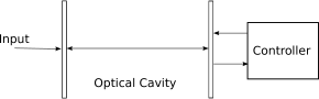
Figure 3: Quantum Plant: we wish to minimize the expected number of photons in the cavity.

Our plant is of the form (19) with

$$A = {}-\frac{\gamma}{2}I_{2\times 2};$$

$$B_{u} = -\sqrt{\kappa_{2}}I_{2\times 2};$$

$$B_{w_{1}} = \sqrt{\kappa_{1}}I_{2\times 2};$$

$$C = \sqrt{\kappa_{2}}I_{2\times 2};$$

$$D_{u} = I_{2\times 2};$$

$$D_{w_{1}} = 0_{2\times 2};$$

$$S_{w_{1}} = (1+2k_{n})I_{2\times 2}$$

$$\gamma = 0.2;$$

$$\kappa_{1} = 0.1;$$

$$\kappa_{2} = 0.1.$$ (27)

It is sufficient to minimize the cost function (20) with $R_{1}=I_{2\times 2}$ and $R_{2}=0_{2\times 2}$. Then $N=\frac{1}{4}J-0.5$.

Remark 6

We use $R_{2}=10^{-6}I_{2\times 2}$ to design both the heterodyne classical LQG controller and the auxiliary LQG controller. However, the cost function (20) for the resulting controller is then evaluated using $R_{2}=0_{2\times 2}$.

VI-A No Control

We first consider the case of no control as a reference. Here, the system input is driven by vacuum noise: $\,\mathrm{d}u=\,\mathrm{d}v_{1}$. The resulting closed loop system is:

$$\,\mathrm{d}x=Ax\,\mathrm{d}t+\begin{bmatrix}B_{w_{1}}&B_{u}\end{bmatrix}\begin{bmatrix}\,\mathrm{d}w_{1}\\ \,\mathrm{d}v_{1}\end{bmatrix},$$

where $\,\mathrm{d}w_{CL}=\left[\begin{smallmatrix}\,\mathrm{d}w_{1}\\ \,\mathrm{d}v_{1}\end{smallmatrix}\right]$ is a quantum Wiener process with covariance

$$S_{w_{CL}}=\begin{bmatrix}(1+2k_{n})I_{2\times 2}&0\\ 0&I_{2\times 2}\end{bmatrix}.$$

Equation (22) can then be used to find the value of the cost function (20) for a range of values for $k_{n}$.

VI-B Heterodyne measurement and classical LQG control

Next we consider combining heterodyne measurement with a classical optimal LQG controller. Heterodyne measurement introduces an additional vacuum noise input. Similarly, the output of the classical controller will contain a vacuum noise component when applied to the input of the plant. This is accounted for by making the following substitutions:

$$\,\mathrm{d}u = \,\mathrm{d}\tilde{u}+\,\mathrm{d}w_{3};$$

$$\,\mathrm{d}\tilde{y} = \,\mathrm{d}y+\,\mathrm{d}w_{2};$$

into (19) to obtain an augmented plant. Here $\,\mathrm{d}\tilde{u}$ and $\,\mathrm{d}\tilde{y}$ are classical signals which represent the input and output of the augmented plant. The resulting equations for the augmented plant are as follows:

$$\,\mathrm{d}x = Ax\,\mathrm{d}t+B_{u}\,\mathrm{d}\tilde{u}+B_{\tilde{w}}\,\mathrm{d}\tilde{w};$$

$$\,\mathrm{d}\tilde{y} = Cx\,\mathrm{d}t+D_{u}\,\mathrm{d}\tilde{u}+D_{\tilde{w}}\,\mathrm{d}\tilde{w}.$$

Here $A$, $B_{u}$, $C$, and $D_{u}$ are as before, and

$$B_{\tilde{w}} = \begin{bmatrix}{}-\sqrt{\kappa_{1}}I_{2\times 2}&0_{2\times 2}&{}-\sqrt{\kappa_{2}}I_{2\times 2}\end{bmatrix};$$

$$D_{\tilde{w}} = \begin{bmatrix}0_{2\times 2}&I_{2\times 2}&I_{2\times 2}\end{bmatrix};$$

$$\,\mathrm{d}\tilde{w} = \begin{bmatrix}\,\mathrm{d}w_{1}\\ \,\mathrm{d}w_{2}\\ \,\mathrm{d}w_{3}\end{bmatrix};$$

$$S_{\tilde{w}} = \begin{bmatrix}(1+2k_{n})I_{2\times 2}&0&0\\ 0&I_{2\times 2}&0\\ 0&0&I_{2\times 2}\end{bmatrix}.$$

As with the auxiliary LQG problem in our design algorithm, we treat $\,\mathrm{d}\tilde{w}$ as a standard classical Wiener process with intensity matrix $S_{\tilde{w}}$. We now have a standard classical LQG problem. We wish to find a controller of the form:

$$\,\mathrm{d}x_{K} = A_{K}x_{K}\,\mathrm{d}t+B_{y}\,\mathrm{d}\tilde{y};$$

$$\,\mathrm{d}\tilde{u} = C_{K}x_{K}\,\mathrm{d}t.$$

The estimator gain $K$ and the regulator gain $F$ are obtained in the usual manner. For this example $R_{2}=0_{2\times 2}$ but for computational reasons we assume $R_{2}$ takes a small value of $R_{2}=10^{-6}$ and hence $\left\{A_{K},B_{y},C_{K}\right\}$ are obtained. The closed loop system is then as follows:

$$\begin{bmatrix}\,\mathrm{d}x\\ \,\mathrm{d}x_{K}\end{bmatrix} = \mathcal{A}\begin{bmatrix}x\\ x_{K}\end{bmatrix}\,\mathrm{d}t+\mathcal{B}\,\mathrm{d}\tilde{w};$$

$$\mathcal{A} = \begin{bmatrix}A&B_{u}C_{K}\\ B_{y}C&A_{K}+B_{y}D_{u}C_{K}\end{bmatrix};$$

$$\mathcal{B} = \begin{bmatrix}B_{\tilde{w}}\\ B_{y}D_{\tilde{w}}\end{bmatrix}.$$

The value of the cost function (20) can now be calculated using (22) with $R_{2}=0_{2\times 2}$ and substituting $S_{\tilde{w}}$ for $S_{w_{CL}}$.

VI-C Quantum LQG control

Finally we consider our proposed control scheme. First the auxiliary LQG problem is formed. The auxiliary plant is given by (23) with parameters as in (27). The cost function is given by (25) with $R_{1}=I_{2\times 2}$ and $R_{2}=10^{-6}$.

Then, optimizing $J$ over $\rho$, we do the following:

1. Solve the auxiliary LQG problem as detailed above to obtain $\left\{A_{K},B_{y},C_{K}\right\}$.

2. Obtain a physically realizable quantum implementation of $\left\{A_{K},B_{y},C_{K}\right\}$. We do this by first attempting to apply Theorem 3 to obtain $B_{K1}$. If the conditions of this theorem are not met we apply Theorem 2 to obtain $B_{K1}$ and $B_{K2}$.

3. Evaluate the cost function (20) using (22) with $R_{1}=I_{2\times 2}$ and $R_{2}=0_{2\times 2}$.

VI-D Comparison of controller performance

The relative performance of the no control case, the classical LQG case and our coherent control case are illustrated in Figure 4 and Figure 5. In the regime where both the thermal noise driving the system and the quantum noises are significant, the coherent quantum feedback controller offers the best performance of the schemes considered. If we leave the quantum regime with $k_{n}\gg 0$, the relative performance benefits of the coherent quantum feedback controller over the measurement based feedback controller diminish as the thermal noise dominates the system and the quantum noises become insignificant by comparison. In the limit as $k_{n}\to 0$, where the system is driven only by vacuum noise, our proposed controller offers no advantage over the no control case. This is consistent with the idea that the cavity cannot be driven below the vacuum state.

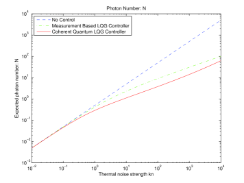
Figure 4: Expected photon number $N$ for no control, heterodyne measurement and classical LQG control, and coherent quantum LQG control.

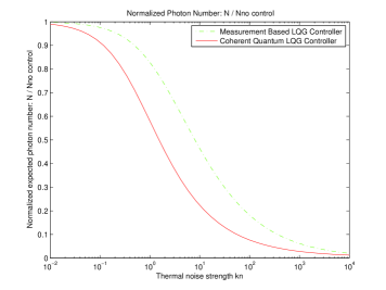
Figure 5: Normalized photon number $N/N_{NC}$ for heterodyne measurement and classical LQG control, and coherent quantum LQG control.

VII Conclusion

The notion of physical realizability is fundamental to the coherent quantum feedback control problem where we wish to implement a given synthesized controller as a quantum system. By introducing additional quantum noises, it is always possible to make a given LTI system physically realizable. However, introducing additional quantum noises is undesirable in terms of the control system performance. In this paper, we have given an expression for the number of introduced quantum noises that are necessary to make a given LTI system physically realizable. Our result also gives a method for constructing the resulting fully quantum system.

We also considered the case where a strictly proper transfer function is to be physically realized. We have given a result in terms of a Riccati equation for when it is possible to physically realize a specified transfer function by only introducing direct feedthrough vacuum noises and no additional quantum noises. We have also given conditions for when this Riccati equation has a suitable solution.

Using these results we have developed an algorithm for obtaining a suboptimal solution to a coherent quantum LQG control problem. Our example demonstrates the utility of our results and shows that coherent quantum feedback control can offer performance benefits over measurement based feedback control.

References

• [1] C. Gardiner and P. Zoller, Quantum Noise.   Berlin: Springer, 2000.
• [2] G. Auletta, M. Fortunato, and G. Parisi, Quantum Mechanics, ser. Quantum Mechanics.   Cambridge University Press, 2009.
• [3] M. R. James, H. I. Nurdin, and I. R. Petersen, “${H}^{\infty}$ control of linear quantum stochastic systems,” IEEE Transactions on Automatic Control, vol. 53, no. 8, pp. 1787–1803, 2008.
• [4] A. J. Shaiju and I. R. Petersen, “A frequency domain condition for the physical realizability of linear quantum systems,” IEEE Transactions on Automatic Control, vol. 57, no. 8, pp. 2033–2044, 2012.
• [5] H. I. Nurdin, M. R. James, and I. R. Petersen, “Coherent quantum LQG control,” Automatica, vol. 45, no. 8, pp. 1837–1846, 2009.
• [6] H. M. Wiseman and G. J. Milburn, Quantum Measurement and Control.   Cambridge University Press, 2010.
• [7] R. Vijay, C. Macklin, D. H. Slichter, S. J. Weber, K. W. Murch, R. Naik, A. N. Korotkov, and I. Siddiqi, “Stabilizing Rabi oscillations in a superconducting qubit using quantum feedback,” Nature, vol. 490, pp. 77–80, 2012.
• [8] A. I. Maalouf and I. R. Petersen, “Coherent ${H}^{\infty}$ control for a class of linear complex quantum systems,” IEEE Transactions on Automatic Control, vol. 56, no. 2, pp. 309–319, 2011.
• [9] H. Mabuchi, “Coherent-feedback quantum control with a dynamic compensator,” Physical Review A, vol. 78, p. 032323, 2008.
• [10] A. I. Maalouf and I. R. Petersen, “Bounded real properties for a class of linear complex quantum systems,” IEEE Transactions on Automatic Control, vol. 56, no. 4, pp. 786 – 801, 2011.
• [11] S. L. Vuglar and I. R. Petersen, “Singular perturbation approximations for general linear quantum systems,” in Proceedings of the Australian Control Conference, Sydney, Australia, Nov 2012, pp. 459–463, arXiv:1208.6155 [quant-ph].
• [12] H. I. Nurdin, M. R. James, and A. C. Doherty, “Network synthesis of linear dynamical quantum stochastic systems,” SIAM Journal on Control and Optimization, vol. 48, no. 4, pp. 2686–2718, 2009.
• [13] H. Nurdin, “Synthesis of linear quantum stochastic systems via quantum feedback networks,” IEEE Transactions on Automatic Control, vol. 55, no. 4, pp. 1008 –1013, April 2010.
• [14] ——, “On synthesis of linear quantum stochastic systems by pure cascading,” IEEE Transactions on Automatic Control, vol. 55, no. 10, pp. 2439 –2444, October 2010.
• [15] I. R. Petersen, “Cascade cavity realization for a class of complex transfer functions arising in coherent quantum feedback control,” Automatica, vol. 47, no. 8, pp. 1757 – 1763, 2011.
• [16] S. L. Vuglar and I. R. Petersen, “How many quantum noises need to be added to make an LTI system physically realizable?” in Proceedings of the Australian Control Conference, Melbourne, Australia, November 2011.
• [17] ——, “A numerical condition for the physical realizability of a quantum linear system,” in Proceedings of the 20th International Symposium on Mathematical Theory of Networks and Systems, Melbourne, Australia, 2012.
• [18] ——, “Quantum implemention of an LTI System with the minimal number of additional quantum noise inputs.” in Proceedings of the 12th biannual European Control Conference, Zurich, Switzerland, 2013, arXiv:1304.6815 [quant-ph].
• [19] R. A. Horn and C. R. Johnson, Matrix Analysis.   Cambridge, UK: Cambridge University Press, 1985.
• [20] D. S. Bernstein, Matrix Mathematics: Theory, Facts, And Formulas with Application to Linear Systems Theory.   Princeton, New Jersey: Princeton University Press, 2005.
• [21] A. Baker, Matrix Groups: An Introduction to Lie Group Theory.   New York: Springer-Verlag, 2002.
• [22] K. Zhou, J. Doyle, and K. Glover, Robust and Optimal Control.   Upper Saddle River, NJ: Prentice-Hall, 1996.
• [23] H. Kwakernaak and R. Sivan, Linear Optimal Control Systems.   Wiley, 1972.
• [24] R. Hamerly and H. Mabuchi, “Coherent controllers for optical-feedback cooling of quantum oscillators,” Phys. Rev. A, vol. 87, no. 1, p. 013815, 2013.