Theory of angular dispersive imaging hard x-ray spectrographs

Abstract

A spectrograph is an optical instrument that disperses photons of different energies into distinct directions and space locations, and images photon spectra on a position-sensitive detector. Spectrographs consist of collimating, angular dispersive, and focusing optical elements. Bragg reflecting crystals arranged in an asymmetric scattering geometry are used as the dispersing elements. A ray-transfer matrix technique is applied to propagate x-rays through the optical elements. Several optical designs of hard x-ray spectrographs are proposed and their performance is analyzed. Spectrographs with an energy resolution of 0.1 meV and a spectral window of imaging up to a few tens of meVs are shown to be feasible for inelastic x-ray scattering (IXS) spectroscopy applications. In another example, a spectrograph with a 1-meV spectral resolution and $85$-meV spectral window of imaging is considered for Cu K-edge resonant IXS (RIXS).

I Introduction

Ultra-fast dynamics in condensed matter in a picosecond (ps) to a 100-ps regime on atomic- to meso-scales is still inaccessible for studies using any known experimental probe. A gap remains in experimental capabilities between the low-frequency (visible and ultraviolet light) and high-frequency (x-rays and neutrons) inelastic scattering techniques. Figure 1 shows how the time-length space or the relevant energy-momentum space of excitations in condensed matter is accessed by different inelastic scattering probes: neutron (INS), x-ray (IXS), ultraviolet (IUVS), and Brillouin (BLS); as well as how the remaining gap could be closed by enhancing inelastic x-ray scattering capabilities. Ultra-high-resolution IXS (UHRIXS) has the potential to enter the unexplored dynamic range of excitations in condensed matter. This would, however, require achieving a very high spectral resolution on the order of 0.1 meV, and momentum transfer resolution around 0.01 nm^-1 (light green area in Fig. 1). In approaching this goal, a novel IXS spectrometer has been demonstrated recently Shvyd’ko et al. (2014); the spectral resolution improved from 1.5 meV to 0.6 meV, the momentum transfer resolution improved from 1 nm^-1 to 0.25 nm^-1 (dark-green and green areas in Fig. 1, respectively), and the spectral contrast improved by an order of magnitude compared to the traditional IXS spectrometers Burkel et al. (1987); Sette et al. (1995); Masciovecchio et al. (1996); Baron et al. (2001); Sinn et al. (2001); Said et al. (2011). The gap became narrower, but did not close.

Figure 1: (Color online) Time-length ($t-\lambda$) and relevant energy-momentum ($\varepsilon\!-\!Q$) space of excitations in condensed matter and how it is accessed by different inelastic scattering probes: neutron (INS), x-ray (IXS), ultraviolet (IUVS), and Brillouin (BLS). The ultra-high-resolution IXS spectrometer presented in Ref. Shvyd’ko et al. (2014) entered the previously inaccessible region marked in green. The novel capabilities discussed in the present paper will enable IXS experiments with even higher resolution, 0.1-meV and 0.01-nm^-1, in the region marked in light green, and will close completely the existing gap between the high-frequency and low-frequency probes. The energy $\varepsilon=E_{{}_{\mathrm{f}}}\!-\!E_{{}_{\mathrm{i}}}$ and the momentum $\mbox{\boldmath$Q$}=\mbox{\boldmath$k$}_{{}_{\mathrm{f}}}\!-\!\mbox{\boldmath$k$}_{{}_{\mathrm{i}}}$ transfers from initial to final photon/neutron states are measured in inelastic scattering experiments, schematically shown in the oval inset.

The outstanding problems in the condensed matter physics, such as the nature of the liquid to glass transitions, have yet to be fully addressed. Here we propose an approach of how this problem could be solved, and how UHRIXS spectrometers could become efficient imaging optical devices. This approach is a further development of the proposal presented in Shvyd’ko (2011, 2012); Shvyd’ko et al. (2013a).

Figure 2: (Color online) Scheme of the Czerny-Turner type spectrograph Czerny and Turner (1930) with (a) a diffraction grating, or (b) a crystal in asymmetric x-ray Bragg diffraction as dispersing element (DE). Other components include radiation source S, collimating and focusing mirrors M${}_{{}_{\mathrm{C}}}$ and M${}_{{}_{\mathrm{F}}}$, and position sensitive detector Det. (c) Multi-crystal multi-reflection CDDW optic, an example of a hard x-ray “diffraction grating” (DE element) with enhanced dispersion rate, suitable for hard x-ray spectrographs Shvyd’ko et al. (2013a).

In a typical IXS experiment Sinn (2001), x-rays incident on a sample are monochromatized to a very small bandwidth corresponding to a desired energy resolution. The spectral analysis of photons scattered from a sample is performed by an x-ray analyzer, featuring the same spectral bandwidth and acting like a spectral slit. Monochromatization from approximately a $100$-eV to a $1$-meV bandwidth results in a dramatic reduction of the photon flux generated by undulator sources at synchrotron radiation facilities, typically by more than five orders of magnitude. The angular acceptance, $1-10$ mrad, of the analyzer is much large than the angular acceptance, $10-20~{}\mu$rad, of the monochromator; however, it is still orders of magnitude smaller than the total solid angle of scattering by the sample. It is also much smaller than the $10-100$-meV window desired for the spectral analysis. All this results in very small countrates $10-0.01$ Hz in IXS experiments Sinn (2001). Further improvements to the 0.1-meV resolution using such an approach would only result in yet another substantial reduction of the countrate and time-consuming experiments.

A possible solution to this problem would be to create a spectrometer that would not only feature the high spectral resolution, but would also be capable of imaging x-ray spectra in a broad spectral window. We will refer to such optical devices as x-ray spectrographs.

Czerny-Turner type spectrographs Czerny and Turner (1930) are now standard in infrared, visible, and ultraviolet spectroscopies Shafer et al. (1964); Lee et al. (2010). In its classical arrangement, a spectrograph is comprised of four elements [see Fig. 2(a)]: (1) a collimating mirror, M${}_{{}_{\mathrm{C}}}$, that collects photons from a radiation source, S, and collimates the photon beam; (2) a dispersing element, DE, such as a diffraction grating or a prism, which scatters photons of different energies into different directions $\theta^{\prime}(E)$ due to angular dispersion; (3) a curved mirror, M${}_{{}_{\mathrm{F}}}$, that focuses photons of different energies into different locations $x(E)$ due to linear dispersion; and (4) a spatially sensitive detector, Det, placed in the focal plane to record the whole photon spectrum.

The feasibility of hard x-ray angular-dispersive spectrographs of the Czerny-Turner type has been discussed in Shvyd’ko (2011, 2012); Shvyd’ko et al. (2013a). A hard x-ray equivalent of the diffraction grating is a Bragg diffracting crystal with diffracting atomic planes at an asymmetry angle $\eta\not=0$ to the entrance crystal surface [see Fig. 2(b)] Matsushita and Kaminaga (1980a); Brauer et al. (1995); Shvyd’ko (2004). Angular dispersion rates attainable in a single Bragg reflection are typically small, ${\mathcal{D}}\simeq 8~{}\mu$rad/meV Shvyd’ko et al. (2006, 2011), and are the main obstacle to realizing hard x-ray spectrographs. The angular dispersion rate can be enhanced dramatically, by almost two orders of magnitude, by successive asymmetric Bragg reflections compared to that in a single Bragg reflection Shvyd’ko et al. (2013a). An enhanced angular dispersion rate in multi-crystal arrangements is crucial for the feasibility of hard x-ray angular-dispersive spectrographs. An x-ray angular-dispersive spectrograph was demonstrated experimentally in Shvyd’ko et al. (2013a), using the so-called multi-crystal collimation-dispersion-wavelength-selection (CDW) optic , achieving spectral resolution of better than $100~{}\mu$eV with 9.1 keV x-ray photons. However, the spectral window in which the CDW optic permitted imaging x-ray spectra was small, about $450~{}\mu$eV. Increasing the spectral window of ultra-high-resolution x-ray spectrographs, is extremely important.

In pursuing this goal, and in seeking solutions to this problem, a theory of hard x-ray spectrographs is developed here. In Section II, a ray-transfer matrix technique Kogelnik and Li (1966); Matsushita and Kaminaga (1980a, b); Siegman (1986); Hodgson and Weber (2005); Smilgies (2008) is applied to propagate x-rays through complex optical x-ray systems in the paraxial approximation. The following systems are considered: successive Bragg reflections from crystals (Section  II.4), focusing system (Section II.5), focusing monochromators (Section II.6), and finally Czerny-Turner-type spectrographs (Section II.7). Solutions for broadband hard x-ray imaging spectrographs are considered in Section III. Several “diffraction grating” designs for hard x-ray spectrographs are proposed to ensure a high energy resolution, broad spectral window of imaging, and large angular acceptance. Spectrographs with an energy resolution of $\Delta E=0.1$ meV and a spectral window of imaging up to $\Delta E_{{}_{\cup}}=45$ meV are shown to be feasible for IXS applications in Section III.1 and Section III.2.1. In Section III.2.2, a spectrograph with a 1-meV spectral resolution and 85-meV spectral imaging window is considered for Cu K-edge resonant IXS (RIXS) applications.

II Ray-Transfer Matrices of X-ray Optical Systems and Spectrographs

The main goal of this article is to develop a theory of Czerny-Turner-type hard x-ray spectrographs. The conceptual optical scheme of the Czerny-Turner-type spectrographs is presented in Fig. 2(a). In the hard x-ray regime, the role of the diffraction grating is played by a single crystal in asymmetric Bragg diffraction scattering geometry, as shown in Fig. 2(b), or by an arrangement of several single crystals. One possible example of multi-crystal arrangements discussed in Shvyd’ko et al. (2013a), although is not the only possibility, is shown in Fig. 2(c). The purpose of the theory is to calculate the spectral resolution and other performance characteristics of hard x-ray spectrographs, and their dependence on physical parameters of constituent optical elements.

In approaching the main goal, we consider optical systems starting with simple ones, such as a focusing element and Bragg reflection from a crystal, and proceed to more complex systems, such as successive Bragg reflections from multiple crystals, focusing systems, focusing monochromators, and finally spectrographs.

II.1 Ray transfer matrix technique

We will use a ray-transfer matrix technique Kogelnik and Li (1966); Matsushita and Kaminaga (1980a, b); Siegman (1986); Hodgson and Weber (2005); Smilgies (2008) to propagate paraxial x-rays through optical structures. In a standard treatment, a paraxial ray in a particular reference plane of an optical system (the plane perpendicular to the optical axis $z$) is characterized by its distance $x$ from the optical axis and by its angle or slope $\xi$ with respect to that axis. The ray is presented by a two-dimensional vector $\mbox{\boldmath$r$}=(x,\xi)$. Interactions with optical elements are described by $2\times 2$ dimensional $\{AB;CD\}$ matrices. The ray vector $\mbox{\boldmath$r$}_{{}_{1}}=(x_{{}_{1}},\xi_{{}_{1}})$ at an input reference plane (source plane) is transformed to $\mbox{\boldmath$r$}_{{}_{2}}=\hat{O}\mbox{\boldmath$r$}_{{}_{1}}$ at the output reference plane (image plane), where $\hat{O}$ is the “ABCD” matrix of an element placed between the reference planes.

Angular dispersion in Bragg reflection from asymmetrically cut crystals results in deviation of the beam from the unperturbed optical axis due to a change, $\delta E$, in the photon energy from $E$ to $E+\delta E$ Matsushita and Kaminaga (1980a); Brauer et al. (1995); Shvyd’ko (2004). This causes “misalignment” of the paraxial optical system, which can be conveniently described by a $3\times 3$ $\{ABG;CDF;001\}$ matrix by adding additional coordinate $\delta E$ to vector $\mbox{\boldmath$r$}=(x,\xi,\delta E)$ Matsushita and Kaminaga (1980a, b); Siegman (1986); Martínez (1988); Smilgies (2008).

Table 1 presents ray-transfer matrices used in this paper. In the first three rows, 1–3, matrices are given for simple elements of the spectrograph, such as propagation in free space, thin lens or focusing mirror, and Bragg reflection from a crystal. In the following rows ray-transfer matrices are shown for arrangements composed of several optical elements, such as successive multiple Bragg reflections from several crystals, rows 4–5; focusing system, row 6; focusing monochromators, rows 7–8; and finally spectrographs, row 9, on which the paper is focused. The matrices of the multi-element systems are obtained by successive multiplication of the matrices of the constituent optical elements.

II.2 Bragg reflection and reference system

All the ray-transfer matrices are presented in the right-handed coordinate system $\{x,y,z\}$ with the $\hat{\mbox{\boldmath$z$}}$-axis looking in the direction of the optical axis both before and after each optical element, as illustrated in Fig. 3 on an example of a Bragg reflecting crystal. This absolute reference system is retained through all interactions with all optical elements. We use the convention that positive is the counterclockwise sense of angular variations $\xi$ of the ray slope in the $(x,z)$ plane. For Bragg reflections, $\xi_{{}_{1}}$ is understood as a small angular deviation from a nominal glancing angle of incidence $\theta$ to the reflecting atomic planes of the crystal; $\xi_{{}_{2}}$ is understood as a small angular deviation from the nominal glancing angle of reflection $\theta^{\prime}$. The angles $\theta$ and $\theta^{\prime}$ define the optical axis. The angle $\theta$ is determined by Bragg’s law $2K\sin\theta=H$, while $\theta^{\prime}$ is determined by the relationship Kuriyama and Boettinger (1976)

$$\cos(\theta^{\prime}-\eta)=\cos(\theta+\eta)+\frac{H}{K}\sin{\eta}.$$ (1)

Equation (1) is a consequence, first, of the conservation of the tangential components $(\mbox{\boldmath$K$}_{{}_{H}})_{t}=(\mbox{\boldmath$K$}_{{}_{0}}+\mbox{\boldmath$H$})_{t}$ with respect to the entrance crystal surface for the momentum, $\mbox{\boldmath$K$}_{{}_{0}}$, of the incident x-ray photon and the momentum, $\mbox{\boldmath$K$}_{{}_{H}}$, of the photon Bragg reflected from the crystal with a diffraction vector $H$ [see Fig. 2(b)]. It is also a consequence of the conservation of the photon energies $|\mbox{\boldmath$K$}_{{}_{H}}|\hbar c=|\mbox{\boldmath$K$}_{{}_{0}}|\hbar c=K\hbar c=E$. The reflecting atomic planes are at an asymmetry angle, $\eta$, to the entrance crystal surface. The asymmetry angle, $\eta$, is defined here to be positive in the geometry shown in Figs. 3(a) and 3(b), and negative in the geometry with reversed incident and reflected x-rays (not shown).

Optical system	Matrix notation	Ray-transfer matrix	Definitions and Remarks
Free space Kogelnik and Li (1966); Hodgson and Weber (2005); Siegman (1986) (1)	$\hat{P}(l)$	$\left(\begin{array}[]{ccc}1&l&0\\ 0&1&0\\ 0&0&1\end{array}\right)$	$l$ – distance
Thin lens Kogelnik and Li (1966); Hodgson and Weber (2005); Siegman (1986) (2)	$\hat{L}(f)$	$\left(\begin{array}[]{ccc}1&0&0\\ -\frac{1}{f}&1&0\\ 0&0&1\end{array}\right)$	$f$ – focal length
Bragg reflection from a crystal Matsushita and Kaminaga (1980a, b) (3)	$\hat{C}(b,s{\mathcal{D}})$	$\left(\begin{array}[]{ccc}{1}/{b}&0&0\\ 0&b&s{\mathcal{D}}\\ 0&0&1\end{array}\right)$	$b=-\frac{\sin(\theta+\eta)}{\sin(\theta-\eta)}$ asymmetry factor; ${\mathcal{D}}=-(1/E)(1+b)\tan\theta$ angular dispersion rate; $s=-1$ for clockwise, and $s=+1$ counterclockwise ray deflection.
Successive Bragg reflections $\hat{C}(\!b_{{}_{n}},s_{{}_{n}}{\mathcal{D}}_{{}_{n}}\!)\dotsb\hat{C}(\!b_{{}_{1}},s_{{}_{1}}{\mathcal{D}}_{{}_{1}}\!)$ (4)	$\hat{C}(b_{\cup_{{}_{n}}},{\mathcal{D}}_{\cup_{{}_{n}}})$	$\left(\begin{array}[]{ccc}1/b_{\cup_{{}_{n}}}&0&0\\ 0&b_{\cup_{{}_{n}}}&{\mathcal{D}}_{\cup_{{}_{n}}}\\ 0&0&1\end{array}\right)$	$b_{\cup_{{}_{n}}}=b_{{}_{1}}b_{{}_{2}}b_{{}_{3}}\dotsc b_{{}_{n}}$ ${\mathcal{D}}_{\cup_{{}_{n}}}=b_{{}_{n}}{\mathcal{D}}_{\cup_{{}_{n-1}}}+s_{{}_{n}}{\mathcal{D}}_{{}_{n}}$ $s_{i}=\pm 1$, $i=1,2,...,n$
Successive Bragg reflections with space between crystals $\hat{C}(\!b_{{}_{n}},s_{{}_{n}}{\mathcal{D}}_{{}_{n}}\!)\dotsb\hat{P}(\!l_{{}_{12}}\!)\hat{C}(\!b_{{}_{1}},s_{{}_{1}}{\mathcal{D}}_{{}_{1}}\!)$ (5)	$\hat{K}(b_{\cup_{{}_{n}}},{\mathcal{D}}_{\cup_{{}_{n}}},l)$	$\left(\begin{array}[]{ccc}1/b_{\cup_{{}_{n}}}&B_{\cup_{{}_{n}}}&G_{\cup_{{}_{n}}}\\ 0&b_{\cup_{{}_{n}}}&{\mathcal{D}}_{\cup_{{}_{n}}}\\ 0&0&1\end{array}\right)$	$B_{\cup_{{}_{n}}}\!=\!\frac{B_{\cup_{{}_{n-1}}}+b_{\cup_{{}_{n-1}}}l_{{}_{n-1n}}}{b_{{}_{n}}}$ $G_{\cup_{{}_{n}}}\!=\!\frac{G_{\cup_{{}_{n-1}}}+{\mathcal{D}}_{\cup_{{}_{n-1}}}l_{{}_{n-1n}}}{b_{{}_{n}}}$ $B_{\cup_{{}_{1}}}\!=\!0,\hskip 14.22636ptG_{\cup_{{}_{1}}}\!=\!0$
Focusing system $\hat{P}(l_{{}_{2}})\hat{L}(f)\hat{P}(l_{{}_{1}})$ (6)	$\hat{F}(l_{{}_{2}},f,l_{{}_{1}})$	$\left(\begin{array}[]{ccc}1-\frac{l_{{}_{2}}}{f}&B_{{}_{\mathrm{F}}}&0\\ -\frac{1}{f}&1-\frac{l_{{}_{1}}}{f}&0\\ 0&0&1\end{array}\right)$	$B_{{}_{\mathrm{F}}}=l_{{}_{1}}l_{{}_{2}}\left(\frac{1}{l_{{}_{1}}}+\frac{1}{l_{{}_{2}}}-\frac{1}{f}\right)$
Focusing monochromator I Kohn et al. (2009) $\hat{P}(l_{{}_{3}})\hat{C}(b_{\cup_{{}_{n}}}\!,{\mathcal{D}}_{\cup_{{}_{n}}}\!)\hat{F}(l_{{}_{2}},f,l_{{}_{1}})$ (7)	$\hat{M_{{}_{\mathrm{I}}}}(l_{{}_{3}},b_{\cup_{{}_{n}}}\!,{\mathcal{D}}_{\cup_{{}_{n}}}\!,l_{{}_{2}},f,l_{{}_{1}})$	$\left(\!\!\begin{array}[]{ccc}\frac{1}{b_{\cup_{{}_{n}}}}\!\left(\!1\!-\!\frac{l_{{}_{23}}}{f}\!\right)&B_{{}_{\mathrm{I}}}&l_{{}_{3}}{\mathcal{D}}_{\cup_{{}_{n}}}\\ -\frac{b_{\cup_{{}_{n}}}}{f}&b_{\cup_{{}_{n}}}\!\left(\!1\!-\!\frac{l_{{}_{1}}}{f}\!\right)&{\mathcal{D}}_{\cup_{{}_{n}}}\\ 0&0&1\end{array}\!\!\right)$	$B_{{}_{\mathrm{I}}}=\frac{l_{{}_{1}}l_{{}_{23}}}{b_{\cup_{{}_{n}}}}\!\left(\!\frac{1}{l_{{}_{1}}}\!+\!\frac{1}{l_{{}_{23}}}\!-\!\frac{1}{f}\!\right)$ $l_{{}_{23}}=l_{{}_{2}}+b_{\cup_{{}_{n}}}^{2}l_{{}_{3}}$
Focusing monochromator II $\hat{F}(l_{{}_{3}},f,l_{{}_{2}})\hat{C}(b_{\cup_{{}_{n}}}\!,{\mathcal{D}}_{\cup_{{}_{n}}}\!)\hat{P}(l_{{}_{1}})$ (8)	$\hat{M_{{}_{\mathrm{II}}}}(l_{{}_{3}},f,l_{{}_{2}},b_{\cup_{{}_{n}}}\!,{\mathcal{D}}_{\cup_{{}_{n}}}\!,l_{{}_{1}})$	$\left(\!\!\begin{array}[]{ccc}\frac{1}{b_{\cup_{{}_{n}}}\!}\!\left(\!1\!-\!\frac{l_{{}_{3}}}{f}\!\right)&B_{{}_{\mathrm{II}}}&X{\mathcal{D}}_{\cup_{{}_{n}}}\\ -\frac{1}{fb_{\cup_{{}_{n}}}}&b_{\cup_{{}_{n}}}\!\!\left(\!1\!-\!\frac{l_{12}}{f}\!\right)&\left(\!1\!-\!\frac{l_{{}_{2}}}{f}\!\right)\!{\mathcal{D}}_{\cup_{{}_{n}}}\\ 0&0&1\end{array}\!\!\right)$	$B_{{}_{\mathrm{II}}}\!=\!b_{\cup_{{}_{n}}}\!l_{{}_{12}}l_{{}_{3}}\!\left(\!\frac{1}{l_{{}_{12}}}\!+\!\frac{1}{l_{{}_{3}}}\!-\!\frac{1}{f}\!\right)$ $l_{{}_{12}}=l_{{}_{1}}/b_{\cup_{{}_{n}}}^{2}+l_{{}_{2}}$ $X=l_{{}_{2}}+l_{{}_{3}}-l_{{}_{2}}l_{{}_{3}}/f$ $B_{{}_{\mathrm{II}}}\!=\!0\Rightarrow X\!=\!l_{{}_{3}}l_{{}_{1}}\!/(\!b_{\cup_{{}_{n}}}^{2}\!l_{{}_{12}}\!)$
Spectrograph $\hat{F}(\!f_{{}_{2}}\!,\!f_{{}_{2}}\!,\!l_{{}_{2}}\!)\hat{C}(\!b_{\cup_{{}_{n}}}\!,\!{\mathcal{D}}_{\cup_{{}_{n}}}\!)\hat{F}(\!l_{{}_{1}}\!,\!f_{{}_{1}}\!,\!f_{{}_{1}}\!)$ (9)	$\hat{S}(f_{{}_{2}},l_{{}_{2}},b_{\cup_{{}_{n}}}\!,{\mathcal{D}}_{\cup_{{}_{n}}}\!,l_{{}_{1}},f_{{}_{1}})$	$\left(\!\!\begin{array}[]{ccc}-\frac{b_{\cup_{{}_{n}}}f_{{}_{2}}\!}{f_{{}_{1}}\!}&0&f_{{}_{2}}{\mathcal{D}}_{\cup_{{}_{n}}}\\ \frac{(\!l_{{}_{1}}\!-\!f_{{}_{1}}\!)\!+\!(\!l_{{}_{2}}\!-\!f_{{}_{2}}\!)b_{\cup_{{}_{n}}}^{2}\!}{\!b_{\cup_{{}_{n}}}f_{{}_{1}}f_{{}_{2}}\!}&-\frac{f_{{}_{1}}}{b_{\cup_{{}_{n}}}\!f_{{}_{2}}}&\left(\!1\!-\!\frac{l_{{}_{2}}}{f_{{}_{2}}}\!\right)\!{\mathcal{D}}_{\cup_{{}_{n}}}\!\\ 0&0&1\end{array}\!\!\right)$

Table 1: Table of ray-transfer matrices $\{ABG,CDF,001\}$ used in the paper. The matrices for the focusing monochromators and the imaging spectrograph presented here are calculated with multi-crystal matrix $\hat{C}(b_{\cup_{{}_{n}}},{\mathcal{D}}_{\cup_{{}_{n}}})$ from row 4, assuming zero free space between crystals in successive Bragg reflections. Generalization to a more realistic case of nonzero distances between the crystals requires application of matrix $\hat{K}(b_{\cup_{{}_{n}}},{\mathcal{D}}_{\cup_{{}_{n}}},l)$ from row 5. The results are discussed in the text.

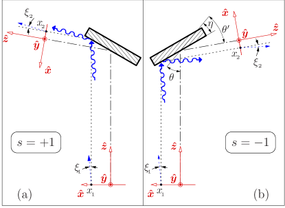
Figure 3: (Color online) Schematic elucidating the definition of an absolute right-handed coordinate system $\{x,y,z\}$ with the $\hat{\mbox{\boldmath$z$}}$-axis always looking in the direction of the optical axis (dash-dotted line) both before and after each optical element, a Bragg reflecting crystal in this particular case. By definition, positive is the counterclockwise sense of angular variations $\xi$ of ray slopes in the $(x,z)$ plane. Shown are examples of an optical element “Bragg reflection from a crystal” with (a) counterclockwise deflection, for which deflection sign $s=+1$; and (b) clockwise deflection of the reflected beam with $s=-1$. In the input reference system, the incident x-ray beam (wavy vector line) impinges onto the crystal at a glancing angle of incidence $\theta-s\xi_{{}_{1}}$ to the Bragg reflecting planes and with coordinate $x_{{}_{1}}$. It is reflected at a glancing angle of reflection $\theta^{\prime}+s\xi_{{}_{2}}$ with coordinate $x_{{}_{2}}$, as seen in the output reference system. Both $x$ and $\xi$ change signs upon reflection.

For the Bragg-reflection matrix $\{ABG,CDF,001\}$ the nonzero elements $A=1/D$, $D=\xi_{{}_{2}}/\xi_{{}_{1}}$, $F=\xi_{{}_{2}}/\delta E$ are calculated from Eq. (1) as follows :

$$D\,=\,b,\hskip 14.22636ptA\,=\,1/b,\hskip 14.22636ptb\,=\,-\frac{\sin(\theta+\eta)}{\sin(\theta-\eta)},$$ (2)

$$F\,=\,s\,{\mathcal{D}},\hskip 14.22636pt{\mathcal{D}}=\frac{2\sin\theta\sin{\eta}}{E\sin(\theta-\eta)}\equiv-\frac{1}{E}(1+b)\tan\theta,$$ (3)

by using the following variations: $\theta\rightarrow\theta-s\xi_{{}_{1}}$, $\theta^{\prime}\rightarrow\theta^{\prime}+s\xi_{{}_{2}}$, $E\rightarrow E+\delta E$ (see caption to Fig. 3). The angular dispersion rate ${\mathcal{D}}$ in Eq. (3) describes how the photon energy variation $\delta E$ changes the reflection angle at a fixed incidence angle. The deflection sign factor $s$ allows for the appropriate sign, depending on the scattering geometry. It is defined to be $s=+1$ if the Bragg reflection deflects the ray counterclockwise [Fig. 3(a)]. It is $s=-1$ if the reflected ray is deflected clockwise [Fig. 3(b)]. Asymmetry factor $b$ in Eq. (2) describes, in particular, how the beam size and beam divergence change upon Bragg reflection.

The ray transfer matrix for a Bragg reflection from a crystal presented in row 3 of Table 1 is equivalent to that introduced by Matsushita and Kaminaga Matsushita and Kaminaga (1980a, b), with the exception for different signs of the elements and the additional deflection sign factor $s$. Positive absolute values $|b|$ were used in local coordinate systems in Matsushita and Kaminaga (1980a, b). Here we use the absolute coordinate system to correctly describe transformations in multi-element optical arrangements. The choice of the absolute coordinate system is especially important to allow for inversion of the transverse coordinate and inversion of the slope when an optical ray is specularly reflected from a mirror or Bragg reflected from a crystal. Because of such inversion $x_{{}_{1}}$ and $x_{{}_{2}}$ as well as $\xi_{{}_{1}}$ and $\xi_{{}_{2}}$ have opposite signs, as shown in Figs. 3(a) and 3(b). A negative value of the asymmetry factor, $b$, in the Bragg reflection ray transfer matrix reflects this inversion upon each Bragg reflection.

The Bragg diffraction $\hat{C}(b,{\mathcal{D}})$ matrix is similar to the ray-transfer matrix of the diffraction grating (see, e.g., Martínez (1988)). The similarity is because both the asymmetry factor, $b$, and the angular dispersion rate, ${\mathcal{D}}$, are derived from Eq. (1), which coinsides with the well-know in optics grating equation. The magnification factor, $m$, used in the diffraction grating matrix is equivalent to $1/|b|$.

II.3 Thin lens or elliptical mirror

The ray-transfer matrix of a thin lens $\hat{L}(f)$ Kogelnik and Li (1966); Hodgson and Weber (2005); Siegman (1986) has a focal distance, $f$, as a parameter. Compound refractive lenses Snigirev et al. (1996) can be used for focusing and collimation in the hard x-ray regime, and described by such a matrix to a certain approximation. Alternatively, ellipsoidal total reflection mirrors could be applied, which transform radiation from a point source at one focal point to a point source located at the second focal point. The ray-transfer matrix of an ellipsoidal mirror has a structure identical to the ray-transfer matrix of a thin lens; however, $1/f=1/R_{{}_{1}}+1/R_{{}_{2}}$, where $R_{{}_{1}}$ and $R_{{}_{2}}$ are the distances from the center of the section of the ellipsoid employed to the foci of the generating ellipse Goldsmith (1998).

The basic ray matrices given in the first three rows of Table 1 can be combined to represent systems that are more complex.

II.4 Successive Bragg reflections

The ray-transfer matrix $\hat{C}_{\cup_{{}_{n}}}(b_{\cup_{{}_{n}}},{\mathcal{D}}_{\cup_{{}_{n}}})$ describing successive Bragg reflections from $n$ different crystals has a structure identical to that of the single Bragg reflection ray-transfer matrix $\hat{C}(b,{\mathcal{D}})$; however, the asymmetry factor, $b$, and the angular dispersion rate, ${\mathcal{D}}$, are substituted by the appropriate cumulative values $b_{\cup_{{}_{n}}}$, and ${\mathcal{D}}_{\cup_{{}_{n}}}$, respectively, as defined in row 4 of Table 1. The cumulative angular dispersion rate, ${\mathcal{D}}_{\cup_{{}_{n}}}$, derived in the present paper coincides with the expression first derived in Shvyd’ko et al. (2013a) using an alternative approach. It should be noted that the ray-transfer matrix $\hat{C}_{\cup_{n}}(b_{\cup_{{}_{n}}},{\mathcal{D}}_{\cup_{{}_{n}}})$ presented in Table 1, row 4, was derived neglecting propagation through free space between the crystals.

With nonzero distances $l_{{}_{i-1\ i}}$ between the crystals $i-1$ and $i$ ($i=2,3,...,n$) taken into account, the ray-transfer matrix of successive Bragg reflections changes to $\hat{K}_{\cup_{n}}(b_{\cup_{{}_{n}}},{\mathcal{D}}_{\cup_{{}_{n}}},l)$, as presented in row 5 of Table 1. Most of the elements of the modified ray-transfer matrix still remain unchanged, except for elements $B_{\cup_{{}_{n}}}$ and $G_{\cup_{{}_{n}}}$, which become nonzero. These elements are defined by recurrence relations in the table. Nonzero distances $l_{{}_{i-1\ i}}$ between the crystals result in an additional change $B_{\cup_{{}_{n}}}\xi$ of the linear size of the source image due to an angular spread $\xi$, and in an spatial transverse shift $G_{\cup_{{}_{n}}}\delta E$ of the image (linear dispersion) due to a spectral variation $\delta E$.

II.5 Focusing system

In the focusing system [see graph in row 6 of Table 1] a source in a reference source plane at a distance $l_{{}_{1}}$ downstream a lens or an elliptical mirror is imaged onto the reference image plane at a distance $l_{{}_{2}}$ upstream of the lens. The ray-transfer matrix of the focusing system is a product of the ray-transfer matrices of the free space $\hat{P}(l_{{}_{1}})$, the thin lens $\hat{L}(f)$, and another free space matrix $\hat{P}(l_{{}_{2}})$. If defined in Table 1 for the focusing system parameter $B_{{}_{\mathrm{F}}}=0$, the classical lens equation is valid:

$$\frac{1}{l_{{}_{1}}}+\frac{1}{l_{{}_{2}}}=\frac{1}{f}.$$ (4)

In this case, the system images the source with inversion and a magnification factor $1-l_{{}_{2}}/f=-l_{{}_{2}}/l_{{}_{1}}$ independent of the angular spread of rays in the source plane.

II.6 Focusing monochromators

Rows 7–8 in Table 1 present ray-transfer matrices of focusing monochromators, optical systems comprising a lens or an elliptical mirror, and an arrangement of crystals, respectively.

We will distinguish between two different types of focusing monochromators. If the lens is placed upstream of the crystal arrangement, we will refer to such optic as a focusing monochromator, I, presented in row 7 of Table 1. If the lens is placed downstream, this optic will be referred to as focusing monochromator, II, presented in row 8.

II.6.1 Focusing monochromator I

The focusing monochromator I with a single crystal was introduced in Kohn et al. (2009), and its performance was analyzed using the wave theory developed there. The ray-transfer matrix approach used in the present paper leads to similar results, except for diffraction effects being neglected here.

We consider here a general case with a multi-crystal arrangement. The ray-transfer matrix presented in Table 1 was derived neglecting propagation through free space between the crystals. The following expressions are valid for the elements of the ray-transfer matrix of the focusing monochromator I if nonzero distances between the crystals of the monochromator are taken into account:

$$\tilde{A}_{{}_{\mathrm{I}}}=\frac{1}{b_{\cup_{{}_{n}}}}\left(1-\frac{\tilde{l}_{{}_{23}}}{f}\right),$$ (5)

$$\tilde{l}_{{}_{23}}=l_{{}_{23}}+b_{\cup_{{}_{n}}}B_{\cup_{{}_{n}}},\hskip 14.22636ptl_{{}_{23}}=l_{{}_{2}}+l_{{}_{3}}b_{\cup_{{}_{n}}}^{2},$$ (6)

$$\tilde{B}_{{}_{\mathrm{I}}}=\frac{l_{{}_{1}}\tilde{l}_{{}_{23}}}{b_{\cup_{{}_{n}}}}\left(\frac{1}{l_{{}_{1}}}+\frac{1}{\tilde{l}_{{}_{23}}}-\frac{1}{f}\right),$$ (7)

$$\tilde{G}_{{}_{\mathrm{I}}}=G_{{}_{\mathrm{I}}}+G_{\cup_{{}_{n}}},\hskip 28.45274ptG_{{}_{\mathrm{I}}}={\mathcal{D}}_{\cup_{{}_{n}}}l_{{}_{3}},$$ (8)

$$\tilde{C}_{{}_{\mathrm{I}}}=C_{{}_{\mathrm{I}}},\hskip 14.22636pt\tilde{D}_{{}_{\mathrm{I}}}=D_{{}_{\mathrm{I}}},\hskip 14.22636pt\tilde{F}_{{}_{\mathrm{I}}}=F_{{}_{\mathrm{I}}}.$$ (9)

The main difference is that the parameter $l_{{}_{23}}$ has to be substituted by $\tilde{l}_{{}_{23}}=l_{{}_{23}}+b_{\cup_{{}_{n}}}B_{\cup_{{}_{n}}}$. The nonzero distances between the crystals also change the linear dispersion rate from $G_{{}_{\mathrm{I}}}={\mathcal{D}}_{\cup_{{}_{n}}}l_{{}_{3}}$ to $\tilde{G}_{{}_{\mathrm{I}}}$.

If the focusing condition $B_{{}_{\mathrm{I}}}=0$ is fulfilled (assuming the system with zero free space between crystals), the following relationship is valid for the focal $f$ and other distances involved in the problem:

$$\frac{1}{l_{{}_{1}}}+\frac{1}{l_{{}_{23}}}=\frac{1}{f}.$$ (10)

Without the crystals, the image plan would be at a distance $l_{{}_{2}}+l_{{}_{3}}$ from the lens, in agreement with Eq. (4). The presence of the crystal changes the position of the image plane to $l_{{}_{23}}=l_{{}_{2}}+l_{{}_{3}}b_{\cup_{{}_{n}}}^{2}$. Such behavior for the focusing monochromator-I system was predicted in Kohn et al. (2009); it is related to the ability of asymmetrically cut crystals to change the beam angular divergence and linear size and thus the virtual position of the source Souvorov et al. (1999).

If the focusing condition $B_{{}_{\mathrm{I}}}=0$ is fulfilled, Eq. (10) is valid and, as a consequence, the focusing monochromator I images a source spot of size $\Delta x$ into a spot of size

$$\Delta x^{\prime}=-\frac{1}{b_{\cup_{{}_{n}}}}\frac{l_{{}_{23}}}{l_{{}_{1}}}\Delta x,$$ (11)

for each monochromatic component $E$. If the source is not monochromatic, its image by photons with energy $E+\delta E$ is shifted transversely as a result of linear dispersion, by

$$\delta x^{\prime}=l_{{}_{3}}{\mathcal{D}}_{\cup_{{}_{n}}}\delta E$$ (12)

from the source image position produced by photons of energy $E$.

The monochromator spectral resolution $\Delta E$ can be determined from the condition that the monochromatic source image size $\Delta x^{\prime}$ [Eq. (11)], is equal to the source image shift $\delta x^{\prime}$ [Eq. (12)]:

$$\Delta E=\frac{1}{{\mathcal{D}}_{\cup_{{}_{n}}}|b_{\cup_{{}_{n}}}|}\frac{\Delta x\,l_{{}_{23}}}{l_{{}_{3}}l_{{}_{1}}}.$$ (13)

Here and in the rest of the paper it is assumed that the source image size $\Delta x^{\prime}$ can be resolved by the position-sensitive detector. In a particular case of $l_{{}_{2}}\ll\ l_{{}_{3}}b_{\cup_{{}_{n}}}^{2}$, $l_{{}_{23}}$ can be approximated by $l_{{}_{23}}=l_{{}_{3}}b_{\cup_{{}_{n}}}^{2}$. As a result, the expression for the energy resolution can be simplified to

$$\Delta E=\frac{|b_{\cup_{{}_{n}}}|}{{\mathcal{D}}_{\cup_{{}_{n}}}}\frac{\Delta x}{l_{{}_{1}}}.$$ (14)

A large dispersion cumulative rate ${\mathcal{D}}_{\cup_{{}_{n}}}$, a small cumulative asymmetry factor $|b_{\cup_{{}_{n}}}|$, a large distance $l_{{}_{1}}$ from the source to the lens, and a small source size $\Delta x$ are advantageous for better spectral resolution. This result is in agreement with the wave theory prediction Kohn et al. (2009), generalized to a multi-crystal monochromator system. All these results can be further generalized in a straightforward manner to account for nonzero spaces between the crystals, using Eqs. (5)–(9).

II.6.2 Focusing monochromator II

In the focusing monochromator-II system the focusing element is placed downstream of the crystals system [see graph in row 8 of Table 1]. The ray-transfer matrix presented in Table 1 is derived neglecting propagation through free space between the crystals. The following expressions are valid for the elements of the ray-transfer matrix if nonzero distances between the crystals of the monochromator are taken into account:

$$\tilde{A}_{{}_{\mathrm{II}}}=A_{{}_{\mathrm{II}}},\hskip 14.22636pt\tilde{C}_{{}_{\mathrm{II}}}=C_{{}_{\mathrm{II}}}.$$ (15)

$$\tilde{B}_{{}_{\mathrm{II}}}=b_{\cup_{{}_{n}}}\tilde{l}_{{}_{12}}l_{{}_{3}}\left(\frac{1}{\tilde{l}_{{}_{12}}}+\frac{1}{l_{{}_{3}}}-\frac{1}{f}\right),$$ (16)

$$\tilde{l}_{{}_{12}}=l_{{}_{12}}+B_{\cup_{{}_{n}}}/b_{\cup_{{}_{n}}},\hskip 7.11317ptl_{{}_{12}}=l_{{}_{1}}/b_{\cup_{{}_{n}}}^{2}+l_{{}_{2}},$$ (17)

$$\tilde{D}_{{}_{\mathrm{II}}}=b_{\cup_{{}_{n}}}\left(1-\frac{\tilde{l}_{{}_{12}}l_{{}_{3}}}{f}\right),$$ (18)

$$\tilde{G}_{{}_{\mathrm{II}}}=G_{{}_{\mathrm{II}}}+G_{\cup_{{}_{n}}}\left(1-\frac{l_{{}_{3}}}{f}\right),\hskip 28.45274ptG_{{}_{\mathrm{II}}}={\mathcal{D}}_{\cup_{{}_{n}}}X,$$ (19)

$$\tilde{F}_{{}_{\mathrm{II}}}=F_{{}_{\mathrm{II}}}-\frac{G_{\cup_{{}_{n}}}}{f},\hskip 28.45274ptF_{{}_{\mathrm{II}}}={\mathcal{D}}_{\cup_{{}_{n}}}\left(1-\frac{l_{{}_{2}}}{f}\right).$$ (20)

Elements $\tilde{A}_{{}_{\mathrm{II}}}$, $\tilde{B}_{{}_{\mathrm{II}}}$, $\tilde{C}_{{}_{\mathrm{II}}}$, and $\tilde{D}_{{}_{\mathrm{II}}}$ have the same form as in Table 1, but with the distance parameter $l_{{}_{12}}$ replaced by $\tilde{l}_{{}_{12}}$. Elements $\tilde{G}_{{}_{\mathrm{II}}}$ $\tilde{F}_{{}_{\mathrm{II}}}$ obtain additional correction terms.

If the focusing condition $B_{{}_{\mathrm{II}}}=0$ is fulfilled (we further assume an idealized case of a system with zero free space between crystals), the following relationship is valid for the focal $f$ and other distances involved in the problem:

$$\frac{1}{l_{{}_{12}}}+\frac{1}{l_{{}_{3}}}=\frac{1}{f}.$$ (21)

Without the crystals, the source should be at a distance $l_{{}_{1}}+l_{{}_{2}}$ upstream of the lens to achieve focusing at a distance $l_{{}_{3}}$ of downstream the lens, in agreement with Eq. (4). The presence of the crystals changes the virtual position of the source plane, which will now be located at a distance $l_{{}_{12}}=l_{{}_{1}}/b_{\cup_{{}_{n}}}^{2}+l_{{}_{2}}$ from the lens . Therefore, unlike the monochromator-I case, in which the crystals change the virtual image plane position, the crystals in the monochromator-II system change the virtual source plane position.

Using a process similar to that used to derive these values for the monochromator-I system, we obtain the following expressions for the image size $\Delta x^{\prime}$, the transverse image shift $\delta x^{\prime}$ (linear dispersion), and for the spectral resolution $\Delta E$ of the monochromator-II system:

$$\Delta x^{\prime}=-\frac{1}{b_{\cup_{{}_{n}}}}\frac{l_{{}_{3}}}{l_{{}_{12}}}\Delta x,$$ (22)

$$\delta x^{\prime}=X{\mathcal{D}}_{\cup_{{}_{n}}}\delta E,\hskip 14.22636ptX=\frac{l_{{}_{3}}l_{{}_{1}}}{b_{\cup_{{}_{n}}}^{2}l_{{}_{12}}},$$ (23)

$$\Delta E=\frac{|b_{\cup_{{}_{n}}}|}{{\mathcal{D}}_{\cup_{{}_{n}}}}\frac{\Delta x}{l_{{}_{1}}}.$$ (24)

Interestingly, the expression for the energy resolution of the monochromator-II system [Eq. (24)] is equivalent to that of the monochromator-I system given by Eq. (14). We recall, however, that Eq. (14) was derived for a particular case of $l_{{}_{2}}\ll\ l_{{}_{3}}b_{\cup_{{}_{n}}}^{2}$, while Eq. (24) is valid in general case.

We would like to emphasize one particular interesting case. If $l_{{}_{1}}=0$ (i.e., the source position coincides with the position of the crystal system), then $X=0$, what results in zero linear dispersion rate $X{\mathcal{D}}_{\cup_{{}_{n}}}=0$. This property can be used to suppress linear dispersion, if it is undesirable. It often happens when a crystal monochromator is combined with a focusing system. This conclusion is strictly valid, provided nonzero distances between the crystals of the monochromator are neglected.

The results derived above, can be further generalized to take the nonzero spaces between the crystals into account by applying Eqs. (15)–(20).

II.7 Spectrograph

In this section we consider spectrographs in a Czerny-Turner configuration with the optical scheme shown in Fig. 2, or alternatively in the graph in Table 1, row 9.

In the first step, the source, $S$, is imaged with the collimating mirror (lens) onto an intermediate reference plane at distance $l_{{}_{1}}$ from the mirror. The image is calculated using the focusing system ray-transfer matrix $\hat{F}(l_{{}_{1}},f_{{}_{1}},f_{{}_{1}})$ with the assumption that the source is placed at the focal distance, $f_{{}_{1}}$, from the collimating mirror. In the second step, transformations by the crystal optic (dispersing element of the spectrograph) are described by the ray-transfer matrix $\hat{C}(b_{\cup_{{}_{n}}},{\mathcal{D}}_{\cup_{{}_{n}}})$. We assume at this point that the distances between the crystals are negligible. In the third step, the focusing mirror (lens) with a focal length $f_{{}_{2}}$ placed at distance $l_{{}_{2}}$ from the crystal system produces the source image in the focal plane, as described by the ray-transfer matrix $\hat{F}(f_{{}_{2}},f_{{}_{2}},l_{{}_{2}})$. The final source image is described by a spectrograph matrix that is a product of the tree matrices $\hat{F}(f_{{}_{2}},f_{{}_{2}},l_{{}_{2}})\hat{C}(b_{\cup_{{}_{n}}},{\mathcal{D}}_{\cup_{{}_{n}}})\hat{F}(l_{{}_{1}},f_{{}_{1}},f_{{}_{1}})$ from Table 1. The spectrograph ray-transfer matrix $\hat{S}(f_{{}_{2}},l_{{}_{2}},b_{\cup_{{}_{n}}}\!,{\mathcal{D}}_{\cup_{{}_{n}}}\!,l_{{}_{1}},f_{{}_{1}})$ in given in row 9 of Table 1.

Remarkably, element $B$ of the spectrograph matrix is zero. This means that for a monochromatic light the spectrograph is working as a focusing system, concentrating all photons from a point source into a point image, independent of the initial angular size of the source. Using matrix element $A$, we calculate that the spectrograph projects a monochromatic source with a linear size $\Delta x$ into an image of linear size

$$\Delta x^{\prime}=b_{\cup_{{}_{n}}}\frac{f_{{}_{2}}}{f_{{}_{1}}}\Delta x.$$ (25)

If the source is not monochromatic, the source image produced by the photons with energy $E+\delta E$ is shifted transversely due to linear dispersion by

$$\delta x^{\prime}=f_{{}_{2}}{\mathcal{D}}_{\cup_{{}_{n}}}\delta E$$ (26)

from the source image by photons with energy $E$. The spectrograph spectral resolution, $\Delta E$, can be determined from the condition that the monochromatic source image size $\Delta x^{\prime}$ [Eq. (25)], is equal to the source image shift $\delta x^{\prime}$ [Eq. (26)]:

$$\Delta E=\frac{\Delta x}{f_{{}_{1}}}\frac{|b_{\cup_{{}_{n}}}|}{{\mathcal{D}}_{\cup_{{}_{n}}}}.$$ (27)

A large cumulative dispersion rate ${\mathcal{D}}_{\cup_{{}_{n}}}$, a small cumulative asymmetry factor $|b_{\cup_{{}_{n}}}|$, a large focal distance $f_{{}_{1}}$ of the collimating mirror, and a small source size $\Delta x$ are advantageous for better spectral resolution.

Comparing Eq. (27) with Eqs. (14) and (24), we note that the spectral resolution of the focusing monochromators and of the spectrograph are described by the same expressions, with the only difference being that the source-lens distance is $f_{{}_{1}}$ in the case of the spectrograph, and $l_{{}_{1}}$ in the case of the monochromators. We therefore reach an interesting conclusion: the spectral resolution of the focusing monochromators and spectrographs can be equivalent. However, their angular acceptance and spectral efficiency, may be substantially different.

The ray-transfer matrix theory does not take into account spectral and angular widths of the Bragg reflections involved. They are, however, often limited typically to relatively small eV–meV spectral and to mrad–$\mu$rad angular widths. The collimating optic of the spectrograph produces a beam with an angular divergence $\Delta x/f_{{}_{1}}$ from a source with a linear size of $\Delta x$ (independent of the angular size of the source). If $\Delta x/f_{{}_{1}}$ is chosen to be smaller than the angular acceptance of the crystal optic, the spectrograph may accept photons from a source with a large angular size. The focusing monochromators, which use only one lens (mirror) in their optic, do not have such adaptability to sources with large angular size. Focusing monochromators can work efficiently only with sources of small angular size, smaller than the angular acceptance of the crystal optic. Therefore, spectrographs are preferable spectral imaging systems to work with sources of large angular size. This is exactly the requirement for the analyzer systems of the IXS instruments. In the following sections we will therefore consider only spectrographs in application to IXS.

The spectrograph ray-transfer matrix $\hat{S}$ presented in Table 1 was derived neglecting propagation through free space between the crystals. It turns out that only matrix elements $C$ and $F$ have to be changed if nonzero distances between the crystals of the spectrograph are taken into account:

$$\tilde{C}=C+\Delta C,\hskip 28.45274pt\Delta C=-\frac{B_{\cup_{{}_{n}}}}{f_{{}_{1}}f_{{}_{2}}},$$ (28)

$$\tilde{F}=F+\Delta F,\hskip 28.45274pt\Delta F=-\frac{G_{\cup_{{}_{n}}}}{f_{{}_{2}}}.$$ (29)

However, this leaves intact the results of the analysis presented above, because these elements were not used to derive Eqs. (25)–(27).

III Broadband Spectrographs

A perfect x-ray imaging spectrograph for IXS applications should have a high spectral resolution, $\Delta E$ ($\Delta E/E\ll 10^{-6}$); a large spectral window of imaging, $\Delta E_{{}_{\cup}}\gg\Delta E$; and a large angular acceptance, $\Delta\theta_{{}_{\cup}}\simeq 1-10$ mrad.

Czerny-Turner-type spectrographs are large-acceptance-angle devices in contrast to focusing monochromators, as discussed in detail in Section II.7. Therefore, in this section we will consider Czerny-Turner-type spectrographs as spectral imaging systems for IXS spectroscopy.

To achieve required spectral resolution $\Delta E$, the “diffraction grating” parameters, $b_{\cup_{{}_{n}}}$ and ${\mathcal{D}}_{\cup_{{}_{n}}}$; the focal length, $f_{{}_{1}}$, of the collimating optic; and the source size, $\Delta x$, have to be appropriately selected using Eq. (27). We will discuss this in more detail later in this section.

The key problem is how to achieve large spectral window of imaging $\Delta E_{{}_{\cup}}\gg\Delta E$ (i.e., how to achieve broadband spectrographs). In the ray-transfer matrix theory presented above, infinite reflection bandwidths of the optical elements have been assumed. In reality, Bragg reflection bandwidths are narrow. They are determined in the dynamical theory of x-ray diffraction in perfect crystals (see, e.g., Authier (2001); Shvyd’ko (2004)). Therefore, we have to join ray-transfer matrix approach with the dynamical theory to tackle the problem of the spectrograph bandwidth.

In the following sections, we will consider two types of multi-crystal dispersing elements that may be used as “diffraction gratings” of the broadband hard x-ray spectrographs with very high spectral resolution.

III.1 0.1-meV resolution broadband spectrographs with CDW dispersing elements

Czerny-Turner-type hard x-ray spectrographs using the CDW optic Shvyd’ko (2004); Shvyd’ko et al. (2006, 2007, 2011) as the dispersing element has been introduced in Shvyd’ko (2011, 2012); Shvyd’ko et al. (2013a). Three-crystal CDW-optic schematics are shown in Figs. 4(b)-4(c), while Fig. 4(a) shows its four-crystal modification CDDW comprising two D-crystal elements.

Figure 4: (Color online) Schematics of the four-crystal CDDW and three-crystal CDW optic as dispersing elements (“diffraction gratings”) of the Czerny-Turner-type hard x-ray imaging spectrographs (top row) and their spectral transmittance functions (solid, dark blue lines in the bottom row) calculated by the dynamical theory of Bragg diffraction using crystal parameters from Table 2. Angular spread of incident x-rays is $20~{}\mu$rad in (a)–(b), and $50~{}\mu$rad in (c)–(d). Black spectral lines with a 0.1-meV width indicate the target spectral resolution of the spectrographs.

The CDW optic in general and CDDW optic in particular may feature the cumulative dispersion rates, ${\mathcal{D}}_{\cup}$, greatly enhanced by successive asymmetric Bragg reflections. The enhancement is described by the equation from row 4 of Table 1:

$${\mathcal{D}}_{\cup_{{}_{n}}}=b_{{}_{n}}{\mathcal{D}}_{\cup_{{}_{n-1}}}+s_{{}_{n}}{\mathcal{D}}_{{}_{n}}.$$ (30)

It tells that the dispersion rate ${\mathcal{D}}_{\cup_{{}_{n-1}}}$ of the optic composed of the first $n-1$ crystals can be drastically enhanced, provided successive crystal’s asymmetry factor $|b_{{}_{n}}|\gg 1$. In the example discussed in Shvyd’ko (2011, 2012); Shvyd’ko et al. (2013a), the CDDW optic was considered, for which the cumulative dispersion rate was enhanced almost by two orders of magnitude compared to that of a single Bragg reflection. As a consequence, the ability to achieve very high spectral resolution $\Delta E<0.1$ meV was demonstrated. However, the spectral window in which that particular CDDW optic permitted the imaging of x-ray spectra was only $\Delta E_{{}_{\cup}}\simeq 0.45$ meV.

Here we introduce x-ray spectrographs with the dispersing elements using the CDW optic, which feature a more than an order-of-magnitude increase (compared to the Shvyd’ko et al. (2013a) case) in the spectral window of imaging, and simultaneously a very high spectral resolution $\Delta E\simeq 0.1$ meV.

A spectrograph with a spectral resolution $\Delta E=0.1$ meV requires a dispersing element (DE in Fig. 2), featuring the ratio $|b_{\cup}|/|{\mathcal{D}}_{\cup}|=0.02$ meV/$\mu$rad [see Eq. (27)]. Here we assume that the source size on the sample $\Delta x=5~{}\mu$m, and focal distance $f_{{}_{1}}=1$ m. Small $|b_{\cup}|$ and large $|{\mathcal{D}}_{\cup}|$ are favorable. However, a $|b_{\cup}|$ value that is too small may result in an enlargement by $1/|b_{\cup}|$ of the transverse size of the beam after the dispersing element, which is a too big, and therefore may require focusing optic with unrealistically large geometrical aperture. In addition, a $|b_{\cup}|$ value that is too small may result in a monochromatic image size $\Delta x^{\prime}$ that is too small [see Eq. (26)], which may be beyond the detector’s spatial resolution. Because of this, we will keep $|b_{\cup_{{}_{n}}}|\simeq 0.5$; therefore, $|{\mathcal{D}}_{\cup}|\simeq 25~{}\mu$rad/meV in the examples considered below. With $f_{{}_{2}}/f_{{}_{1}}\simeq 1-2$, the monochromatic image size is expected to be $\Delta x^{\prime}\simeq 2.5-5~{}\mu$m, which can be resolved by modern position-sensitive x-ray detectors Schubert et al. (2012). It is also important to ensure that the angular acceptance of spectrograph’s dispersing element is much larger than the angular size of the source $\simeq\Delta x/f_{{}_{1}}\simeq 5~{}\mu$rad.

crystal	$\mbox{\boldmath$H$}_{{}_{\mathrm{e}}}$	$\eta_{{}_{\mathrm{e}}}$	$\theta_{{}_{\mathrm{e}}}$	$\Delta E_{{}_{\mathrm{e}}}$	$\Delta\theta_{{}_{\mathrm{e}}}$	$b_{{}_{\mathrm{e}}}$	$s_{{}_{\mathrm{e}}}{\mathcal{D}}_{{}_{\mathrm{e}}}$
element (e)
[material]	$(hkl)$	deg	deg	meV	$\mu$rad		$\frac{\mu{\mathrm{rad}}}{\mathrm{meV}}$
CDDW #1
C  [C*]	(1 1 1)	-17.3	19.26	574	22	-0.057	-0.03
D${}_{{}_{1}}$ [Si]	(8 0 0)	81.9	89.5	27	341	-1.13	1.63
D${}_{{}_{2}}$ [Si]	(8 0 0)	81.9	89.5	27	341	-1.13	-1.63
W  [C*]	(1 1 1)	14.6	19.25	574	22	-6.88	0.22
				$\Delta E_{{}_{\cup}}$	$\Delta\theta_{{}_{\cup}}^{\prime}$	$b_{\cup}$	${\mathcal{D}}_{\cup}$
				meV	$\mu$rad		$\frac{\mu{\mathrm{rad}}}{\mathrm{meV}}$
Cumulative values				2.5	62	0.5	24.6
CDW #1
C [C*]	(1 1 1)	-17.3	19.26	574	22	-0.057	-0.03
D [Si]	(8 0 0)	86.0	89.5	27	341	-1.29	3.58
W [C*]	(1 1 1)	14.55	19.25	574	22	-6.79	-0.22
Cumulative values				2.4	-60	-0.5	-24.9
CDW #2
C [C*]	(1 1 1)	-17.3	19.26	574	22	-0.057	-0.03
D [Si]	(8 0 0)	86.0	89.5	27	341	-1.29	3.58
W [Ge]	(2 2 0)	15.0	19.84	1354	53	-6.77	-0.22
Cumulative values				5.8	-144	-0.5	24.8
CDW #3
C [C*]	(1 1 1)	-17.3	19.26	574	22	-0.057	-0.03
D [Si]	(8 0 0)	86.0	89.5	27	341	-1.29	3.58
W [Ge]	(1 1 1)	9.0	12.0	3013	70	-6.86	-0.13
Cumulative values				7.5	-187	-0.5	25.

Table 2: Examples of the four-crystal CDDW and three-crystal CDW optic as dispersing elements (“diffraction gratings”) of the Czerny-Turner-type hard x-ray spectrographs. For each optic the table presents crystal elements (e=C,D,W) and their Bragg reflection parameters: $(hkl)$, Miller indices of the Bragg diffraction vector $\mbox{\boldmath$H$}_{{}_{\mathrm{e}}}$; $\eta_{{}_{\mathrm{e}}}$, asymmetry angle; $\theta_{{}_{\mathrm{e}}}$, glancing angle of incidence; $\Delta E_{{}_{\mathrm{e}}}^{({\mathrm{s}})}$, $\Delta\theta_{{}_{\mathrm{e}}}^{({\mathrm{s}})}$ are Bragg’s reflection intrinsic spectral width and angular acceptance in symmetric scattering geometry, respectively; $b_{{}_{\mathrm{e}}}$, asymmetry factor; and $s_{{}_{\mathrm{e}}}{\mathcal{D}}_{{}_{\mathrm{e}}}$, angular dispersion rate with deflection sign. For each optic the table also shows the spectral window of imaging $\Delta E_{{}_{\cup}}$ as derived from the dynamical theory calculations - see Fig. 4, the angular spread of the dispersion fan $\Delta\theta_{{}_{\cup}}^{\prime}={\mathcal{D}}_{\cup}\Delta E_{{}_{\cup}}$, and cumulative values of asymmetry parameter $b_{\cup}$ and dispersion rate ${\mathcal{D}}_{\cup}$. X-ray photon energy is $E=9.13185$ keV in all cases.

Based on the DuMond diagram analysis, the spectral bandwidth of the CDDW optic can be approximated by the following expression Shvyd’ko et al. (2011):

$$\Delta E_{{}_{\cup}}\simeq E\frac{\Delta\theta^{({\mathrm{s}})}_{{}_{\mathrm{C}}}\sqrt{|b_{{}_{\mathrm{C}}}|}+\Delta\theta^{({\mathrm{s}})}_{{}_{\mathrm{W}}}/\sqrt{|b_{{}_{\mathrm{W}}}|}}{4\tan\eta_{{}_{\mathrm{D}}}}.$$ (31)

Here $\Delta\theta^{({\mathrm{s}})}_{{}_{\mathrm{e}}}$ values represent angular widths of Bragg reflections from crystal elements (e = C,W) in the symmetric scattering geometry.

For the CDDW optic, $s_{{}_{\mathrm{C}}}=+1$; $s_{{}_{\mathrm{D1}}}=+1$; $s_{{}_{\mathrm{D2}}}=-1$; and $s_{{}_{\mathrm{W}}}=-1$. Therefore, using Eq. (30),

$${\mathcal{D}}_{\cup}=b_{{}_{\mathrm{W}}}b_{{}_{\mathrm{D2}}}b_{{}_{\mathrm{D1}}}{\mathcal{D}}_{{}_{\mathrm{C}}}+b_{{}_{\mathrm{W}}}b_{{}_{\mathrm{D2}}}{\mathcal{D}}_{{}_{\mathrm{D1}}}-b_{{}_{\mathrm{W}}}{\mathcal{D}}_{{}_{\mathrm{D2}}}-{\mathcal{D}}_{{}_{\mathrm{W}}}.$$ (32)

Assuming typical designs with $\theta_{{}_{\mathrm{D1}}}=\theta_{{}_{\mathrm{D2}}}=\theta_{{}_{\mathrm{D}}}\simeq 90^{\circ}$, and $b_{{}_{\mathrm{D1}}}=b_{{}_{\mathrm{D2}}}=b_{{}_{\mathrm{D}}}\simeq-1$, the largest dispersing rates are achieved by D-crystals, ${\mathcal{D}}_{{}_{\mathrm{D1}}}={\mathcal{D}}_{{}_{\mathrm{D2}}}={\mathcal{D}}_{{}_{\mathrm{D}}}=2\tan\eta_{{}_{\mathrm{D}}}/E$ [see Eq. (3)], while the dispersion rates ${\mathcal{D}}_{{}_{\mathrm{C}}}$ and ${\mathcal{D}}_{{}_{\mathrm{W}}}$ of the C- and W-crystal elements can be neglected in Eq. (32). As a result, the cumulative dispersion rate can be then approximated by

$${\mathcal{D}}_{\cup}\simeq-2b_{{}_{\mathrm{W}}}{\mathcal{D}}_{{}_{\mathrm{D}}}\simeq-4b_{{}_{\mathrm{W}}}\tan\eta_{{}_{\mathrm{D}}}/E,$$ (33)

and the critical for spectrograph’s spectral resolution $\Delta E$ ratio $b_{\cup}/{\mathcal{D}}_{\cup}$ [see Eq. (27)] by

$$\frac{b_{\cup}}{{\mathcal{D}}_{\cup}}\simeq-E\frac{b_{{}_{\mathrm{C}}}b_{{}_{\mathrm{D}}}^{2}}{4\tan\eta_{{}_{\mathrm{D}}}}.$$ (34)

Equation (31) shows that to achieve a broadband spectrograph it is important to use the W-crystal with a large intrinsic angular width $\Delta\theta^{({\mathrm{s}})}_{{}_{\mathrm{W}}}$ and a small asymmetry factor $|b_{{}_{\mathrm{W}}}|$; however, asymmetry factor should not be too small, in order to keep $|b_{\cup}|\simeq 0.5$, as discussed above. Favorably, the variation of $|b_{{}_{\mathrm{W}}}|$ does not change the spectral resolution $\Delta E$, according to Eqs. (34) and (27). Using the C-crystal with a large intrinsic angular width $\Delta\theta^{({\mathrm{s}})}_{{}_{\mathrm{C}}}$, and as small as possible asymmetry factor $|b_{{}_{\mathrm{C}}}|$ is also advantageous for achieving the large bandwidth. However, these values are optimized first of all with a purpose of achieving a large angular acceptance of the CDDW optic $\Delta\theta_{{}_{\cup}}\simeq\Delta\theta^{({\mathrm{s}})}_{{}_{\mathrm{C}}}/\sqrt{|b_{{}_{\mathrm{C}}}|}$ Shvyd’ko et al. (2011).

Equations (31)–(34) are also valid for the three-crystal CDW optic, if factors of $4$ are replaces everywhere by factors of $2$, and $b_{{}_{\mathrm{D}}}^{2}$ is replaced by $b_{{}_{\mathrm{D}}}$. Therefore, similar conclusions regarding the bandwidth are true for the CDW optic, containing one D-crystal element.

Examples of multi-crystal CDDW and CDW “diffraction gratings”, ensuring $\Delta E_{{}_{\cup}}\simeq 2.5-7.5$ meV (i.e., spectral windows of imaging 25 to 75 times broader than the target spectral resolution $\Delta E=0.1$ meV) are given in Table 2. The spectral transmittance functions calculated using the dynamical diffraction theory are shown in Fig. 4. The largest increase in the width of the spectral window of imaging is achieved in those cases in which Ge crystals are used for W-crystal elements, the crystals that provide the largest $\Delta\theta^{({\mathrm{s}})}_{{}_{\mathrm{W}}}$ values. Low-indexed asymmetric Bragg reflections from thin diamond crystals, C*, are proposed to use for the C-crystal elements, to ensure low absorption of the beam propagating to the W-crystal upon Bragg back-reflection from the D-crystal, similar to how diamond crystals were used in a hybrid diamond-silicon CDDW x-ray monochromator Stoupin et al. (2013).

The above examples are not necessarily best and final. Further improvements in the spectral resolution and the spectral window of imaging are still possible through changing crystal parameters and crystal material. The best strategy of increasing the spectral window of imaging is to choose a crystal material with the largest possible angular acceptance, $\Delta\theta^{({\mathrm{s}})}_{{}_{\mathrm{W}}}$, of the W-crystal [Eq (31)]. Here we suggest Ge, but a different material could also work (e.g., PbWO₄). The spectral window of imaging can be further increased by decreasing the asymmetry factor, $|b_{{}_{\mathrm{W}}}|$, of the W-crystal while simultaneously keeping $b_{\cup}/{\mathcal{D}}_{\cup}$, and therefore $\Delta E$, at the same low level. This should be possible as long as the transverse size of the beam which has been increased by $1/|b_{\cup}|$ after the CDW optic can be accepted by the focusing optic, and the monochromatic image size $\Delta x^{\prime}$ decreased by $|b_{\cup}|$ [see Eq. (25)] can be still resolved by the detector.

In addition, with the Bragg angle, $\theta_{{}_{\mathrm{D}}}$, of the D-crystal chosen very close to $90^{\circ}$ the CDW optic becomes exact back-scattering. In this case, a Littrow-type spectrograph in an autocollimating configuration, using common crystal for C- and W- elements, could be used. This is similar to the Czerny-Turner-type spectrograph but with a common collimator and focusing mirror.

III.2 Spectrographs with a multi-crystal (+–+–…) dispersing element

In the asymmetric scattering geometry with angle $\eta\not=0$ [see Fig. 2(b)] the relative spectral width $\Delta E/E$ and angular width $\Delta\theta$ of the Bragg reflection region become

$$\frac{\Delta E}{E}\,=\,\frac{\epsilon_{{}_{H}}^{({\mathrm{s}})}}{\sqrt{|b|}},\hskip 14.22636pt\Delta\theta\,=\,\frac{\Delta\theta^{({\mathrm{s}})}}{\sqrt{|b|}},$$ (35)

compared to the appropriate values $\epsilon_{{}_{H}}^{({\mathrm{s}})}$ and $\Delta\theta^{({\mathrm{s}})}\simeq\epsilon_{{}_{H}}^{({\mathrm{s}})}\tan\theta$ valid in the symmetric scattering geometry with $\eta=0$ and $b=-1$ (see, e.g., Authier (2001); Shvyd’ko (2004)). The spectral and angular Bragg reflection widths increase by a factor $1/\sqrt{|b|}$ compared to symmetric case values, provided Bragg reflections with asymmetry parameters $|b|<1$ ($\eta<0$) are used. It is therefore clear that to realize spectrographs with broadest possible spectral window of imaging it is advantageous to use asymmetric Bragg reflections with asymmetry parameters in the range of $|b|<1$. In the current section, we will study a few particular cases.

We start, however, with drawbacks of using Bragg reflections with asymmetry factors in the range of $|b|<1$. First, they have a smaller angular dispersion rates [see Eq. (3)] than those with $|b|\gg 1$ (compare with cases discussed in the previous section). Second, they enlarge the transverse beam size of x-rays upon reflection by a factor $1/|b|$, as a consequence of the phase space conservation (see $A$ matrix elements of the Bragg reflection ray-transfer matrices in rows 3–5 of Table 1). Transverse beam sizes that are too large may unfortunately require unrealistically large geometric aperture of the $f_{{}_{2}}$-focusing mirrors (lenses) of the spectrographs. Third, Bragg reflections with $|b|\ll 1$ also reduce the monochromatic image size $\Delta x^{\prime}$ [see Eq. (25)] and thus may pose stringent requirement on the detector’s spatial resolution, which should be better than $\Delta x^{\prime}$.

As example, we consider a multi-crystal dispersing element of the Czerny-Turner-type spectrographs composed of $n$ identical crystals in the (+–+–…) scattering geometry ($s_{{}_{1}}=+1$, $s_{{}_{2}}=-1$, $s_{{}_{3}}=+1$, $s_{{}_{4}}=-1$,…). All crystals are assumed to have the same angular dispersion rate ${\mathcal{D}}_{{}_{1}}={\mathcal{D}}_{{}_{2}}=...={\mathcal{D}}_{{}_{n}}={\mathcal{D}}$ [see Eq. (3)], and the same asymmetry factors $b_{{}_{1}}=b_{{}_{2}}=...=b_{{}_{n}}=b$ [see Eq. (2)]. Using the equations from row 4 of Table 1, we obtain for the cumulative dispersion rate ${\mathcal{D}}_{\cup_{{}_{n}}}$, and the asymmetry factor $b_{\cup_{{}_{n}}}$ of the multi-crystal (+–+–…) dispersing element:

$${\mathcal{D}}_{\cup_{{}_{n}}}={\mathcal{D}}s_{{}_{n}}(1-b+b^{2}+...+s_{{}_{n}}b^{n-1}),$$ (36)

$$b_{\cup_{{}_{n}}}=b^{n}.$$ (37)

Increasing the number of crystals, $n$, with asymmetry parameters $|b|<1$, results in a rapid decrease of $b_{\cup_{{}_{n}}}$; however, this does not increase ${\mathcal{D}}_{\cup_{{}_{n}}}$ as much. Therefore, in the following examples we restrict ourselves to considering solely two-crystal (+–)-type dispersing elements, as shown schematically in Figure 5.

Figure 5: (Color online) Schematics of two-crystal optic in the (+–) arrangement designed as dispersing elements DE (“diffraction gratings”) of the Czerny-Turner-type hard x-ray imaging spectrographs (Fig 2). Identical Bragg reflections with asymmetry parameter $|b|<1$ are used, with crystal parameters presented in Tables 3(a) and 3(b), and with spectral transmittance functions presented in Figs. 6(a) and 6(b), respectively.

For a spectrograph with two-crystal (+–)-type dispersing elements, the expressions for the spectral resolution $\Delta E$ [see Eqs. (27) and (36)-(37)] and for the monochromatic image size $\Delta x^{\prime}$ [see Eqs. (25) and (37)] on the detector become

$$\Delta E=\frac{\Delta x}{f_{{}_{1}}}\frac{b^{2}}{{\mathcal{D}}(b-1)}=\frac{\Delta x}{f_{{}_{1}}}E\frac{b^{2}}{(1-b^{2})\tan\theta}$$ (38)

$$\Delta x^{\prime}=b^{2}\frac{f_{{}_{2}}}{f_{{}_{1}}}\Delta x.$$ (39)

Bragg reflections with $\theta$ close to $90^{\circ}$, small $|b|\ll 1$, small source size $\Delta x$, and large focal distance, $f_{{}_{1}}$, are the factors that improve the energy resolution $\Delta E$ of the spectrograph. A large focal distance, $f_{{}_{2}}$, of the spectrograph’s focusing mirror helps to mitigate the requirement for the spatial resolution of the position sensitive detector.

The spectral window of imaging $\Delta E_{{}_{\cup}}$ and the angular acceptance $\Delta\theta_{{}_{\cup}}$ of the spectrograph for each monochromatic spectral component is given by Eq. (35) in the first approximation. Using Bragg reflections with a large relative spectral widths, $\epsilon_{{}_{H}}^{({\mathrm{s}})}$, and a small $|b|\ll 1$ is advantageous for achieving a broad spectral window of imaging.

In the following, we consider two examples of the spectrographs in the Czerny-Turner configuration with two-crystal (+–)-type dispersing elements. The first one, which is appropriate for UHRIXS applications, is studied in Section III.2.1. The second example, relevant to high-resolution Cu K-edge RIXS applications, is discussed in Section III.2.2.

III.2.1 IXS spectrograph: 0.1-meV resolution and 47-meV spectral window

Figure 6: (Color online) Spectral transmittance functions [solid dark blue lines in (a) and (b)] of the (+–)-type two-crystal dispersing elements DE, schematically shown in Fig. 5(a) and (b), respectively. Transmittance is calculated using the dynamical theory of Bragg diffraction with crystal parameters from Tables 3(a) and 3(b). Angular spread of incident x-rays is $50~{}\mu$rad in both cases. Black spectral lines with a 0.1-meV width in (a) and with a 1-meV width in (b) represent the spectral resolution of the spectrographs in the particular $(\theta,\eta)$ configurations highlighted by magenta dots in Figs. 7 and 8, respectively.

Figure 7: Properties of the spectrographs with the two-crystal “diffraction grating” (Fig. 5): (a) spectral resolution $\Delta E$; (b) image to source size ratio $\Delta x^{\prime}/\Delta x$; and (c) the lateral beam size enlargement $\Delta x_{{}_{\mathrm{b}}}^{\prime}/\Delta x_{{}_{\mathrm{b}}}$ by crystal optics, shown as a function of Bragg’s angle $\theta$ and the asymmetry angle $\eta$. A particular case is presented for $\Delta x=5~{}\mu$m, $f_{{}_{1}}=1$ m, and $f_{{}_{2}}=5$ m. Magenta dots highlight the case with the spectrograph resolution $\Delta E=0.1$ meV, $\Delta x^{\prime}/\Delta x\simeq 0.55$, and $\Delta x_{{}_{\mathrm{b}}}^{\prime}/\Delta x_{{}_{\mathrm{b}}}\simeq 9$, attainable with crystal parameters presented in Table 3(a). The (008) Bragg reflections from Si crystals enable a “diffraction grating” with a $\Delta\theta_{{}_{\cup}}=284~{}\mu$rad angular acceptance and $\Delta E_{{}_{\cup}}=47$ meV imaging window for $9.13294$ keV x-rays.

crystal	$\mbox{\boldmath$H$}_{{}_{\mathrm{e}}}$	$\eta_{{}_{\mathrm{e}}}$	$\theta_{{}_{\mathrm{e}}}$	$\Delta E_{{}_{\mathrm{e}}}$	$\Delta\theta_{{}_{\mathrm{e}}}$	$b_{{}_{\mathrm{e}}}$	$s_{{}_{\mathrm{e}}}{\mathcal{D}}_{{}_{\mathrm{e}}}$
element (e)
[material]	$(hkl)$	deg	deg	meV	$\mu$rad		$\frac{\mu{\mathrm{rad}}}{\mathrm{meV}}$
(a) $E=9.13294$ keV
D${}_{{}_{1}}$ [Si]	(8 0 0)	88.	89.	27	169	-0.34	-4.2
D${}_{{}_{2}}$ [Si]	(8 0 0)	86.	89.	27	169	-0.34	4.2
				$\Delta E_{{}_{\cup}}$	$\Delta\theta_{{}_{\cup}}^{\prime}$	$b_{\cup}$	${\mathcal{D}}_{\cup}$
				meV	$\mu$rad		$\frac{\mu{\mathrm{rad}}}{\mathrm{meV}}$
Cumulative values				47	266	0.11	5.63
(b) $E=8.99$ keV
D${}_{{}_{1}}$ [Ge]	(3 3 7)	83.45	86.05	41.8	67	-0.25	-1.2
D${}_{{}_{2}}$ [Ge]	(3 7 7)	83.45	86.05	41.8	67	-0.25	+1.2
Cumulative values				85	134	-0.06	1.5

Table 3: Examples of the two-crystal (+–)-type optic designed as dispersing elements DE (“diffraction gratings”) of the Czerny-Turner-type hard x-ray imaging spectrographs. All notations are as in Table 2.

Here, as in Section III.1, we study possible solutions to broadband spectrographs for IXS applications that require an ultra-high spectral resolution of $\Delta E\simeq 0.1$ meV, and a momentum transfer resolution $\Delta Q\simeq 0.01$ nm^-1 discussed in Section I.

We use Eqs. (38)–(39) and (2) to plot two-dimensional (2D) graphs with spectrograph characteristics as a function of Bragg’s angle $\theta$ and the asymmetry angle $\eta$: spectral resolution $\Delta E$ in Fig. 7(a), image to source size ratio $\Delta x^{\prime}/\Delta x$ in Fig. 7(b), and the lateral beam size enlargement $\Delta x_{{}_{\mathrm{b}}}^{\prime}/\Delta x_{{}_{\mathrm{b}}}$ by crystal optics in Fig. 7(c). A particular case is considered with $\Delta x=5~{}\mu$m, $f_{{}_{1}}=1$ m, and $f_{{}_{2}}=5$ m. Configurations with equal energy resolution are highlighted by black lines for some selected $\Delta E$ values. Magenta dots highlight a specific case with the spectral resolution $\Delta E=0.1$ meV, $\Delta x^{\prime}/\Delta x\simeq 0.55$, and $\Delta x_{{}_{\mathrm{b}}}^{\prime}/\Delta x_{{}_{\mathrm{b}}}\simeq 9$, achieved by selecting $\theta=89^{\circ}$ and $\theta-\eta=1^{\circ}$ ($b=-0.33$). Specifically, the (008) Bragg reflection of x-rays with average photon energy $E=9.13294$ keV from Si crystals [see Table 3(a), Figs. 6(a) and 5(a)] enable a “diffraction grating” with a spectral window of imaging $\Delta E_{{}_{\cup}}=47$ meV and angular acceptance $\Delta\theta_{{}_{\cup}}=266~{}\mu$rad for each monochromatic component.

The angular spread of x-rays incident on the crystal is $\Delta x/f_{{}_{1}}=5~{}\mu$rad, independent of the angular spread of x-rays incident on the collimating optic. This number is much less than the crystal angular acceptance, which makes the optic very efficient. The expected monochromatic image size is $\Delta x^{\prime}\simeq 2.5~{}\mu$m, which can be resolved by the state-of-the-art position sensitive x-ray detectors with single photon sensitivity Schubert et al. (2012).

A very good energy resolution of $\Delta E\simeq 0.1$ meV simultaneously requires a very high momentum transfer resolution $\Delta Q\simeq 0.01$-nm^-1 to resolve photon-like excitations in disordered systems (see Fig. 1). This limits the angular acceptance on the collimating optic to $\Delta\alpha\lesssim\Delta Q/Q=0.21$ mrad, where $Q=46.28$ nm^-1 is the momentum of a photon with energy $E=9.132$ keV. The geometrical aperture of the collimating optic therefore can be small, $\Delta a_{{}_{1}}=f_{{}_{1}}\Delta\alpha\simeq 0.2$ mm, assuming $f_{{}_{1}}=1$ m. The geometrical aperture of the focusing optic should be much larger, because the beam size increases by a factor of $\Delta x_{{}_{\mathrm{b}}}^{\prime}/\Delta x_{{}_{\mathrm{b}}}\simeq 9$ to $\Delta a_{{}_{2}}\simeq 1.8$ mm. However, optics with such apertures are feasible, in particular if advanced grazing incidence mirrors are used. We note also that the cumulative dispersion rate of the two-crystal dispersing element is ${\mathcal{D}}_{\cup}=5.63~{}\mu$rad/meV. Hence, the total angular spread of x-rays after the dispersion element within the imaging window $\Delta E_{{}_{\cup}}=47$ meV is $\Delta\theta_{{}_{\cup}}^{\prime}\simeq 266~{}\mu$rad, which can be totally captured by the state-of-the-art mirrors.

It should be noted that focusing is required only in one dimension, like for the spectrographs discussed in Section III.1. This property can be used to simultaneously image the spectrum of x-rays along the $x$-axis and the momentum transfer distribution along the $y$-axis (see Fig. 3), using a 2D position sensitive detector.

The spectrograph with the two-crystal (+–)-type dispersing element introduced in the present section has almost an order-of-magnitude broader spectral window of imaging compared to that of the spectrograph with the CDW dispersing element, as discussed in Section III.1. However, its realization requires a focusing mirror with larger geometric aperture and larger focal distance $f_{{}_{\mathrm{2}}}$.

Figure 8: (Color online) Properties of a spectrograph for Cu K-edge RIXS applications. Notations are the same as in Fig. 7 for a particular case of $\Delta x=5~{}\mu$m, $f_{{}_{1}}=0.2$ m, and $f_{{}_{2}}=2$ m. The (337) Bragg reflection of the $8.99$-keV x-rays from Ge crystals with crystal parameters presented in Table 3(b) provide a “diffraction grating” featuring a 133-$\mu$rad angular acceptance and a 85-meV bandwidth. In this case, the spectrograph resolution should be $\Delta E=1$ meV, $\Delta x^{\prime}/\Delta x\simeq 0.3$, and $\Delta x_{{}_{\mathrm{b}}}^{\prime}/\Delta x_{{}_{\mathrm{b}}}\simeq 16$.

III.2.2 RIXS spectrograph: 1-meV resolution and 85-meV spectral window

Having the Bragg angle $\theta$ as close as possible to $90^{\circ}$ is advantageous, because this allows for better spectral resolution [see Eq. (38)] and simultaneously smaller beam size enlargement, $\Delta x_{{}_{\mathrm{b}}}^{\prime}/\Delta x_{{}_{\mathrm{b}}}$, by the dispersing element, and not too much reduction of the image to source size ratio $\Delta x^{\prime}/\Delta x$. This property was used in the example of the spectrograph intended for IXS applications discussed in the previous section (see Fig. 7). RIXS, unlike IXS, requires specific photon energies, which are defined by transitions between specific atomic states Ament et al. (2011). As a consequence, there is usually limited flexibility in the choice of Bragg’s angle magnitude. Here, we show that in such conditions high-resolution hard x-ray spectrographs in the Czerny-Turner configuration are also feasible, yet, with certain limitations.

As an example, we consider a spectrograph for Cu K-edge RIXS applications, which requires x-rays with photon energies $E\simeq 8.99$ keV. Figure 5(b) shows a schematic of the spectrograph’s two-crystal (+–)-type dispersing element; Fig. 8 displays properties of the spectrograph as a function of Bragg $\theta$ and asymmetry $\eta$ angles. Magenta dots highlight a specific configuration that results in a $\Delta E=1$ meV spectral resolution, and a $\Delta E_{{}_{\cup}}=85$ meV spectral window of imaging. Table 3(b) presents crystal parameters in this configuration.

The spectral resolution of the selected RIXS spectrograph is an order of magnitude inferior to that of the IXS spectrograph discussed in the previous section. The $\Delta E=1$-meV value is first of all a compromise between as small as possible spectral resolution and a beam cross-section that is not overly enlarged by the dispersing element. In our case the enlargement is already significant: $\Delta x_{{}_{\mathrm{b}}}^{\prime}/\Delta x_{{}_{\mathrm{b}}}\simeq 16$ and will require focusing optic with large geometric aperture. An overly large deviation of the $86^{\circ}$ Bragg angle from $90^{\circ}$ (imposed by Ge crystal properties and fixed photon energy) does not allow for smaller beam size . Second, to ensure the larger angular acceptance of the spectrograph important for RIXS applications, the focal distance of the collimating optic, which is critical for better spectral resolution [see Eqs. (27) and (38)] is chosen, $f_{{}_{1}}=0.2$ m, much smaller that in the IXS case.

The RIXS spectrograph introduced here features an order-of-magnitude better spectral resolution compared to the resolution available with the state-of-the-art RIXS spectrometers Huotari et al. (2006); Yavas et al. (2007); Shvyd’ko et al. (2013b). Such high resolution could be useful in studying collective excitations in condensed matter systems in various fields, primarily in high-$T_{{}_{\mathrm{C}}}$ superconductors.

IV Conclusions

We have developed a theory of hard x-ray Czerny-Turner-type spectrographs using Bragg reflecting crystals in multi-crystal arrangements as dispersing elements. Using the ray-transfer matrix technique, spectral resolution and other performance characteristics of spectrographs are calculated as a function of the physical parameters of the constituent optical elements. The dynamical theory of x-ray diffraction in crystals is applied to calculate spectral windows of imaging.

Several optical designs of hard x-ray spectrographs with broadband spectral windows of imaging are proposed and their performance is analyzed. Specifically, spectrographs with an energy resolution of $\Delta E=0.1$ meV are shown to be feasible for IXS spectroscopy applications. Dispersing elements based on CDW optic may provide spectral windows of imaging, $\Delta E_{{}_{\cup}}\simeq 2.5-7.5$ meV and compact optical design. Two-crystal (+–)-type dispersing elements may provide much larger spectral windows of imaging $\Delta E_{{}_{\cup}}\simeq 45$ meV. However, this may require focusing optic with a large geometrical aperture, and a large focal length. In another example, a spectrograph with a 1-meV spectral resolution and $\simeq 85$-meV spectral window of imaging is introduced for Cu K-edge RIXS applications.

Ray-transfer matrices derived in the paper for optics comprising focusing, collimating, and multiple Bragg-reflecting crystal elements can be used for the analysis of other x-ray optical systems, including synchrotron radiation beamline optics, or x-ray free-electron laser oscillator cavities Kim et al. (2008); Kim and Shvyd’ko (2009); Shvyd’ko (2013).

ACKNOWLEDGMENTS
Work at Argonne National Laboratory was supported by the U.S. Department of Energy, Office of Science, under Contract No. DE-AC02-06CH11357.

References

- Shvyd’ko et al. (2014) Yu. Shvyd’ko, S. Stoupin, D. Shu, S. P. Collins, K. Mundboth, J. Sutter, and M. Tolkiehn, Nature Communications 5:4219 (2014).
- Burkel et al. (1987) E. Burkel, B. Dorner, and J. Peisl, Europhys. Lett. 3, 957 (1987).
- Sette et al. (1995) F. Sette, G. Ruocco, M. Krisch, U. Bergmann, C. Masciovecchio, Mazzacurati, G. Signorelli, and R. Verbeni, Phys. Rev. Lett. 75, 850 (1995).
- Masciovecchio et al. (1996) C. Masciovecchio, U. Bergmann, M. Krisch, G. Ruocco, F. Sette, and R. Verbeni, Nucl. Instrum. Methods Phys. Res. B 117, 339 (1996).
- Baron et al. (2001) A. Q. R. Baron, Y. Tanaka, D. Miwa, D. Ishikawa, T. Mochizuki, K. Takeshita, S. Goto, T. Matsushita, H. Kimura, F. Yamamoto, et al., Nucl. Instrum. Methods Phys. Res. A 467-468, 627 (2001).
- Sinn et al. (2001) H. Sinn, E. Alp, A. Alatas, J. Barraza, G. Bortel, E. Burkel, D. Shu, W. Sturhahn, J. Sutter, T. Toellner, et al., Nucl. Instrum. Methods Phys. Res. A 467-468, 1545 (2001).
- Said et al. (2011) A. H. Said, H. Sinn, and R. Divan, Journal of Synchrotron Radiation 18, 492 (2011).
- Shvyd’ko (2011) Yu. Shvyd’ko, arXiv:1110.6662 (2011).
- Shvyd’ko (2012) Yu. Shvyd’ko, Proc. SPIE, Advances in X-Ray/EUV Optics and Components VII 8502, 85020J (2012).
- Shvyd’ko et al. (2013a) Yu. Shvyd’ko, S. Stoupin, K. Mundboth, and J. Kim, Phys. Rev. A 87, 043835 (2013a).
- Czerny and Turner (1930) M. Czerny and A. F. Turner, Z. f. Physik 61, 792 (1930).
- Sinn (2001) H. Sinn, J. Phys.: Condensed Matter 13, 7525 (2001).
- Shafer et al. (1964) A. B. Shafer, L. R. Megill, and L. Droppelman, J. Opt. Soc. Am. 54, 879 (1964).
- Lee et al. (2010) K.-S. Lee, K. P. Thompson, and J. P. Rolland, Opt. Express 18, 23378 (2010).
- Matsushita and Kaminaga (1980a) T. Matsushita and U. Kaminaga, Journal of Applied Crystallography 13, 472 (1980a).
- Brauer et al. (1995) S. Brauer, G. Stephenson, and M. Sutton, J. Synchrotron Radiation 2, 163 (1995).
- Shvyd’ko (2004) Yu. Shvyd’ko, X-Ray Optics – High-Energy-Resolution Applications, vol. 98 of Optical Sciences (Springer, Berlin Heidelberg New York, 2004).
- Shvyd’ko et al. (2006) Yu. V. Shvyd’ko, M. Lerche, U. Kuetgens, H. D. Rüter, A. Alatas, and J. Zhao, Phys. Rev. Lett. 97, 235502 (2006).
- Shvyd’ko et al. (2011) Yu. Shvyd’ko, S. Stoupin, D. Shu, and R. Khachatryan, Phys. Rev. A 84, 053823 (2011).
- Kogelnik and Li (1966) H. Kogelnik and T. Li, Appl. Opt. 5, 1550 (1966).
- Matsushita and Kaminaga (1980b) T. Matsushita and U. Kaminaga, Journal of Applied Crystallography 13, 465 (1980b).
- Siegman (1986) A. E. Siegman, Lasers (University Science Books, Sausalito, California, 1986).
- Hodgson and Weber (2005) N. Hodgson and H. Weber, Laser Resonators and Beam Propagation: Fundamentals, Advanced Concepts and Applications, Optical Sciences (Springer, Berlin Heidelberg New York, 2005).
- Smilgies (2008) D.-M. Smilgies, Applied Optics 47, E106 (2008).
- Martínez (1988) O. E. Martínez, IEEE Journal of Quantum Electronics 24, 2530 (1988).
- Kuriyama and Boettinger (1976) M. Kuriyama and W. J. Boettinger, Acta Cryst. A32, 511 (1976).
- Kohn et al. (2009) V. G. Kohn, A. I. Chumakov, and R. Rüffer, J. Synchrotron Radiation 16, 635 (2009).
- Snigirev et al. (1996) A. Snigirev, V. Kohn, I. Snigireva, and B. Lengeler, Nature 384, 49 (1996).
- Goldsmith (1998) P. F. Goldsmith, Quasioptical Systems: Gaussian Beam Quasioptical Propogation and Applications (Wiley-IEEE Press, 1998), ISBN: 978-0-7803-3439-7.
- Souvorov et al. (1999) A. Souvorov, M. Drakopoulos, I. Snigireva, and A. Snigirev, J. Phys. D: Appl. Phys. 32, A184 (1999).
- Huang et al. (2012) X. R. Huang, A. T. Macrander, M. G. Honnicke, Y. Q. Cai, and P. Fernandez, J. Appl. Cryst. 45, 255 (2012).
- Authier (2001) A. Authier, Dynamical Theory of X-Ray Diffraction, vol. 11 of IUCr Monographs on Crystallography (Oxford University Press, Oxford, New York, 2001).
- Shvyd’ko et al. (2007) Yu. V. Shvyd’ko, U. Kuetgens, H. D. Rüter, M. Lerche, A. Alatas, and J. Zhao, AIP Conf. Proc. 879, 737 (2007).
- Schubert et al. (2012) A. Schubert, A. Bergamaschi, C. David, R. Dinapoli, S. Elbracht-Leong, S. Gorelick, H. Graafsma, B. Henrich, I. Johnson, M. Lohmann, et al., Journal of Synchrotron Radiation 19, 359 (2012).
- Stoupin et al. (2013) S. Stoupin, Yu. V. Shvyd’ko, D. Shu, V. D. Blank, S. A. Terentyev, S. N. Polyakov, M. S. Kuznetsov, I. Lemesh, K. Mundboth, S. P. Collins, et al., Opt. Express 21, 30932 (2013).
- Ament et al. (2011) L. J. P. Ament, M. van Veenendaal, T. P. Devereaux, J. P. Hill, and J. van den Brink, Rev. Mod. Phys. 83, 705 (2011).
- Underwood and Attwood (1984) J. H. Underwood and D. T. Attwood, Physics Today p. 44 (1984).
- Huotari et al. (2006) S. Huotari, F. Albergamo, G. Vanko, R. Verbeni, and G. Monaco, Rev. Sci. Instrum. 77, 053102 (2006).
- Yavas et al. (2007) H. Yavas, E. E. Alp, H. Sinn, A. Alatas, A. H. Said, Yu. Shvyd’ko, T. Toellner, R. Khachatryan, S. J. Billinge, M. Z. Hasan, et al., Nucl. Instrum. Methods Phys. Res. A 582, 149 (2007).
- Shvyd’ko et al. (2013b) Yu. Shvyd’ko, J. Hill, C. Burns, D. Coburn, B. Brajuskovic, D. Casa, K. Goetze, T. Gog, R. Khachatryan, J.-H. Kim, et al., Journal of Electron Spectroscopy and Related Phenomena 188, 140 (2013b).
- Kim et al. (2008) K.-J. Kim, Yu. Shvyd’ko, and S. Reiche, Phys. Rev. Lett. 100, 244802 (2008).
- Kim and Shvyd’ko (2009) K.-J. Kim and Yu. V. Shvyd’ko, Phys. Rev. ST Accel. Beams 12, 030703 (2009).
- Shvyd’ko (2013) Yu. Shvyd’ko, Beam Dynamics Newsletter 60, 68 (2013).