Non-probabilistic odds and forecasting with imperfect models

Abstract

Probability forecasts are intended to account for the uncertainties inherent in forecasting. It is suggested that from an end-user’s point of view probability is not necessarily sufficient to reflect uncertainties that are not simply the result of complexity or randomness, for example, probability forecasts may not adequately account for uncertainties due to model error. It is suggested that an alternative forecast product is to issue non-probabilistic odds forecasts, which may be as useful to end-users, and give a less distorted account of the uncertainties of a forecast. Our analysis of odds forecasts derives from game theory using the principle that if forecasters truly believe their forecasts, then they should take bets at the odds they offer and not expect to be bankrupted. Despite this game theoretic approach, it is not a market or economic evaluation; it is intended to be a scientific evaluation. Illustrative examples are given of the calculation of odds forecasts and their application to investment, loss mitigation and ensemble weather forecasting.

1 Introduction

Our concern here is the quantification of uncertainty in forecasting. Suppose our task is to forecast the possibility of overnight temperatures at a particular location falling below freezing. This is a task of significant economic importance, for example, for the salting and gritting of roads, and for preparations to mitigate of frost damage in horticulture. Forecasts of this type use atmospheric observations and computer models of the physical processes of the atmosphere. Uncertainty arises in these forecasts from the complexity of the weather, from the sparsity of observations, from the simplifications and inadequacies of the computer models, and so on. The suggestion we make here is that in some situations, such as using forecasts to mitigate losses, probability may not be the best means to quantify the uncertainty of the forecast. We suggest that non-probabilistic odds may provide a useful alternative to some forecast users.

A probability forecast quantifies uncertainty by assigning a probability to the occurrence of an event. If the process that determines the outcome of the event is intrinsically random, then there can be a correct or optimal assignment to the probability. The forecaster, however, may be uncertain about the correct probability value to assign, and this leads to consideration of the influence of other uncertainties, which we discuss shortly. A well established means for quantifying the uncertainty of probability forecasting systems are reliability or skill scores. Brier (1950), Murphy, Winkler (Murphy and Winkler, 1977, 1987; Murphy, 1993; Winkler, 1994), and many others since, have considered using scores to assess the skill of a probability forecast. Skill scores are closely related to issues of calibration of probability forecasts (Foster and Vohra, 1998; Palmer, 2000; Roulston and Smith, 2002; Smith, 1995). An alternative assessment of skill is the economic value of the forecast (Granger and Pesaran, 2000). Economic value is closely related to the idea of wagers. One can imagine a market of forecasters who take bets on the outcomes of events they forecast; the forecasters that profit the most, or at least avoid bankruptcy, are considered the better forecasters. In a competitive market only those forecasters who know the true probabilities of events will survive in the long term (Shafer and Vovk, 2001). In the short term, however, merely lucky forecasters can survive, and even excel (Johnstone, 2007). Consequently, for a forecaster to be a top performer they are forced to act like a bookmaker or marketeer rather than a scientist. Scientists aim to learn the true probabilities of events, whereas bookmakers and marketeers respond to the opportunities of a market (Levitt, 2004).

A probability forecast and a skill score together give a more complete picture of the uncertainty of a forecasted event. We will argue here, however, that probability forecasts can give end-users a misleading picture of uncertainty. We suggest a method of avoiding this problem is to issue odds forecasts, which arise naturally as wagers. In the next subsections we state our distinction between odds and probability, and describe briefly how odds can quantify multiple aspects of uncertainty. Section 2 introduces a mathematical formalism for the process of issuing odds forecasts, including a brief review of the necessary concepts and techniques of game theory. Most importantly we show how the computation of odds can be framed as a simple optimisation problem. In section 3 we compute odds in four basic forecasting situations and compare these computed odds with the corresponding probabilities. In section 4 we describe how odds can be employed in investment and loss mitigation. Finally, in section 5 we use operational ensemble weather forecasts and station data to present a concrete example of issuing odds forecasts.

1.1 Odds and probability

Given a complete set of $m$ mutually exclusive events, that is, one and only one of the events will occur, we define odds to mean an assignment of real numbers $q_{i}\geq 0$, $i=1,\dots,m$, to the events. If $\sum_{i=1}^{m}q_{i}=1$, then the odds are probabilistic odds, and the $q_{i}$ are probabilities. Casinos and bookmakers assign odds so that $\sum_{i=1}^{m}q_{i}>1$, which has the consequence that, on average, they should profit from the bettors. The excess over one of the sum is sometimes termed “juice”, “take”, vigour”.

We argue that if a forecaster truly believes their forecasts, then they should take bets at the odds they offer and not expect to be bankrupted. This can always be achieved by a sufficiently large excess, however, the scientist’s goal ought to be to avoid bankruptcy with the smallest excess.

Taking wagers while avoiding bankruptcy is a powerful principle. Extending early work of Ville it has been used by Foster and Vovk (1999), Skouras and Dawid (1999), Shafer and Vovk (2001), Dawid (2004) and others. Shafer and Vovk (2001) provides a beautiful development that derives probability theory itself from betting principles. The ideas developed in this paper share a conceptual and structural formulation with Shafer and Vovk (2001), but there are significant differences. Briefly, the differences arise because in our opinion non-probabilistic odds are relevant to the immediate and short-term consequences of uncertainty, whereas probabilities are generally more relevant to long-term and asymptotic uncertainty.

Bid-ask spreads in financial markets can be interpreted as non-probabilistic odds (Levitt, 2004; Johnstone, 2007), but our development of odds differs because we want our forecaster to behave as a scientist and avoid market pressures influencing the odds.

1.2 Levels of uncertainty

Uncertainty arises from many sources, not just randomness. To appreciate this consider Jacob Bernoulli’s foundational example of drawing balls, with replacement, from a urn containing a number of red and black balls. Suppose the fraction $\theta$ of red balls in the urn is known, and the process of extracting a ball is sufficiently complex to appear uniformly random, that is, on any selection each ball in the urn is equally likely to be drawn. In this situation the uncertainty is entirely due to the “random” process of selection, and the uncertainty is adequately described by the probability of drawing a red ball, which is $\theta$. We will refer to this situation as having first order uncertainty.

Knowing $\theta$ allows one to make a probability forecast, that is, the probability of the event “drawing a red ball” is $\theta$. This is a simple forecast model. Indeed, under our assumptions, this is a perfect model, because the model exactly represents the process, and there is no better model. In a perfect model there is only first order uncertainty.

If the number of red and black balls in the urn is unknown, then a value $\psi$ for the fraction of red balls could be inferred from the observed fraction of red balls seen in a number of draws. Using $\psi$ to forecast the probability of a red ball is an imperfect model, there is both first order uncertainty from the randomness of the process being forecast, and second order uncertainty due to the value of $\psi$ used.

It is possible to make a further distinction between a perfect model class and an imperfect model class. For the urn a value of $0\leq{}\psi\leq{}1$ defines a class of forecast models. If the assumption of uniform random selection of balls is valid, then this is a perfect model class, because the value $\psi=\theta$ provides a perfect model. If the random selection assumption does not hold, because perhaps the balls are not thoroughly stirred before each selection, then no value of $\psi$ provides a perfect model; a perfect model would have to take into account the conditional randomness, or even non-random effects, of mixing the urn after each replacement. Uncertainty about the correct model class is at least third order.

1.3 At odds with probability

One goal of forecasters is to issue accountable, or reliable, or well calibrated, probability forecasts (Foster and Vohra, 1998; Smith, 1995; Palmer, 2000), that is, if it is forecast that an event $E$ will occur with probability $p$, then the observed fraction of events $E$ out of all events asymptotically approaches $p$. It is vital to recognise that an imperfect model will almost certainly not provide an accountable probability forecast. At best forecasts are only accountable asymptotically in a perfect model class, but even this is a delicate problem (Oakes, 1985; Foster and Vohra, 1998).

Suppose that for an urn game a forecaster a provides odds for outcomes of draws, and takes bets at these odds. If the forecaster knew $\theta$, and the uniform random selection assumption held, then probabilistic odds could be issued where a one unit bet on a red ball pays $1-\theta$ and betting a black ball pays $\theta$. With these probabilistic odds the forecaster does not expect their wealth to increase or decrease on average, no matter how skillful the bettors. If the forecaster had only an estimate $\psi$, then providing probabilistic odds, where a bet on a red ball pays $1-\psi$ and a bet on a black ball pays $\psi$, would be unwise. Any bettor who knew $\theta$ would almost surely bankrupt the forecaster by always betting a fraction $\theta$ of their current wealth on the red ball, and betting the fraction $1-\theta$ of their current wealth on the black ball (Kelly, 1956). A similar result is true when the bettor just has a better estimate of $\theta$. The fact that $\psi=\theta$ is the only value of $\psi$ that does not lead asymptotically to certain bankruptcy can be used to define the concept of probability (Shafer and Vovk, 2001).

The essential problem with using imperfect models to provide probability forecasts is the higher order uncertainties, like model error, distort the odds. In particular, we will show that model error often results in under estimating the chance of events that have low probability, a so-called base-rate effect. We argue that by using non-probabilistic odds forecasts, rather than probability forecasts, a forecaster can provide a less distorted forecast that takes into account model error. (Here we only show how to do this for particular second order uncertainties.)

We argue that if a forecaster aims to provide odds that are as close to probabilistic as possible, subject to known information and the model class used, then the amount by which the odds exceed one is a measure of how certain the forecaster is of their model. The excess is a measure of second order uncertainty. (Here we only demonstrate how to do this for a perfect model class with particular utility functions.)

2 Computation of odds forecasts

The theoretical framework in which we analyse odds forecasting is game theory (von Neumann and Morgenstern, 1944; Shafer and Vovk, 2001). There are three “players” in our game: the Forecaster, the Client, and Nature. The Client determines the structure of the game. Imagine that the Client approaches the Forecaster and requests odds for a complete set of $m$ mutually exclusive events $E_{i}$, $i=1,\dots,m$. Which event actually occurs is determined by Nature, who is ignorant and indifferent to the Client-Forecaster negotiations. For our purposes we may assume that Nature’s selection of an event is random, or of such complexity that the selection is assumed random by the Client and Forecaster. (By making this assumption about Nature we avoid issues of third order uncertainties.)

When the Client approaches the Forecaster, the Client does not specify interest in any particular event within the set of mutually exclusive events. The Forecaster is required to supply odds for all events, based on past observations of Nature and the Forecaster’s model. The Forecaster is not a bookmaker, they are a scientist. The objective of the scientist Forecaster is to provide odds as close to probabilistic as possible given the available information and their model class, because by doing so they are aiming to obtain the best forecast model.

It may be tempting to imagine many clients and forecasters competing in a market to determine the best forecast model, but this has the propensity for forecasters to adopt the strategies of marketeers and bookmakers. To avoid forecasters acting this way we will isolate the Forecaster from market information: there will be one Client and the Forecaster is not allowed to know how the Client bets, only the choices of Nature. If the Forecaster knew the pattern of the Client’s bets, then this constitutes an additional information stream (Kelly, 1956), and consequently can be used to improve the Forecaster’s performance against the Client, or against Nature if the Client is a more skillful forecaster than the Forecaster. Using this additional information stream allows marketeering and bookmaking, rather than scientific forecasting. Denying the Forecaster knowledge of the Client’s bets forces the Forecaster to rely on available observations and modelling skill alone. Shortly we will see, however, that the Forecaster will need to know a little about the Client’s betting.

2.1 The Game

We have a three person game. Nature plays indifferently with no aim. The Client aims to accumulate winnings. The Forecaster aims to set as close to probabilistic odds as possible, without the Client bankrupting the Forecaster. If there were just two events, $E$ and its complement $E^{\prime}$, then the game can be represented by a game matrix ${\cal G}$.

$${\cal G}\colon\begin{tabular}[]{cc}\raisebox{-14.22636pt}{client}&\begin{tabular}[]{c|cc|}\lx@intercol\hfil\hfil\lx@intercol &\lx@intercol\hfil nature\hfil\lx@intercol\\ &$E$&$E^{\prime}$\\ \hline\cr$E$&$P$&$-1$\\ $E^{\prime}$&$-1$&$P^{\prime}$\\ \hline\cr\end{tabular}\end{tabular}$$ (1)

The game matrix represents the pay-out to the Client for a one unit bet on an event given Nature’s outcome. The odds set by the Forecaster in this case are $P$ to $1$ for event $E$, and $P^{\prime}$ to $1$ for event $E^{\prime}$.

There are several variants of this game according to the rules that govern the Client’s bets; the variants can influence how the Forecaster sets the odds. One rule that can be introduced is the Client’s bets are a fixed size and a negligible fraction of the Client’s (and Forecaster’s) total wealth, effectively, infinitesimal bets. Alternatively, the Client can bet a substantial fraction of their wealth. Other rules that might be introduced govern whether the Client is forced to make a bet, regardless of the odds, or whether the Client can split bets over several events, or whether there is a minimum size of a bet on any event. Rules governing the sizes of bets can influence the Client’s utility function of wealth, and consequently influence the pattern of bets. With variable sized bets the Client can choose to maximise the growth of wealth, a logarithmic utility function, which requires distributing bets over several events. Forced bets of a fixed (infinitesimal) size essentially implies a linear utility function of wealth, and results in betting only on the event that the Client believes gives the maximum pay-out.

Since the Forecaster does not know the Client’s individual bets, the Forecaster must at least know the Client’s utility function of wealth, or the rules governing how the Client can bet, which effectively force a utility function onto the Client.

The ultimate challenge for the scientist Forecaster is to compete against a Client who knows the true probabilities of Nature, and yet do so without being bankrupted.

2.2 Forced bets of fixed (infinitesimal) size; linear utility

Much of the analysis in this section is text book game theory (von Neumann and Morgenstern, 1944). We first consider the zero-sum game between the Client and Nature and determine the Client’s optimal strategy for fixed odds. We then derive an optimal odds assignment of the Forecaster for an arbitrary probability model under the assumptions of a perfect model class.

2.2.1 Optimal Client strategy

For a complete set of $m$ mutually exclusive events $E_{i}$, $i=1,\dots,m$, the $m\times{}m$ game matrix ${\cal G}$ of the zero-sum game between the Client and Nature (represented in $2\times{}2$ case in (1)) has ${\cal G}_{ij}=(\delta_{ij}/q_{i})-1$, where $\delta_{ij}=1$ if $i=j$ and zero otherwise, and $q_{i}$ is the odds for event $E_{i}$, or equivalently, the odds on event $E_{i}$ is “$P_{i}$ to $1$”, where $q_{i}=1/(P_{i}+1)$. Assume that Nature plays a strategy where event $E_{i}$ is chosen randomly with probability $\pi_{i}$. Supposing that the Client plays a strategy where event $E_{i}$ is chosen with probability $p_{i}$, then the average pay-out to the Client is

$$\left(\sum_{i=1}^{m}\frac{\pi_{i}p_{i}}{q_{i}}\right)-1.$$ (2)

Here $\sum_{i=1}^{m}\pi_{i}=1$, $\sum_{i=1}^{m}p_{i}=1$, but $\sum_{i=1}^{m}q_{i}\geq{}1$, with equality if and only if the odds are probabilistic.

The minimax strategy for the Client is to select event $E_{i}$ with probability $p^{\star}_{i}$, and has average pay-out $V^{\star}$, where

$$p^{\star}_{i}=\frac{q_{i}}{\sum_{i}q_{i}},\quad V^{\star}=\frac{1}{\sum_{i}q_{i}}-1.$$

By using the minimax strategy the Client is guaranteed an average pay-out of at least $V^{\star}$ regardless of the $\pi_{i}$. When the odds are probabilistic, then the minimax strategy for the Client has $p_{i}=q_{i}$ and $V^{\star}=0$. It follows that the optimal Client strategy is to choose $p_{i}=1$, when $i$ is the index such that $\pi_{i}/q_{i}$ is maximal, and $p_{i}=0$ otherwise. The average pay-out to the Client is then $\max_{i}\{\pi_{i}/q_{i}\}-1$.

2.2.2 Optimal Forecaster strategies

The forecaster’s aim is to make the odds as probabilistic as possible without the client’s winnings accumulating without bound. The forecaster has to allow for the possibility that the client is a better forecaster, in the worst case, the Client knows Nature’s probabilities $\pi=(\pi_{1},\dots,\pi_{m})$. There is no single optimal strategy to achieve the goals we have set for the forecaster, so some additional guidance is necessary.

Since the game matrix ${\cal G}$ is symmetric, it can be seen from equation 2 that the ideal strategy for the forecaster is to set the odds so that $q_{i}/\sum_{j=1}^{m}q_{j}=\pi_{i}$, in which case the closest to probabilistic odds are the probabilistic odds $q_{i}=\pi_{i}$. This is, of course, a meaningless solution, because the $\pi_{i}$ are unknown. Simply taking an estimate $\hat{\pi}$ of Nature’s probabilities $\pi$, and using these as odds, $q_{i}=\hat{\pi}_{i}$, is unwise, because at least one $\pi_{i}/\hat{\pi}_{i}>1$, which will be exploited by the more informed Client, who can obtain a better estimate of $\pi_{i}$.

If the forecaster accepts their forecast model is imperfect, then they will acknowledge there are many likely values of $\pi$. However, if the forecaster assumes their model class is perfect, then given data $D$ they can assert that under their model $\Pr(\pi\mid{}D)\propto\Pr(D\mid{}\pi)\Pr(\pi)$, where $\Pr(\pi)$ represents prior knowledge about possible values of $\pi$. From this the forecaster can compute the average loss (pay-out to the client) $V(\pi,q)$ for given $\pi$ and odds $q=(q_{1},\dots,q_{m})$,

$$V(\pi,q)=\max_{i}\left\{\frac{\pi_{i}}{q_{i}}\right\}-1$$ (3)

The expected loss $E(V\mid{}D,q)$, given the data $D$ and fixed odds $q$, is

$$E(V\mid{}D,q)=\frac{\int_{S}V(\pi,q)\Pr(D\mid{}\pi)\Pr(\pi)\,d\pi}{\int_{S}\Pr(D\mid{}\pi)\Pr(\pi)\,d\pi},$$ (4)

where $S$ is the simplex $\sum_{i}\pi_{i}=1$. A possible optimal strategy for the forecaster is

$$\min\sum_{i}q_{i}\quad\mbox{subject to}\quad\int_{S}V(\pi,q)\Pr(D\mid{}\pi)\Pr(\pi)\,d\pi=0.$$ (5)

The minimisation attempts to ensure the odds $q$ are as probabilistic as possible. The constraint $E(V\mid{}D,q)=0$ attempts to ensure that whatever the true $\pi$, the odds are such that the client’s average pay-out is zero given the assumed distribution of $\pi$. The construction of equation (5) implies that the client’s wealth is a martingale (Doob, 1953; Williams, 1991), that is, if $W_{n}$ is the wealth of the client after $n$ plays of the game, then $E(W_{n}\mid{}D,q)=W_{n-1}+E(V\mid{}D,q)=W_{n-1}$.

Observe that the constraint $E(V\mid{}D,q)=0$ is not, in principle, hard to compute. Define

$$S = \left\{\pi\colon\textstyle{\sum_{i}\pi_{i}=1}\right\},$$ (6)

$$S_{i}(q) = \left\{\pi\in{}S\colon{}i=\arg\max\{\pi_{i}/q_{i}\}\right\},$$ (7)

$$A_{i}(q) = \int_{S_{i}(q)}\pi\Pr(D\mid{}\pi)\Pr(\pi)\,d\pi,$$ (8)

$$C = \int_{S}\Pr(D\mid{}\pi)\Pr(\pi)\,d\pi.$$ (9)

The strategy given by problem (5) in equivalent to

$$\min\sum_{i}q_{i}\quad\mbox{subject to}\quad\sum_{i}\frac{A_{i}(q)}{q_{i}}=C.$$ (10)

Observe that even if $\Pr(D\mid{}\pi)\Pr(\pi)$ has a complex form, if it can be computed by Monte Carlo methods, then all the $A_{i}(q)$ and $C$ can be computed simultaneously. The main difficulty is that the constraints have to recomputed for each $q$.

2.3 Forced bets of entire wealth; logarithmic utility

We now consider the situation where the game rules require the client to bet their entire wealth. This is a natural mathematical extension of infinitesimal forced bets. With probabilistic odds this game leads to the Kelly betting strategy of distributing the client’s entire wealth as bets proportional to the probabilities of events. This strategy maximises the growth rate of wealth, or equivalently, a logarithmic utility function of wealth. However, as Kelly (1956) explains, when the odds are not probabilistic, then the client should not bet their entire wealth, only a fraction of it. We will insist that the client is forced to bet their entire wealth. The unfairness of this restriction is balanced by the information advantage of the client. If the forecaster tries to make the odds as probabilistic as possible, then the odds can still interest the client.

Once again, suppose there is a complete set of mutually exclusive events $E_{i}$, $i=1,\dots,m$ and a $m\times{}m$ game matrix $\cal{}G$ with $G_{ij}=(\delta_{ij}/q_{i})-1$. The client plays nature and is required to bet their entire wealth at each play. Suppose that after $n$ plays of this game, the client has total wealth $W_{n}$, and at each play the client distributes their current wealth as bets in the proportion $p_{i}$ on event $E_{i}$. Assume nature acts as though the events are chosen randomly, with $E_{i}$ chosen with probability $\pi_{i}$. Then the expected wealth of the client after $n$ plays, given an initial wealth $W_{0}$, is

$$E(W_{n})=\left(\prod_{i=1}^{m}\left(\frac{p_{i}}{q_{i}}\right)^{\pi_{i}}\right)^{n}W_{0}$$

Consequently, the average rate of growth of wealth is

$$\lim_{n\to\infty}\frac{1}{n}\log(W_{n})=\sum_{i=1}^{m}\pi_{i}\log(p_{i}/q_{i}).$$

It is easily shown that the maximum growth rate occurs when $p_{i}=\pi_{i}$. This is the optimal Kelly betting strategy for a client that knows nature’s $\pi_{i}$. Hence, define $G(\pi,q)=\sum_{i=1}^{m}\pi_{i}\log(\pi_{i}/q_{i})$.

An appropriate forecaster strategy is to set the closest to probabilistic odds so that expected rate of growth of wealth of the client is zero, that is,

$$\min\sum_{i=1}^{m}q_{i}\quad\mbox{subject to}\quad\int_{S}G(\pi,q)\Pr(D\mid{}\pi)\Pr(\pi)\,d\pi=0.$$ (11)

Equation (11) implies that the logarithm of the client’s wealth is a martingale, that is, $E(\log{}W_{n}\mid{}D,q)=\log{}W_{n-1}+E(G\mid{}D,q)=\log{}W_{n-1}$.

Remarkably the optimisation of equation (11) has an explicit form for the solution, which means that in some instances closed form solutions are possible. Define, using $C$ as in equation (9),

$$\bar{H} = \frac{1}{C}\int_{S}\sum_{i=1}^{m}\pi_{i}\log(\pi_{i})\Pr(D\mid{}\pi)\Pr(\pi)\,d\pi,$$ (12)

$$\bar{\pi}_{i} = \frac{1}{C}\int_{S}\pi_{i}\Pr(D\mid{}\pi)\Pr(\pi)\,d\pi,$$ (13)

$${\alpha} = \bar{H}-\sum_{i=1}^{m}\bar{\pi}_{i}\log(\bar{\pi}_{i}).$$ (14)

The constraint $E(G\mid{}D,q)=0$ in (11) is equivalent to $\sum_{i=1}^{m}\bar{\pi}_{i}\log(q_{i})=\bar{H}$. By straight forward application of Lagrange multipliers it can be shown that $q_{i}=\bar{\pi}_{i}e^{\alpha}$ solves the required optimisation (11). The explicit form of the solution, in terms of constants that are obtained from integrals, means that in some instances closed form solutions are possible. A valid interpretation of this optimisation result is that the inflation exponent $\alpha$ is the discrepancy between the expected entropy (or information) $-\bar{H}$ and the entropy implied by the expected probabilities $\bar{\pi}$.

3 Examples of odds forecasting

To illustrate the computation of odds we consider two situations forecasting binary events. The first situation uses a frequency model, which requires only knowledge of the frequency of past events. The aim of the forecaster is to provide odds on a future event. (This is the urn game.) The second situation uses a Gaussian model, where the available data is a finite collection of scalar measurements assumed to be drawn from a Gaussian distribution. The aim of the forecaster is to provide odds on a future measurement being below some threshold. We will actually consider four situations because we will compute the odds for both linear and logarithmic utility.

3.1 Frequency model with linear utility

Consider the situation where there are two events $E$ and its complement $E^{\prime}$, where Nature selects $E$ with probability $\pi$ and $E^{\prime}$ with probability $\pi^{\prime}=1-\pi$. A frequency model assumes that all realizations of the events are independent, so only the frequency of the event provides any information about $\pi$. The forecaster is required to assign odds $q$ and $q^{\prime}$ to events $E$ and $E^{\prime}$.

Suppose the event $E$ has been observed to occur $x$ times in $n$ realizations. Under the frequency model $\Pr(\pi\mid{}x,n)\propto\Pr(x\mid{}\pi,n)\Pr(\pi)=C^{n}_{x}\pi^{x}(1-\pi)^{n-x}\Pr(\pi)$. Suppose the forecaster has no prior information on $\pi$, and so assumes a uniform prior $\Pr(\pi)=1$, that is, assumes all values of $\pi$ are equally likely.

Following equation (10) the constraint on $q$ and $q^{\prime}$ to obtain $E(V\mid{}x,n,q,q^{\prime})=0$ can be expressed in terms of beta and incomplete beta functions,

$$\frac{1}{q^{\prime}}\beta_{\frac{q}{q+q^{\prime}}}(x+1,n-x+2)+\frac{1}{q}\beta_{\frac{q^{\prime}}{q+q^{\prime}}}(n-x+1,x+2)=\beta(x+1,n-x+1),$$ (15)

where $\beta_{x}(a,b)=\int_{0}^{x}t^{a-1}(1-t)^{b-1}\,dt$ and $\beta(a,b)=\beta_{1}(a,b)$. Defining $s=q+q^{\prime}$ and $q=ps$, so $q^{\prime}=(1-p)s$, then solving equation (15) for $s$, will conveniently transform problem (10) into a one-dimensional problem,

$$\min_{0\leq{p}\leq 1}s=\frac{\frac{1}{1-p}\beta_{p}(x+1,n-x+2)+\frac{1}{p}\beta_{1-p}(n-x+1,x+2)}{\beta(x+1,n-x+1)}.$$ (16)

This problem is easily solved numerically using Brent’s method or similar (Press et al., 1988).

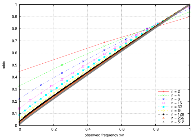
Figure 1: Odds for frequency model with linear utility function. The table shows for frequencies $x/n$ of event $E$, and the values of $q$ and $q+q^{\prime}$, as computed from (16). The value of $q^{\prime}$ can be obtained, by symmetry, from the frequency $(n-x)/n$. Values for larger $n$ are plotted in fig. 1. Only marked points are realizable values of the frequency.

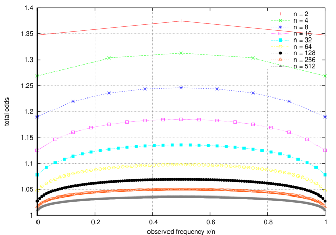
Figure 2: The total odds $s=q+q^{\prime}$ for frequency model with linear utility function. Only marked points are realizable values of the frequency.

Figure 1 shows computed odds for various observed frequencies for a small number of observations in a table, and for progressively larger numbers of observations in the graph. Figure 2 shows the total odds $s=q+q^{\prime}$. A number of interesting, but not unexpected, facts can be seen. For a small number of observations the odds are far from probabilistic, but they become more probabilistic as the number of observations increase. Furthermore, the odds deviate most from a probability for the event with a low frequency count, which is consistent with the base-rate effect. Observe that meaningful odds are given when $x=0$ or $n$, and that $q\to{}x/n$ and $q^{\prime}\to{}(n-x)/n$ as $n\to\infty$. Furthermore, we find that for a fixed ratio $x/n$, $q+q^{\prime}\to{}1+\frac{c}{\sqrt{n}}$ for some constant $c$ as $n\to\infty$.

3.2 Frequency model with logarithmic utility

This situation allows an essentially closed form solution for the odds. Using equation (12) with $\Pr(x,n\mid{}\pi)=C^{n}_{x}\pi^{x}(1-\pi)^{n-x}$ and $\Pr(\pi)=1$, obtains

$$q = \left(\frac{x+1}{n-x+1}\right)^{\frac{n-x+1}{n+2}}e^{\psi},\qquad q^{\prime}=\left(\frac{n-x+1}{x+1}\right)^{\frac{x+1}{n+2}}e^{\psi},$$

$$\psi = \left(\frac{x+1}{n+2}\right)H_{x+1}+\left(\frac{n-x+1}{n+2}\right)H_{n-x+1}-H_{n+2}$$

where we use the harmonic numbers $H_{k}=\sum_{i=1}^{k}\frac{1}{i}$.

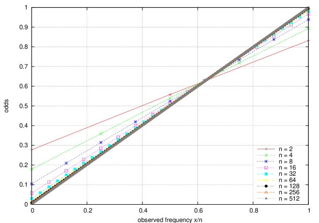
Figure 3: Odds for frequency model with logarithmic utility function. The table shows for frequencies $x/n$ of event $E$, and the values of $q$ and $q+q^{\prime}$, as computed from the closed form formula. The value of $q^{\prime}$ can be obtained, by symmetry, from the frequency $(n-x)/n$. Values for larger $n$ are plotted in fig. 1. Only marked points are realizable values of the frequency.

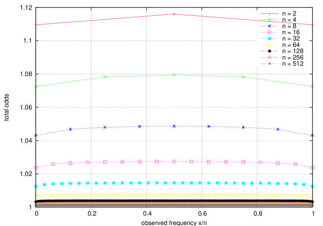
Figure 4: The total odds $s=q+q^{\prime}$ for frequency model with logarithmic utility function. Only marked points are realizable values of the frequency.

Figure 3 provides a table of computed values of the odds for small values of $n$ and graphs the odds for larger values. These computed odds should be compared with fig. 1. Figure 4 shows how the total odds $q+q^{\prime}$ varies with number of observations, which should be compared with fig. 2. It is observed that the total odds have a smaller excess over unity, and vary less with the observed fraction. This is not surprising, because a client who aims to maximise their rate of growth of wealth is less likely to exploit forecast errors of low probability events. Observe also that the odds converge much faster in this situation, at a rate of $1/n$, as opposed to $1/\sqrt{n}$ in the infinitesimal bets case. (The author also has closed form expressions for the odds in this case of an arbitrary number of events, which will discussed elsewhere.)

3.3 Gaussian model with linear utility

Now consider a situation where the forecaster is given scalar observations $D=\{x_{1},\dots,x_{n}\}$, with statistics

$$\hat{\mu} = \frac{1}{n}\sum_{i}x_{i}$$

$$\hat{\sigma}^{2} = \frac{1}{n}\sum_{i}(x_{i}-\hat{\mu})^{2}=\frac{1}{n}\sum_{i}x_{i}^{2}-\hat{\mu}^{2}.$$

Furthermore, the forecaster has reason to model these as observations of a random variable $X$ with a Gaussian distribution $N(\mu,\sigma^{2})$, for some unknown $\mu$ and $\sigma$; although the forecaster may have additional prior belief $\Pr(\mu,\sigma)$ in the values of $\mu$ and $\sigma$. The client requires an odds forecast for the events $E=\{X\leq{}x\}$ and $E^{\prime}=\{X>x\}$ for some fixed $x$.

Since we are assuming a perfect model class (to avoid third order uncertainty issues), then the true probability $\pi$ of the event $E$ is

$$\pi=\Pr(X\leq{}x)=\int_{-\infty}^{x}\frac{1}{\sqrt{2\pi\sigma^{2}}}e^{-(t-\mu)^{2}/2\sigma^{2}}\,dt=\Phi\left(\frac{x-\mu}{\sigma}\right).$$

Whereas the optimisation problem (5) that obtains the odds is formulated in terms of integrals over the probabilities of the events, in this situation we see these probabilities are determined entirely from $x$, $\mu$ and $\sigma$. Consequently, it is more appropriate to reformulate the optimisation (5) it terms of integrals over $\mu$ and $\sigma$. This requires reformulating equations (3) and (4).

When the forecaster assigns odds $q$ and $q^{\prime}$ to $E$ and $E^{\prime}$ respectively, then in the worst case where the client knows $\mu$ and $\sigma$ (and hence $\pi$) the optimal strategy of the client is to bet on

$$E \frac{q}{q+q^{\prime}}<\Phi\left(\frac{x-\mu}{\sigma}\right),$$ if

$$E^{\prime} \frac{q^{\prime}}{q+q^{\prime}}<1-\Phi\left(\frac{x-\mu}{\sigma}\right).$$ if

and the average pay-out to client is then

$$V(q,q^{\prime}\mid{}x,\mu,\sigma)=\max\left\{\frac{1}{q}\Phi\left(\frac{x-\mu}{\sigma}\right),\frac{1}{q^{\prime}}\left(1-\Phi\left(\frac{x-\mu}{\sigma}\right)\right)\right\}-1.$$

Given their model the forecaster will assert that $\Pr(\pi\mid{}D)\propto\Pr(D\mid{}\mu,\sigma)\Pr(\mu,\sigma)$ where

$$\Pr(D\mid{}\mu,\sigma) = \prod_{i=1}^{n}\frac{1}{\sqrt{2\pi\sigma^{2}}}e^{-(x_{i}-\mu)^{2}/2\sigma^{2}}$$

$$= \left(\frac{1}{\sqrt{2\pi\sigma^{2}}}\right)^{n}e^{-n(\hat{\sigma}^{2}+(\hat{\mu}-\mu)^{2})/2\sigma^{2}}.$$

Just as in section 3.1 we once again have a situation involving binary events where there is advantage in defining $s=q+q^{\prime}$, $q=ps$, $q^{\prime}=(1-p)s$, so that problem (5) can be transformed to

$$\min_{0\leq{p}\leq 1}s=\frac{1}{C}\left(\frac{A(p,x)}{1-p}+\frac{B(p,x)}{p}\right),$$

where

$$A(p,x) = \int_{0}^{\infty}\int_{M(p,x,\sigma)}^{\infty}\Phi\left(\frac{x-\mu}{\sigma}\right)F(\mu,\sigma)\,d\mu\,d\sigma,$$

$$B(p,x) = \int_{0}^{\infty}\int_{-\infty}^{M(p,x,\sigma)}\left(1-\Phi\left(\frac{x-\mu}{\sigma}\right)\right)F(\mu,\sigma)\,d\mu\,d\sigma,$$

$$C = \int_{0}^{\infty}\int_{-\infty}^{\infty}F(\mu,\sigma)\,d\mu\,d\sigma,$$

$$M(p,x,\sigma) = x-\sigma\Phi^{-1}(p),$$

$$F(\mu,\sigma) = \Pr(D\mid{}\mu,\sigma)\Pr(\mu,\sigma).$$

The odds can be calculated once the prior $\Pr(\mu,\sigma)$ has been assigned, however, the assignment of the prior requires a little care. It is not unreasonable to assume no knowledge of $\mu$, and hence place a uniform prior on $\mu$. On the other hand, one cannot assume a uniform prior for $\sigma$, because the integrals will diverge. Taking a uniform prior for $\sigma$ on $(0,R)$, then one finds that $s\to 1$ and $p\to 1/2$ as $R\to\infty$. Essentially a model that freely allows arbitrarily large variances cannot provide useful forecasts. Consequently, one is required to specify a prior for $\sigma$ with a tail that thins sufficiently rapidly.

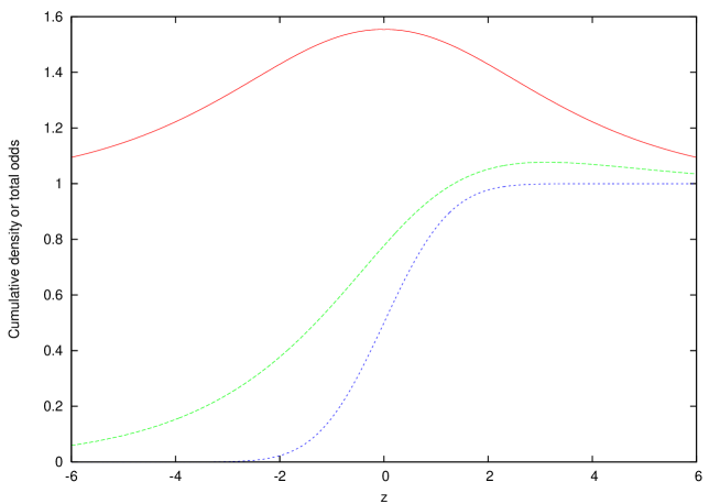
Figure 5: Odds $q$ (dashed) and total odds $s=q+q^{\prime}$ (solid) for Gaussian model with linear utility function, here computed for the generic situation $\hat{\mu}=0$ and $\hat{\sigma}=1$, prior $\Pr(\mu,\sigma)=\sigma{}e^{-\sigma^{2}}$, and events $E=\{Z\leq{}z\}$ and $E^{\prime}=\{Z>z\}$. The standard normal cumulative distribution function is also plotted for comparison (dotted).

Figure 5 shows numerically computed odds for a situation where $\hat{\mu}=0$ and $\hat{\sigma}=1$. The prior used was $\Pr(\mu,\sigma)=\sigma e^{-\sigma^{2}/2}$, which is a $\chi$-distribution of two degrees of freedom. This prior was used because we want $\hat{\sigma}=1$ to be a typical observed value. The computed odds were similar for half-normal, F-distributions and other similar distributions where $\hat{\sigma}=1$ is a typical observed value. By a shift and scale the computed odds shown in fig. 5 provide a general solution for arbitrary $\hat{\mu}$ and $\hat{\sigma}$. Let $x_{i}=\hat{\mu}+\hat{\sigma}z_{i}$ so that the $z_{i}$ have mean zero and variance one. These $z_{i}$ should be modelled as observations of a random variable $Z=(X-\hat{\mu})/\hat{\sigma}$. The events of interested are now expressed as $E=\{Z\leq{}z\}$ and $E^{\prime}=\{Z>z\}$, where $x=\hat{\mu}+\hat{\sigma}z$. Hence, if $q(z)$ and $s(z)$ represent the odds and total odds for the generic case shown in fig. 5, then the odds in the general case are obtained using $z=(x-\hat{\mu})/\hat{\sigma}$.

Figure 5 shows that the odds on $E$ exceed one for $z$ larger than about 1. Our interpretation of this is that given the information available to the forecaster, the event $E$ is so likely that offering odds favourable to the client would be loss making to the forecaster. The client is therefore offered odds so that to bet on $E$ makes a consistent small loss with an rare loss of $-1$, and to bet on $E^{\prime}$ makes a consistent loss of $-1$ and a rare win.

3.4 Gaussian model with logarithmic utility

Computation of odds in this situation follow in a similar fashion to the previous section, in that the integrals (12) are reformulated in terms of integrals over $\mu$ and $\sigma$. Thus, using the same notation as the previous sections, the odds are $q=\bar{\pi}e^{\alpha}$ and $q^{\prime}=(1-\bar{\pi})e^{\alpha}$ where

$$\bar{H} = \frac{1}{C}\int_{0}^{\infty}\int_{-\infty}^{\infty}\Phi((z-\mu)/\sigma)\log(\Phi((z-\mu)/\sigma))F(\mu,\sigma)\,d\mu\,d\sigma,$$

$$+\frac{1}{C}\int_{0}^{\infty}\int_{-\infty}^{\infty}(1-\Phi((z-\mu)/\sigma))\log(1-\Phi((z-\mu)/\sigma))F(\mu,\sigma)\,d\mu\,d\sigma,$$

$$\bar{\pi} = \frac{1}{C}\int_{0}^{\infty}\int_{-\infty}^{\infty}\Phi((z-\mu)/\sigma)F(\mu,\sigma)\,d\mu\,d\sigma,$$

$${\alpha} = \bar{H}-\bar{\pi}\log(\bar{\pi})-(1-\bar{\pi})\log(1-\bar{\pi})$$

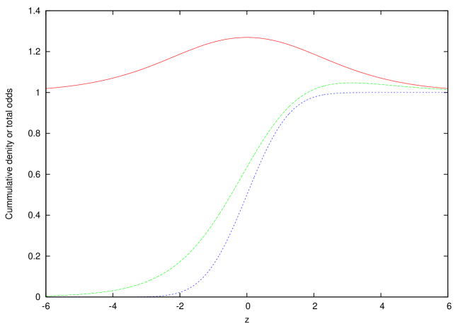
Figure 6: Odds $q$ (dashed) and total odds $s=e^{\alpha}$ (solid) for Gaussian model with logarithmic utility function, here computed for the generic situation $\hat{\mu}=0$ and $\hat{\sigma}=1$, prior $\Pr(\mu,\sigma)=\sigma{}e^{-\sigma^{2}}$, and events $E=\{Z\leq{}z\}$ and $E^{\prime}=\{Z>z\}$. The standard normal cumulative distribution function is also plotted for comparison (dotted).

Figure 6 shows the computed odds for a situation where $\hat{\mu}=0$ and $\hat{\sigma}=1$, and the prior $\Pr(\mu,\sigma)=\sigma e^{-\sigma^{2}/2}$. These odds should be compared with the linear utility situation shown in fig. 5. In comparison it is seen that the logarithmic utility function gives odds with smaller excess $s$ and less weight attached to the large $z$ values. this is similar to the frequency model, for the same reasons.

4 Investment and loss mitigation

The client who has featured thus far in our analysis is more accurately described as a speculative client, whose primary goal is to profit from inadequacies of the forecaster’s predictions. We now introduce the invested client, whose wealth is invested in some venture whose profit, costs, and losses are determined in part by the outcomes of the events. Think here of the road-gritter, or horticulturist who is concerned with the possibility of freezing temperatures. The invested client has no desire or ability to challenge the forecaster’s skill, rather they wish to use the forecasts to mitigate their losses. The invested client can do this by betting against the forecaster; a bet is essentially an insurance policy. In this section we analyse how an invested client should bet and show that such bets are beneficial to the invested client despite the forecaster’s odds being non-probabilistic. Furthermore, we will see that the client deals only with the forecaster’s odds, they do not try to normalise the odds to obtain probability “estimates”; the odds contain all the information the invested client needs.

4.1 Simple investment

Consider a situation where the return on a client’s investment is influenced by whether an event $E$, or its complement $E^{\prime}$, occurs. Let $R$ be the return on the investment when the event $E$ occurs and $R^{\prime}$ the return on $E^{\prime}$. Let $\pi$ and $\pi^{\prime}$, where $\pi+\pi^{\prime}=1$, be the probabilities of the events $E$ and $E^{\prime}$ respectively, under assumption that Nature selects the events at random. The expected return on the investment is $R\pi+R^{\prime}\pi^{\prime}$.

Now suppose the forecaster provides odds $q$ and $q^{\prime}$ for the events $E$ and $E^{\prime}$. The game matrix for betting of these events is (1), in terms of the pay-outs $P=(1/q)-1$ and $P^{\prime}=(1/q^{\prime})-1$. If the client places bets with the forecaster of $\lambda\geq 0$ on the event $E$ and $\lambda^{\prime}\geq 0$ on the complement event $E^{\prime}$, then the expected return to the client is

$$(R+\lambda{}P-\lambda^{\prime})\pi+(R^{\prime}-\lambda+\lambda^{\prime}P^{\prime})\pi^{\prime}.$$

If the client chooses the bets $\lambda$ and $\lambda^{\prime}$ so that $R+\lambda{}P-\lambda^{\prime}=R^{\prime}-\lambda+\lambda^{\prime}P^{\prime}$, then the client’s return is fixed and independent of $\pi$ and $\pi^{\prime}$, indeed independent of which event occurs. Under this condition

$$R-R^{\prime}=(P^{\prime}+1)\lambda^{\prime}-(P+1)\lambda=\frac{\lambda^{\prime}}{q^{\prime}}-\frac{\lambda}{q},$$

and so, if $R>R^{\prime}$, then the client should bet $\lambda=0$ and $\lambda^{\prime}=q^{\prime}(R-R^{\prime})$ for a return of $(1-q^{\prime})R+q^{\prime}R^{\prime}$, and if $R<R^{\prime}$, then the client should bet $\lambda=q(R^{\prime}-R)$ and $\lambda^{\prime}=0$ for a return of $qR+(1-q)R^{\prime}$.

Since $q+q^{\prime}>1$ the returns with bets are less than the expected return without bets, the advantage to the client is that by placing bets the return is guaranteed and the risk is transferred to the forecaster. In a market of forecasters those that offer the odds closer to being probabilities will attract more clients, but if their odds have not been calculated along the lines we have described, then they will be almost surely bankrupted.

4.2 Mitigating losses

Consider a situation where a client incurs a loss $L$ if an event $E$ occurs, but they can take an action at cost $C$ which if taken results in inclusive mitigated losses $M$. This situation is represented by the following game matrix.

client

nature

$$E$$

no action

action

In this situation it is usual that $0<C<M<L$, although it can happen that mitigating the losses includes a reward that more than covers costs of the action so that $M<C$. In either case the optimal strategy for the client is to take the action when $\pi>C/(L+C-M)$.

As before a forecaster provides odds on the events $E$ and $E^{\prime}$. Suppose the client places bets $\lambda$ and $\lambda^{\prime}$ on $E$ and $E^{\prime}$ respectively when no action is taken, and places bets $\mu$ and $\mu^{\prime}$ when the action is taken. The game matrix is the following.

$$E$$

no action

action

Following the analysis of the previous subsection there are three possibilities:

1. Take no action and place bets $\lambda=qL$ and $\lambda^{\prime}=0$, which results in a fixed loss $-qL$.

2. Given $C<M$, take the action and place bets $\mu=q(M-C)$ and $\mu^{\prime}=0$, which results in a fixed loss $-qM-(1-q)C$.

3. Given $M<C$, take the action and place bets $\mu=0$ and $\mu^{\prime}=q^{\prime}(C-M)$, which results in a fixed loss $-(1-q^{\prime})M-q^{\prime}C$.

It follows that when $0<C<M<L$ the client always bets on the event occurring and takes the action when $q>C/(L+C-M)$. In the situation where $0<M<C<L$ the client bets on the event occurring when taking no action, and bets on the event not occurring when taking the action, and takes the action when $qL-(C-M)q^{\prime}>M$. Once again if $q+q^{\prime}>1$, then the losses with bets are more than the expected losses without bets, but the losses are fixed and the forecaster takes the risk.

The important point to note about these results, and those of the previous subsection, is the client uses the odds $q$ and $q^{\prime}$ directly, and does not normalise these to obtain probability “estimates” $q/(q+q^{\prime})$ and $q^{\prime}/(q+q^{\prime})$ of the events. All the useful information to the client in contained in the odds, and whether the clients refers to both $q$ and $q^{\prime}$, or just one of these values, depends on their circumstances. For example, in the $0<C<M<L$ situation the decision to take the action is based on $q$ alone, where as, in the $0<M<C<L$ situation it depends on both $q$ and $q^{\prime}$, but not in a way that implies normalising them to obtain probability “estimates”.

5 Ensemble Forecasting

Finally we consider an example of issuing of odds forecasts on temperature variations using numerical ensemble weather predictions. A common event of interest is whether the temperature at a locality will fall below freezing. These events are fairly rare, so we consider a related and more general event of whether the temperature at a location at some set lead-time falls more than a certain amount below the current temperature at that station. These calculations are intended to provide an illustration of odds forecasting using the results we have obtained so far. We do not claim that the odds forecast we compute are the best or most appropriate, indeed the results suggest otherwise. Odds based on kernel density estimates, kernel dressing and the like could provide better odds forecasts.

5.1 Data preparation

We use London Heathrow (Station 03772) as the locality and National Center for Environmental Prediction GFS ensemble predictions (Troth, 2008) for constructing odds forecasts. The GFS model provides a temperature at the station by interpolation of the temperatures of the global circulation model’s nearest grid-points to the location. Our first step is to prepare suitable time series data including bias correction and temporal interpolation.

The GFS 2-metre-temperature deterministic-forecast initialisation states were used to calibrate GFS model temperatures with the station readings as follows. Firstly, we compute a cubic spline of the time series of deterministic-forecast initialisation states. Secondly, we compute using the spline a model temperature time-series to pair with the station temperature time-series. Finally, we fit by least squares the model

$$y=p_{0}(x)+p_{1}(x)\cos(2\pi{h}/24)+p_{2}(x)\sin(2\pi{h}/24),$$ (17)

where $y$ is the station temperature, $x$ the splined model temperature, $h$ the hour of the day, and each $p_{j}(x)$ is a cubic polynomial. This is a twelve parameter model. We used times series from the calendar year 2005. The residuals of this model had mean $6.03\times 10^{-15}$, skewness $0.0736$, kurtosis $0.9453$ and standard error of $1.1159$ degrees centigrade. Hence, this model provides a good transformation from model state temperature to station temperature with an expected error that is very nearly Gaussian and standard deviation of around $1.1159$ degrees centigrade.

To obtain ensemble forecasts at any lead-time we compute a cubic spline to the time series of each ensemble member, then apply our fitted transform (17).

In the following these interpolated and transformed time-series will be referred to as the adjusted control and the adjusted ensemble forecasts. Figure 7 shows an example of the station data, adjusted control and adjusted ensemble time-series.

5.2 Odds forecasts

The goal is to provide odds forecasts on whether the minimum daily temperature at one to ten days lead-time will be less than 3 degrees centigrade below the adjusted control temperature at the time of issuing the forecasts. In order to use the results we have already derived we consider four forecasts. The first forecast applies the odds from a frequency model, which is based on counting number of adjusted ensemble members below the target threshold. The second forecast applies the odds from a Gaussian model, which assumes the adjusted ensemble members have a Gaussian distribution. The third forecast is a probabilistic forecast obtained by assuming the adjusted ensemble members have a Gaussian distribution. The forth forecast is intended to act as the ultimate-challenge client. It is not really a forecast at all, but rather the predicted probability of station temperature being below the threshold based on a Gaussian distribution centred on the adjusted control with standard deviation equal to $1.1159$, that is, error of the fitted residuals.

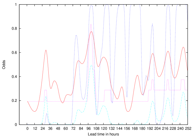
Figure 8: Four computed odds forecasts (linear utility) for the data shown in figure 7. Frequency odds (dashed), Gaussian odds (solid), and probabilistic odds (dash-dotted). Challenger (dashed) refers to the odds used by the ultimate-challenge client against whom the forecasters must compete.

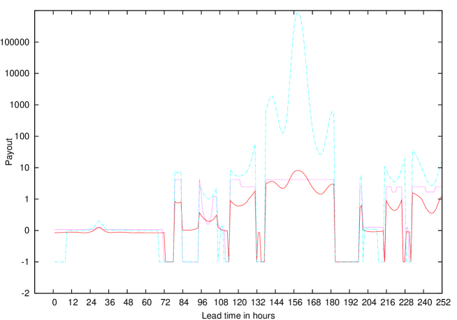
Figure 9: The pay-outs of the three forecasters when faced with the ultimate-challenge client, for linear utility. Frequency odds (dashed), Gaussian odds (solid), and probabilistic odds (dash-dotted). Same data as shown is figures 7 and 8. The pay-outs are shown on a linear scale for pay-outs less than one, then transitions into a logarithm base 10 scale above.

Forecasts one to three represent three competing forecasters, one and two providing non-probabilistic odds, three providing probabilistic odds. Forecast four is used by the ultimate-challenge client. Nature is always taken to be the station temperature. Using the methods described in the previous sections odds forecasts can be computed. Figure 8 shows the odds computed using the time-series data shown in fig. 7 in the case of a linear utility. Figure 9 shows the pay-out of the three forecasters when playing against the ultimate-challenge client. Since the challenger is using a linear utility they will bet on the temperature being below the threshold if the forecaster’s odds are less than the challenger’s odds and visa versa. Observe that the challenger loses more bets to forecaster 3, who uses probabilistic odds, than to forecasters 1 and 2, who use non-probabilistic odds, however, the winning bets on low probability events against forecaster 3 are astronomical. On the other hand, forecasters 1 and 2 appear to perform about the same.

We now consider the problem of forecasting whether the minimum temperature at London Heathrow in the 24 hour period from 18:00UTC is more than 3 degrees centigrade below the control temperature when the forecasts are issued. We will test the performance of the odds forecasts by computing the total pay-out to the ultimate-challenge client for the first half of 2005 (183 days) for lead times up to ten days. Figures 7 and 8 clearly demonstrate that the probabilistic odds we have considered are not competitive with the non-probabilistic odds. Certainly, large pay-outs result from assigning far too small probability to low probability events, but what about the performance at other times? To investigate this question we consider a new non-probabilistic odds forecaster ($3^{\prime}$) that uses the probabilistic odds but sets minimum odds of $0.1$, which effectively caps pay-outs at 10. These capped probabilities are a crude form of odds. Odds capping could be applied by our forecasters 1 and 2, although in the test considered it makes little difference. Table 1 shows the total pay-out to the three non-probabilistic odds forecasters 1, 2, and $3^{\prime}$, on bets taken from the ultimate-challenge client. If forecasters 1 and 2 are allowed odds caps of $0.1$ is these tests, then the cap only applies on around ten occasions and reduces the larger pay-outs at lead times 5, 7, and 10 days to the level of their neighbouring lead times.

A number of observations can be made about the results displayed in table 1. Recall that the aim of the forecasters is to have an expected total pay-out of zero. It is immediately clear that odds capping alone is not sufficient to make forecaster $3^{\prime}$ competitive with forecasters 1 and 2 beyond a lead time of one or two days. Forecasters 1 and 2 have similar performance although forecaster 2 is more successful. In all cases it appears that performance decreases with increasing lead time.

6 Summary, discussion and conclusions

We have confronted forecasters with the challenge that if they offer a probability forecast, then they should be prepared to accept bets at the odds these imply. Unless a forecaster has a perfect forecast model, then they would be unwise to accept this challenge, because any that do so will almost surely be bankrupted by more informed bettors. We argue that probability forecasts fail to account for higher order uncertainties, such as model error. Our alternative is to offer non-probabilistic odds forecasts obtain using an optimisation principle. The excess of the odds reveals the forecaster’s uncertainty about the model. We have shown how to compute odds forecasts in several situations, and illustrated how odds forecasts could be used in investment, loss mitigation, and weather forecasting.

There are gaps in our development and demonstrations, especially in the application to ensemble weather forecasting. A gap occurs because we have only shown how to compute odds under the assumption of a perfect model class; this assumption eliminates third and higher order uncertainties. Figure 7 shows that an assumption of a perfect model class is not well supported in our application to ensemble weather forecasting, because during lead-times of 144 to 180 hours the entire forecast ensemble fails to represent what actually happened. This implies the assumption that the ensemble is random selection form the distribution of possibilities is false. Nonetheless, table 1 shows that our odds calculation is sufficiently conservative at these lead times to cope fairly well with this level of uncertainty; pay-outs of around 50 units compared to 200 units for capped probabilities. The goal, however, was that the pay-outs should be zero on average. It would be optimistic to suggest this were the case for lead times of 5 days or more. Improvement of these odds forecasts is certainly possible. Either by more careful consideration of the selection of the prior, or by abandoning the simple frequency and Gaussian models for a more sophisticated model that takes into account the conditional aspects of the weather. In analogy to the urn game, a more sophisticated model means looking more closely at the mixing process.

We have argued that odds forecasting has uses in investment and loss mitigation, we claim also that it can be used for model assessment. The results of table 1 suggest that the Gaussian model is quite successful out to lead times of 5 days. Kernel-density based models may well do better, extending to longer lead times, or having average pay-outs closer to zero. Comparison with an ultimate-challenge client as we do provides a diagnostic of the models performance, and furthermore, if a model achieves a zero average pay-out, then excess of the odds provide indications of the model’s higher order uncertainty.

$x/n$ $q$ $q+q^{\prime}$ $0/1$ 0.556 1.411 $1/1$ 0.855 1.411 $0/2$ 0.448 1.347 $1/2$ 0.687 1.375 $2/2$ 0.900 1.347 $0/3$ 0.378 1.302 $1/3$ 0.578 1.336 $2/3$ 0.758 1.336 $3/3$ 0.924 1.302 $0/4$ 0.329 1.268 $1/4$ 0.501 1.303 $2/4$ 0.656 1.313 $3/4$ 0.803 1.303 $4/4$ 0.939 1.268

$x/n$ $q$ $q+q^{\prime}$ $0/1$ 0.382 1.146 $1/1$ 0.764 1.146 $0/2$ 0.277 1.11 $1/2$ 0.558 1.116 $2/2$ 0.832 1.11 $0/3$ 0.217 1.087 $1/3$ 0.438 1.094 $2/3$ 0.656 1.094 $3/3$ 0.87 1.087 $0/4$ 0.179 1.073 $1/4$ 0.359 1.078 $2/4$ 0.54 1.079 $3/4$ 0.719 1.078 $4/4$ 0.894 1.073

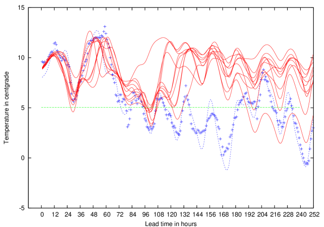
Figure 7: Station temperature time series $(+)$, the adjusted control (dashed) and adjusted ensemble forecast time-series (solid). The horizontal line (dashed) shows the threshold line for which the odds forecasts are required. The forecasts shown were launched 00:00UTC day 40 of 2005.

Utility	Linear			Logarithmic
Lead	1.	2.	$3^{\prime}$.	1.	2.	$3^{\prime}$.
time	Freq.	Gaus.	Capped	Freq.	Gaus.	Capped
(days)	odds	odds	Prob.	odds	odds	Prob.
1	7.3	47.6	36.2	-1.19	-4.03	4.94
2	65.5	-11.7	160	8.97	-2	12.5
3	117	14.9	233	20.3	5.21	21.6
4	78.9	3.75	175	16.6	5.28	20.8
5	70.9	68.2	186	14.1	4.54	18.8
6	73.7	7.71	166	15.6	6.29	20
7	80.5	82.6	196	20.5	13.1	26.2
8	105	24.3	238	21	9.89	27.6
9	124	50.1	283	28.5	18	34.4
10	147	130	325	33.5	22.9	38.1

Table 1: Total pay-out of forecasters on bets taken from the ultimate-challenge client on the event that the minimum temperature at London Heathrow in the 24 hours period from 18:00UTC is more than 3 degrees centigrade below the control temperature when the forecasts are issued. Total computed over first half of 2005. In the case of logarithmic utility the pay-out is expressed as the logarithm base 10.

References

- Brier [1950] G.W. Brier. Verification of forecasts expressed in terms of probability. Monthly Weather Review, 78(1):1–3, 1950.
- Dawid [2004] A.P. Dawid. Probability, causality, and the empirical world : A Bayes–de Vinetti–Popper–Borel synthesis. Statistical Science, 19(1):44–57, 2004.
- Doob [1953] J.L. Doob. Stochastic processes. Wiley and Sons, 1953.
- Foster and Vohra [1998] D.P. Foster and R.V. Vohra. Asymptotic calibration. Biometrika, 85(2):379–390, 1998.
- Foster and Vovk [1999] D.P. Foster and R. Vovk. Regret in the on-line decision problem. Games and Economic Behavior, 29:7–35, 1999.
- Granger and Pesaran [2000] C.W.J. Granger and M.H. Pesaran. Economic and statistical measures of forecast accuracy. Journal of Forecasting, 19(7):537–560, 2000.
- Johnstone [2007] D. Johnstone. Economic Darwinism : who has the best probabilities? Theory and Decision, 62:47–96, 2007.
- Kelly [1956] J. Kelly. A new interpretation of information rate. Bell Systems Technical Journal, 35:916–926, 1956.
- Levitt [2004] S.D. Levitt. Why gambling markets organized so differently from financial markets? The Economic Journal, 114:223–246, 2004.
- Murphy [1993] A.H. Murphy. What is a good forecast? an essay on the nature of goodness in weather forecasting. Weather and Forecasting, 8(2):281–293, 1993.
- Murphy and Winkler [1977] A.H. Murphy and R.L. Winkler. Reliability of subjective probability forecasts of precipitation and temperature. Applied Statistics, 26:41–47, 1977.
- Murphy and Winkler [1987] A.H. Murphy and R.L. Winkler. A general framework for forecast verification. Monthly Weather Review, 115:1330–1338, 1987.
- Oakes [1985] D. Oakes. Self-calibrating priors do not exist. J. Am. Statist. Assoc., 80:339–, 1985.
- Palmer [2000] T. Palmer. Predicting uncertainty in forecasts of weather and climate. Rep. Prog. Physics, 63:71–116, 2000.
- Press et al. [1988] W. H. Press, B. P. Flannery, S. A. Teukolsky, and W. T. Vetterling. Numerical Recipes in C. Cambridge University Press, Cambridge, 1988.
- Roulston and Smith [2002] M.S. Roulston and L.A. Smith. Evaluating probabilistic forecasts using information theory. Monthly Weather Review, 130(6):1653–1660, 2002.
- Shafer and Vovk [2001] G. Shafer and V.G. Vovk. Probability and Finance : It’s all a game. Wiley, 2001.
- Skouras and Dawid [1999] K. Skouras and A.P. Dawid. On efficient probability forecasting systems. Biometrika, 86, 1999.
- Smith [1995] L.A. Smith. Accountability and error in ensemble forecasting. In Predictability, volume 1 of ECMWF Seminar Proceedings, pages 351–369, Shinfield Park, Reading, Berkshire, RG29ax, september 95 1995. ECMWF.
- Troth [2008] Z. Troth. NCEP ensemble products. http://wwwt.emc.ncep.noaa.gov/gmb/ens, 2008.
- von Neumann and Morgenstern [1944] J. von Neumann and O. Morgenstern. Theory of Games and Economic Behavior. reprinted Dover, 1944.
- Williams [1991] D. Williams. Probability With Martingales. Cambridge Univ. Press, 1991.
- Winkler [1994] R.L. Winkler. Evaluating probabilities: Asymmetric scoring rules. Management Science, 40(11):1395–1405, 1994.