Strong $\Sigma_{b}NB$ and $\Sigma_{c}ND$ coupling constants in QCD

We study the strong interactions among the heavy bottom spin–1/2 $\Sigma_{b}$ baryon, nucleon and $B$ meson as well as the heavy charmed spin–1/2 $\Sigma_{c}$ baryon, nucleon and $D$ meson in the context of QCD sum rules. We calculate the corresponding strong coupling form factors defining these vertices by using a three point correlation function. We obtain the numerical values of the corresponding strong coupling constants via the most prominent structure entering the calculations.

PACS number(s): 13.30.-a, 13.30.Eg, 11.55.Hx

1 Introduction

In the recent years, substantial experimental improvements have been made on the spectroscopic and decay properties of heavy hadrons, which were accompanied by theoretical studies on various properties of these hadrons. The mass spectrum of the baryons containing heavy quark has been studied using different methods. The necessity of a deeper understanding of heavy flavor physics requires a comprehensive study on the processes of these baryons such as their radiative, strong and weak decays. For some of related studies one can refer to references [1, 2, 3, 4, 5, 6, 7, 8, 9, 10].

The investigation of the strong decays of heavy baryons can help us get valuable information on the perturbative and non-perturbative natures of QCD. The strong coupling constants defining such decays play important role in describing the strong interaction among the heavy baryons and other participated particles. Therefore, accurate determination of these coupling constants enhance our understanding on the interactions as well as the nature and structure of the participated particles. The present work is an extension of our previous study on the coupling constants $g_{\Lambda_{b}NB}$ and $g_{\Lambda_{c}ND}$ [11]. Here, we study the strong interactions among the heavy bottom spin–1/2 $\Sigma_{b}$ baryon, nucleon and $B$ meson as well as the heavy charmed spin–1/2 $\Sigma_{c}$ baryon, nucleon and $D$ meson in the context of QCD sum rules. In particular, we calculate the strong coupling constants $g_{\Sigma_{b}NB}$ and $g_{\Sigma_{c}ND}$. These coupling constants together with the $g_{\Lambda_{b}NB}$ and $g_{\Lambda_{c}ND}$ discussed in our previous work, may also be used in the bottom and charmed mesons clouds description of the nucleon which can be used to explain the exotic events observed by different Collaborations. In addition, the determination of the properties of the $B$ and $D$ mesons in nuclear medium requires the consideration of their interactions with the nucleons from which the $\Lambda_{b[c]}$ and $\Sigma_{b[c]}$ are produced. Therefore, to determine the modifications on the masses, decay constants and other parameters of the $B$ and $D$ mesons in nuclear medium, one needs to consider the contributions of the baryons $\Sigma_{b[c]}$ together with the $\Lambda_{b[c]}$ and have the values of the strong coupling constants $g_{\Sigma_{b}NB}$ and $g_{\Sigma_{c}ND}$ besides the couplings $g_{\Lambda_{b}NB}$ and $g_{\Lambda_{c}ND}$  [12, 13, 14, 15]. In the literature, one can unfortunately find only a few works on the strong couplings of the heavy baryons with the nucleon and heavy mesons. One approximate prediction for the strong coupling $g_{\Lambda_{c}ND}$ was made at zero transferred momentum squared [4]. The strong couplings of the charmed baryons with the nucleon and $D$ meson were also discussed in [7] in the framework of light cone QCD sum rules.

This paper is organized in three sections as follows. In the next section, we present the details of the calculations of the strong coupling form factors among the particles under consideration. In section 3, the numerical analysis of the obtained sum rules and discussions about the results are presented.

2 Theoretical framework

This section is devoted to the details of the calculations of the strong coupling form factors $g_{\Sigma_{b}NB}(q^{2})$ and $g_{\Sigma_{c}ND}(q^{2})$ from which the strong coupling constants among the participating particles are obtained at $Q^{2}=-q^{2}=-m_{B[D]}^{2}$, subsequently. In order to accomplish this purpose, the following three-point correlation function is used:

$$\Pi=i^{2}\int d^{4}x~{}\int d^{4}y~{}e^{-ip\cdot x}~{}e^{ip^{\prime}\cdot y}~{}{\langle}0|{\cal T}\left(\eta_{N}(y)~{}\eta_{B[D]}(0)~{}\bar{\eta}_{\Sigma_{b}[\Sigma_{c}]}(x)\right)|0{\rangle},$$ (1)

whith ${\cal T}$ being the time ordering operator and $q=p-p^{\prime}$ is the transferred momentum. The currents $\eta_{N}$, $\eta_{B[D]}$ and $\eta_{\Sigma_{b}[\Sigma_{c}]}$ presented in Eq. (1) correspond to the the interpolating currents of the $N$, $B[D]$ and $\Sigma_{b[c]}$, respectively and their explicit expressions can be given in terms of the quark field operators as

$$\eta_{\Sigma_{b}[\Sigma_{c}]}(x) = \varepsilon_{ijk}\Big{(}u^{i^{T}}(x)C\gamma_{\mu}d^{j}(x)\Big{)}\gamma_{5}\gamma_{\mu}b[c]^{k}(x),$$

$$\eta_{N}(y) = \varepsilon_{ijk}\Big{(}u^{i^{T}}(y)C\gamma_{\mu}u^{j}(y)\Big{)}\gamma_{5}\gamma_{\mu}d^{k}(y),$$

$$\eta_{B[D]}(0) = \bar{u}(0)\gamma_{5}b[c](0),$$ (2)

where $C$ denotes the charge conjugation operator; and $i$, $j$ and $k$ are color indices.

In the course of calculation of the three-point correlation function one follows two different ways. The first way is called as OPE side and the calculation is made in deep Euclidean region in terms of quark and gluon degrees of freedom using the operator product expansion. The second way is called as hadronic side and the hadronic degrees of freedoms are considered to perform this side of the calculation. The QCD sum rules for the coupling form factors are attained via the match of these two sides. The contributions of the higher states and continuum are suppressed by a double Borel transformation applied to both sides with respect to the variables $p^{2}$ and $p^{\prime 2}$.

2.1 OPE Side

For the calculation of the OPE side of the correlation function which is done in deep Euclidean region, where $p^{2}\rightarrow-\infty$ and $p^{\prime 2}\rightarrow-\infty$, one puts the interpolating currents given in Eq. (2) into the correlation function, Eq. (1). Possible contractions of all quark pairs via Wick’s theorem leads to

$$\Pi^{OPE} = i^{2}\int d^{4}x\int d^{4}ye^{-ip\cdot x}e^{ip^{\prime}\cdot y}\varepsilon_{abc}\varepsilon_{ij\ell}$$ (3)

$$\times \Bigg{\{}\gamma_{5}\gamma_{\nu}S^{cj}_{d}(y-x)\gamma_{\mu}CS_{u}^{bi^{T}}(y-x)C\gamma_{\nu}S^{ah}_{u}(y)\gamma_{5}S_{b[c]}^{h\ell}(-x)\gamma_{\mu}\gamma_{5}$$

$$- \gamma_{5}\gamma_{\nu}S^{cj}_{d}(y-x)\gamma_{\mu}CS_{u}^{ai^{T}}(y-x)C\gamma_{\nu}S^{bh}_{u}(y)\gamma_{5}S_{b[c]}^{h\ell}(-x)\gamma_{\mu}\gamma_{5}\Bigg{\}}~{},$$

where $S_{b[c]}(x)$ and $S_{u[d]}(x)$ are the heavy and light quark propagators whose explicit forms can be found in Refs. [16, 11].

After some straightforward calculations (for details refer to the Ref. [11]), the correlation function in OPE side comes out in terms of different Dirac structures as

$$\Pi^{OPE} = \Pi_{1}(q^{2})\gamma_{5}+\Pi_{2}(q^{2})\!\not\!{p}\gamma_{5}+\Pi_{3}(q^{2})\!\not\!{q}\!\not\!{p}\gamma_{5}+\Pi_{4}(q^{2})\!\not\!{q}\gamma_{5}.$$ (4)

Each $\Pi_{i}(q^{2})$ function involves the perturbative and non-perturbative parts and is written as

$$\Pi_{i}(q^{2})=\int ds\int ds^{\prime}\frac{\rho_{i}^{pert}(s,s^{\prime},q^{2})+\rho_{i}^{non-pert}(s,s^{\prime},q^{2})}{(s-p^{2})(s^{\prime}-p^{\prime^{2}})}~{}.$$ (5)

The spectral densities, $\rho_{i}(s,s^{\prime},q^{2})$, appearing in Eq. (5) are obtained from the imaginary parts of the $\Pi_{i}$ functions, i.e., $\rho_{i}(s,s^{\prime},q^{2})=\frac{1}{\pi}Im[\Pi_{i}]$. Here to provide examples of the explicit forms of the spectral densities, among the Dirac structures presented above, we only present the results obtained for the Dirac structure $\!\not\!{p}\gamma_{5}$, that is $\rho_{2}^{pert}(s,s^{\prime},q^{2})$ and $\rho_{2}^{non-pert}(s,s^{\prime},q^{2})$, which are obtained as

$$\rho_{2}^{pert}(s,s^{\prime},q^{2}) = \int_{0}^{1}dx\int_{0}^{1-x}dy\frac{1}{32\pi^{4}(x+y-1)^{2}}\Bigg{\{}2m_{b[c]}^{3}x\Big{(}3x^{2}-y-2x+3xy\Big{)}$$ (6)

$$- 3m_{b[c]}^{2}x(x+y-1)\Big{[}-m_{u}(x+4y-2)+m_{d}(3x+6y-2)\Big{]}$$

$$- q^{2}m_{b[c]}x\Big{[}y-3y^{2}+x^{2}(8y-1)+x(1-6y+8y^{2})\Big{]}+m_{b[c]}(x+y-1)$$

$$\times \Big{[}sx(8x^{2}-3y-5x+8xy)+s^{\prime}\Big{(}8xy^{2}-5xy-2y^{2}-x^{2}+8x^{2}y\Big{)}\Big{]}$$

$$- (x+y-1)\Big{[}3m_{d}s\Big{(}4x^{3}+y-y^{2}-7x^{2}+12x^{2}y+3x-12xy+8xy^{2}\Big{)}$$

$$+ 3m_{d}q^{2}y\Big{(}4x-4x^{2}+y-8xy\Big{)}+3m_{d}s^{\prime}y\Big{(}3-7x+4x^{2}-11y+12xy+8y^{2}\Big{)}\Big{]}$$

$$- m_{u}s\Big{[}4x^{3}+y(3-2y)+x^{2}(20y-13)+x(9-27y+16y^{2})\Big{]}$$

$$+ m_{u}s^{\prime}y\Big{(}9-14x+4x^{2}-26y+20xy+16y^{2}\Big{)}$$

$$+ m_{u}q^{2}y(11x-4x^{2}+2y-16xy-3)\Bigg{\}}\Theta\Big{[}L_{2}(s,s^{\prime},q^{2})\Big{]},$$

and

$$\rho_{2}^{non-pert}(s,s^{\prime},q^{2}) = \Big{\{}\frac{\langle u\bar{u}\rangle}{24\pi^{2}(q^{2}-m_{b[c]}^{2})}\Big{(}3m_{b[c]}m_{d}-3m_{u}m_{d}+3m_{u}^{2}-q^{2}+s-s^{\prime}\Big{)}$$ (7)

$$+ \langle\alpha_{s}\frac{G^{2}}{\pi}\rangle\frac{m_{b[c]}\Big{(}3q^{2}-3m_{b[c]}^{2}-2s^{\prime}\Big{)}}{192\pi^{2}(q^{2}-m_{b[c]}^{2})^{2}}+\frac{m_{0}^{2}\langle u\bar{u}\rangle}{16\pi^{2}(q^{2}-m_{b}^{2})}\Bigg{\}}\Theta\Big{[}L_{1}(s,s^{\prime},q^{2})\Big{]}$$

$$- \Big{(}\langle d\bar{d}\rangle-\langle u\bar{u}\rangle\Big{)}\int_{0}^{1}dx\int_{0}^{1-x}dy\frac{3x+6y-2}{4\pi^{2}}\Theta\Big{[}L_{2}(s,s^{\prime},q^{2})\Big{]},$$

where $\Theta[...]$ stands for the unit-step function and $L_{1}(s,s^{\prime},q^{2})$ and $L_{2}(s,s^{\prime},q^{2})$ are defined as

$$L_{1}(s,s^{\prime},q^{2}) = s^{\prime},$$

$$L_{2}(s,s^{\prime},q^{2}) = -m_{b[c]}^{2}x+sx-sx^{2}+s^{\prime}y+q^{2}xy-sxy-s^{\prime}xy-s^{\prime}y^{2}.$$ (8)

2.2 Hadronic Side

On the hadronic side, considering the quantum numbers of the interpolating fields one place the complete sets of intermediate $\Sigma_{b}[\Sigma_{c}]$, $B[D]$ and $N$ hadronic states into the correlation function. After carrying out the four-integrals, we get

$$\Pi^{HAD} = \frac{\langle 0\mid\eta_{N}\mid N(p^{\prime})\rangle\langle 0\mid\eta_{B[D]}\mid B[D](q)\rangle\langle\Sigma_{b}[\Sigma_{c}](p)\mid\bar{\eta}_{\Sigma_{b}[\Sigma_{c}]}\mid 0\rangle}{(p^{2}-m_{\Sigma_{b}[\Sigma_{c}]}^{2})(p^{\prime^{2}}-m_{N}^{2})(q^{2}-m_{B[D]}^{2})}$$ (9)

$$\times \langle N(p^{\prime})B[D](q)\mid\Sigma_{b}[\Sigma_{c}](p)\rangle+\cdots~{}.$$

In the above equation, the contributions of the higher states and continuum are denoted by $\cdots$ and the matrix elements are represented in terms of the hadronic parameters as follows:

$$\langle 0\mid\eta_{N}\mid N(p^{\prime})\rangle = \lambda_{N}u_{N}(p^{\prime},s^{\prime}),$$

$$\langle\Sigma_{b}(p)\mid\bar{\eta}_{\Sigma_{b}[\Sigma_{c}]}\mid 0\rangle = \lambda_{\Sigma_{b}[\Sigma_{c}]}\bar{u}_{\Sigma_{b}[\Sigma_{c}]}(p,s),$$

$$\langle 0\mid\eta_{B[D]}\mid B[D](q)\rangle = i\frac{m_{B[D]}^{2}f_{B[D]}}{m_{u}+m_{b[c]}},$$

$$\langle N(p^{\prime})B[D](q)\mid\Sigma_{b}[\Sigma_{c}](p)\rangle = g_{\Sigma_{b}NB[\Sigma_{c}ND]}\bar{u}_{N}(p^{\prime},s^{\prime})i\gamma_{5}u_{\Sigma_{b}[\Sigma_{c}]}(p,s).$$ (10)

Here $\lambda_{N}$ and $\lambda_{\Sigma_{b}[\Sigma_{c}]}$ are residues of the $N$ and $\Sigma_{b}[\Sigma_{c}]$ baryons, respectively, $f_{B[D]}$ is the leptonic decay constant of $B[D]$ meson and $g_{\Sigma_{b}NB[\Sigma_{c}ND]}$ is the strong coupling form factor among $\Sigma_{b}[\Sigma_{c}]$, $N$ and $B[D]$ particles. Using Eq. (2.2) in Eq. (9) and summing over the spins of the particles, we obtain

$$\Pi^{HAD} = i^{2}\frac{m_{B[D]}^{2}f_{B[D]}}{m_{b[c]}+m_{u}}\frac{\lambda_{N}\lambda_{\Sigma_{b}[\Sigma_{c}]}g_{\Sigma_{b}NB[\Sigma_{c}ND]}}{(p^{2}-m_{\Sigma_{b}[\Sigma_{c}]}^{2})(p^{\prime^{2}}-m_{N}^{2})(q^{2}-m_{B[D]}^{2})}$$ (11)

$$\times \Big{\{}(m_{N}m_{\Sigma_{b}[\Sigma_{c}]}-m_{\Sigma_{b}[\Sigma_{c}]}^{2})\gamma_{5}+(m_{\Sigma_{b}[\Sigma_{c}]}-m_{N})\not\!p\gamma_{5}+\not\!q\not\!p\gamma_{5}-m_{\Sigma_{b}[\Sigma_{c}]}\not\!q\gamma_{5}\Big{\}}$$

$$+ \cdots~{}.$$

To acquire the final form of the hadronic side of the correlation function we perform the double Borel transformation with respect to the initial and final momenta squared,

$$\widehat{\textbf{B}}\Pi^{HAD} = i^{2}\frac{m_{B[D]}^{2}f_{B[D]}}{m_{b[c]}+m_{u}}\frac{\lambda_{N}\lambda_{\Sigma_{b}[\Sigma_{c}]}g_{\Sigma_{b}NB[\Sigma_{c}ND]}}{(q^{2}-m_{B[D]}^{2})}e^{-\frac{m_{\Sigma_{b}[\Sigma_{c}]}^{2}}{M^{2}}}e^{-\frac{m_{N}^{2}}{M^{\prime^{2}}}}$$ (12)

$$\times \Big{\{}(m_{N}m_{\Sigma_{b}[\Sigma_{c}]}-m_{\Sigma_{b}[\Sigma_{c}]}^{2})\gamma_{5}+(m_{\Sigma_{b}[\Sigma_{c}]}-m_{N})\not\!p\gamma_{5}+\not\!q\not\!p\gamma_{5}-m_{\Sigma_{b}[\Sigma_{c}]}\not\!q\gamma_{5}\Big{\}}$$

$$+ \cdots~{},$$

where $M^{2}$ and $M^{\prime^{2}}$ are Borel mass parameters.

As it was already stated, the match of the hadronic and OPE sides of the correlation function in Borel scheme provides us with the QCD sum rules for the strong form factors. The consequence of that match for $\!\not\!{p}\gamma_{5}$ structure leads us to

$$g_{\Sigma_{b}NB[\Sigma_{c}ND]}(q^{2})=-e^{\frac{m_{\Sigma_{b}[\Sigma_{c}]}^{2}}{M^{2}}}e^{\frac{m_{N}^{2}}{M^{\prime^{2}}}}~{}\frac{(m_{b[c]}+m_{u})(q^{2}-m_{B[D]}^{2})}{m_{B[D]}^{2}f_{B[D]}\lambda_{\Sigma_{b}[\Sigma_{c}]}^{{\dagger}}\lambda_{N}(m_{N}m_{\Sigma_{b}[\Sigma_{c}]}-m_{\Sigma_{b}[\Sigma_{c}]}^{2})}$$

$$\times \Bigg{\{}\int^{s_{0}}_{(m_{b[c]}+m_{u}+m_{d})^{2}}ds\int^{s^{\prime}_{0}}_{(2m_{u}+m_{d})^{2}}ds^{\prime}e^{-\frac{s}{M^{2}}}e^{-\frac{s^{\prime}}{M^{\prime^{2}}}}\Big{[}\rho_{2}^{pert}(s,s^{\prime},q^{2})+\rho_{2}^{non-pert}(s,s^{\prime},q^{2})\Big{]}\Bigg{\}}~{},$$

where $s_{0}$ and $s^{\prime}_{0}$ are continuum thresholds in $\Sigma_{b}[\Sigma_{c}]$ and $N$ channels, respectively.

3 Numerical analysis

Having obtained the QCD sum rules for the strong coupling form factors, in this section, we present the numerical analysis of our results and discuss the dependence of the strong coupling form factors under consideration on $Q^{2}=-q^{2}$. To this aim, beside the input parameters given in table 1, one needs to determine the working intervals of four auxiliary parameters $M^{2}$, $M^{\prime 2}$, $s_{0}$ and $s^{\prime}_{0}$. These parameters originate from the double Borel transformation and continuum subtraction. The determination of the working regions of them is made on the basis of that the results obtained for the strong coupling form factors be roughly independent of these helping parameters.

The continuum thresholds $s_{0}$ and $s^{\prime}_{0}$ are the parameters related to the beginning of the continuum in the initial and final channels. If the ground state masses are given by $m$ and $m^{\prime}$ for the initial and final channels, respectively, to excite the particle to the first excited state having the same quantum numbers with them one needs to provide the energies $\sqrt{s_{0}}-m$ and $\sqrt{s^{\prime}_{0}}-m^{\prime}$. For the considered transitions, these quantities can be determined from well known excited states of the initial and final states [17] which are roughly in between $0.1~{}\mbox{GeV}$ and $0.3~{}\mbox{GeV}$. From these intervals, the working regions for the continuum thresholds are determined as $34.9[6.5]~{}\mbox{GeV${}^{2}$}\leq s_{0}\leq 37.4[7.6]~{}\mbox{GeV${}^{2}$}$ and $1.04~{}\mbox{GeV${}^{2}$}\leq s^{\prime}_{0}\leq 1.99~{}\mbox{GeV${}^{2}$}$ for the vertex $\Sigma_{b}NB[\Sigma_{c}ND]$.

Parameters	Values
$m_{b}$	$(4.18\pm 0.03)~{}\mbox{GeV}$[17]
$m_{c}$	$(1.275\pm 0.025)~{}\mbox{GeV}$[17]
$m_{d}$	$4.8^{+0.5}_{-0.3}~{}\mbox{MeV}$[17]
$m_{u}$	$2.3^{+0.7}_{-0.5}~{}\mbox{MeV}$ [17]
$m_{B}$	$(5279.26\pm 0.17)~{}\mbox{MeV}$ [17]
$m_{D}$	$(1864.84\pm 0.07)~{}\mbox{MeV}$ [17]
$m_{N}$	$(938.272046\pm 0.000021)~{}\mbox{MeV}$ [17]
$m_{\Sigma_{b}}$	$(5811.3\pm 1.9)~{}\mbox{MeV}$ [17]
$m_{\Sigma_{c}}$	$(2452.9\pm 0.4)~{}\mbox{MeV}$ [17]
$f_{B}$	$(248\pm 23_{exp}\pm 25_{Vub})~{}\mbox{MeV}$ [18]
$f_{D}$	$(205.8\pm 8.5\pm 2.5)~{}\mbox{MeV}$ [19]
$\lambda_{N}^{2}$	$0.0011\pm 0.0005~{}\mbox{GeV${}^{6}$}$ [20]
$\lambda_{\Sigma_{b}}$	$(0.062\pm 0.018)$ GeV3 [5]
$\lambda_{\Sigma_{c}}$	$(0.045\pm 0.015)$ GeV3 [5]
$\langle\bar{u}u\rangle(1~{}GeV)=\langle\bar{d}d\rangle(1~{}GeV)$	$-(0.24\pm 0.01)^{3}$ GeV3 [21]
$\langle\frac{\alpha_{s}G^{2}}{\pi}\rangle$	$(0.012\pm 0.004)$  GeV4 [22]
$m_{0}^{2}(1~{}GeV)$	$(0.8\pm 0.2)$  GeV2 [22]

Table 1: Input parameters used in calculations.

Here, we shall comment on the selection of the most prominent Dirac structure to determine the corresponding strong coupling form factors. In principle, one can choose any structure for determination of these strong coupling form factors. However, we should choose the most reliable one considering the following criteria:

• the pole/continuum should be the largest,

• the series of sum rule should demonstrate the best convergence, i.e. the perturbative part should have the largest contribution and the operator with highest dimension should have relatively small contribution.

Our numerical calculations show that these conditions lead to choose the structure $\!\not\!{q}\!\not\!{p}\gamma_{5}$ as the most prominent structure. In the following, we will use this structure to numerically analyze the obtained sum rules.

Now, we proceed to present the Borel windows considering the selected structure. The working windows for the Borel parameters $M^{2}$ and $M^{\prime 2}$ are determined considering again the pole dominance and convergence of the OPE. By requirement that the pole contribution exceeds the contributions of the higher states and continuum, and that the contribution of the perturbative part exceeds the non-perturbative contributions we find the windows $10[2]~{}\mbox{GeV${}^{2}$}\leq M^{2}\leq 20[6]~{}\mbox{GeV${}^{2}$}$ and $1~{}\mbox{GeV${}^{2}$}\leq M^{\prime 2}\leq 3~{}\mbox{GeV${}^{2}$}$ for the Borel mass parameters of the strong vertex $\Sigma_{b}NB[\Sigma_{c}ND]$. For these intervals, our results show weak dependence on the Borel mass parameters (see figures 1-2).

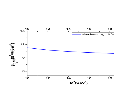
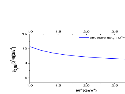
Figure 1: Left: $g_{\Sigma_{b}NB}(Q^{2}=0)$ as a function of the Borel mass $M^{2}$ at average values of continuum thresholds. Right: $g_{\Sigma_{b}NB}(Q^{2}=0)$ as a function of the Borel mass $M^{\prime^{2}}$ at average values of continuum thresholds.

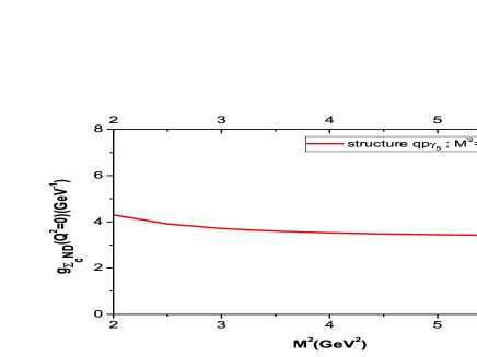
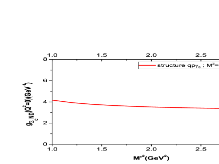
Figure 2: The same as figure 1 but for $g_{\Sigma_{c}ND}(Q^{2}=0)$.

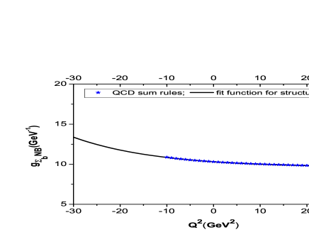
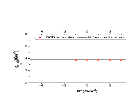
Figure 3: Left: $g_{\Sigma_{b}NB}(Q^{2})$ as a function of $Q^{2}$ at average values of the continuum thresholds and Borel mass parameters. Right: $g_{\Sigma_{c}ND}(Q^{2})$ as a function of $Q^{2}$ at average values of the continuum thresholds and Borel mass parameters.

Subsequent to the determination of the auxiliary parameters, their working windows together with the other input parameters are used to ascertain the dependency of the strong coupling form factors on $Q^{2}$. From our analysis we observe that the dependency of the strong coupling form factors on $Q^{2}$ is well characterized by the following fit function:

$$g_{\Sigma_{b}NB[\Sigma_{c}ND]}(Q^{2})=c_{1}\exp\Big{[}-\frac{Q^{2}}{c_{2}}\Big{]}+c_{3}.$$ (14)

The values of the parameters $c_{1}$, $c_{2}$ and $c_{3}$ for $\Sigma_{b}NB$ and $\Sigma_{c}ND$ can be seen in tables 2 and 3, respectively. Considering the average values of the continuum thresholds and Borel mass parameters we demonstrate the variation of the strong coupling form factors with respect to $Q^{2}$ for the QCD sum rules as well as the fitting results in figure 3. The figure indicates the truncation of the QCD sum rules at some points at negative values of $Q^{2}$. It can be seen from the figure that there is a good consistency among the results obtained from the QCD sum rules and fit function up to these points. The fit function is used to determine the value of the strong coupling constant at $Q^{2}=-m_{B[D]}^{2}$, and the results are presented in table 4. The presented errors in these results originate from the uncertainties of the input parameters together with the uncertainties coming from the determination of the working regions of the auxiliary parameters.

$$\begin{array}[]{|c|c|c|c|}\hline\cr\hline\cr\mbox{Parameters}&c_{1}(\mbox{GeV${}^{-1}$})&c_{2}(\mbox{GeV${}^{2}$})&c_{3}(\mbox{GeV${}^{-1}$})\\ \hline\cr\mbox{Values}&0.72\pm 0.20&18.03\pm 4.87&9.60\pm 2.88\\ \hline\cr\hline\cr\end{array}$$

Table 2: Parameters appearing in the fit function of the coupling form factor for $\Sigma_{b}NB$ vertex.

$$\begin{array}[]{|c|c|c|c|}\hline\cr\hline\cr\mbox{Parameters}&c_{1}(\mbox{GeV${}^{-1}$})&c_{2}(\mbox{GeV${}^{2}$})&c_{3}(\mbox{GeV${}^{-1}$})\\ \hline\cr\mbox{Values}&-0.006\pm 0.002&-6.78\pm 1.89&3.79\pm 1.02\\ \hline\cr\hline\cr\end{array}$$

Table 3: Parameters appearing in the fit function of the coupling form factor for $\Sigma_{c}ND$ vertex.

$$\begin{array}[]{|c|c||c|c|}\hline\cr\hline\cr\mbox{Coupling Constants}&g_{\Sigma_{b}NB}(Q^{2}=-m_{B}^{2})(\mbox{GeV${}^{-1}$})&g_{\Sigma_{c}ND}(Q^{2}=-m_{D}^{2})(\mbox{GeV${}^{-1}$})\\ \hline\cr\mbox{Values}&12.96\pm 3.49&3.78\pm 1.06\\ \hline\cr\hline\cr\end{array}$$

Table 4: Values of the coupling constants $g_{\Sigma_{b}NB}$ and $g_{\Sigma_{c}ND}$.

To sum up, in this work, the strong coupling constants among the heavy bottom spin–1/2 $\Sigma_{b}$ baryon, nucleon and $B$ meson as well as the heavy charmed spin–1/2 $\Sigma_{c}$ baryon, nucleon and $D$ meson, namely $g_{\Sigma_{b}NB}$ and $g_{\Sigma_{c}ND}$, have been calculated in the framework of the three-point QCD sum rules. The obtained results can be applied in the analysis of the related experimental results at LHC. The predictions can also be used in the bottom and charmed mesons clouds description of the nucleon that may be applied for the explanation of the exotic events observed by different experiments. These results may also serve the purpose of analyzing of the results of heavy ion collision experiments like $\overline{P}ANDA$ at FAIR. The obtained results may also come in handy in the determinations of the changes in the masses, decay constants and other parameters of the $B$ and $D$ mesons in nuclear medium.

4 Acknowledgment

This work has been supported in part by the Scientific and Technological Research Council of Turkey (TUBITAK) under the research project 114F018.

References

• [1] F. O. DurΓ£es, M. Nielsen, Phys. Lett. B 658, 40 (2007).
• [2] D. Ebert, R. N. Faustov, V. O. Galkin, Phys. Rev. D 72, 034026 (2005).
• [3] A. Faessler, Th. Gutsche, M. A. Ivanov, J. G. KΓΆrner, V. E. Lyubovitskij, D. Nicmorus, and K. Pumsa-ard, Phys. Rev. D 73, 094013 (2006).
• [4] F. S. Navarra, M. Nielsen, Phys. Lett. B 443, 285 (1998).
• [5] K. Azizi, M. Bayar, A. Ozpineci, Phys. Rev. D 79, 056002 (2009).
• [6] Z.-G. Wang, Eur. Phys. J. A 44, 105 (2010); Phys. Rev. D 81, 036002 (2010).
• [7] A. Khodjamirian, Ch. Klein, and Th. Mannel, and Y.-M. Wang, J. High Energy Phys. 09 (2011) 106.
• [8] E. Hernandez, J. Nieves, Phys. Rev. D 84, 057902 (2011).
• [9] K. Azizi, M. Bayar, Y. Sarac and H. Sundu, Phys. Rev. D 80, 096007 (2009).
• [10] T. Gutsche, M. A. Ivanov, J. G. Korner, V. E. Lyubovitskij, and P. Santorelli, arXiv:1410.6043 (2014).
• [11] K. Azizi, Y. Sarac and H. Sundu, Phys. Rev. D 90, 114011 (2014).
• [12] K. Azizi, N. Er, H. Sundu, Eur. Phys. J. C 74, 3021 (2014).
• [13] A. Kumar, Adv. High Energy Phys. 2014, 549726 (2014).
• [14] Z.-G. Wang and T. Huang, Phys. Rev. C 84, 048201 (2011).
• [15] A. Hayashigaki, Phys. Lett. B 487, 96 (2000).
• [16] L. J. Reinders, H. Rubinstein and S. Yazaki, Phys. Rep. 127, 1 (1985).
• [17] K. A. Olive et al. (Particle Data Group), Chin. Phys. C 38, 090001 (2014).
• [18] A. Khodjamirian, β€œB and D Meson Decay Constant in QCD,” in Proceeding of 3rd Belle Analysis School, 22, 2010 (KEK, Tsukuba, Japan, 2010).
• [19] B. I. Eisenstein et al. (CLEO Collab.), Phys. Rev. D78, 052003 (2008).
• [20] K. Azizi, N. Er, Eur. Phys. J. C 74, 2904 (2014).
• [21] B. L. Ioffe, Prog. Part. Nucl. Phys. 56, 232 (2006).
• [22] V. M. Belyaev, B. L. Ioffe, Sov. Phys. JETP 57, 716 (1983); Phys. Lett. B 287, 176 (1992).