Discrete-Time Models for
Implicit Port-Hamiltonian Systems

Abstract

Implicit representations of finite-dimensional port-Hamiltonian systems are studied from the perspective of their use in numerical simulation and control design. Implicit representations arise when a system is modeled in Cartesian coordinates and when the system constraints are applied in the form of additional algebraic equations (the system model is in a differential-algebraic equation form). Such representations lend themselves better to sample-data approximations. Given an implicit representation of a port-Hamiltonian system it is shown how to construct a sampled-data model that preserves the port-Hamiltonian (PH) structure under sample and hold.

1 Introduction

The class of Hamiltonian systems has a prominent role in many disciplines. It was recently extended in [6] to include open systems, i.e. systems that interact with the environment via a set of inputs and outputs (called ports), giving rise to PH systems. Such extended models immediately reveal the passive properties of the underlying systems, making them particularly well suited for designing passivity-based control (PBC) laws. Two types of model representations of Hamiltonian systems are in widespread use: the explicit representation stated in the form of an ordinary differential equation (ODE) on an abstract manifold [28, 29, 25, 26] and the implicit representation stated in the form of a differential-algebraic equation (DAE) usually evolving in a Euclidean space [4]. While explicit representations are usually preferred in the context of analytical mechanics; see [1, 8, 19], the implicit DAEs models lend themselves better for numerical computations as they lead to simpler expressions for the Hamiltonian functions. The formal relations between the two representations and their equivalence can be established if the system’s configuration space is regarded as an embedded submanifold of the Euclidean space; see [4] for a full development.

Of principal interest here will be the construction of sampled-data (discrete-time) models of PH systems that best approximate their continuous-time counterparts. Sampled-data models are important in digital control implementations and permit for simpler design of PBC laws directly in discrete time. In this context, the notion of “best approximation” deserves clarification.

For linear systems, exact sampled-data models can be constructed by requiring that the solutions of the sampled-data and continuous-time systems coincide at the discretization points. Point-wise model matching is usually impossible in the case of nonlinear systems short of explicit derivation of analytical expressions for their solutions. For general dynamic systems, it is thus the choice of an integration method for generating an approximate solution (like Euler or Runge-Kutta) whose precision relates to the compromise between complexity and order of approximation of the given continuous-time system by its sampled-data counterpart. In the special case of Hamiltonian systems, structure preservation is usually the main criterion for choosing a numerical method; see, e.g., [11] for more details on structure-preserving numerical schemes. Structure-preserving methods guarantee accuracy in long-horizon simulations.

It is known that autonomous Hamiltonian systems conserve two quantities: the Hamiltonian function $H$ (i.e., the energy or storage function) and a certain two-form $\omega$, called the symplectic form. Numerical integration algorithms can either conserve $H$ [14, 15] or $\omega$ [27], but not both. Conservation of $\omega$ is usually preferred over conservation of $H$ as the symplectic form unambiguously defines the class of Hamiltonian vector fields; see Theorem 3 and Remark 1.

Contribution

Adopting a symplectic-form preserving approach, a sampled-data model for a given continuous-time PH system in developed here. The approach employs implicit representations of PH systems as the latter lead to simpler expressions for the Hamiltonian functions. Specifically, the Hamiltonian functions arising from implicit representations lend themselves well to the application of flow-splitting numerical integration methods; see [27] for a splitting method that applies to autonomous Hamiltonian systems (Hamiltonian systems without ports). Additionally, the discrete-time modeling approach presented here preserves passivity of PH systems (Theorem 12). The passive structure is preserved in the sense that the discrete model is the exact representation of another, possibly non affine, continuous-time PH system which, up to an approximation error of order two with respect to the sampling interval, has the same storage function $H$ and the same output function $y$.

Paper structure

Section 2 introduces the implicit representations of PH systems. This section recalls the results from [4] and serves mainly to introduce the notation and to state the main assumptions (1 and 2). Also, the definition of PH systems is extended to the case of non affine control systems. Splitting and symplectic integration methods for autonomous systems are recalled in § 3. Discrete-time models for implicit PH systems based on vector splitting methods are developed in § 4 and their asymptotic properties are analyzed. An illustrative example is provided confirming the findings.

2 Implicit representations of port-Hamiltonian systems

We begin this section by defining the configuration and phase spaces of Hamiltonian systems in implicit form. Conservative properties are also discussed. Similarly to the case of explicit representations of Hamiltonian systems, both the Hamiltonian function and the symplectic two-form of the implicit representation are invariant under the flow of the system. Following [6], input and output ports are added to the implicit representation, insuring passivity of the resulting PH system. Finally, we extend the definition of PH to the the case of non affine control systems. This will be needed when performing backward error analysis later in § 4 since time discretization entails the loss of affinity.

2.1 The configuration space

The class of systems considered here is restricted to mechanical finite-dimensional systems with scleronomic constraints that evolve in continuous time. Systems of this type typically consist of $M$ rigid bodies held together as one structure by the action of constraint forces. The position of each of the rigid bodies can be unambiguously described in terms of the position of its center of mass and its orientation in space. The configuration space of a spatial system as a whole can thus be viewed as a subset, $\mathbb{G}$, of a Cartesian space of dimension $n=6M$ that is expressed in terms of smooth, independent constraint functions $g:\mathbb{R}^{n}\to\mathbb{R}^{k}$, with $k\leq n$, as the level set

$$\mathbb{G}:=g^{-1}(0)=\left\{r\in\mathbb{R}^{n}\;|\;g(r)=0\right\}$$ (1)

where $g^{-1}(0)$ is the inverse image of $0\in\mathbb{R}^{k}$. Functional independence of the constraints is expressed in terms of the following rank condition.

Assumption 1.

The rank of $g$ is equal to $k$ at all points of the set $g^{-1}(0)$.

Recalling that the rank of a mapping is the rank of its tangent map (pushforward by $g$), then in any coordinates, the condition requires that the Jacobian $G:=\left\{\partial g_{i}/\partial r_{j}\right\}_{ij}$ has full rank, i.e., $\mathop{\operator@font rank}\nolimits(G)=k$ at every point of $g^{-1}(0)$. The value $0\in\mathbb{R}^{k}$ is then called a regular value of $g$, the level set $g^{-1}(0)$ is a regular level set of $g$, and $g$ is said to be a defining map for $g^{-1}(0)$; see [16], p. 113-114. It hence follows that $\mathbb{G}$ can be given the differentiable structure of a closed embedded submanifold of $\mathbb{R}^{n}$; see [16], Corollary 5.24, p. 114. The Constant-Rank Level Set Theorem ([16], Theorem 5.22, p. 113), further specifies its dimension as $o=n-k$.

Because $\mathbb{G}$ is an embedded submanifold, it can also be regarded as an abstract $o$-dimensional manifold with local coordinates $q$ (called generalized coordinates in mechanics). It is then also possible to exhibit an injective inclusion map: $\imath:\mathbb{G}\hookrightarrow\mathbb{R}^{n}$ (embedding), with $\mathop{\operator@font rank}\nolimits(\imath)=\dim\mathbb{G}$, which is a homeomorphism onto the image $\imath(\mathbb{G})\subset\mathbb{R}^{n}$ and such that $\imath(q)=r$ and $g\circ\imath\equiv 0$. This inclusion serves as a map between local coordinates $q$ and global Cartesian coordinates $r$.

2.2 Hamiltonian equations

Let $T^{*}\mathbb{G}$ be the cotangent bundle of $\mathbb{G}$ and let $\left\{q^{i},{\hat{p}}_{i}\right\}$ be local coordinates. A system is said to be Hamiltonian if its trajectories are integral curves of the Hamiltonian vector field $D_{\hat{H}}:T^{*}\mathbb{G}\to T(T^{*}\mathbb{G})$,

$$D_{{\hat{H}}}=\frac{\partial{\hat{H}}}{\partial{\hat{p}}_{i}}\frac{\partial}{\partial q^{i}}-\frac{\partial{\hat{H}}}{\partial q^{i}}\frac{\partial}{\partial{\hat{p}}_{i}}\;,$$

where ${\hat{H}}:T^{*}\mathbb{G}\to\mathbb{R}$ is the sum of the system’s kinetic and potential energies $\hat{K}:T^{*}\mathbb{G}\to\mathbb{R}$ and $\hat{V}:\mathbb{G}\to\mathbb{R}$, respectively; see [1] for more details and a coordinate-free definition.

The implicit model for a Hamiltonian system is defined as follows. Let $T^{*}\mathbb{R}^{n}$ be the cotangent bundle of $\mathbb{R}^{n}$ and let $\left\{r^{i},p_{i}\right\}$ be global coordinates. The implicit Hamiltonian vector field takes the form

$$X_{H,g}=D_{H}-\lambda_{j}\frac{\partial g^{j}}{\partial r^{i}}\frac{\partial}{\partial p_{i}}\;,\quad g=0\;,$$ (2)

with

$$D_{H}=\frac{\partial H}{\partial p_{i}}\frac{\partial}{\partial r^{i}}-\frac{\partial H}{\partial r^{i}}\frac{\partial}{\partial p_{i}}$$ (3)

the unconstrained part of the Hamiltonian vector field and $H:T^{*}\mathbb{R}^{n}\to\mathbb{R}$ is again the sum of the kinetic and potential energies, but expressed in global coordinates. That is, $K:T^{*}\mathbb{R}^{n}\to\mathbb{R}$ and $V:\mathbb{R}^{n}\to\mathbb{R}$; see [11, 27, 3] for details on the derivation of this equation. The vector field unravels as the DAE system

$$\dot{r} =\nabla_{p}H(r,p)\;,\quad\dot{p}=-\nabla_{r}H(r,p)-G(r)^{\top}\lambda$$ (4a)

$$0 =g(r)\;.$$ (4b)

By applying $X_{H,g}$ to both sides of the constraint equations $g^{j}=0$, one obtains the so-called hidden constraints

$$f^{j}:=X_{H,g}(g^{j})=\frac{\partial H}{\partial p_{i}}\frac{\partial g^{j}}{\partial r^{i}}=0\;.$$ (5)

Thus, the system evolves on the closed submanifold

$$L\mathbb{G}=\left\{(r,p)\in T^{*}\mathbb{R}^{n}\;|\;g(r)=0,f(r,p)=0\right\}$$ (6)

and we have $X_{H,g}:L\mathbb{G}\to T(L\mathbb{G})$. A more rigorous construction of the phase space $L\mathbb{G}$ is given in [4], where it is regarded as an embedding of $T^{*}\mathbb{G}$ in $T^{*}\mathbb{R}^{n}$. The map ${\hat{p}}\mapsto p$ as well as the formal relation between ${\hat{H}}$ and $H$ can also be found in [4].

The Lagrange multipliers $\lambda_{j}$ are defined implicitly by (2). Precisely, application of $X_{H,g}$ to the hidden constraints makes $\lambda_{j}$ appear:

$$X_{H,g}(f^{l})=D_{H}(f^{l})-\lambda_{j}\frac{\partial g^{j}}{\partial r^{i}}\frac{\partial f^{l}}{\partial p_{i}}=0\;.$$ (7)

Thus, if the matrix

$$\left\{\frac{\partial g^{j}}{\partial r^{i}}\frac{\partial f^{l}}{\partial p_{i}}\right\}_{jl}=\left\{\frac{\partial g^{j}}{\partial r^{i}}\frac{\partial^{2}H}{\partial p_{i}\partial p_{m}}\frac{\partial g^{l}}{\partial r^{m}}\right\}_{jl}$$ (8)

is non-singular on $L\mathbb{G}$, then there are unique $\lambda_{j}$ satisfying (7) and forcing the integral curves to stay on $L\mathbb{G}$.

Assumption 2.

The Hessian matrix $\left\{\partial^{2}H(r,p)/\partial p_{i}\partial p_{j}\right\}_{ij}$ is positive definite for all $(r,p)\in T^{*}\mathbb{R}^{n}$ so $H(r,p)$ is convex in $p$.

This assumption, satisfied by most mechanical systems, together with Assumption 1 ensures that the matrix in (8) is invertible and the system is well defined. In mechanical systems, $\lambda$ is the covector of constraint forces that insure satisfaction of the constraints during the evolution of the system.

2.3 Energy conservation and symplecticity

It is well known that the flows generated by Hamiltonian vector fields in explicit form preserve the Hamiltonian function, i.e. the total energy of the system is conserved during the evolution of the system [32, 23, 24]. As the explicit and implicit system representations are equivalent, the conservation also holds for the implicit Hamiltonian vector field (2), as is easily confirmed by computing the Lie derivative of $H$ along the flow generated by $X_{H,g}$ [11]. Indeed,

$$\mathcal{L}_{X_{H,g}}H=X_{H,g}(H)=D_{H}(H)-\lambda_{j}\frac{\partial g^{j}}{\partial r^{i}}\frac{\partial H}{\partial p_{i}}=\lambda_{j}f^{j}\;,$$ (9)

where the third equality holds because $D_{H}(H)=0$ and because of the definition of $f$ given in (5). Eq. (9) shows that $\mathcal{L}_{X_{H,g}}H\big{|}_{L\mathbb{G}}=0$ (cf. Eq. (6)), so $H$ remains constant along the system trajectories.

It is also well known that, besides the 0-form $H$, Hamiltonian flows preserve a certain 2-form called the symplectic form. In the case of implicit representations the symplectic form is given by the formula

$$\omega:=\mathrm{d}r^{i}\wedge\mathrm{d}p_{i}\;,$$ (10)

which acts on vectors of $T(T^{*}\mathbb{R}^{n})$, with Einstein’s summation convention implied.

Definition 1.

A differentiable mapping $\phi:T^{*}\mathbb{R}^{n}\to T^{*}\mathbb{R}^{n}$ is called symplectic if

$$\phi^{*}\omega=\omega\;.$$ (11)

Here, $\phi^{*}$ denotes the pull-back map associated with $\phi$, defined by

Definition 2.

Let $\phi:\mathcal{M}_{1}\rightarrow\mathcal{M}_{2}$ be a smooth map of manifolds and let $p\in\mathcal{M}_{1}$. The pull-back map $\phi^{*}:T^{*}_{\phi(p)}\mathcal{M}_{2}\rightarrow T^{*}_{p}\mathcal{M}_{2}$ associated with $\phi$ is a dual map to the push-forward map $\phi_{*}$ and is characterized by

$$\langle\phi^{*}\xi,X\rangle=\langle\xi,\phi_{*}X\rangle\ \text{ for }\ \xi\in T^{*}_{\phi(p)}\mathcal{M}_{2},\ X\in T_{p}\mathcal{M}_{1}\;.$$

The application of this definition permits to re-write (11) in the equivalent form

$$\omega(\phi_{*}\xi,\phi_{*}\eta)=\omega(\xi,\eta)\quad\text{for all }\xi,\eta\in T(T^{*}\mathbb{R}^{n})\;.$$ (12)

The conservation of $\omega$ along $X_{H,g}$ can be established by showing that the Lie derivative $\mathcal{L}_{X_{H,g}}\omega$ is equal to zero, the demonstration bearing similarity to that of the conservation of $H$; see [4] for the explicit derivation. Here, we cite the result

Theorem 3.

[11, 17] Let $H$ be twice continuously differentiable. The flow $\phi_{t}:L\mathbb{G}\to L\mathbb{G}$ of $X_{H,g}$ governed by (2) is a symplectic transformation on $L\mathbb{G}$, i.e.,

$$\phi_{t}^{*}\omega=\omega$$

for every $t$ for which $\phi_{t}$ is defined.

Remark 1.

The converse statement, that every symplectic flow $\phi_{t}$ solves Hamilton’s equations for some $H$, is also true, so symplecticity is a characteristic property of Hamiltonian systems [1]. This does not translate to the case of energy conservation, i.e., while every Hamiltonian system conserves energy, not every energy-conserving system is Hamiltonian.

2.4 port-Hamiltonian systems

In the presence of external forces and dissipation it is convenient to represent (2) as an input-output system equipped with a pair of port variables $(u,y)$, giving rise to a PH system; see [20, 32, 23] for the original definition as stated with respect to Hamiltonian systems in explicit form. Extending on this definition the Hamiltonian systems in implicit form, a port-Hamiltonian system is described in terms of the vector field $X_{H,u,g}:L\mathbb{G}\times(\mathbb{R}^{m})^{*}\to T(L\mathbb{G})$:

$$X_{H,u,g}=D_{H}+\left(u_{l}U\indices{{}_{i}^{l}}-\lambda_{j}\frac{\partial g^{j}}{\partial r^{i}}\right)\frac{\partial}{\partial p_{i}}\;,\quad g=0\;,$$ (13)

with $u\in(\mathbb{R}^{m})^{*}$ defined as the controlled or input variable, $y\in\mathbb{R}^{m}$ is defined as the output variable that satisfies

$$y^{l}=U\indices{{}_{i}^{l}}\frac{\partial H}{\partial p_{i}}$$ (14)

and where $U\indices{{}_{i}^{l}}$ are maps from $\mathbb{R}^{n}$ to $\mathbb{R}$.

The vector field (13) and the output unravel as the DAE system

$$\dot{r} =\nabla_{p}H(r,p)\;,\quad\dot{p}=-\nabla_{r}H(r,p)-G(r)^{\top}\lambda+U(r)u$$

$$y =U(r)^{\top}\nabla_{p}H(r,p)$$

$$0 =g(r)\;.$$

By analogy with the results described in Sec. 2.2, one can determine the Lagrange multipliers $\lambda$ explicitly. The constraints $f^{a}=0$ imply that

$$X_{H,u,g}(f^{a})=D_{H}(f^{a})+u_{l}U\indices{{}_{i}^{l}}\frac{\partial f^{a}}{\partial p_{i}}-\lambda_{j}\frac{\partial g^{j}}{\partial r^{i}}\frac{\partial f^{a}}{\partial p_{i}}=0\;,$$ (15)

from where it follows that, as long as (8) is non-singular, there are unique $\lambda_{j}$ (in general dependent on $u$ as well as on $r$ and $p$) such that $X_{H,u,g}(f^{a})=0$ and such that the integral curve stays on $L\mathbb{G}$.

It can be readily seen that an implicit PH system described by (13) no longer preserves $H$. The Lie derivative of $H$ is now

$$\mathcal{L}_{X_{H,u,g}}(H)=X_{H,u,g}(H)=D_{H}(H)+u_{l}U\indices{{}_{i}^{l}}\frac{\partial H}{\partial p_{i}}-\lambda_{j}\frac{\partial g^{j}}{\partial r^{i}}\frac{\partial H}{\partial p_{i}}=u_{l}y^{l}-\lambda_{j}f^{j}\;,$$

which establishes the power balance

$$\mathcal{L}_{X_{H,u,g}}H\big{|}_{L\mathbb{G}}=u_{l}y^{l}\;.$$ (16)

Since the product $u_{l}y^{l}$ is equal to the rate of change in energy, we say that $(u,y)$ is a power-conjugated pair of port variables. If, in addition, the restriction of $H$ to $L\mathbb{G}$ is bounded from below, i.e., if the image of $L\mathbb{G}$ under $H$ is bounded from below, then  (13) is called passive, or more precisely, lossless. Boundedness of $H$ can be easily assessed using the following proposition.

Proposition 4.

[4] If the potential energy $V$ is lower semi-continuous and $\mathbb{G}$ is compact, then $H$ restricted to $L\mathbb{G}$ is bounded from below (hence, the vector field (13) describes a lossless system).

With the inclusion of the control variable $u$, it can no longer be expected that the flow of (13) be symplectic. Indeed, it is not hard to see that the Lie derivative of $\omega$ along $X_{H,u,g}$ is in general different from zero.

Proposition 5.

[4] The Lie derivative of $\omega$ (10) along (13) and restricted to $L\mathbb{G}$ satisfies

$$\mathcal{L}_{X_{H,u,g}}\omega\big{|}_{L\mathbb{G}}=\mathrm{d}r^{i}\wedge\mathrm{d}(u_{l}U\indices{{}_{i}^{l}})\;.$$ (17)

Example: A double planar pendulum

Let us recall an example from [4], on which we will elaborate when discussing sampled-data models.

Consider the model of a double planar pendulum shown in Fig. 1 that comprises a pair of point masses $m_{a}$ and $m_{b}$ whose coordinate positions are $r^{a}=(r^{a_{x}},r^{a_{y}})$ and $r^{b}=(r^{b_{x}},r^{b_{y}})$, respectively. The massless bars are of fixed lengths $l_{a}$ and $l_{b}$ which gives rise to the two holonomic constraints:

$$g^{1}(r)=\|r^{a}\|^{2}-l_{a}^{2}=0\;,\quad g^{2}(r)=\|r^{\delta}\|^{2}-l_{b}^{2}=0$$ (18)

with $r:=(r^{a},r^{b})\in\mathbb{R}^{n}$, $n=4$, $k=2$, $r^{\delta}:=r^{b}-r^{a}$. The rank of the constraint Jacobian is full as

$$\mathop{\operator@font rank}\nolimits G(r)=\mathop{\operator@font rank}\nolimits\begin{pmatrix}r^{a_{x}}&r^{a_{y}}&0&0\\ -r^{\delta_{x}}&-r^{\delta_{y}}&r^{\delta_{x}}&r^{\delta_{y}}\end{pmatrix}=k$$ (19)

for all $r\in\mathbb{G}$. Therefore, $0$ is a regular value of $g$ and $\mathbb{G}$ is an embedded submanifold of $\mathbb{R}^{4}$.

The total energy is

$$H(r,p)=\frac{1}{2}p^{\top}M^{-1}p+\mathrm{bar}{g}(m_{a}r^{a_{y}}+m_{a}r^{a_{y}})\;,$$ (20)

where $M:=\begin{pmatrix}m_{a}\mathbf{I}_{n}&\mathbf{0}_{n}\\ \mathbf{0}_{n}&m_{b}\mathbf{I}_{n}\end{pmatrix}$ and $\mathrm{bar}{g}$ is the standard gravity.

Substituting (18) and (20) in (4) gives

$$\dot{r}^{a} =m_{a}^{-1}p_{a}\;,\quad\dot{r}^{b}=m_{b}^{-1}p_{b}$$ (21a)

$$\begin{pmatrix}\dot{p}_{a_{x}}\\ \dot{p}_{a_{y}}\\ \dot{p}_{b_{x}}\\ \dot{p}_{b_{y}}\end{pmatrix} =-\begin{pmatrix}0\\ \mathrm{bar}{g}m_{a}\\ 0\\ \mathrm{bar}{g}m_{b}\end{pmatrix}-2\begin{pmatrix}r^{a_{x}}&-r^{\delta_{x}}\\ r^{a_{y}}&-r^{\delta_{y}}\\ 0&r^{\delta_{x}}\\ 0&r^{\delta_{y}}\end{pmatrix}\begin{pmatrix}\lambda_{1}\\ \lambda_{2}\end{pmatrix}$$ (21b)

which, together with (18), constitutes a set of DAEs describing the motion of the double pendulum in implicit form. The multipliers $\lambda_{1}$ and $\lambda_{2}$ are the magnitudes of the tension along the two bars.

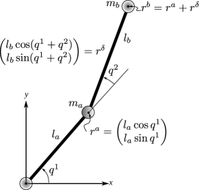
Fig. 1: A double planar pendulum, a simple Hamiltonian system.

Now, assume that the double pendulum is actuated by application of torques $u_{1}$ and $u_{2}$ to the joints that correspond to the angles $q^{1}$ and $q^{2}$, respectively. The resulting linear forces are then $U^{1}u_{1}$ and $U^{2}u_{2}$ with

$$U^{1}:=\{U\indices{{}_{i}^{1}}\}_{i}=\begin{pmatrix}-r^{a_{y}}\\ r^{a_{x}}\\ 0\\ 0\end{pmatrix}\frac{1}{l_{a}^{2}}\quad\text{and}\quad U^{2}:=\{U\indices{{}_{i}^{2}}\}_{i}=\begin{pmatrix}r^{\delta_{y}}\\ -r^{\delta_{x}}\\ -r^{\delta_{y}}\\ r^{\delta_{x}}\end{pmatrix}\frac{1}{l_{b}^{2}}-U^{1}\;.$$ (22)

The manifold defined by (18) is compact and the potential energy is continuous, which confirms that the double pendulum is passive with passive outputs $y^{l}=U\indices{{}_{i}^{l}}\frac{\partial H}{\partial p_{i}}=U\indices{{}_{i}^{l}}\dot{r}^{i}$.

An explicit model for the double pendulum as an ODE can be derived by choosing the generalized coordinates on $\mathbb{G}$ as $q^{1}\in(-\pi,\pi)$ and $q^{2}\in(-\pi,\pi)$, as motivated by Fig. 1. The associated embedding $r=\imath(q)$ satisfying $g\circ\imath\equiv 0$ is readily exhibited as

$$\begin{pmatrix}r^{a_{x}}\\ r^{a_{y}}\\ r^{b_{x}}\\ r^{b_{y}}\end{pmatrix}=\begin{pmatrix}l_{a}\cos q^{1}\\ l_{a}\sin q^{1}\\ l_{a}\cos q^{1}+l_{b}\cos q^{\mathrm{t}}\\ l_{a}\sin q^{1}+l_{b}\sin q^{\mathrm{t}}\end{pmatrix}\;,\quad q^{\mathrm{t}}:=q^{1}+q^{2}\;.$$ (23)

In local coordinates, the total energy is

$${\hat{H}}(q,{\hat{p}})=\frac{1}{2}{\hat{p}}^{\top}\hat{M}(q)^{-1}{\hat{p}}+\mathrm{bar}{g}\left(m_{\mathrm{t}}l_{a}\sin q^{1}+m_{b}l_{b}\sin q^{\mathrm{t}}\right)\;.$$ (24)

with

$$\hat{M}(q)=\begin{pmatrix}m_{\mathrm{t}}l_{a}^{2}+m_{b}l_{b}^{2}+2m_{b}l_{a}l_{b}\cos q^{2}\!&\!m_{b}l_{b}^{2}+m_{b}l_{a}l_{b}\cos q^{2}\\ m_{b}l_{b}^{2}+m_{b}l_{a}l_{b}\cos q^{2}&m_{b}l_{b}^{2}\end{pmatrix}$$

The motion of the system is described by

$$\dot{q}=\hat{M}(q)^{-1}{\hat{p}}\;,\;\dot{{\hat{p}}}=-\nabla_{q}V(q)-\nabla_{q}\left(\frac{1}{2}{\hat{p}}^{\top}\hat{M}(q)^{-1}{\hat{p}}\right)+u$$ (25)

(see [4] for more details).

Two representations for the same system were derived, one in the form of an ODE (25) and the other as a DAE (21). The main point of this example can be summarized in the following remark.

Remark 2.

The implicit DAE representation of the Hamiltonian systems renders a separable Hamiltonian function (20), i.e. the kinetic energy does not depend on $r$ and the inertia matrix $M$ is a constant diagonal matrix. Moreover, the potential energy is linear, which results in a constant potential energy gradient. On the other hand it is easily verified that the explicit Hamiltonian representation does not share such fortunate properties. The explicit Hamiltonian is no longer separable and the inertia matrix depends on the generalized coordinates $q$.

The a cost of a simpler Hamiltonian function is the higher dimensional implicit model representation and the appearance of the Lagrange multipliers. As will soon be seen, however, implicit representations are particularly advantageous for the purposes of system discretization.

2.5 Non affine port-Hamiltonian systems

It was assumed in (13) that the control variables enter the vector field affinely. Many physical systems exhibit this property so, from a modeling point of view, this assumption is not too restrictive. However, for the purpose of performing backward error analysis in § 4, we will need to consider PH systems for which the control might enter in a non affine way. Motivated by the fact that $\mathcal{L}_{X_{H,u,g}}\omega\big{|}_{L\mathbb{G}}=0$ when $u\equiv 0$, we propose the following extended definition of a PH system.

Definition 6.

A controlled vector field $X:L\mathbb{G}\times(\mathbb{R}^{m})^{*}\to T(L\mathbb{G})$ is said to be port-Hamiltonian if $u\equiv 0$ implies that the generated flow is symplectic.

Passivity of a non affine port-Hamiltonian system can be established by redefining the passive output.

Lemma 7.

A (not necessarily affine) smooth PH system described by a vector field $X$ can always be decomposed as $X=X_{0}+u_{l}Z^{l}$, where $X_{0}:L\mathbb{G}\to T(L\mathbb{G})$ is a Hamiltonian vector field and $Z^{l}:L\mathbb{G}\times(\mathbb{R}^{m})^{*}\to T(L\mathbb{G})$ are the input vector fields. Hence, $X$ satisfies the power balance $X(H)=u_{l}y^{l}$ for some real-valued function $H$ and real-valued output functions $y^{l}=Z^{l}(H)$. (The output functions may now depend directly on $u$ as well as on $r$ and $p$.)

Proof.

Following [18], we first show that a smooth control vector field can be split into a drift and a set of vector fields having $u$ factored out. Let us define the drift $X_{0}$ as $X_{0}(x)=X(x,0)$ and let us define the vector fields $W^{l}$ by the equations

$$W^{l}(\alpha)=\frac{\partial}{\partial u_{l}}\Big{(}X(\alpha)\Big{)}\quad\text{for all }\alpha\in\mathcal{C}^{\infty}(L\mathbb{G},\mathbb{R})\;.$$

It follows from the chain rule that

$$u_{l}W^{l}(x,\theta u)(\alpha)=\frac{\mathrm{d}}{\mathrm{d}\theta}\Big{(}X(x,\theta u)\Big{)}(\alpha)\;.$$

Upon integration on both sides of the equation we arrive at

$$u_{l}\int_{0}^{1}W^{l}(x,\theta u)(\alpha)\mathrm{d}\theta=X(x,\theta u)(\alpha)\Big{|}_{0}^{1}=X(x,u)(\alpha)-X_{0}(x)(\alpha)\;.$$

Therefore, we have

$$X=X_{0}+u_{l}Z^{l}\;,$$ (26)

where the input vector fields $Z^{l}$ are defined by

$$Z^{l}(x,u)(\alpha)=\int_{0}^{1}W^{l}(x,\theta u)(\alpha)\mathrm{d}\theta\quad\text{for all }\alpha\in\mathcal{C}^{\infty}(L\mathbb{G},\mathbb{R})\;.$$

It follows from the hypothesis that $X_{0}$ generates a symplectic flow, so it is a Hamiltonian vector field and satisfies $X_{0}(H)=0$ for some real-valued function $H$. Applying $X$ to $H$ shows that $X(H)=X_{0}(H)+u_{l}Z^{l}(H)=u_{l}y^{l}$ with $y^{l}=Z^{l}(H)$. ∎

Remark 3.

For an affine PH system, the formulae of this lemma recover the output functions (14) with $Z^{l}=U\indices{{}_{j}^{l}}\frac{\partial}{\partial p_{j}}$, that is, $y^{l}=Z^{l}(H)=U\indices{{}_{i}^{l}}\frac{\partial H}{\partial p_{i}}$.

3 Sampled-data models for autonomous Hamiltonian systems

Computing a sampled-data model of a dynamical system basically amounts to computing an approximate solution of the differential equations during a small interval of time. This problem has been studied extensively in the literature of numerical analysis, from which we borrow some results and terminology. In numerical analysis, a sampled-data model is the central component of an integration method or a numerical integrator, up to the point that these terms are used interchangeably.

Mathematical models for sampled-data systems arise in diverse circumstances. In the direct approach to digital control, i.e., as opposed to the emulation of continuous control laws, the design of the controller is performed in discrete time, the designer working directly over a sampled-data model. When designing directly in discrete time, the controller can be directly implemented on a digital device. Also, it is possible to exploit the advantages of switched controls or, e.g., multirate control techniques [21].

Computing the sampled-data model for a given nonlinear system relies on the computation of a solution $\phi_{t}$ of the corresponding ODE or DAE, which is in general impossible to do analytically, so one has to settle for an approximate solution.

When simulating the behavior of dynamic systems, a discrete-time model of the continuous system is also used for computing a numerical solution to the initial-value problem. Many different integration methods (or methods for short) can be found in the literature. Let us first focus on integration methods for autonomous systems and further restrict our attention to one-step methods defined by a transformation

$$\psi_{h}:x_{\alpha}\mapsto x_{\alpha+1}\;,$$

where the constant step-size $h$ is regarded as a parameter of the method. For a given initial condition $x_{0}$ in the phase space, $\psi_{h}$ is applied recursively to generate a discrete flow $x_{1},x_{2},x_{3},\dots$ that approximates the true flow $\phi_{h}(x_{0}),\phi_{2h}(x_{0})$, $\phi_{3h}(x_{0}),\dots$ of a given vector field $X$ at time instants $h,2h,3h,\dots$ In this sense, the map $\psi_{h}$ is a discrete-time approximation of $\phi_{h}$ (or a sampled-data model of $\phi_{h}$).

Definition 8.

A one-step method has order $s$ if the local error satisfies

$$\psi_{h}(x_{0})-\phi_{h}(x_{0})=\mathcal{O}(h^{s+1})\quad\text{as}\quad h\to 0$$ (27)

uniformly in $x_{0}$. A one-step method is said to be consistent if $s\geq 1$.

Let us now discuss some important properties of numerical integrators, like order and symmetry.

3.1 Symplectic methods

If a sampled-data model approximates the discrete time behavior of a Hamiltonian system, one could hope for $\psi_{h}$ to inherit its fundamental qualitative properties: energy conservation and symplecticity. Unfortunately, it is not possible to preserve $H$ and $\omega$ simultaneously, unless $\psi_{h}$ agrees with the exact flow $\phi_{h}$ up to a reparametrization of time [7]. For this reason, one has to choose either in favor of one or the other invariant. Energy conserving methods have received some attention [9, 31, 10, 12, 13], but in light of Remark 1, most of the literature focuses on symplectic integration algorithms (see [11, 17, 5] and references therein). A comparison between both approaches is carried out in [30] for the rigid body.

A theoretical advantage of constructing a symplectic one-step method is that, even though $\psi_{h}$ only approximates $\phi_{h}$ up to the $s$’th order, it coincides exactly (if one disregards convergence issues) with the flow of another Hamiltonian system, a modified Hamiltonian system described by a modified differential equation.

Theorem 9.

[11, p. 352] A symplectic method $\psi_{h}:L\mathbb{G}\to L\mathbb{G}$ for the constrained Hamiltonian system (4) has a modified equation that is locally of the form

$$\dot{r} =+\nabla_{p}\tilde{H}(r,p)\;,\quad\dot{p}=-\nabla_{r}\tilde{H}(r,p)-G(r)^{\top}\tilde{\lambda}$$ (28a)

$$0 =g(r)$$ (28b)

with $\tilde{H}=H+hH_{2}+h^{2}H_{3}+\dots$ Furthermore,

$$\frac{\partial H_{j}(r,p)}{\partial p_{i}}\frac{\partial g^{l}(r)}{\partial r^{i}}=0\;,\quad\text{for all }(r,p)\in L\mathbb{G}\;,$$

all $l=1,\dots,k$ and all $j$. Note that the actual value of the Legendre multipliers $\tilde{\lambda}$ differ in general from those obtained for the original system (4).

In other words, for an initial condition $x_{0}$, $\psi_{h}(x_{0})$ is equal to the solution of (28) at time $t=h$. Note that (27) provides information about the difference between the actual flow $\phi_{h}$ of $X$ and the approximate discrete flow $\psi_{h}$. This is the kind of information that forward error analysis aims at. While certainly useful as an indicator of the quality of the approximation, Eq. (27) only evaluates the behavior of the approximate flow on the first iteration, but says nothing about its long time behavior. From (27) alone we cannot infer anything about the error $x_{\alpha}-\phi_{\alpha h}(x_{0})$ when $\alpha$ is large, so we do not know if errors accumulate or if they average out to zero.

On the other hand, Theorem 9 tells us that if $\psi_{h}$ is symplectic, then there exists a modified continuous system whose flow coincides exactly with the discrete flow generated by $\psi_{h}$. The modified system (28) preserves the Hamiltonian structure of the original system (4) and it is ‘close’ to it in the sense that $\tilde{H}=H+\mathcal{O}(h^{s})$ for a method of order $s$. In other words, a symplectic integration method preserves the original 2-form $\omega$ and a different (but close) Hamiltonian function. This property guaranties that the good behavior of the integration scheme is maintained during many iterations, giving a global nature to the local property (27). This observation is at the center of backward error analysis [11].

3.2 Splitting methods

A practical advantage of symplectic schemes is that they lend themselves well to the application of splitting methods. To illustrate the idea, consider again the unconstrained or, otherwise, explicit Hamiltonian vector field $D_{\hat{H}}$ on an abstract manifold $T^{*}\mathbb{G}$. If the Hamiltonian function is separable, i.e., if it can be written as ${\hat{H}}(q,{\hat{p}})={\hat{H}}_{\mathrm{a}}(q)+{\hat{H}}_{\mathrm{b}}({\hat{p}})$, then the vector field can be spilt into two Hamiltonian vector fields

$$D_{{\hat{H}}_{\mathrm{a}}}=-\frac{\partial{\hat{H}}_{\mathrm{a}}}{\partial q^{i}}\frac{\partial}{\partial{\hat{p}}_{i}}\quad\text{and}\quad D_{{\hat{H}}_{\mathrm{b}}}=\frac{\partial{\hat{H}}_{\mathrm{b}}}{\partial{\hat{p}}_{i}}\frac{\partial}{\partial q^{i}}$$

with $D_{{\hat{H}}}=D_{{\hat{H}}_{\mathrm{a}}}+D_{{\hat{H}}_{\mathrm{b}}}$. Notice that, taken separately, each vector field can be trivially integrated exactly. For $(q_{\alpha},{\hat{p}}_{\alpha})\in T^{*}\mathbb{G}$ (we use the subindex $\alpha$ to refer to an element in a sequence, not a particular coordinate) we have

$$\begin{pmatrix}\dot{q}\\ \dot{{\hat{p}}}\end{pmatrix}=\begin{pmatrix}0\\ -\nabla_{q}{\hat{H}}_{\mathrm{a}}(q)\end{pmatrix}\quad\Longrightarrow\quad\begin{pmatrix}q_{\alpha+1}\\ {\hat{p}}_{\alpha+1}\end{pmatrix}=\begin{pmatrix}q_{\alpha}\\ {\hat{p}}_{\alpha}-h\cdot\nabla_{q}{\hat{H}}_{\mathrm{a}}(q_{\alpha})\end{pmatrix}=\phi_{\mathrm{a},h}\begin{pmatrix}q_{\alpha}\\ {\hat{p}}_{\alpha}\end{pmatrix}$$

and

$$\begin{pmatrix}\dot{q}\\ \dot{{\hat{p}}}\end{pmatrix}=\begin{pmatrix}+\nabla_{p}{\hat{H}}_{\mathrm{b}}({\hat{p}})\\ 0\end{pmatrix}\quad\Longrightarrow\quad\begin{pmatrix}q_{\alpha+1}\\ {\hat{p}}_{\alpha+1}\end{pmatrix}=\begin{pmatrix}q_{\alpha}+h\cdot\nabla_{\hat{p}}{\hat{H}}_{\mathrm{b}}({\hat{p}}_{\alpha})\\ {\hat{p}}_{\alpha}\end{pmatrix}=\phi_{\mathrm{b},h}\begin{pmatrix}q_{\alpha}\\ {\hat{p}}_{\alpha}\end{pmatrix}\;.$$

A first-order symplectic method can be easily constructed by performing the composition

$$\psi_{h}=\phi_{\mathrm{b},h}\circ\phi_{\mathrm{a},h}\;.$$ (29)

Indeed, the maps $\phi_{\mathrm{b},h}$ and $\phi_{\mathrm{a},h}$ are symplectic because they are the exact flows of Hamiltonian vector fields. Since the composition of two symplectic maps is again symplectic, $\psi_{h}$ is symplectic.

Many simple Hamiltonian systems with phase space $T^{*}\mathbb{G}$ are not governed by separable Hamiltonians, so splitting methods cannot be applied directly. However, the Hamiltonian function of many mechanical systems becomes separable if the phase space is embedded in $T^{*}\mathbb{R}^{n}$ (see, e.g., Remark 2). An interesting symplectic method that is particularly well suited for this class of systems was proposed in [27]. Roughly speaking, the idea is to compute a symplectic method for the unconstrained Hamiltonian vector field $D_{H}:T^{*}\mathbb{R}^{n}\to T(T^{*}\mathbb{R}^{n})$, i.e., a symplectic map $\psi_{H,h}$ approximating the solution of the ODE (notice the absence of the constraint equations)

$$\dot{r} =+\nabla_{p}H(r,p)$$

$$\dot{p} =-\nabla_{r}H(r,p)$$

at time $t=h$.

If $H$ is separable, $\psi_{H,h}$ can be readily found. The method $\Psi_{H,g,h}$ for the original constrained Hamiltonian vector field $X_{H,g}$ is then constructed by taking the image of $\psi_{H,h}$ and applying a correction term that ensures that the value of $\Psi_{H,g,h}$ belongs to $L\mathbb{G}$, so that the constraints are satisfied. The correction is done in a careful way so that the resulting map is still symplectic (see also [17]). Depending on the accuracy of $\psi_{H,h}$, the resulting $\Psi_{H,g,h}$ can be of first or second order (see § 4 for details).

3.3 Symmetric methods

For each $t$ for which the solution is defined, the flow $\phi_{t}(x_{0})$ of an autonomous differential equation defines a transformation on the phase space. It follows from the group property of the flow [2] that the inverse of the transformation can be obtained simply by reversing time, that is, $\phi_{t}^{-1}(x_{1})=\phi_{-t}(x_{1})=x_{0}$. Needless to say, this property does not hold in general for a discrete approximation $\psi_{h}$, which motivates the following definition.

Definition 10.

The adjoint method $\psi_{h}^{*}$ of a method $\psi_{h}$ is the inverse map of the original method with reversed time step $-h$, i.e.,

$$\psi_{h}^{*}:=(\psi_{-h})^{-1}\;.$$

In other words, $x_{1}=\psi_{h}^{*}(x_{0})$ is implicitly defined by $\psi_{-h}(x_{1})=x_{0}$. A method for which $\psi_{h}^{*}=\psi_{h}$ is called symmetric.

From a theoretical point of view, an approximate discrete-time flow should be symmetric because actual continuous flows are. But symmetry is important from a practical point of view too. It has been proved in [34] that all symmetric methods are of even order, a fact that can be exploited to construct high-order methods from simple lower-order methods. For example, one can take a first-order non-symmetric method, compute its adjoint and construct a symmetric method

$$\Psi_{h}=\psi_{\frac{h}{2}}\circ\psi_{\frac{h}{2}}^{*}\;.$$ (30)

We know that $\Psi_{h}$ is at least first order, but since $\Psi_{h}$ is symmetric, we also know that the order has to be even, so we conclude that the method is actually of second order.

The scheme (30) works particularly well for splitting methods. Take, e.g., the integration scheme (29). The maps $\phi_{\mathrm{b},h}$ and $\phi_{\mathrm{a},h}$ are symmetric (because they are exact solutions of a differential equation), but their composition is not symmetric in general. To remedy this, one can compute the adjoint method

$$\psi^{*}_{h}=\left(\phi_{\mathrm{b},-h}\circ\phi_{\mathrm{a},-h}\right)^{-1}=\phi_{\mathrm{a},-h}^{-1}\circ\phi_{\mathrm{b},-h}^{-1}=\phi_{\mathrm{a},h}\circ\phi_{\mathrm{b},h}$$ (31)

and, using (29), (31) and (30), construct

$$\Psi_{h}=\phi_{\mathrm{b},\frac{h}{2}}\circ\phi_{\mathrm{a},\frac{h}{2}}\circ\phi_{\mathrm{a},\frac{h}{2}}\circ\phi_{\mathrm{b},\frac{h}{2}}=\phi_{\mathrm{b},\frac{h}{2}}\circ\phi_{\mathrm{a},h}\circ\phi_{\mathrm{b},\frac{h}{2}}\;,$$

which is a second-order symmetric method.

3.4 Modified vector fields and exponential representations

Consider a vector-valued function $F$ and a vector field $X$, both defined on $L\mathbb{G}$. If $F$ and $X$ are analytic, then the composition of $F$ and the generated flow $\phi_{t}(x_{0})$ can be expanded in a Taylor series around $t=0$,

$$F\circ\phi_{t}(x_{0})=\exp(tX)F(x_{0}):=\sum_{i=0}^{\infty}\frac{t^{i}}{i!}X^{i}(F)(x_{0})\;,$$

where $X^{0}(F)=F$, $X^{2}(F)=X(X(F))$, $X^{3}(F)=X(X^{2}(F))$ etc (see [22, 33] for details). In particular, if $F$ is taken as the identity function $\operatorname{Id}$, one obtains the flow $\phi_{t}(x_{0})=\exp(tX)\operatorname{Id}(x_{0})$. Since an $s$-order method $\psi_{h}$ for $X$ coincides with the flow of a modified vector field $\tilde{X}=X+\mathcal{O}(h^{s})$ [11, p. 340], it is also possible to expand $\psi_{h}$ in a Taylor series, $\psi_{h}(x_{0})=\exp(h\tilde{X})\operatorname{Id}(x_{0})$. This exponential notation is a convenient way to express the relationship between a vector field and the flow generated by it, as well as to analyze the composition of flows.

4 A splitting method for implicit port-Hamiltonian systems

Suppose that there is a sequence of commands $\{u\indices{{}_{l}{}_{\alpha}}\}_{\alpha\in\mathbb{N}}$. Each command in the sequence arrives at the discrete instants of time $\alpha=0,h,2h,\dots$ where $h$ is a positive real number —such commands could be generated, e.g., by a computer program. Suppose further that a zero-order hold transforms this sequence into piece-wise constant controls

$$u_{l}(t)\equiv u\indices{{}_{l}{}_{\alpha}}\quad\text{for }t\in[\alpha h,\alpha h+h)\;,$$ (32)

which are fed into a PH system. Let $\phi_{t}(x_{0},u(\cdot))$ be the integral curve of the non-autonomous vector field (13) with control (32) and passing through $x_{0}\in L\mathbb{G}$ at $t=0$. Let

$$y^{l}(t)=\left(U\indices{{}_{i}^{l}}\frac{\partial H}{\partial p_{i}}\right)\circ\phi_{t}(x_{0},u(\cdot))$$

be the corresponding outputs and let $\{y\indices{{}^{l}_{\alpha}}\}$ with $y\indices{{}^{l}_{\alpha}}:=y^{l}(\alpha h)$ be the sequence obtained by sampling them at discrete instants of time $\alpha h$ (see Fig. 2). We call the resulting system a sampled-data port-Hamiltonian system.

Fig. 2: Sampled-data PH system with sampling period $h$. The zero-order hold produces piece-wise constant inputs $u_{l}(t)\equiv u\indices{{}_{l}{}_{\alpha}}$ for $t\in[\alpha h,\alpha h+h)$, which is fed to the continuous-time PH system. The output is then sampled to generate the discrete-time output sequences $\{y\indices{{}^{l}_{\alpha}}\}$.

The goal here is to develop a method for derivation of discrete-time (or sampled-data) models for PH systems given by implicit vector fields. The underlying idea is to split the PH vector field into two components: the vector field describing an unconstrained system with state-space equal to the whole $T^{*}\mathbb{R}^{n}$, and a vector field containing the Lagrange multipliers, the one that maintains the trajectories on the submanifold $L\mathbb{G}$. Splitting the vector field simplifies the computation of the sampled-data model by decomposing the problem into two simpler subproblems.

Now we extend the results of [27] to the PH case. We show that, with a straightforward modification, the method presented in [27], originally intended as an integration scheme for autonomous Hamiltonian systems, can be used to compute sampled-data models that preserve the main properties of a PH system.

Consider again the implicit vector field

$$X_{H,u,g}=D_{H}+\left(u_{l}U\indices{{}_{i}^{l}}-\lambda_{j}\frac{\partial g^{j}}{\partial r^{i}}\right)\frac{\partial}{\partial p_{i}}\;,\quad g=0\;,\quad y^{l}=U\indices{{}_{i}^{l}}\frac{\partial H}{\partial p_{i}}\;,$$ (33)

defined on $L\mathbb{G}$, with $D_{H}$ as in (3) and with piece-wise constant controls (32). Suppose that a method $\psi_{H,u,h}:T^{*}\mathbb{R}^{n}\to T^{*}\mathbb{R}^{n}$ of order $s\geq 1$ for the unconstrained vector field $X_{H,u}=D_{H}+u_{l}U\indices{{}_{i}^{l}}\frac{\partial}{\partial p_{i}}$ has been computed. Again, in many cases $H$ is separable so a high-order and symmetric method with a PH modified vector field can be easily found. The controls $u_{l}$ are constant during each sampling interval, which further simplifies the task of finding $\psi_{H,u,h}$.

Let us define the map

$$\Phi_{\Lambda,h}\begin{pmatrix}r_{\alpha}\\ p_{\alpha}\end{pmatrix}:=\begin{pmatrix}r_{\alpha}\\ p_{\alpha}-hG(r_{\alpha})^{\top}\Lambda\end{pmatrix}\;.$$ (34)

Loosely, this is an approximation of the integral curve of the remnant vector field $-\lambda_{j}\frac{\partial g^{j}}{\partial r^{i}}\frac{\partial}{\partial p_{i}}$ evaluated at $t=h$ and subject to $g=0$. More precisely, for arbitrary functions $\lambda_{j}$ of $r$ and $p$, we have that

$$D_{\lambda_{j}g^{j}}:=\frac{\partial(\lambda_{j}g^{j})}{\partial p_{i}}\frac{\partial}{\partial r^{i}}-\frac{\partial(\lambda_{j}g^{j})}{\partial r_{i}}\frac{\partial}{\partial p^{i}}=g^{j}\frac{\partial\lambda_{j}}{\partial p_{i}}\frac{\partial}{\partial r^{i}}-\left(\lambda_{j}\frac{\partial g^{j}}{\partial r_{i}}+g^{j}\frac{\partial\lambda_{j}}{\partial r_{i}}\right)\frac{\partial}{\partial p^{i}}$$

and, for $r\in\mathbb{G}$, the vector field reduces to

$$D_{\lambda_{j}g^{j}}=\lambda_{j}D_{g^{j}}=-\lambda_{j}\frac{\partial g^{j}}{\partial r^{i}}\frac{\partial}{\partial p_{i}}\;.$$ (35)

In other words, when restricted to $\mathbb{G}$, the vector field $-\lambda_{j}\frac{\partial g^{j}}{\partial r^{i}}\frac{\partial}{\partial p_{i}}$ is Hamiltonian (hence it generates a symplectic flow).

Lemma 11.

[27] Let $g(r_{\alpha})=0$. Then, the map (34) is a first-order symplectic method for $D_{\Lambda_{j}g^{j}}$. That is, for $r_{\alpha}\in\mathbb{G}$,

$$\Phi_{\Lambda,h}\begin{pmatrix}r_{\alpha}\\ p_{\alpha}\end{pmatrix}=\exp(h\tilde{D}_{\Lambda_{j}g^{j}})\operatorname{Id}\begin{pmatrix}r_{\alpha}\\ p_{\alpha}\end{pmatrix}\;,\quad\tilde{D}_{\Lambda_{j}g^{j}}=D_{\tilde{\Lambda}_{j}g^{j}}$$

with $\tilde{\Lambda}$ a modified or perturbed version of $\Lambda$.

A method for (33) can be obtained from the symmetric composition

$$\Psi_{H,u,g,h}=\Phi_{\mu,\frac{h}{2}}\circ\psi_{H,u,h}\circ\Phi_{\nu,\frac{h}{2}}\;.$$ (36)

For each $(r_{\alpha},p_{\alpha})\in L\mathbb{G}$, the values of $\mu$ and $\nu$ are determined implicitly by the constraints $g(r_{\alpha+1})=0$ and $f(r_{\alpha+1},p_{\alpha+1})=0$ (i.e., by $(r_{\alpha+1},p_{\alpha+1})\in L\mathbb{G}$). In this way, $\Psi_{H,u,g,h}$ defines a transformation on $L\mathbb{G}$.

The transformation $\Psi_{H,u,g,h}$ produces an approximate discrete flow for a given command sequence $\{u\indices{{}_{l}{}_{\alpha}}\}$. From this flow, an approximate output sequence can be obtained by evaluating the output function $y^{l}=U\indices{{}_{i}^{l}}\frac{\partial H}{\partial p_{i}}$ at each discrete time $\alpha h$.

Theorem 12.

Consider the implicit method $\Psi_{H,u,g,h}$ (36) and let $\tilde{X}_{H,u}$ be the modified vector field of $\psi_{H,u,h}$.

1. The method preserves the constraints $g^{j}=0$, $f^{j}=0$ and is of order $\mathrm{bar}{s}=\min(s,2)$, where $s$ is the order of $\psi_{H,u,h}$.

2. The method is symmetric if $\psi_{H,u,h}$ is symmetric.

3. If $\psi_{H,u,h}$ is symplectic for $u\indices{{}_{l}{}_{\alpha}}\equiv 0$ (i.e., if $\tilde{X}_{H,u}$ is port-Hamiltonian), then the modified vector field $\tilde{X}_{H,u,g}:L\mathbb{G}\to T(L\mathbb{G})$ is also port-Hamiltonian with Hamiltonian and output functions

   $$\tilde{H}=H+\mathcal{O}(h^{\mathrm{bar}{s}})\quad\text{and}\quad\tilde{y}^{l}=y^{l}+\mathcal{O}(h^{\mathrm{bar}{s}})\;.$$ (37)

Proof.

The method preserves the constraints by construction. The proof about the order of the method follows the same lines as the one given in [27] except that, since we are dealing with port-Hamiltonian vector fields, Lie brackets have to be used instead of Poisson brackets. We will compute $\tilde{X}_{H,u,g}$, the modified vector field generating $\Psi_{H,u,g,h}$, and show that it agrees with $X_{H,u,g}$ up to the first or second order, depending on whether $\Psi_{H,u,g,h}$ is, respectively, first or second order.

Let us consider the case $s=1$. Using the exponential notation and Lemma 11, the composition (36) takes the form

$$\Psi_{H,u,g,h}=\exp\left(\frac{h}{2}D_{{\tilde{\nu}}_{j}g^{j}}\right)\exp\left(h\tilde{X}_{H,u}\right)\exp\left(\frac{h}{2}D_{{\tilde{\mu}}_{j}g^{j}}\right)\operatorname{Id}\;,$$

where $\tilde{X}_{H,u}=X_{H,u}+\mathcal{O}(h)$. Applying the Baker-Campbell-Hausdorff (BCH) formula [33] to the product of the first two factors and truncating after the first term gives

$$\exp\left(\frac{h}{2}D_{{\tilde{\nu}}_{j}g^{j}}\right)\exp\left(h\tilde{X}_{H,u}\right)=\exp\left(h\tilde{X}^{\prime}\right)$$ (38)

with $\tilde{X}^{\prime}=\tilde{X}_{H,u}+\frac{1}{2}D_{{\tilde{\nu}}_{j}g^{j}}+\mathcal{O}(h)$. Applying BCH again to include the third factor gives

$$\exp\left(h\tilde{X}^{\prime}\right)\exp\left(\frac{h}{2}D_{{\tilde{\mu}}_{j}g^{j}}\right)=\exp\left(h\tilde{X}_{H,u,g}\right)$$ (39)

with the modified vector field $\tilde{X}_{H,u,g}=\tilde{X}_{H,u}+\frac{1}{2}\left(D_{{\tilde{\nu}}_{j}g^{j}}+D_{{\tilde{\mu}}_{j}g^{j}}\right)+\mathcal{O}(h)$. Using (35) and $\tilde{X}_{H,u}=X_{H,u}+\mathcal{O}(h)$, we can write the modified vector field as

$$\tilde{X}_{H,u,g}=X_{H,u}+\frac{{\tilde{\nu}}_{j}+{\tilde{\mu}}_{j}}{2}D_{g^{j}}+\mathcal{O}(h)\;.$$ (40)

The hidden constraints $f^{l}=0$ imply that

$$\tilde{X}_{H,u,g}(f^{l})=X_{H,u}(f^{l})+\frac{{\tilde{\nu}}_{j}+{\tilde{\mu}}_{j}}{2}D_{g^{j}}(f^{l})+\mathcal{O}(h)=0\;.$$ (41)

It follows from (41), (35) and (15), that the Lagrange multipliers $\lambda_{j}$ and the ‘modified Lagrange multipliers’ $\tilde{\nu}_{j}$ and $\tilde{\mu}_{j}$ are related by the equation $({\tilde{\nu}}_{j}+{\tilde{\mu}}_{j})/2=\lambda_{j}+\mathcal{O}(h)$, which when substituted back in (40) gives the desired result:

$$\tilde{X}_{H,u,g}=X_{H,u}+\lambda_{j}D_{g^{j}}+\mathcal{O}(h)=X_{H,u,g}+\mathcal{O}(h)\;.$$

For $s=2$ we follow the same procedure, but we truncate the BCH formula after the second term. For the expression (38), the intermediate vector field is

$$\tilde{X}^{\prime}=\tilde{X}_{H,u}+\frac{1}{2}D_{{\tilde{\nu}}_{j}g^{j}}+\frac{h}{4}\left[D_{{\tilde{\nu}}_{j}g^{j}},\tilde{X}_{H,u}\right]+\mathcal{O}(h^{2})$$

where $[\cdot,\cdot]$ is the standard Lie bracket. Using the initial assumption $\tilde{X}_{H,u}=X_{H,u}+\mathcal{O}(h^{2})$, we can write $\tilde{X}^{\prime}$ as

$$\tilde{X}^{\prime}=X_{H,u}+\frac{1}{2}D_{{\tilde{\nu}}_{j}g^{j}}+\frac{h}{4}\left[D_{{\tilde{\nu}}_{j}g^{j}},X_{H,u}\right]+\mathcal{O}(h^{2})\;.$$

Regarding (39), the modified vector field for the complete scheme is

$$\tilde{X}_{H,u,g}=X_{H,u}+\frac{1}{2}\left(D_{{\tilde{\nu}}_{j}g^{j}}+D_{{\tilde{\mu}}_{j}g^{j}}\right)\\ +\frac{h}{4}\left[D_{{\tilde{\nu}}_{j}g^{j}},X_{H,u}\right]+\frac{h}{4}\left[X_{H,u}+\frac{1}{2}D_{{\tilde{\nu}}_{j}g^{j}},D_{{\tilde{\mu}}_{j}g^{j}}\right]+\mathcal{O}(h^{2})\;.$$

Using (35) and the skew symmetry and bilinearity of the Lie bracket, the vector field can be equivalently written as

$$\tilde{X}_{H,u,g}=X_{H,u}+\frac{{\tilde{\nu}}_{j}+{\tilde{\mu}}_{j}}{2}D_{g^{j}}+\frac{h}{4}\left[({\tilde{\nu}}_{j}-{\tilde{\mu}}_{j})D_{g^{j}},X_{H,u}\right]\\ +\frac{h}{8}\left[{\tilde{\nu}}_{j}D_{g^{j}},{\tilde{\mu}}_{j}D_{g^{j}}\right]+\mathcal{O}(h^{2})\;.$$ (42)

In order to extract information from the equation $\tilde{X}_{H,u,g}(g^{l})=0$, let us first open the brackets in (42) and write

$$\tilde{X}_{H,u,g}=X_{H,u}+\frac{{\tilde{\nu}}_{j}+{\tilde{\mu}}_{j}}{2}D_{g^{j}}+\frac{h}{4}({\tilde{\nu}}_{j}-{\tilde{\mu}}_{j})D_{g^{j}}X_{H,u}\\ -\frac{h}{4}X_{H,u}\left(({\tilde{\nu}}_{j}-{\tilde{\mu}}_{j})D_{g^{j}}\right)+\frac{h}{8}{\tilde{\nu}}_{j}D_{g^{j}}\left({\tilde{\mu}}_{j}D_{g^{j}}\right)-\frac{h}{8}{\tilde{\mu}}_{j}D_{g^{j}}\left({\tilde{\nu}}_{j}D_{g^{j}}\right)+\mathcal{O}(h^{2})\;.$$

Taking into account that $f^{l}=X_{H,u}(g^{l})=0$ and $D_{g^{j}}(g^{l})\equiv 0$, we have that

$$\tilde{X}_{H,u,g}(g^{l})=\frac{h}{4}({\tilde{\nu}}_{j}-{\tilde{\mu}}_{j})D_{g^{j}}f^{l}+\mathcal{O}(h^{2})=0\;,$$

from which we can see that modified Lagrange multipliers satisfy the order relation

$${\tilde{\nu}}_{j}-{\tilde{\mu}}_{j}=\mathcal{O}(h)\;.$$ (43)

By substituting (43) back in (42) we can verify that the commutators are actually second order, that is,

$$\tilde{X}_{H,u,g} =X_{H,u}+\frac{{\tilde{\nu}}_{j}+{\tilde{\mu}}_{j}}{2}D_{g^{j}}+\frac{h}{8}\left[{\tilde{\nu}}_{j}D_{g^{j}},\left({\tilde{\nu}}_{j}+\mathcal{O}(h)\right)D_{g^{j}}\right]+\mathcal{O}(h^{2})$$

$$=X_{H,u}+\frac{{\tilde{\nu}}_{j}+{\tilde{\mu}}_{j}}{2}D_{g^{j}}+\mathcal{O}(h^{2})\;.$$ (44)

From $\tilde{X}_{H,u,g}(f^{l})=0$ and (15) we conclude that, when $s=2$, $({\tilde{\nu}}_{j}+{\tilde{\mu}}_{j})/2=\lambda_{j}+\mathcal{O}(h^{2})$, so the desired result follows: $\tilde{X}_{H,u,g}=X_{H,u}+\lambda_{j}D_{g^{j}}+\mathcal{O}(h^{2})=X_{H,u,g}+\mathcal{O}(h^{2})$.

For statement (ii), notice that, when restricted to $L\mathbb{G}$, the method (36) can be described by the implicit equations

$$\begin{pmatrix}r_{\alpha+1}\\ p_{\alpha+1}+hG(r_{\alpha+1})^{\top}\mu\end{pmatrix} =\psi_{H,u,h}\begin{pmatrix}r_{\alpha}\\ p_{\alpha}-hG(r_{\alpha})^{\top}\nu\end{pmatrix}$$ (45a)

$$g(r_{\alpha+1}) =g(r_{\alpha})$$ (45b)

$$f(r_{\alpha+1},p_{\alpha+1}) =f(r_{\alpha},p_{\alpha})\;,$$ (45c)

where $r_{\alpha},p_{\alpha}$ are the independent variables and $r_{\alpha+1},p_{\alpha+1}$ are the dependent variables. The vectors $\nu,\mu$ are (also dependent) dummy variables that can be discarded after $r_{\alpha+1},p_{\alpha+1}$ have been found.

After reversing time (that is, after substituting $h$ by $-h$), equation (45a) becomes

$$\begin{pmatrix}r_{\alpha+1}\\ p_{\alpha+1}-hG(r_{\alpha+1})^{\top}\mu\end{pmatrix}=\psi_{H,u,-h}\begin{pmatrix}r_{\alpha}\\ p_{\alpha}+hG(r_{\alpha})^{\top}\nu\end{pmatrix}\;.$$

Recall that $\psi_{H,u,-h}=\psi_{H,u,h}^{-1}$ if $\psi_{H,u,h}$ is symmetric. Therefore, when restricted to $L\mathbb{G}$, the reverse-time method is

$$\begin{pmatrix}r_{\alpha}\\ p_{\alpha}+hG(r_{\alpha})^{\top}\nu\end{pmatrix} =\psi_{H,u,h}\begin{pmatrix}r_{\alpha+1}\\ p_{\alpha+1}-hG(r_{\alpha}+1)^{\top}\mu\end{pmatrix}$$ (46a)

$$g(r_{\alpha+1}) =g(r_{\alpha})$$ (46b)

$$f(r_{\alpha+1},p_{\alpha+1}) =f(r_{\alpha},p_{\alpha})\;,$$ (46c)

which is the same as (45), but with $r_{\alpha},p_{\alpha}$ and $\nu$ interchanged with $r_{\alpha+1},p_{\alpha+1}$ and $\mu$, respectively. This implies that, if we input $r_{\alpha+1},p_{\alpha+1}$ as independent variables, we recover $r_{\alpha},p_{\alpha}$ as the dependent variables, that is: $\Psi_{H,u,g,-h}$ is the inverse mapping of $\Psi_{H,u,g,h}$. (In general, the vectors $\nu,\mu$ obtained using (45) will be different from those obtained using (46), but this is inconsequential since these are dummy variables.)

In statement (iii), the fact that $\tilde{X}_{H,u,g}$ is PH follows directly from Lemma 11, Definition 6 and the fact that the composition of symplectic maps is again symplectic. In other words, $\Psi_{H,u,g,h}$ is symplectic when $u\indices{{}_{l}{}_{\alpha}}\equiv 0$, so

$$\tilde{X}_{H,u,g}=X_{0}+u_{l}Z^{l}=D_{\tilde{H}}+u_{l}Z^{l}+\tilde{\lambda}^{j}D_{g^{j}}$$ (47)

for some Hamiltonian function $\tilde{H}$ and some input vector fields $Z^{l}$. Since the method is of order $\mathrm{bar}{s}$, we have

$$\tilde{X}_{H,u,g}=D_{H}+u_{l}U\indices{{}_{i}^{l}}\frac{\partial H}{\partial p_{i}}+\lambda^{j}D_{g^{j}}+\mathcal{O}(h^{\mathrm{bar}{s}})\;.$$ (48)

By setting $u_{l}=0$ and recalling that $\tilde{\lambda}_{j}=\lambda_{j}+\mathcal{O}(h^{\mathrm{bar}{s}})$, it follows from (47) and (48) that $D_{\tilde{H}}=D_{H}+\mathcal{O}(h^{\mathrm{bar}{s}})$, which implies that $\tilde{H}=H+\mathcal{O}(h^{\mathrm{bar}{s}})$, and, in turn, that $Z^{l}=U\indices{{}_{i}^{l}}\frac{\partial}{\partial p_{i}}+\mathcal{O}(h^{\mathrm{bar}{s}})$. The modified output functions are thus $\tilde{y}^{l}=Z^{l}(\tilde{H})$, that is, $\tilde{y}^{l}=U\indices{{}_{i}^{l}}\frac{\partial}{\partial p_{i}}\big{(}H+\mathcal{O}(h^{\mathrm{bar}{s}})\big{)}+\mathcal{O}(h^{\mathrm{bar}{s}})=y^{l}+\mathcal{O}(h^{\mathrm{bar}{s}})$. ∎

Let us now turn to the problem of energy balance under sample and hold. The power balance (16) implies that

$$H_{\alpha+1}-H_{\alpha}=\int_{\alpha h}^{\alpha h+h}u_{l}(t)y^{l}(t)\mathrm{d}t\;,$$ (49)

where we have defined the sampled Hamiltonian $H_{\alpha}:=H(x_{\alpha})$. A usual way to improve the transient behavior of the system is to add damping by means of a continuous control law  [23]

$$u_{l}(t)=-K\indices{{}_{l}{}_{j}}y^{j}(t)\;,$$ (50)

with $\{K\indices{{}_{l}{}_{j}}\}$ a symmetric and positive semi-definite matrix. With the control law  (50), the power balance (49) results in the dissipation inequality $H_{\alpha+1}-H_{\alpha}\leq 0$, which guarantees that $H_{\alpha}$ decreases monotonically and, if the right conditions are met, the system converges to a state of minimal energy.

Suppose that the output is being sampled and that the input is being held at intervals of length $h$. The control sequence is then given by

$$u\indices{{}_{l}{}_{\alpha}}=-K\indices{{}_{l}{}_{j}}y\indices{{}^{j}_{\alpha}}$$ (51)

and the power balance (49) takes the form

$$H_{\alpha+1}-H_{\alpha}=u\indices{{}_{l}{}_{\alpha}}\int_{\alpha h}^{\alpha h+h}y^{l}(t)\mathrm{d}t=u\indices{{}_{l}{}_{\alpha}}\int_{0}^{h}y^{l}(\alpha h+\tau)\mathrm{d}\tau\;.$$

Applying Taylor’s theorem to the integral term gives

$$H_{\alpha+1}-H_{\alpha}=\sum_{l}u\indices{{}_{l}{}_{\alpha}}\left(y\indices{{}^{l}_{\alpha}}h+\mathcal{O}(h^{2})\right)=-hK\indices{{}_{l}{}_{j}}y\indices{{}^{l}_{\alpha}}y\indices{{}^{j}_{\alpha}}+\sum_{l}u\indices{{}_{l}{}_{\alpha}}\mathcal{O}(h^{2})\;,$$

so $H_{\alpha}$ decreases when $h$ is small enough and the norm of $y_{\alpha}$ is large enough.

Since the approximate sampled-data model (36) is also PH (cf. item (iii) of Theorem 12), it satisfies (again, after applying Taylor’s theorem)

$$\tilde{H}_{\alpha+1}-\tilde{H}_{\alpha}=\sum_{l}u\indices{{}_{l}{}_{\alpha}}\left(\tilde{y}\indices{{}^{l}_{\alpha}}h+\mathcal{O}(h^{2})\right)$$ (52)

for some $\tilde{H}$ and $\tilde{y}$. According to (37), the energy balance (52) takes the form

$$H_{\alpha+1}-H_{\alpha}+\mathcal{O}(h^{\mathrm{bar}{s}})=\sum_{l}u\indices{{}_{l}{}_{\alpha}}\left(\left(y\indices{{}^{l}_{\alpha}}+\mathcal{O}(h^{\mathrm{bar}{s}})\right)h+\mathcal{O}(h^{2})\right)\;.$$

The same control sequence (51) produces

$$H_{\alpha+1}-H_{\alpha}=-hK\indices{{}_{l}{}_{j}}y\indices{{}^{l}_{\alpha}}y\indices{{}^{j}_{\alpha}}+\sum_{l}u\indices{{}_{l}{}_{\alpha}}\mathcal{O}(h^{2})+\mathcal{O}(h^{\mathrm{bar}{s}})\;.$$

Thus, for $\mathrm{bar}{s}=2$, the qualitative behavior of the approximated sampled data model is the same as the exact one: $H_{\alpha}$ decreases when $h$ is small enough and the norm of $y_{\alpha}$ is large enough.

Example: A double planar pendulum (continued)

Let us compute a sampled-data model for the double pendulum described in the previous examples. The first step is to compute a sample-data model for the simple unconstrained PH system $X_{H,u}=D_{H}+u_{l}U\indices{{}_{i}^{l}}\frac{\partial}{\partial p_{i}}$, where $H$ is given by (20) and $U\indices{{}_{i}^{l}}$ by (22). The unconstrained and unactuated Hamiltonian vector field $D_{H}$ describes a pair of masses with initial positions $r\indices{{}^{a}_{0}}$ and $r\indices{{}^{b}_{0}}$ and initial momenta $p\indices{{}_{a}{}_{0}}$ $p\indices{{}_{b}{}_{0}}$, simply falling under the influence of gravity. The exact flow generated by $D_{H}$, the drift, denoted by $(r_{\alpha+1},p_{\alpha+1})=\phi_{H,h}(r_{\alpha},p_{\alpha})$, is then given by

$$r\indices{{}^{a_{x}}_{\alpha+1}} =r\indices{{}^{a_{x}}_{\alpha}}+\frac{h}{m_{a}}p\indices{{}_{a_{x}}{}_{\alpha}}\;,\quad r\indices{{}^{a_{y}}_{\alpha+1}}=r\indices{{}^{a_{y}}_{\alpha}}+\frac{h}{m_{a}}p\indices{{}_{a_{y}}{}_{\alpha}}-\mathrm{bar}{g}\frac{h^{2}}{2}$$

$$r\indices{{}^{b_{x}}_{\alpha+1}} =r\indices{{}^{b_{x}}_{\alpha}}+\frac{h}{m_{b}}p\indices{{}_{b_{x}}{}_{\alpha}}\;,\quad r\indices{{}^{b_{y}}_{\alpha+1}}=r\indices{{}^{b_{y}}_{\alpha}}+\frac{h}{m_{b}}p\indices{{}_{b_{y}}{}_{\alpha}}-\mathrm{bar}{g}\frac{h^{2}}{2}$$

and

$$p\indices{{}_{a_{x}}{}_{\alpha+1}} =p\indices{{}_{a_{x}}{}_{\alpha}}\;,\quad p\indices{{}_{a_{y}}{}_{\alpha+1}}=p\indices{{}_{a_{y}}{}_{\alpha}}-m_{a}\mathrm{bar}{g}h$$

$$p\indices{{}_{b_{x}}{}_{\alpha+1}} =p\indices{{}_{b_{x}}{}_{\alpha}}\;,\quad p\indices{{}_{b_{y}}{}_{\alpha+1}}=p\indices{{}_{b_{y}}{}_{\alpha}}-m_{b}\mathrm{bar}{g}h\;.$$

The exact flow generated by $u_{l}U\indices{{}_{i}^{l}}\frac{\partial}{\partial p_{i}}$, the control vector field without drift, is denoted by $(r_{\alpha+1},p_{\alpha+1})=\phi_{u,h}(r_{\alpha},p_{\alpha})$. It is given by

$$r\indices{{}^{i}_{\alpha+1}}=r\indices{{}^{i}_{\alpha}}\;,\quad i\in\left\{a_{x},a_{y},b_{x},b_{y}\right\}$$

and

$$p\indices{{}_{a_{x}}{}_{\alpha+1}} =p\indices{{}_{a_{x}}{}_{\alpha}}-\frac{h}{l_{a}^{2}}(u_{1}-u_{2})r\indices{{}^{a_{y}}_{\alpha}}\;,\quad p\indices{{}_{a_{y}}{}_{\alpha+1}}=p\indices{{}_{a_{y}}{}_{\alpha}}+\frac{h}{l_{a}^{2}}(u_{1}-u_{2})r\indices{{}^{a_{x}}_{\alpha}}$$

$$p\indices{{}_{b_{x}}{}_{\alpha+1}} =p\indices{{}_{b_{x}}{}_{\alpha}}-\frac{h}{l_{b}^{2}}u_{2}r\indices{{}^{\delta_{y}}_{\alpha}}\;,\quad p\indices{{}_{b_{y}}{}_{\alpha+1}}=p\indices{{}_{b_{y}}{}_{\alpha}}+\frac{h}{l_{b}^{2}}u_{2}r\indices{{}^{\delta_{x}}_{\alpha}}\;.$$

From § 3.2, we know that a simple symmetric method of order two for $X_{H,u}$ is

$$\psi_{H,u,h}=\phi_{H,\frac{h}{2}}\circ\phi_{u,h}\circ\phi_{H,\frac{h}{2}}\;.$$ (53)

Notice that $\phi_{u,h}=\operatorname{Id}$ when $u\equiv 0$, so $\psi_{H,u,h}=\phi_{H,\frac{h}{2}}\circ\phi_{H,\frac{h}{2}}=\phi_{H,h}$, which is a symplectic map because it is the exact solution of a Hamiltonian system. Therefore, $\tilde{X}_{H,u}$ is PH, and, from Theorem 12, it follows that the implicit method (36), with $\Psi_{H,u,h}$ as in (53) is the exact solution of a PH system $\tilde{X}_{H,u,g}$ with Hamiltonian function $\tilde{H}=H+\mathcal{O}(h^{2})$ and output function $\tilde{y}=y+\mathcal{O}(h^{2})$ (i.e., $\mathrm{bar}{s}=s=2$).

Value	Description
$l_{a}=0.6[\mathrm{m}]$	Length of the first link
$l_{b}=0.3[\mathrm{m}]$	Length of the second link
$m_{a}=0.2[\mathrm{k}\mathrm{g}]$	Value of the first mass
$m_{b}=0.6[\mathrm{k}\mathrm{g}]$	Value of the second mass
$\mathrm{bar}{g}=9.81[\mathrm{m}\mathrm{/}\mathrm{s}\mathrm{{}^{2}}]$	Acceleration due to gravity

Table 1: Parameters for the double pendulum.

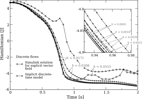
Fig. 3: Results of the numerical experiment. The Hamiltonian function is plotted against time. The explicit model (simulated using Matlab’s module Simulink) is compared with the implicit model (simulated using a Matlab script). As expected, $H$ is monotonically decreasing when $h$ is small enough and the time series converges as $h$ goes to zero.

The sampled-data model was tested using the parameters shown in Table 1. For illustration purposes, we chose a damping control $u_{\alpha}=-0.3\cdot y_{\alpha}$ and simulated the closed-loop system using the sampled-data model (36). Figure 3 shows the discrete-time series of $H$ for different values of $h$. It can be seen that the time series converge and, as expected, the value of $H_{\alpha}$ decreases monotonically when $h$ is small enough (in this case, less or equal to 30 [ m s ]). For comparison purposes, we have included the evolution of $H$ that is obtained by simulating (with Matlab’s Simulink) the explicit model developed in [4] in series with a sampler and a zero-order hold.

5 Conclusions

We have extended the second-order integration method presented in [27]. The original method applies to autonomous Hamiltonian systems and, being symplectic, preserves the Hamiltonian structure of the continuous-time system. The extended method can be applied to port-Hamiltonian systems, which are Hamiltonian systems equipped with input–output pairs. The extended method preserves the port-Hamiltonian structure. Affinity in the controls is lost by the method but, fortunately, the passivity properties of the continuous-time system can be recovered by a suitable redefinition of the output. Interestingly, the relation between the original and the new output is also of second order.

The integration method can be used with the purposes of numerical simulation or with the purpose of deriving discrete-time models to be used in the design of discrete-time control laws.

References

• [1] Vladimir I. Arnold, Mathematical methods of classical mechanics, Springer-Verlag, New York, 1989.
• [2]  , Ordinary Differential Equations, Springer-Verlag, Berlin, 1992.
• [3] Vladimir I. Arnold, Valery Kozlov, and Anatoly I. Neishtadt, Mathematical aspects of classical and celestial mechanics, Springer-Verlag, 2006.
• [4] Fernando Castaños, Dmitry Gromov, Vincent Hayward, and Hannah Michalska, Implicit and explicit representations of continuous-time port-Hamiltonian systems, Systems and Control Lett., 62 (2013), pp. 324 – 330.
• [5] P. J. Channell and F. R. Neri, Symplectic integrators, in Integration Algorithms and Classical Mechanics, Jerrold E. Marsden, George W. Patrick, and William F. Shadwick, eds., AMS, Rhode Island, 1996, pp. 45 – 57.
• [6] Morten Dalsmo and Arjan J. van der Schaft, On representations and integrability of mathematical structures in energy-conserving physical systems, SIAM J. Control Optim., 37 (1999), pp. 54 – 91.
• [7] Zhong Ge and Jerrold E. Marsden, Lie-Poisson Hamilton-Jacobi theory and Lie-Poisson integrators, Physical Review Letters A, 133 (1988), pp. 134 – 139.
• [8] Herbert Goldstein, Charles P. Poole, and John L. Safko, Classical Mechanics, Addison Wesley, 2002.
• [9] Oscar González, Design and analysis of conserving integrators for nonlinear Hamiltonian systems with symmetry, PhD thesis, Stanford University, 1996.
• [10] Oscar González, Mechanical systems subject to holonomic constraints: Differential–algebraic formulations and conservative integration, Physica D, 132 (1999), pp. 165 – 174.
• [11] Ernst Hairer, Christian Lubich, and Gerhard Wanner, Geometric numerical integration: structure-preserving algorithms for ordinary differential equations, Springer-Verlag, 2006.
• [12] Robert A. LaBudde and Donald Greenspan, Energy and momentum conserving methods of arbitrary order for the numerical integration of equations of motion. I. motion of a single particle, Numer. Math., 25 (1976), pp. 323 – 346.
• [13]  , Energy and momentum conserving methods of arbitrary order for the numerical integration of equations of motion. II. motion of a system of particles, Numer. Math., 26 (1976), pp. 1 – 16.
• [14] Dina Shona Laila and Alessandro Astolfi, On the construction of discrete-time model for port-controlled Hamiltonian systems with applications, Systems and Control Lett., 55 (2006), pp. 673 – 680.
• [15]  , Direct discrete-time design for sampled-data Hamiltonian control systems, in Lagrangian and Hamiltonian Methods for Nonlinear Control 2006, Francesco Bullo and Kenji Fujimoto, eds., Springer, 2007, pp. 87 – 98.
• [16] John M. Lee, Introduction to Smooth Manifolds, Springer-Verlag, New York, 2003.
• [17] Benedict Leimkuhler and Sebastian Reich, Simulating Hamiltonian Dynamics, Cambrige University Press, Cambridge, UK, 2004.
• [18] Wei Lin, Feedback stabilization of general nonlinear control systems: A passive system approach, Systems and Control Lett., 25 (1995), pp. 41 – 52.
• [19] Jerrold E. Marsden and Tudor S. Ratiu, Introduction to Mechanics and Symmetry, Springer-Verlag, New York, 1999.
• [20] Bernhard Maschke, Arjan J. van der Schaft, and Peter C. Breedveld, An intrinsic Hamiltonian formulation of network dynamics: Non-standard Poisson structures and gyrators, Journal of the Franklin Institute, 329 (1992), pp. 923 – 966.
• [21] S. Monaco and Dorothée Normand-Cyrot, Advanced tools for nonlinear sampled-data systems’ analysis and control, European Journal of Control, 13 (2007), pp. 221 – 241.
• [22] Peter J. Olver, Applications of Lie groups to differential equations, Springer-Verlag, New York, 1993.
• [23] Romeo Ortega, Arjan J. van der Schaft, Iven Mareels, and Bernhard Maschke, Putting energy back in control, IEEE Control Syst. Mag., (2001), pp. 18–33.
• [24] Romeo Ortega, Arjan J. van der Schaft, Bernhard Maschke, and Gerardo Escobar, Interconnection and damping assignment passivity-based control of port-controlled Hamiltonian systems, Automatica, 38 (2002), pp. 585 – 596.
• [25] Sebastian Reich, On a geometrical interpretation of differential-algebraic equations, Circuits Syst. Signal Process., 9 (1990), pp. 367 – 382.
• [26]  , On an existence and uniqueness theory for nonlinear differential-algebraic equations, Circuits Syst. Signal Process., 10 (1991), pp. 343 – 359.
• [27]  , Symplectic integration of constrained Hamiltonian systems by composition methods, SIAM J. Numer. Anal., 33 (1996), pp. 475 – 491.
• [28] Werner C. Rheinboldt, Differential-algebraic systems as differential equations on manifolds, Mathematics of computation, 43 (1984), pp. 473–482.
• [29]  , On the existence and uniqueness of solutions of nonlinear semi-implicit differential-algebraic equations, Nonlinear Analysis. Theory, Methods and Applications, 16 (1991), pp. 647 – 661.
• [30] J. C. Simo, N. Tarnow, and K. K. Wong, Exact energy-momentum conserving algorithms and symplectic schemes for nonlinear dynamics, Int. J. Numerical Methods in Engineering, 100 (1992), pp. 63 – 116.
• [31] J. C. Simo and K. K. Wong, Unconditionally stable algorithms for rigid body dynamics that exactly preserve energy and momentum, Int. J. Numerical Methods in Engineering, 31 (1991), pp. 19 – 52.
• [32] Arjan J. van der Schaft, $\mathcal{L}_{2}$-Gain and Passivity Techniques in Nonlinear Control, Springer-Verlag, London, 2000.
• [33] Veeravalli S. Varadarajan, Lie Groups, Lie Algebras, and Their Representations, Springer-Verlag, New York, 1984.
• [34] Haruo Yoshida, Construction of higher order symplectic integrators, Physics Letters A, 150 (1990), pp. 262 – 268.