BDgraph: An R Package for Bayesian Structure Learning in Graphical Models

Ernst C. Wit, Second Author BDgraph: An R Package for Bayesian Structure Learning in Graphical Models BDgraph: An R Package for Bayesian Structure Learning in Graphical Models Graphical models provide powerful tools to uncover complicated patterns in multivariate data and are commonly used in Bayesian statistics and machine learning. In this paper, we introduce an R package BDgraph which performs Bayesian structure learning for general undirected graphical models (decomposable and non-decomposable) with continuous, discrete, and mixed variables. The package efficiently implements recent improvements in the Bayesian literature, including that of mohammadi2015bayesianStructure and dobra2018. To speed up computations, the computationally intensive tasks have been implemented in C++ and interfaced with R, and the package has parallel computing capabilities. In addition, the package contains several functions for simulation and visualization, as well as several multivariate datasets taken from the literature and are used to describe the package capabilities. The paper includes a brief overview of the statistical methods which have been implemented in the package. The main body of the paper explains how to use the package. Furthermore, we illustrate the package’s functionality in both real and artificial examples. Bayesian structure learning, Gaussian graphical models, Gaussian copula, Covariance selection, Birth-death process, Markov chain Monte Carlo, G-Wishart, BDgraph, R Bayesian structure learning, Gaussian graphical models, Gaussian copula, Covariance selection, Birth-death process, Markov chain Monte Carlo, G-Wishart, BDgraph, R Reza Mohammadi,
Operation Management Section,
Faculty of Economics end Business,
University of Amsterdam,
Amsterdam, Netherlands,
E-mail:
URL: http://www.uva.nl/profile/a.mohammadi Ernst C. Wit,
Institute of Computational Science,
Universita della Svizzera Italiana,
Lugano, Switzerland,
E-mail:
URL: http://www.math.rug.nl/~ernst/

1 Introduction

Graphical models (lauritzen1996graphical) are commonly used, particularly in Bayesian statistics and machine learning, to describe the conditional independence relationships among variables in multivariate data. In graphical models, each random variable is associated with a node in a graph and links represent conditional dependency between variables, whereas the absence of a link implies that the variables are independent conditional on the rest of the variables (the pairwise Markov property).

In recent years, significant progress has been made in designing efficient algorithms to discover graph structures from multivariate data (dobra2011bayesian; dobra2011copula; jones2005experiments; dobra2018; mohammadi2015bayesianStructure; mohammadi2016bayesian; friedman2008sparse; meinshausen2006high; murray2004bayesian; pensar2017marginal; rolfs2012iterative; wit2015factorial; wit2015inferring; dyrba2018comparison; behrouzi2019detecting). Bayesian approaches provide a principled alternative to various penalized approaches.

In this paper, we describe the BDgraph package (BDgraph) in R (Rcoreteam) for Bayesian structure learning in undirected graphical models. The package can deal with Gaussian, non-Gaussian, discrete and mixed datasets. The package includes various functional modules, including data generation for simulation, several search algorithms, graph estimation routines, a convergence check and a visualization tool; see Figure 1. Our package efficiently implements recent improvements in the Bayesian literature, including those of mohammadi2015bayesianStructure; mohammadi2016bayesian; dobra2018; lenkoski2013direct; mohammadi2017ratio; dobra2011copula; hoff2007extending. For a Bayesian framework of Gaussian graphical models, we implement the method developed by mohammadi2015bayesianStructure and for Gaussian copula graphical models we use the method described by mohammadi2016bayesian and dobra2011copula. To make our Bayesian methods computationally feasible for moderately high-dimensional data, we efficiently implement the BDgraph package in C++ linked to R. To make the package easy to use, the BDgraph package uses several S3 classes as return values of its functions. The package is available under the general public license (GPL $\geq 3$) from the Comprehensive R Archive Network (CRAN) at http://cran.r-project.org/packages=BDgraph.

In the Bayesian literature, the BDgraph is one of the few R packages which is available online for Gaussian graphical models and Gaussian copula graphical models. Another R package is ssgraph (ssgraph) which is based on spike-and-slab proir. On the other hand, more packages seem to be available in the frequentist literature. The existing packages include huge (huge), glasso (glasso), bnlearn (scutari2009learning), pcalg (kalisch2012causal), netgwas (behrouzi2017netgwas), and QUIC (quic; hsieh2014quic).

In Section 2 we illustrate the user interface of the BDgraph package. In Section 3 we explain some methodological background of the package. In this regard, in Section 3.1 we briefly explain the Bayesian framework for Gaussian graphical models for continuous data. In Section 3.2 we briefly describe the Bayesian framework in the Gaussian copula graphical models for data that do not follow the Gaussianity assumption, such as non-Gaussian continuous, discrete or mixed data. In Section 4 we describe the main functions implemented in the BDgraph package. In addition, we explain the user interface and the performance of the package by a simple simulation example. In Section LABEL:sec:real_data, using the functions implemented in the BDgraph package, we study two actual datasets.

2 User interface

In the R environment, one can access and load the BDgraph package by using the following commands: R> install.packages( "BDgraph" ) R> library( "BDgraph" ) By loading the BDgraph package we automatically load the igraph (igraph) package, since the BDgraph package depends on this package for graph visualization. The igraph package is available on the Comprehensive R Archive Network (CRAN) at http://CRAN.R-project.org.

To speed up computations, we efficiently implement the BDgraph package by linking the C++ code to R. The computationally extensive tasks of the package are implemented in parallel in C++ using OpenMP (openmp08). For the C++ code, we use the highly optimized LAPACK (laug) and BLAS (lawson1979basic) linear algebra libraries on systems that provide them. The use of these libraries significantly improves program speed.

We design the BDgraph package to provide a Bayesian framework for undirected graph estimation of different types of datasets such as continuous, discrete or mixed data. The package facilitates a pipeline for analysis by three functional modules; see Figure 1. These modules are as follows:

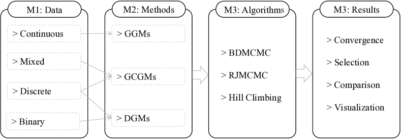
Figure 1: Configuration of the BDgraph package which includes three main parts: (M1) data simulation, (M2) several statistical methods, (M3) several search algorithms, (M4) various functions to evaluate convergence of the search algorithms, estimation of the true graph, assessment and comparison of the results and graph visualization.

Module 1. Data simulation: Function bdgraph.sim simulates multivariate Gaussian, discrete, binary, and mixed data with different undirected graph structures, including "random", "cluster", "scale-free", "lattice", "hub", "star", "circle", "AR(1)", "AR(2)", and "fixed" graphs. Users can determine the sparsity of the graph structure and can generate mixed data, including "count", "ordinal", "binary", "Gaussian" and "non-Gaussian" variables.

Module 2. Methods: The function bdgraph and bdgraph.mpl provide several estimation methods regarding to the type of data:

• Bayesian graph estimation for the multivariate data that follow the Gaussianity assumption, based on the Gaussian graphical models (GGMs); see mohammadi2015bayesianStructure; dobra2011bayesian.

• Bayesian graph estimation for multivariate non-Gaussian, discrete, and mixed data, based on Gaussian copula graphical models (GCGMs); see mohammadi2016bayesian; dobra2011copula.

• Bayesian graph estimation for multivariate discrete and binary data, based on discrete graphical models (DGMs); see dobra2018.

Module 3. Algorithms: The function bdgraph and bdgraph.mpl provide several sampling algorithms:

• Birth-death MCMC (BDMCMC) sampling algorithms (Algorithms 2 and 3) desciribed in mohammadi2015bayesianStructure.

• Reversible jump MCMC (RJMCMC) sampling algorithms desciribed in dobra2011copula.

• Hill-climbing (HC) search algorithm desciribed in pensar2017marginal.

Module 4. Results: Includes four types of functions:

• Graph selection: The functions select, plinks, and pgraph provide the selected graph, the posterior link inclusion probabilities and the posterior probability of each graph, respectively.

• Convergence check: The functions plotcoda and traceplot provide several visualization plots to monitor the convergence of the sampling algorithms.

• Comparison and goodness-of-fit: The functions compare and plotroc provide several comparison measures and an ROC plot for model comparison.

• Visualization: The plotting functions plot.bdgraph and plot.sim provide visualizations of the simulated data and estimated graphs.

3 Methodological background

In Section 3.1, we briefly explain the Gaussian graphical model for multivariate data. Then we illustrate the birth-death MCMC algorithm for sampling from the joint posterior distribution over Gaussian graphical models; for more details see mohammadi2015bayesianStructure. In Section 3.2, we briefly describe the Gaussian copula graphical model (dobra2011copula), which can deal with non-Gaussian, discrete or mixed data. Then we explain the birth-death MCMC algorithm which is designed for the Gaussian copula graphical models; for more details see mohammadi2016bayesian.

3.1 Bayesian Gaussian graphical models

In graphical models, each random variable is associated with a node and conditional dependence relationships among random variables are presented as a graph $G=(V,E)$ in which $V=\{1,2,...,p\}$ specifies a set of nodes and a set of existing links $E\subset V\times V$ (lauritzen1996graphical). Our focus here is on undirected graphs, in which $(i,j)\in E\Leftrightarrow(j,i)\in E$. The absence of a link between two nodes specifies the pairwise conditional independence of those two variables given the remaining variables, while a link between two variables determines their conditional dependence.

In Gaussian graphical models (GGMs), we assume that the observed data follow multivariate Gaussian distribution $\mathcal{N}_{p}(\mu,K^{-1})$. Here we assume $\mu=0$. Let $\mathbf{Z}=(Z^{(1)},...,Z^{(n)})^{\top}$ be the observed data of $n$ independent samples, then the likelihood function is

$$Pr(\mathbf{Z}|K,G)\propto|K|^{n/2}\exp\left\{-\frac{1}{2}\mbox{tr}(KU)\right\},$$ (1)

where $U=\mathbf{Z}^{\top}\mathbf{Z}$.

In GGMs, conditional independence is implied by the form of the precision matrix. Based on the pairwise Markov property, variables $i$ and $j$ are conditionally independent given the remaining variables, if and only if $K_{ij}=0$. This property implies that the links in graph $G=(V,E)$ correspond with the nonzero elements of the precision matrix $K$; this means that $E=\{(i,j)|K_{ij}\neq 0\}$. Given graph $G$, the precision matrix $K$ is constrained to the cone $\mathbb{P}_{G}$ of symmetric positive definite matrices with elements $K_{ij}$ equal to zero for all $(i,j)\notin E$.

We consider the G-Wishart distribution $W_{G}(b,D)$ to be a prior distribution for the precision matrix $K$ with density

$$Pr(K|G)=\frac{1}{I_{G}(b,D)}|K|^{(b-2)/2}\exp\left\{-\frac{1}{2}\mbox{tr}(DK)\right\}1(K\in\mathbb{P}_{G}),$$ (2)

where $b>2$ is the degrees of freedom, $D$ is a symmetric positive definite matrix, $I_{G}(b,D)$ is the normalizing constant with respect to the graph $G$ and $1(x)$ evaluates to $1$ if $x$ holds, and otherwise to $0$. The G-Wishart distribution is a well-known prior for the precision matrix, since it represents the conjugate prior for multivariate Gaussian data as in (1).

For full graphs, the G-Wishart distribution reduces to the standard Wishart distribution, hence the normalizing constant has an explicit form (muirhead1982aspects). Also, for decomposable graphs, the normalizing constant has an explicit form (roverato2002hyper); however, for non-decomposable graphs, it does not. In that case it can be estimated by using the Monte Carlo method (atay2005monte), the Laplace approximation (lenkoski2011computational), or recent approximation by mohammadi2017ratio. In the BDgraph package, we design the gnorm function to estimate the log of the normalizing constant by using the Monte Carlo method proposed atay2005monte.

Since the G-Wishart prior is a conjugate prior to the likelihood (1), the posterior distribution of $K$ is

$$Pr(K|\mathbf{Z},G)=\frac{1}{I_{G}(b^{*},D^{*})}|K|^{(b^{*}-2)/2}\exp\left\{-\frac{1}{2}\mbox{tr}(D^{*}K)\right\},$$

where $b^{*}=b+n$ and $D^{*}=D+S$, that is, $W_{G}(b^{*},D^{*})$.

3.1.1 Direct sampler from G-Wishart

Several sampling methods from the G-Wishart distribution have been proposed; to review existing methods see wang2012efficient. More recently, lenkoski2013direct has developed an exact sampling algorithm for the G-Wishart distribution, borrowing an idea from hastie2009elements.

Algorithm 1 . Exact sampling from the precision matrix

0:  A graph $G=(V,E)$ with precision matrix $K$ and $\Sigma=K^{-1}$

0:  An exact sample from the precision matrix.

1:  Set $\Omega=\Sigma$

2:  repeat

3:     for $i=1,...,p$ do

4:        Let $N_{i}\subset V$ be the neighbor set of node $i$ in $G$. Form $\Omega_{N_{i}}$ and $\Sigma_{N_{i},i}$ and solve $\hat{\beta_{i}^{*}}=\Omega^{-1}_{N_{i}}\Sigma_{N_{i},i}$

5:        Form $\hat{\beta_{i}}\in R^{p-1}$ by padding the elements of $\hat{\beta_{i}^{*}}$ to the appropriate locations and zeros in those locations not connected to $i$ in $G$

6:        Update $\Omega_{i,-i}$ and $\Omega_{-i,i}$ with $\Omega_{-i,-i}\hat{\beta_{i}}$

7:     end for

8:  until  convergence

9:  return  $K=\Omega^{-1}$

In the BDgraph package, we use Algorithm 1 to sample from the posterior distribution of the precision matrix. We implement the algorithm in the package as a function rgwish; see the R code below for illustration. R> adj <- matrix( c( 0, 0, 1, 0, 0, 0, 1, 0, 0 ), 3, 3 ) R> adj [,1] [,2] [,3] [1,] 0 0 1 [2,] 0 0 0 [3,] 1 0 0 R> sample <- rgwish( n = 1, adj = adj, b = 3, D = diag( 3 ) ) R> round( sample, 2 ) [,1] [,2] [,3] [1,] 2.37 0.00 -2.12 [2,] 0.00 6.15 0.00 [3,] -2.12 0.00 7.26 This matrix is a sample from a G-Wishart distribution with $b=3$ and $D=I_{3}$ as an identity matrix and a graph structure with adjacency matrix adj.

3.1.2 BDMCMC algorithm for GGMs

Consider the joint posterior distribution of the graph $G$ and the precision matrix $K$ given by

$$Pr(K,G\mid\mathbf{Z})\propto Pr(\mathbf{Z}\mid K)~{}Pr(K\mid G)~{}Pr(G).$$ (3)

For the prior distribution of the graph $G=(V,E)$, we consider a Bernoulli prior on each link inclusion indicator variable as follow

$$Pr(G)\propto\left(\frac{\theta}{1-\theta}\right)^{|E|},$$ (4)

where $|E|$ indicate the number of links in the graph $G$ (graph size) and parameter $\theta\in(0,1)$ is a prior probability of existing link. For the case $\theta=0.5$ (as a default option of the BDgraph), we will have a uniform distribution over all graph space, as a non-informative prior. For the prior distribution of the precision matrix conditional on the graph $G$, we use a G-Wishart $W_{G}(b,D)$.

Here we consider a computationally efficient birth-death MCMC sampling algorithm proposed by mohammadi2015bayesianStructure for Gaussian graphical models. The algorithm is based on a continuous time birth-death Markov process, in which the algorithm explores the graph space by adding/removing a link in a birth/death event.

In the birth-death process, for a particular pair of graph $G=(V,E)$ and precision matrix $K$, each link dies independently of the rest as a Poisson process with death rate $\delta_{e}(K)$. Since the links are independent, the overall death rate is $\delta(K)=\sum_{e\in E}\delta_{e}(K)$. Birth rates $\beta_{e}(K)$ for $e\notin E$ are defined similarly. Thus the overall birth rate is $\beta(K)=\sum_{e\notin E}\beta_{e}(K)$.

Since the birth and death events are independent Poisson processes, the time between two successive events is exponentially distributed with mean $1/(\beta(K)+\delta(K))$. The time between successive events can be considered as inverse support for any particular instance of the state $(G,K)$. The probabilities of birth and death events are

$$Pr(\mbox{birth of link }e)=\frac{\beta_{e}(K)}{\beta(K)+\delta(K)},\qquad\mbox{for each}\ \ e\notin E,$$ (5)

$$Pr(\mbox{death of link }e)=\frac{\delta_{e}(K)}{\beta(K)+\delta(K)},\qquad\mbox{for each}\ \ e\in E.$$ (6)

The birth and death rates of links occur in continuous time with the rates determined by the stationary distribution of the process. The BDMCMC algorithm is designed in such a way that the stationary distribution is equal to the target joint posterior distribution of the graph and the precision matrix (3).

mohammadi2015bayesianStructure derived a condition that guarantees the above birth and death process converges to our target joint posterior distribution (3). By following their Theorem we define the birth and death rates, as below

$$\beta_{e}(K)=\min\left\{\frac{Pr(G^{+e},K^{+e}|\mathbf{Z})}{Pr(G,K|\mathbf{Z})},1\right\},\ \ \mbox{for each}\ \ e\notin E,$$ (7)

$$\delta_{e}(K)=\min\left\{\frac{Pr(G^{-e},K^{-e}|\mathbf{Z})}{Pr(G,K|\mathbf{Z})},1\right\},\ \ \mbox{for each}\ \ e\in E,$$ (8)

in which $G^{+e}=(V,E\cup\{e\})$ and $K^{+e}\in\mathbb{P}_{G^{+e}}$ and similarly $G^{-e}=(V,E\setminus\{e\})$ and $K^{-e}\in\mathbb{P}_{G^{-e}}$. For computation part related to the ratio of posterior see mohammadi2017ratio.

Algorithm 2 provides the pseudo-code for our BDMCMC sampling scheme which is based on the above birth and death rates.

Algorithm 2 . BDMCMC algorithm for GGMs

0:  A graph $G=(V,E)$ and a precision matrix $K$.

0:  Samples from the joint posterior distribution of $(G,K)$, (3), and waiting times.

1:  for N iteration do

2:     1. Sample from the graph. Based on birth and death process

3:         1.1. Calculate the birth rates by (7) and $\beta(K)=\sum_{e\in\notin E}{\beta_{e}(K)}$

4:         1.2. Calculate the death rates by (8) and $\delta(K)=\sum_{e\in E}{\delta_{e}(K)}$

5:         1.3. Calculate the waiting time by $W(K)=1/(\beta(K)+\delta(K))$

6:         1.4. Simulate the type of jump (birth or death) by (5) and (6)

7:     2. Sample from the precision matrix. By using Algorithm 1.

8:  end for

Note, step $1$ of the algorithm is suitable for parallel computation. In the BDgraph, we implement this step of algorithm in parallel using OpenMP in C++ to speed up the computations.

The BDMCMC sampling algorithm is designed in such a way that a sample $(G,K)$ is obtained at certain jump moments, $\{t_{1},t_{2},...\}$ (see Figure 2). For efficient posterior inference of the parameters, we use the Rao-Blackwellized estimator, which is an efficient estimator for continuous time MCMC algorithms (cappe2003reversible, Section 2.5). By using the Rao-Blackwellized estimator, for example, one can estimate the posterior distribution of the graphs proportional to the total waiting times of each graph.

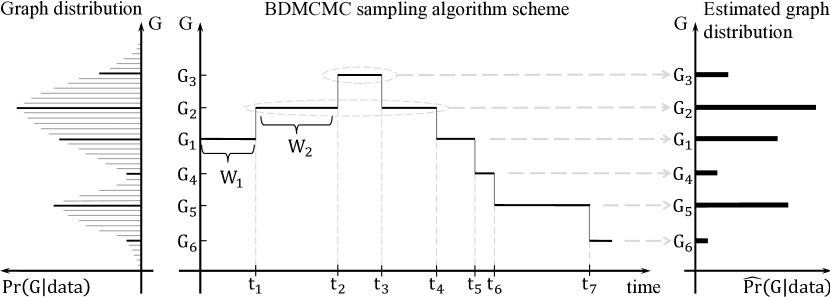
Figure 2: This image visualizes the Algorithm 2. The left side shows the true posterior distribution of the graph. The middle panel presents a continuous time BDMCMC sampling algorithm where $\left\{W_{1},W_{2},...\right\}$ denote waiting times and $\left\{t_{1},t_{2},...\right\}$ denote jumping times. The right side denotes the estimated posterior probability of the graphs in proportion to the total of their waiting times, according to the Rao-Blackwellized estimator.

3.2 Gaussian copula graphical models

In practice we encounter both discrete and continuous variables; Gaussian copula graphical modelling has been proposed by dobra2011copula to describe dependencies between such heterogeneous variables. Let $\mathbf{Y}$ (as observed data) be a collection of continuous, binary, ordinal or count variables with the marginal distribution $F_{j}$ of $Y_{j}$ and $F_{j}^{-1}$ as its pseudo inverse. For constructing a joint distribution of $\mathbf{Y}$, we introduce a multivariate Gaussian latent variable as follows:

$$Z_{1},...,Z_{n}\stackrel{{\scriptstyle iid}}{{\sim}}\mathcal{N}_{p}(0,\Gamma(K)),$$

$$Y_{ij}=F_{j}^{-1}(\Phi(Z_{ij})),$$ (9)

where $\Gamma(K)$ is the correlation matrix for a given precision matrix $K$. The joint distribution of $\mathbf{Y}$ is given by

$$Pr\left(Y_{1}\leq Y_{1},\ldots,Y_{p}\leq Y_{p}\right)=C(F_{1}(Y_{1}),\ldots,F_{p}(Y_{p})\mid\Gamma(K)),$$ (10)

where $C(\cdot)$ is the Gaussian copula given by

$$C(u_{1},\ldots,u_{p}\mid\Gamma)=\Phi_{p}\left(\Phi^{-1}(u_{1}),\ldots,\Phi^{-1}(u_{p})\mid\Gamma\right),$$

with $u_{v}=F_{v}(Y_{v})$ and $\Phi_{p}(\cdot)$ is the cumulative distribution of multivariate Gaussian and $\Phi(\cdot)$ is the cumulative distribution of univariate Gaussian distributions. It follows that $Y_{v}=F_{v}^{-1}\left(\Phi(Z_{v})\right)$ for $v={1,...,p}$. If all variables are continuous then the margins are unique; thus zeros in $K$ imply conditional independence, as in Gaussian graphical models (hoff2007extending; abegaz2015copula). For discrete variables, the margins are not unique but still well-defined (nelsen2007introduction).

In semiparametric copula estimation, the marginals are treated as nuisance parameters and estimated by the rescaled empirical distribution. The joint distribution in (10) is then parametrized only by the correlation matrix of the Gaussian copula. We are interested to infer the underlying graph structure of the observed variables $\mathbf{Y}$ implied by the continuous latent variables $\mathbf{Z}$. Since $\mathbf{Z}$ are unobservable we follow the idea of hoff2007extending of associating them with the observed data as below.

Given the observed data $\mathbf{Y}$ from a sample of $n$ observations, we constrain the samples from latent variables $\mathbf{Z}$ to belong to the set

$$\mathcal{D}(\mathbf{Y})=\{\mathbf{Z}\in\mathbb{R}^{n\times p}:L_{j}^{r}(\mathbf{Z})<z_{j}^{(r)}<U_{j}^{r}(\mathbf{Z}),r=1,\ldots,n;j=1,\ldots,p\},$$

where

$$L_{j}^{r}(\mathbf{Z})=\max\left\{Z_{j}^{(s)}:Y_{j}^{(s)}<Y_{j}^{(r)}\right\}\mbox{ and }U_{j}^{r}(\mathbf{Z})=\min\left\{Z_{j}^{(s)}:Y_{j}^{(r)}<Y_{j}^{(s)}\right\}.$$ (11)

Following hoff2007extending we infer the latent space by substituting the observed data $\mathbf{Y}$ with the event $\mathcal{D}(\mathbf{Y})$ and define the likelihood as

$$Pr(\mathbf{Y}\mid K,G,F_{1},...,F_{p})=Pr(\mathbf{Z}\in\mathcal{D}(\mathbf{Y})\mid K,G)~{}Pr(\mathbf{Y}\mid\mathbf{Z}\in\mathcal{D}(\mathbf{Y}),K,G,F_{1},...,F_{p}).$$

The only part of the observed data likelihood relevant for inference on $K$ is $Pr(\mathbf{Z}\in\mathcal{D}(\mathbf{Y})\mid K,G)$. Thus, the likelihood function is given by

$$Pr(\mathbf{Z}\in\mathcal{D}(\mathbf{Y})\mid K,G)=Pr(\mathbf{Z}\in\mathcal{D}(\mathbf{Y})\mid K,G)=\int_{\mathcal{D}(\mathbf{Y})}Pr(\mathbf{Z}\mid K,G)dZ$$ (12)

where $Pr(\mathbf{Z}\mid K,G)$ is defined in (1).

3.2.1 BDMCMC algorithm for GCGMs

The joint posterior distribution of the graph $G$ and precision matrix $K$ for the GCGMs is

$$Pr(K,G|Z\in\mathcal{D}(\mathbf{Y}))\propto Pr(K,G)Pr(Z\in\mathcal{D}(\mathbf{Y})|K,G).$$ (13)

Sampling from this posterior distribution can be done by using the birth-death MCMC algorithm. mohammadi2016bayesian have developed and extended the birth-death MCMC algorithm to more general cases of GCGMs. We summarize their algorithm as follows:

Algorithm 3 . BDMCMC algorithm for GCGMs

0:  A graph $G=(V,E)$ and a precision matrix $K$.

0:  Samples from the joint posterior distribution of $(G,K)$, (13), and waiting times.

1:  for N iteration do

2:     1. Sample the latent data. For each $r\in V$ and $j\in\{1,...,n\}$, we update the latent values from its full conditional distribution as follows

$$Z_{r}^{(j)}|Z_{V\setminus\{r\}}=z_{V\setminus\{r\}}^{(j)},K\sim N(-\sum_{r^{\prime}}{K_{rr^{\prime}}z_{r^{\prime}}^{(j)}/K_{rr}},1/K_{rr}),$$

truncated to the interval $\left[L_{r}^{j}(\mathbf{Z}),U_{r}^{j}(\mathbf{Z})\right]$ in (11).

3:     2. Sample from the graph. Same as step $1$ in Algorithm 2.

4:     3. Sample from the precision matrix. By using Algorithm 1.

5:  end for

In step $1$, the latent variables $\mathbf{Z}$ are sampled conditional on the observed data $\mathbf{Y}$. The other steps are the same as in Algorithm 2.

Remark: in cases where all variables are continuous, we do not need to sample from latent variables in each iteration of Algorithm 2, since all margins in the Gaussian copula are unique. Thus, for these cases, we transfer our non-Gaussian data to Gaussian, and then we run Algorithm 2; see example LABEL:subsec:gene_data.

3.2.2 Alternative RJMCMC algorithm

RJMCMC is a special case of the trans-dimensional MCMC methodology green2003trans. The RJMCMC approach is based on an ergodic discrete-time Markov chain. In graphical models, a RJMCMC algorithm can be designed in such a way that its stationary distribution is the joint posterior distribution of the graph and the parameters of the graph, e.g., 3 for GGMs and 13 for GCGMs.

A RJMCMC can be implemented in various different ways. giudici1999decomposable implemented this algorithm only for the decomposable GGMs, because of the expensive computation of the normalizing constant $I_{G}(b,D)$. The RJMCMC approach developed by dobra2011bayesian and dobra2011copula is based on the Cholesky decomposition of the precision matrix. It uses an approximation for dealing with the extensive computation of the normalizing constant. To avoid the intractable normalizing constant calculation, lenkoski2013direct and wang2012efficient implemented a special case of RJMCMC algorithm, which is based on the exchange algorithm (murray2012mcmc). Our implementation of RJMCMC algorithm in the BDgraph package defines the acceptance probability proportional to the birth/death rates in our BDMCMC algorithm. Moreover, we implement the exact sampling of G-Wishart distribution, as described in Section 3.1.1. Besides, we using the result of mohammadi2017ratio for the ratio of the normalizing constant of G-Wishart distribution.

4 The BDgraph environment

The BDgraph package provides a set of comprehensive tools related to Bayesian graphical models; we describe below the essential functions available in the package.

4.1 Posterior sampling

We design the function bdgraph, as the main function of the package, to take samples from the posterior distributions based on both of our Bayesian frameworks (GGMs and GCGMs). By default, the bdgraph function is based on underlying sampling algorithms (Algorithms 2 and 3). Moreover, as an alternative to those BDMCMC sampling algorithms, we implement RJMCMC sampling algorithms for both the Gaussian and non-Gaussian frameworks. By using the following function bdgraph( data, n = NULL, method = "ggm", algorithm = "bdmcmc", iter = 5000, burnin = iter / 2, not.cont = NULL, g.prior = 0.5, df.prior = 3, g.start = "empty", jump = NULL, save = FALSE, print = 1000, cores = NULL, threshold = 1e-8 ) we obtain a sample from our target joint posterior distribution. bdgraph returns an object of S3 class type “bdgraph”. The functions plot, print and summary are working with the object “bdgraph”. The input data can be an ($n\times p$) matrix or a data.frame or a covariance ($p\times p$) matrix ($n$ is the sample size and $p$ is the dimension); it can also be an object of class “sim”, which is the output of function bdgraph.sim.

The argument method determines the type of methods, GGMs, GCGMs. Option “ggm” is based on Gaussian graphical models (Algorithm 2) that is designed for multivariate Gaussian data. Option “gcgm” is based on the GCGMs (Algorithm 3) that is designed for non-Gaussian data such as, non-Gaussian continuous, discrete or mixed data.

The argument algorithm refers the type of sampling algorithms which could be based on BDMCMC or RJMCMC. Option “bdmcmc” (as default) is for the BDMCMC sampling algorithms (Algorithms 2 and 3). Option “rjmcmc” is for the RJMCMC sampling algorithms, which are alternative algorithms. See mohammadi2015bayesianStructure, mohammadi2016bayesian.

The argument g.start specifies the initial graph for our sampling algorithm. It could be empty (default) or full. Option empty means the initial graph is an empty graph and full means a full graph. It also could be an object with S3 class "bdgraph", which allows users to run the sampling algorithm from the last objects of the previous run.

The argument jump determines the number of links that are simultaneously updated in the BDMCMC algorithm.

For parallel computation in C++ which is based on OpenMP (openmp08), user can use argument cores which specifies the number of cores to use for parallel execution.

Note, the package BDgraph has two other sampling functions, bdgraph.mpl and bdgraph.ts which are designed in the similar framework as the function bdgraph. The function bdgraph.mpl is for Bayesian model determination in undirected graphical models based on marginal pseudo-likelihood, for both continuous and discrete variables; For more details see dobra2018. The function bdgraph.ts is for Bayesian model determination in time series graphical models (tank2015bayesian).

4.2 Posterior graph selection

We design the BDgraph package in such a way that posterior graph selection can be done based on both Bayesian model averaging (BMA), as default, and maximum a posterior probability (MAP). The functions select and plinks are designed for the objects of class bdgraph to provide BMA and MAP estimations for posterior graph selection.

The function plinks( bdgraph.obj, round = 2, burnin = NULL ) provides estimated posterior link inclusion probabilities for all possible links, which is based on BMA estimation. In cases where the sampling algorithm is based on BDMCMC, these probabilities for all possible links $e=(i,j)$ in the graph can be estimated using a Rao-Blackwellized estimate (cappe2003reversible, Section 2.5) based on

$$Pr(e\in E|data)=\frac{\sum_{t=1}^{N}{1(e\in E^{(t)})W(K^{(t)})}}{\sum_{t=1}^{N}{W(K^{(t)})}},$$ (14)

where $N$ is the number of iteration and $W(K^{(t)})$ are the weights of the graph $G^{(t)}$ with the precision matrix $K^{(t)}$.

The function select( bdgraph.obj, cut = NULL, vis = FALSE ) provides the inferred graph based on both BMA (as default) and MAP estimators. The inferred graph based on BMA estimation is a graph with links for which the estimated posterior probabilities are greater than a certain cut-point (as default cut=0.5). The inferred graph based on MAP estimation is a graph with the highest posterior probability.

Note, for posterior graph selection based on MAP estimation we should save all adjacency matrices by using the option save = TRUE in the function bdgraph. Saving all the adjacency matrices could, however, cause memory problems; to see how we cope with this problem the reader is referred to Appendix LABEL:appendix.

4.3 Convergence check

In general, convergence in MCMC approaches can be difficult to evaluate. From a theoretical point of view, the sampling distribution will converge to the target joint posterior distribution as the number of iteration increases to infinity. Because we normally have little theoretical insight about how quickly MCMC algorithms converge to the target stationary distribution we therefore rely on post hoc testing of the sampled output. In general, the sample is divided into two parts: a “burn-in” part of the sample and the remainder, in which the chain is considered to have converged sufficiently close to the target posterior distribution. Two questions then arise: How many samples are sufficient? How long should the burn-in period be?

The plotcoda and traceplot are two visualization functions for the objects of class bdgraph that make it possible to check the convergence of the search algorithms in BDgraph. The function plotcoda( bdgraph.obj, thin = NULL, control = TRUE, main = NULL, … ) provides the trace of estimated posterior probability of all possible links to check convergence of the search algorithms. Option control is designed for the case where if control=TRUE (as default) and the dimension ($p$) is greater than $15$, then $100$ links are randomly selected for visualization.

The function traceplot( bdgraph.obj, acf = FALSE, pacf = FALSE, main = NULL, … ) provides the trace of graph size to check convergence of the search algorithms. Option acf is for visualization of the autocorrelation functions for graph size; option pacf visualizes the partial autocorrelations.

4.4 Comparison and goodness-of-fit

The functions compare and plotroc are designed to evaluate and compare the performance of the selected graph. These functions are particularly useful for simulation studies. With the function compare( target, est, est2 = NULL, est3 = NULL, est4 = NULL, main = NULL, vis = FALSE ) we can evaluate the performance of the Bayesian methods available in our BDgraph package and compare them with alternative approaches. This function provides several measures such as the balanced $F$-score measure (baldi2000assessing), which is defined as follows:

$$F_{1}\mbox{-score}=\frac{2\mbox{TP}}{2\mbox{TP + FP + FN}},$$ (15)

where TP, FP and FN are the number of true positives, false positives and false negatives, respectively. The $F_{1}$-score lies between $0$ and $1$, where $1$ stands for perfect identification and $0$ for no true positives.

The function plotroc( target, est, est2 = NULL, est3 = NULL, est4 = NULL, cut = 20, smooth = FALSE, label = TRUE, main = "ROC Curve" ) provides a ROC plot for visualization comparison based on the estimated posterior link inclusion probabilities.

4.5 Data simulation

The function bdgraph.sim is designed to simulate different types of datasets with various graph structures. The function bdgraph.sim( p = 10, graph = "random", n = 0, type = "Gaussian", prob = 0.2, size = NULL, mean = 0, class = NULL, cut = 4, b = 3, D = diag( p ), K = NULL, sigma = NULL, vis = FALSE ) can simulate multivariate Gaussian, non-Gaussian, discrete, binary and mixed data with different undirected graph structures, including "random", "cluster", "scale-free", "lattice", "hub", "star", "circle", "AR(1)", "AR(2)", and "fixed" graphs. Users can specify the type of multivariate data by option type and the graph structure by option graph. They can determine the sparsity level of the obtained graph by using option prob. With this function users can generate mixed data from "count", "ordinal", "binary", "Gaussian" and "non-Gaussian" distributions. bdgraph.sim returns an object of the S3 class type “sim”. Functions plot and print work with this object type.

There is another function in the BDgraph package with the name graph.sim which is designed to simulate different types of graph structures. The function graph.sim( p = 10, graph = "random", prob = 0.2, size = NULL, class = NULL, cut = 4, vis = FALSE ) can simulate different undirected graph structures, including "random", "cluster", "scale-free"’, "lattice", "hub", "star", and "circle" graphs. Users can specify the type of graph structure by option graph. They can determine the sparsity level of the obtained graph by using option prob. bdgraph.sim returns an object of the S3 class type “graph”. Functions plot and print work with this object type.

5 An example on simulated data

We illustrate the user interface of the BDgraph package by use of a simple simulation. We perform all the computations on an MacBook Pro with $2.9$ GHz Intel Core i$7$ processor. By using the function bdgraph.sim we simulate $60$ observations ($n=60$) from a multivariate Gaussian distribution with $8$ variables ($p=8$) and “scale-free” graph structure, as below. R> data.sim <- bdgraph.sim( n = 60, p = 8, graph = "scale-free", + type = "Gaussian" ) R> round( head( data.sim $data,4),2)\CodeOutput[,1][,2][,3][,4][,5][,6][,7][,8][1,]0.72-0.91-1.23-0.160.20-0.470.081.07[2,]0.25-0.110.090.530.10-0.04-0.13-0.67[3,]-0.42-0.09-0.28-0.422.040.84-0.791.24[4,]-0.33-0.500.68-1.33-1.150.25-0.352.97\par SincethegenerateddataareGaussian,weruntheBDMCMCalgorithmwhichisbasedonGaussiangraphicalmodels.Forthiswechoose\code{method="ggm"},asfollows:\Sinput R>sample.bdmcmc<-bdgraph(bdgraph(data=data.sim,method="ggm",+algorithm="bdmcmc",iter=5000,save=TRUE)Wechooseoption``\code{save=TRUE}^{\prime\prime}tosavethesamplesinordertocheckconvergenceofthealgorithm.Runningthisfunctiontakeslessthanonesecond,asthecomputationalintensivetasksareperformedin\proglang{C++}andinterfacedwith\proglang{R}.\par Sincethefunction\code{bdgraph}returnsanobjectofclass\code{S3},userscanseethesummaryresultasfollows\Sinput R>summary(sample.bdmcmc)\CodeOutput$selected_{g}[,1][,2][,3][,4][,5][,6][,7][,8][1,]01100010[2,]00010000[3,]00000100[4,]00000001[5,]00000000[6,]00000000[7,]00000000[8,]00000000\par$p_{l}inks[,1][,2][,3][,4][,5][,6][,7][,8][1,]00.511.000.270.210.310.740.11[2,]00.000.291.000.250.180.490.14[3,]00.000.000.240.270.790.440.22[4,]00.000.000.000.320.300.341.00[5,]00.000.000.000.000.250.400.22[6,]00.000.000.000.000.000.230.37[7,]00.000.000.000.000.000.000.19[8,]00.000.000.000.000.000.000.00\par$K_{h}at[,1][,2][,3][,4][,5][,6][,7][,8][1,]3.810.333.19-0.090.040.14-0.840.02[2,]0.334.24-0.06-3.43-0.07-0.020.41-0.02[3,]3.19-0.065.54-0.08-0.06-0.750.410.08[4,]-0.09-3.43-0.089.28-0.150.10-0.181.62[5,]0.04-0.07-0.06-0.150.76-0.060.16-0.04[6,]0.14-0.02-0.750.10-0.063.080.04-0.14[7,]-0.840.410.41-0.180.160.045.560.04[8,]0.02-0.020.081.62-0.04-0.140.041.21\par Thesummaryresultsaretheadjacencymatrixoftheselectedgraph(\code{selected_{g}})basedonBMAestimation,theestimatedposteriorprobabilitiesofallpossiblelinks(\code{p_{l}inks})andtheestimatedprecisionmatrix(\code{K_{h}at}).\par Inaddition,thefunction\code{summary}reportsavisualizationsummaryoftheresultsaswecanseeinFigure\ref{fig:summary-bdgraph}.Atthetop-leftisthegraphwiththehighestposteriorprobability.Theplotatthetop-rightgivestheestimatedposteriorprobabilitiesofallthegraphswhicharevisitedbytheBDMCMCalgorithm;itindicatesthatouralgorithmvisitsmorethan$2000$differentgraphs.Theplotatthebottom-leftgivestheestimatedposteriorprobabilitiesofthesizeofthegraphs;itindicatesthatouralgorithmvisitedmainlygraphswithsizesbetween$4$and$18$links.Atthebottom-rightisthetraceofouralgorithmbasedonthesizeofthegraphs.\text{Figure 3Figure 3Fig.FigureFigs.Figures3Figure 33Visualizationsummaryofsimulationdatabasedonoutputofcodebdgraphfunction.Thefigureatt}$