TRANSPORT BY MERIDIONAL CIRCULATIONS IN SOLAR-TYPE STARS

Abstract

Transport by meridional flows has significant consequences for stellar evolution, but is difficult to capture in global-scale numerical simulations because of the wide range of timescales involved. Stellar evolution models therefore usually adopt parameterizations for such transport based on idealized laminar or mean-field models. Unfortunately, recent attempts to model this transport in global simulations have produced results that are not consistent with any of these idealized models. In an effort to explain the discrepancies between global simulations and idealized models, we here use three-dimensional local Cartesian simulations of compressible convection to study the efficiency of transport by meridional flows below a convection zone in several parameter regimes of relevance to the Sun and solar-type stars. In these local simulations we are able to establish the correct ordering of dynamical timescales, although the separation of the timescales remains unrealistic. We find that, even though the generation of internal waves by convective overshoot produces a high degree of time dependence in the meridional flow field, the mean flow has the qualitative behavior predicted by laminar, “balanced” models. In particular, we observe a progressive deepening, or “burrowing”, of the mean circulation if the local Eddington–Sweet timescale is shorter than the viscous diffusion timescale. Such burrowing is a robust prediction of laminar models in this parameter regime, but has never been observed in any previous numerical simulation. We argue that previous simulations therefore underestimate the transport by meridional flows.

1. INTRODUCTION

1.1. The Role of Meridional Circulations in Transport and Mixing

The interiors of stars, in common with all rotating fluids, frequently exhibit meridional circulations, and the transport of angular momentum and chemical species by these circulations has significant consequences for stellar evolution (e.g., Mestel, 1953; Chaboyer & Zahn, 1992; Pinsonneault, 1997). Within convective zones, transport by meridional circulations is generally less important than transport by turbulent convective motions, but within radiative zones transport by meridional circulations may be a dominant mechanism. Such transport may play a significant role in the spin-down of the Sun’s core (Howard et al., 1967; Spiegel, 1972; Clark, 1975) and the depletion of lithium in solar-type stars (e.g., Charbonneau & Michaud, 1988; Garaud & Bodenheimer, 2010). Meridional flows also transport magnetic flux, a fact that forms the basis of certain theories of the solar magnetic cycle (e.g., Dikpati & Charbonneau, 1999) and the solar interior rotation (Gough & McIntyre, 1998).

In one-dimensional (1D) models of stellar interiors, transport by meridional circulations is sometimes parameterized in terms of a “rotationally-induced mixing” parameter (Zahn, 1992) derived from idealized laminar or mean-field models. Many such models have been proposed, leading to many different prescriptions for transport and mixing, all of which assume that the amplitude and radial extent of the circulation, and hence the degree of mixing, depend only on the spherically-averaged angular velocity, $\Omega(r)$. Such a description is clearly limited: in the Sun, for example, the spherically-averaged angular velocity is almost uniform (Couvidat et al., 2003), yet the latitudinal differential rotation drives a meridional circulation, as described in Section 1.2. Moreover, the validity of such parameterizations has never been confirmed by any 3D numerical model.

In this paper we use a fully compressible, 3D numerical model to study the behavior of meridional flows driven by differential rotation of the convective envelopes of solar-type stars. We compare the results of our simulations with the predictions of both laminar and mean-field models and test the assumptions on which those models are based. In the present work we consider only non-magnetic processes; the effects of magnetic fields will be addressed in future papers. Ultimately, our aim is to construct a better parameterization for the role of meridional flows in transporting angular momentum, chemical species, and magnetic fields in stellar interiors.

The rest of the paper is structured as follows. In Sections 1.2–1.3 we briefly review the physical mechanisms that give rise to meridional flows and discuss their expected behavior in the context of stellar interiors. In Section 1.4 we summarize the results of recent global numerical simulations of angular momentum transport in the solar interior. Our numerical model is described in Section 2, and parameter constraints are outlined in Section 3. In Section 4 we present results from four simulations performed in different parameter regimes. Our findings are summarized in Section 5 and discussed in relation to the results of other studies.

1.2. Driving of Meridional Circulations

The presence of meridional circulations in stellar interiors can be explained by two complementary arguments. The first is a generalization of the classical Vogt–Eddington argument (Vogt, 1925; Eddington, 1925). In a rotating star, a balance between centrifugal, Coriolis, pressure, and gravitational forces in the meridional plane generally requires that temperature is non-constant within each horizontal surface, implying that the radiative heat flux has nonzero divergence. Within a radiative (i.e., non-convecting) zone, advection of entropy by a meridional flow is the only mechanism that can balance the divergence of the heat flux. A meridional circulation must therefore be present in order to maintain local thermal equilibrium and circumvent the so-called “von Zeipel paradox” (e.g., Mestel, 1999, §5.4).

For a given internal rotation profile, we can in principal deduce the meridional flow required to maintain the balances just described. Although it is tempting to say that the rotation profile “drives” the meridional flow, is it more correct to say that the persistence of the rotation profile, on timescales for which meridional force balance and local thermal equilibrium are expected to apply, implies the presence of a meridional flow. The transport of angular momentum by this meridional flow will feed back onto the rotation profile, causing it to evolve over time. The classical example of this problem considers a star initially in uniform rotation (Sweet, 1950); in that case the meridional circulation that arises is known as the Eddington–Sweet circulation. Advection of angular momentum by this circulation causes the star to develop differential rotation on the Eddington–Sweet timescale,

$$t_{\rm ES}=\left(\frac{N}{2\Omega}\right)^{\!2}R^{2}/\kappa,$$ (1)

where $\Omega$ is the initial rotation rate, $N$ is the buoyancy frequency, $\kappa$ is the thermal diffusivity, and $R$ is the stellar radius. For a solar-type star, this timescale is typically longer than the star’s main-sequence lifetime, and so transport by the Eddington–Sweet circulation is usually neglected in stellar evolution models. However, in a differentially rotating star the meridional flows implied by the Vogt–Eddington argument can be much stronger than the classical Eddington–Sweet circulation, particularly in regions where the angular velocity gradient is large. In that case transport by the circulation can be significant.

In the classical Eddington–Sweet problem it is assumed that the interior of the star is not subject to any internal torques arising from viscous, Maxwell, or small-scale Reynolds stresses, and so meridional circulations are the only means of transporting angular momentum. In fact, the consideration of such torques provides the second argument for the presence of meridional flows. In a quasi-steady state, any torque arising from viscous, Maxwell, or Reynolds stresses must be balanced by a Coriolis torque, because neither pressure nor gravity has a mean azimuthal component, and a meridional flow must be present to provide this Coriolis torque. The process by which an applied torque drives a meridional flow is often called “gyroscopic pumping” (McIntyre, 2000) by analogy with the Ekman pumping that occurs within Ekman layers. One example is the solar convection zone, in which turbulent Reynolds stresses maintain a state of differential rotation by systematically transporting angular momentum from high to low latitudes (e.g., Miesch, 2005). This turbulent Reynolds torque, prograde in low latitudes and retrograde in high latitudes, also gyroscopically pumps a meridional circulation, as originally discussed by Kippenhahn (1963). In general, part of the circulation must extend beneath the convection zone and into the radiation zone (unless by chance the vertically-integrated pumping torque within the convection zone happens to be exactly zero — see McIntyre (2007, §8.2)).

The two arguments summarized here make slightly different assumptions about the balances of momentum and internal energy, and so one or the other may be preferred under different circumstances. The gyroscopic pumping argument is in a sense more general, since it does not assume the presence of stable stratification. In practice, the two arguments are often complementary; for example, the presence of meridional flows below the solar convection zone can also be inferred from the differential rotation of the solar tachocline, using the Vogt–Eddington argument (Spiegel & Zahn, 1992; Gough & McIntyre, 1998).

1.3. Predictions from Laminar and Mean-Field Models

An important property of gyroscopically pumped meridional circulations is their tendency to “burrow” through stably stratified regions; that is, the circulation extends progressively deeper over time. In this way, a meridional circulation that is gyroscopically pumped in the convective envelope of a solar-type star can burrow into the radiative interior, exchanging angular momentum between the two zones.

This burrowing process was originally studied in connection with the problem of solar spin-down, that is, the the gradual extraction of angular momentum from the solar interior caused by magnetic braking at the Sun’s surface (Schatzman, 1962; Howard et al., 1967). Such studies usually assumed idealized, laminar conditions, or else relied on laboratory analogies (Sakurai, 1970; Benton & Clark, 1974; Clark, 1975). These studies neglected any mean effects arising from waves, instabilities, or turbulence. The first description of the burrowing process was given by Clark (1973), for linear perturbations to a state of uniform rotation in a cylinder of stably stratified fluid. Assuming a balance of meridional forces (i.e., hydrostatic and cyclostrophic balance), as well as local thermal equilibrium, he showed that a change in the rotation of the boundaries of the cylinder drove a meridional circulation within a boundary layer whose thickness grew “hyperdiffusively” as $t^{1/4}$. Advection of angular momentum by the meridional circulation caused the angular velocity perturbation imposed at the boundary to propagate into the cylinder at the same rate.

Burrowing of meridional circulations is now known to be a robust feature of models in which meridional advection dominates the transport of angular momentum (e.g., Haynes et al., 1991; Spiegel & Zahn, 1992; Elliott, 1997). For fluids that are “heavily stratified”, meaning that the buoyancy frequency $N$ far exceeds the rotation rate $\Omega$, burrowing requires the presence of a “thermal relaxation” mechanism that mitigates the effect of the stratification. For this reason, in stellar interiors the rate of burrowing is dependent on the rate of radiative diffusion, and so the burrowing process in this context is sometimes called “radiative spreading” (Spiegel & Zahn, 1992). Following Haynes et al. (1991) and McIntyre (2002) we prefer to call it “burrowing” because of the circulation’s tendency to extend downward, rather than upward, in a fluid with a finite density scale height.

Assuming that the results of laminar models can be applied directly to stellar interiors, the time required for meridional circulations to burrow across an entire stellar radiation zone, and thereby communicate the spin-down of the surface all the way to the center, is of the order of the Eddington–Sweet time, $t_{\rm ES}$, given by Equation (1), where now $R$ is the radius of the radiation zone. These spin-down circulations are closely analogous to the Eddington–Sweet circulations described in the previous section (Clark, 1975). Because the timescale $t_{\rm ES}$ is typically longer than the main-sequence lifetime of a solar-type star, spin-down by meridional circulations is not expected to operate all the way to the center of the star. In the solar interior, the Eddington–Sweet timescale is currently $\sim 10^{12}$ years (e.g., Gough, 2007), and so Clark (1975) predicted that the solar rotation rate increases significantly with depth in the radiation zone.

This picture of solar spin-down by burrowing meridional circulations was challenged by the advent of helioseismology, which revealed that the solar radiation zone rotates uniformly in both radius and latitude. This uniform rotation is incompatible with any model in which angular momentum transport occurs only by meridional advection (Spiegel & Zahn, 1992), implying that other transport processes are operating in the solar radiation zone. Different authors have suggested that anisotropic turbulence (Spiegel & Zahn, 1992; Chaboyer & Zahn, 1992), internal gravity waves (e.g., Schatzman, 1993; Zahn et al., 1997), or primordial magnetic fields (Charbonneau & MacGregor, 1993; Rüdiger & Kitchatinov, 1997; Gough & McIntyre, 1998) might be responsible. Various parameterizations for these processes have subsequently been incorporated into one-dimensional stellar evolution models (e.g., Charbonnel & Talon, 2005; Eggenberger et al., 2005).

1.4. Results from Global Numerical Simulations

Recently, attempts have been made to model angular momentum transport in the solar interior using global-scale, two- and three-dimensional numerical simulations (Rogers, 2011; Brun et al., 2011; Strugarek et al., 2011). These simulations include the effects of convective turbulence, gravity waves, and magnetic fields self-consistently, and can therefore be used to test the predictions of the laminar and mean-field models described above. Unfortunately, these studies arrive at rather different conclusions, and none of them lends support to any of the pictures of angular momentum transport just listed. Brun et al. (2011) find that angular momentum transport below the convection zone is dominated by viscous stresses, whereas Rogers (2011) finds that transport by meridional advection and viscous stresses cancel, with apparently no net exchange of angular momentum between the convection and radiation zones. Rogers (2011) also finds that the presence of a magnetic field has little effect on angular momentum transport, whereas Strugarek et al. (2011) find that a global-scale interior magnetic field dominates the angular momentum transport, but tends to produce nonuniform rotation within the radiation zone.

None of these simulations exhibit the burrowing of meridional flows predicted by laminar models; in fact, such burrowing has never been observed in any self-consistent, three-dimensional numerical simulation. However, the parameter regime in which burrowing is expected to occur is rather difficult to achieve in numerical simulations. As originally noted by Clark (1973), the transport of angular momentum by meridional circulations acts in competition with transport by viscosity. Since the timescale for transport by meridional circulation is very long, of order $t_{\rm ES}$, the transport will be dominated by viscous stresses unless the Prandtl number is very small (further detail is given in Section 3). Recently, Garaud & Brummell (2008) and Garaud & Acevedo-Arreguin (2009) have studied the penetration of meridional flows into stellar radiative zones using laminar, axisymmetric, steady-state models. They find that the ratio of $t_{\rm ES}$ and the viscous diffusion timescale plays an important role in determining both the magnitude and structure of meridional flows. These results have not yet been confirmed by any self-consistent, three-dimensional numerical model.

In an attempt to understand the discrepancies between the results of the global-scale numerical simulations, as well as their departures from the predictions of earlier models, we here study in greater detail the processes that transport angular momentum between the convective envelope and radiative interior of solar-type stars. We use a local Cartesian numerical model that incorporates the nonlinear effects of convection and gravity waves, and that allows us to study parameter regimes that are not attainable in global-scale simulations.

2. MODEL

We use the same code used by Brummell et al. (2002) to study the penetration of convection into a radiation zone. This is a fully compressible, pseudo-spectral, $f$-plane code that solves the ideal gas equations within a Cartesian box in a rotating frame. We adopt Cartesian coordinates in which $x$, $y$, and $z$ correspond to azimuth, colatitude, and depth, respectively. The computational domain, illustrated in

Figure 1.— ,

is periodic in both horizontal directions, $x$ and $y$. We model a localized region at the interface between the convection zone and radiation zone. Using a local Cartesian model, rather than a global spherical model, has the advantage that all of the available computational power is devoted to studying the interaction between the two zones. However, our results need to be interpreted in the context of the global stellar interior. For simplicity we take the rotation axis to be vertical ($\bm{\Omega}=-\Omega\mathbf{e}_{z}$), which is a reasonable approximation at high latitudes, where the burrowing of meridional flows is expected to be most effective (e.g., Haynes et al., 1991). Studies in global models (e.g., Elliott, 1997) have shown that burrowing also occurs at lower latitudes, and that the direction of burrowing is then roughly parallel to the rotation axis. For this reason, local and global studies of meridional circulations tend to produce results that are qualitatively similar, but differ by a “geometrical factor” of order unity (e.g., Garaud & Bodenheimer, 2010).

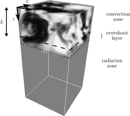
Figure 2.— Illustration of the computational domain. The white and black coloring respectively indicates positive and negative values of $u_{x}$ at time $t=t_{0}$ in the simulation described in Section 4.2. The thickness of the convective layer, $L$, is fixed, but convective overshoot causes the shear flow to extend into the radiation zone.

As in the study of Brummell et al. (2002), we choose a vertical profile for the thermal conductivity, $k(z)$, and impose a uniform vertical heat flux $H$ at the bottom of the domain. We choose $k(z)$ and $H$ such that the radiative temperature gradient is subadiabatic in the lower part of the domain, and superadiabatic (i.e., convectively unstable) in the upper part of the domain. This naturally leads to the formation of a lower radiation zone and an upper convection zone. In all the computations presented here the box size is $2L\times 2L\times 4L$, where $L$ is the thickness of the convection zone. The radiation zone is chosen to be three times thicker than the convection zone in order to minimize the influence of the bottom boundary on the dynamics. The numerical resolution is typically $100\times 100\times 400$; we require greater resolution in the vertical direction in order to accurately resolve any boundary layers that form at the interface between the convection and radiation zones. The top and bottom boundaries of the domain are both impenetrable and stress-free. We impose constant temperature $T_{0}$ at the top of the domain, $z=0$, and a constant heat flux at the bottom. Initially, the fluid is at rest and in hydrostatic balance with uniform vertical heat flux throughout, and has pressure $p_{0}$ and density $\rho_{0}$ at the upper boundary $z=0$. The ideal gas equations are nondimensionalized using the thickness of the convective layer, $L$, as the lengthscale, and $L/c$ as the timescale, where $c=\sqrt{p_{0}/\rho_{0}}$ is the isothermal sound speed at the top of the domain. The temperature, $T$, pressure, $p$, and density, $\rho$, are nondimensionalized using $T_{0}$, $p_{0}$, and $\rho_{0}$, respectively. The dimensionless ideal gas equations then take the form

$$\rho\left(\frac{\partial}{\partial t}+\bm{u}\cdot\bm{\nabla}\right)\bm{u}-2\Omega\rho\,\mathbf{e}_{z}\times\bm{u} =-\bm{\nabla}p+g\rho\mathbf{e}_{z}+2\mu\bm{\nabla}\cdot\mathbf{D}+F\mathbf{e}_{x}$$ (2)

$$\left(\frac{\partial}{\partial t}+\bm{u}\cdot\bm{\nabla}\right)\rho =-\rho\bm{\nabla}\cdot\bm{u}$$ (3)

$$p =\rho T$$ (4)

$$\rho T\left(\frac{\partial}{\partial t}+\bm{u}\cdot\bm{\nabla}\right)\ln(p^{1/\gamma}/\rho) =\bm{\nabla}\cdot\left(k(z)\bm{\nabla}T\right)+\frac{\gamma\!-\!1}{\gamma}2\mu\mathbf{D}:\mathbf{D},$$ (5)

where $\gamma=5/3$ is the ratio of specific heats, the constants $\Omega$ and $g$ are the dimensionless rotation rate and gravitational acceleration, and $\mathbf{D}$ is the deviatoric rate-of-strain tensor,

$$D_{ij}=\frac{1}{2}\frac{\partial u_{i}}{\partial x_{j}}+\frac{1}{2}\frac{\partial u_{j}}{\partial x_{i}}-\frac{1}{3}\bm{\nabla}\cdot\bm{u}\,\delta_{ij}.$$ (6)

We have also introduced the dimensionless dynamic viscosity $\mu$ and thermal conductivity $k$, which are related to their dimensional counterparts, $\mu^{\star}$ and $k^{\star}$ say, by

$$\mu=\frac{\mu^{\star}}{\rho_{0}cL}\hskip 28.45274pt\mbox{and}\hskip 28.45274ptk=\frac{k^{\star}\!/C_{p}}{\rho_{0}cL},$$ (7)

where $C_{p}$ is the specific heat capacity. We take $\mu$ to be constant throughout the domain, whereas for $k$ we impose a vertical profile of the form

$$k(z)\;=\;\frac{k_{1}}{1+\exp(20(z-1))}\;+\;\frac{k_{2}}{1+\exp(20(1-z))},$$ (8)

so that $k=k_{1}$ in the upper layer, $z<1$, and $k=k_{2}>k_{1}$ in the lower layer, $z>1$, the change occurring across a region of dimensionless thickness $\simeq 0.1$. The bottom of the convection zone is therefore fixed at $z=1$, but convective motions are able to overshoot into the radiation zone.

We write the three components of the velocity field as $\bm{u}=(u_{x},u_{y},u_{z})$. In our horizontally-periodic Cartesian model, differential rotation corresponds to any $x$-averaged flow in the $x$ direction, and angular momentum is essentially equivalent to azimuthal momentum, $\rho u_{x}$. Because our computational domain is horizontally symmetric, the Reynolds stresses in the convective layer are not able to drive any mean differential rotation. In order to mimic the generation of differential rotation in the solar convection zone, we add a volume forcing term to the $x$ component of the momentum equation (2),

$$F=\lambda(z,t)\rho(u_{\rm T}(y,z,t)-u_{x}).$$ (9)

The effect of the forcing term is to push the flow toward a prescribed “target” shear flow $u_{\rm T}$ at a rate $\lambda$. We have chosen to consider a situation analogous to the thought-experiment of Spiegel & Zahn (1992), in which the radiation zone is initially in uniform rotation despite the presence of differential rotation in the convection zone. We therefore take $\lambda$ to be constant initially, $\lambda=\lambda_{0}$, and the target velocity $u_{\rm T}$ is taken to be

$$u_{\rm T}\;=\;\frac{u_{0}(1-z)\sin(\pi y)}{1+\exp(20(z-1))},$$ (10)

which tends to zero at depths $z>1$. We thereby suppress differential rotation in the radiation zone and drive differential rotation in the convection zone. By suppressing differential rotation in the radiation zone we also prevent the burrowing of meridional circulations, which are tied to the differential rotation through the balances described in Section 1.2.

In all the computations presented here we take $\lambda_{0}=2\Omega$, so that the forcing rate matches the rotation rate, and $u_{0}=2\Omega/\pi$, so that the shearing timescale is comparable to the rotation period. The Rossby number $\Omega^{-1}\partial u_{\rm T}/\partial y$ is therefore of order unity, and so the differential rotation is somewhat stronger than that observed in the Sun and most solar-type stars (e.g., Reiners, 2006). By forcing a strong differential rotation, we can study the nonlinear effects of finite Rossby number, which were neglected in most of the idealized models reviewed in Section 1.3. Once the differential rotation reaches a statistically steady state, at $t=t_{0}$ say, the forcing parameters are changed to

$$\lambda\; =\;\frac{\lambda_{0}}{1+\exp(20(z-1))}$$ (11)

and $$u_{\rm T}\; =\;u_{0}(1-z)\sin(\pi y)\hskip 56.9055pt\mbox{for $t>t_{0}$}$$ (12)

so that $\lambda$ tends to zero at depths $z>1$. This means that the suppressive forcing is switched off below the convection zone for $t>t_{0}$, allowing the differential rotation to propagate into the interior, if the dynamics so dictate.

3. CHOICE OF PARAMETERS

The burrowing described in Section 1.3 is expected to occur only under specific parameter conditions, which are difficult to achieve in a computational model. The relevant parameter regime can be characterized as a hierarchy of timescales in the radiation zone:

acoustic time

$\ll$

buoyancy time

$\ll$

rotation time

$\ll$

Eddington–Sweet time

$\ll$

viscous time

(e.g., Clark, 1973). In terms of our dimensionless parameters, these conditions can be expressed as

$$1\;\;\ll\;\;\frac{1}{N}\;\;\ll\;\;\frac{1}{2\Omega}\;\;\ll\;\;\left(\frac{N}{2\Omega}\right)^{\!2}\frac{W^{2}}{k_{2}/\rho}\;\;\ll\;\;\frac{W^{2}}{\mu/\rho}$$ (13)

where $N$ is the dimensionless buoyancy frequency,

$$N^{2}=\frac{g^{2}}{T}\left(\frac{\gamma\!-\!1}{\gamma}-\frac{1}{g}\frac{\mathrm{d}T}{\mathrm{d}z}\right),$$ (14)

and $W$ is a characteristic horizontal lengthscale, which is of order unity in our Cartesian model. We note in particular that the viscous time (i.e., the timescale for viscous diffusion across the domain) must exceed the Eddington–Sweet time. This condition can be expressed as a constraint on the Prandtl number $\mu/k_{2}$ within the radiation zone:

$$\mu/k_{2}\;\;\ll\;\;\left(\frac{2\Omega}{N}\right)^{\!2}.$$ (15)

This constraint is particularly stringent because the second inequality in Equation (13) implies that the right-hand side of Equation (15) is $\ll 1$. Following Garaud & Acevedo-Arreguin (2009) we introduce the dimensionless parameter

$$\sigma=\frac{N}{2\Omega}\sqrt{\dfrac{\mu}{k_{2}}}$$ (16)

in order to express condition (15) more succinctly as $\sigma\ll 1$. If this condition is not met then viscous transport of angular momentum dominates the transport by meridional flows (Clark, 1973; Benton & Clark, 1974, §3.4), and we expect the burrowing of the meridional circulation to be less efficient. For example, in the laminar, steady-state model of Garaud & Acevedo-Arreguin (2009), cases with $\sigma>1$ have meridional circulations that decay exponentially beneath the convection zone, across a boundary layer similar to that described by Barcilon & Pedlosky (1967) (see also Lineykin, 1955).

For any solar-type star at the start of the main-sequence, condition (15) holds throughout the radiation zone, but as the star spins down through magnetic braking, this condition may cease to hold in the most strongly stably stratified regions. In the solar interior, for example, condition (15) holds only within the outer part of the radiation zone (Garaud & Acevedo-Arreguin, 2009) and a very small region at the center.

Computational limitations make it difficult to achieve the “low-sigma” regime described by condition (15) in a numerical model. If the rotation rate $\Omega$ and buoyancy frequency $N$ take realistic stellar values, then the Prandtl number $\mu/k_{2}$ must be extremely small, which requires very high spatial resolution. For this reason, all global simulations of the solar interior have been performed in the “high-sigma” regime, $\sigma>1$ (e.g., Rogers, 2011; Brun et al., 2011; Strugarek et al., 2011). It is therefore important to test whether the behavior of meridional flows in nonlinear numerical simulations depends on $\sigma$ in the same manner as is predicted by laminar models. In order to reach a parameter regime with $\sigma<1$, we have chosen here to use a local model, and to adopt more modest values for $\Omega$ and $N$, while still preserving the ordering of timescales given by (13).

The code of Brummell et al. (2002) requires the specification of six dimensionless input parameters, which we take to be:

• the values $k_{1}$ and $k_{2}$ of the thermal conductivity in the convection and radiation zones;

• the dynamic viscosity $\mu$;

• the gravitational acceleration $g$;

• the rotation rate $\Omega$;

• the heat flux $H=k_{2}\partial T/\partial z$ at the bottom of the domain.

For any particular choices of $H$ and $k_{1}$ we can choose values for the remaining parameters in order to satisfy the four constraints in (13); different choices for $H$ and $k_{1}$ correspond to different degrees of compressibility and convective overshoot. In practice, we choose values for $H$ and $k_{1}$ such that the pressure scale height is comparable to the height of the domain, and such that convective overshoot extends a distance of order $0.1$ below the base of the convection zone (see

Figure 3.— )

, as is thought to be typical for solar-type stars (e.g., Brummell et al., 2002; Rempel, 2004).

4. RESULTS

In the following sections we present results from four simulations performed in different parameter regimes. The first simulation, Case 0, differs from the others in that the conductivity of the upper layer, $k_{1}$, was chosen to make that layer adiabatic, and hence marginally stable to convection. The flow in this simulation therefore remains laminar, with no convection or internal wave generation, and so we expect the results to follow the predictions of the laminar models summarized in Section 1.3. Case 1 has the same parameters as Case 0 for the lower layer, but has a smaller conductivity $k_{1}$ in the upper layer, so that the upper layer is convectively unstable. Both Case 0 and Case 1 obey the ordering of timescales in (13), and so both have $\sigma<1$; we will refer to this as the “low-sigma regime”.

Case 2 and Case 3 both have a larger viscosity $\mu$ and smaller thermal conductivity $k$ throughout the domain, relative to Case 1, such that $\sigma>1$; we will refer to this as the “high-sigma regime”. Case 2 has a larger viscosity and conductivity than Case 3, but both have the same Prandtl number $\mu/k$, equal to 0.24 in the lower layer, $z>1$. In both cases the heat flux $H$ was chosen so that the stratification profile, and hence the buoyancy frequency $N$, matches that of Cases 0 and 1. Case 2 is only weakly convective, because of its relatively high viscosity, whereas Case 3 is more strongly convective, because of its low thermal conductivity.

In each simulation the dimensionless rotation rate and gravitational acceleration were taken to be $\Omega=9.6\times 10^{-3}$ and $g=0.24$ respectively. The other parameters, and relevant timescales, are listed in Table 1. For reference, Table 1 also lists characteristic values for the same dimensionless timescales in the solar interior, based on the values at $0.7R_{\odot}$ reported by Gough (2007). To allow the most direct comparison with the numerical simulations, the solar timescales are calculated using the lengthscale $W=0.7R_{\odot}\simeq 4.9\times 10^{10}$ cm, and quoted in units of $L/c$, where $L=1.4\times 10^{9}$ cm is one quarter of the pressure scale height and $c=\sqrt{p/\rho}\simeq 1.8\times 10^{7}$ cm s^-1 is the isothermal sound speed.

Table 1Parameters of each simulation, and corresponding solar parameters

Case	$10^{4}k_{1}$	$10^{4}k_{2}$	$10^{4}\mu$	$10^{4}H$	$\dfrac{1}{N}$	$\dfrac{1}{2\Omega}$	$\left(\dfrac{N}{2\Omega}\right)^{\!2}\dfrac{W^{2}}{k_{2}/\rho}$	$\dfrac{W^{2}}{\mu/\rho}$	$\sigma$
0	15.1	24.1	0.145	1.4	11	52	1.0$\times 10^{4}$	7.9$\times 10^{4}$	0.36
1	14.5	24.1	0.145	1.4	11	52	1.0$\times 10^{4}$	7.9$\times 10^{4}$	0.36
2	5.12	8.53	2.05	0.51	11	52	2.9$\times 10^{4}$	0.56$\times 10^{4}$	2.27
3	1.93	3.22	0.774	0.19	11	52	7.6$\times 10^{4}$	1.5$\times 10^{4}$	2.27
Sun	$\cdots$	$\cdots$	$\cdots$	$\cdots$	16	2400	4.8$\times 10^{16}$	1.1$\times 10^{18}$	0.21

Note. — The last five columns give approximate values for the dimensionless timescales in Equation (13) and the value of $\sigma$, calculated using the time-averaged density $\rho$ and buoyancy frequency $N$ below the overshoot region.

4.1. Case 0: The Low-Sigma Regime, without Convection

In this case the upper layer, $0<z<1$, is non-convective, and so we expect the dynamics to follow the predictions of the laminar models discussed in Section 1.3. Figure 4 shows the steady azimuthal shear and meridional flow at $t=t_{0}$. By this time the flow has reached a steady state with a large-scale azimuthal shear and meridional circulation in the upper layer. Both the shear and circulation extend slightly into the lower layer, to an extent that depends on the rate at which the target velocity $u_{\rm T}$ tends to zero for $z>1$, but for $z>1.3$ the flow is exponentially weak. We note that the azimuthal shear $u_{x}$ does not exactly match the target shear flow $u_{\rm T}$ given by Equation (10). In the steady state, the “residual” forcing $\lambda_{0}\rho(u_{\rm T}-u_{x})$ is balanced primarily by the azimuthal component of the Coriolis force, $2\Omega\rho u_{y}$, and this balance determines the strength of the meridional flow within the upper layer. This is an example of the process referred to as gyroscopic pumping in Section 1.2. Within the upper layer, the downwelling portion of the meridional circulation is stronger than the upwelling portion. This asymmetry is a symptom of the Rossby number being of order unity, and is therefore less apparent in the lower layer, where the shear is weaker.

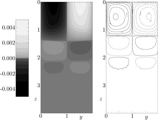
Figure 4.— Shear flow $u_{x}$ (left panel) and meridional streamlines (right panel) from Case 0, averaged in $x$ at time $t=t_{0}$. The meridional streamlines are drawn as contours of a streamfunction $\psi$, which was computed assuming that $\bm{\nabla}\cdot\rho\bm{u}=0$. Solid and dashed contours indicate anti-clockwise and clockwise circulation respectively. Contour levels for $u_{x}$ and $\psi$ are cubically spaced to show more detail in the radiation zone, where the flows are weakest.

At $t=t_{0}$ the forcing is switched off below $z=1$, allowing the flow of the upper layer to propagate into the lower, stably stratified layer. The sudden imbalance of forces also generates a spectrum of internal waves. Figure 10 shows time averages of the azimuthal shear and meridional flow, averaged over one rotation period, at regular intervals after $t=t_{0}$. The time averaging filters out most of the internal wave modes, making the long-time evolution more visible. From $t=t_{0}$ onwards, the meridional circulation of the upper layer begins to burrow into the lower layer, as indicated by the increased vertical extent of the main meridional circulation cell in the lower panel of

Figure 5.— .

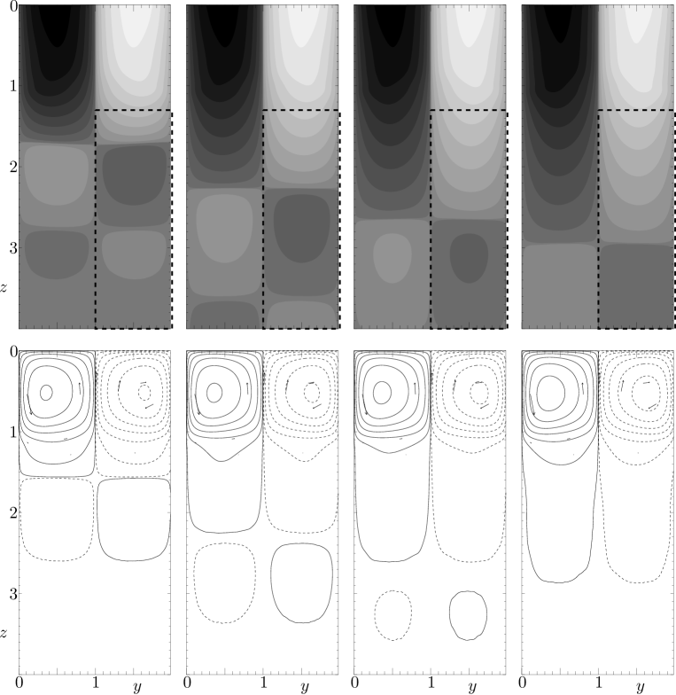
Figure 8.— Shear flow and meridional streamlines from Case 0 averaged over one rotation period for successive times $t>t_{0}$, using the same contour levels as in

Figure 9.— .

The time averages were taken over the intervals $\Delta t_{1}$, $\Delta t_{2}$, $\Delta t_{3}$, and $\Delta t_{4}$ indicated in

Figure 10.— .

The dashed box in the upper panels indicates the control volume $V$ used in Equation (18).

The mean azimuthal shear also propagates into the lower layer, at approximately the same rate, suggesting that the transport of angular momentum is the result of advection by the meridional flow, as expected for a laminar flow at these parameter values. To verify this, we first use the mass conservation equation (3) to write the azimuthal component of the momentum equation (2) as

$$\frac{\partial}{\partial t}(\rho u_{x})=-2\Omega\rho u_{y}-\bm{\nabla}\cdot(\rho u_{x}\,\bm{u})+\mu\nabla^{2}u_{x}+F.$$ (17)

After integrating over a fixed volume $V$, and employing the divergence theorem, we obtain

$$\frac{\mathrm{d}}{\mathrm{d}t}\int_{V}\!\mathrm{d}V\rho u_{x}\;=\;\underbrace{-\;\;2\Omega\int_{V}\!\mathrm{d}V\rho u_{y}}_{\rm Coriolis}\;\underbrace{-\;\int_{\partial V}\!\mathrm{d}\mathbf{S}\cdot\bm{u}\,\rho u_{x}}_{\rm inertial}\;\underbrace{+\;\;\mu\int_{\partial V}\!\mathrm{d}\mathbf{S}\cdot\bm{\nabla}u_{x}}_{\rm viscous}\;\underbrace{+\;\int_{V}\!\mathrm{d}VF}_{\rm forcing},$$ (18)

where $\partial V$ represents the boundary of $V$, and where $\mathrm{d}\mathbf{S}$ is the area element directed outward. In order to verify that the burrowing meridional circulation seen in the lower panel of

Figure 11.— i

s responsible for the propagation of the shear flow into the interior, we have computed each integral in Equation (18) for the control volume $V$ indicated by the dashed box in the upper panel of

Figure 12.— .

The result, after taking a time average over one rotation period, is plotted in

Figure 13.— .

The left panel of

Figure 14.— s

hows that, whereas the azimuthal momentum in the upper layer adjusts to a new equilibrium after only a few rotation periods, the lower layer adjusts on a much longer timescale. The right panel shows that the long-time transport of azimuthal momentum into the lower layer can be attributed almost entirely to the azimuthal Coriolis force arising from the mean meridional flow, which corresponds to advection of angular momentum viewed in our rotating frame.

Figure 16.— Left panel: The solid line shows the total azimuthal momentum $\int\mathrm{d}V\rho u_{x}$ in the dashed box indicated in

Figure 17.— ,

averaged over one rotation period. For comparison, the dashed line shows the total azimuthal momentum in the region above the dashed box. Right panel: The four terms contributing to the right-hand side of Equation (18), and their total, each averaged over one rotation period. The length of one rotation period $2\pi/\Omega$ is indicated on the plot. The total duration plotted corresponds to about half of the Eddington–Sweet time.

As a further illustration of the relative contributions of the different processes to the net transport of angular momentum, in

Figure 18.— w

e present vertical cross-sections of each term on the right-hand side of Equation (17), after averaging in azimuth and over the time interval $\Delta t_{1}$ indicated in

Figure 19.— .

Within the upper layer, the Coriolis and forcing terms are approximately in balance, and the strength of the meridional flow is determined by gyroscopic pumping. Within the lower layer, the Coriolis term dominates all others, leading to the evolution of the differential rotation seen in

Figure 20.— .

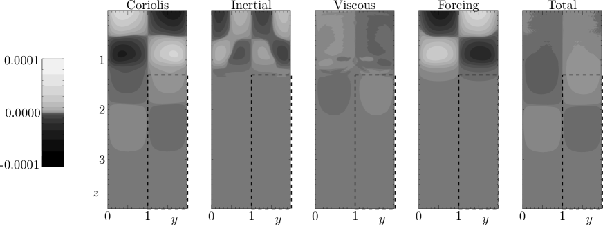
Figure 22.— Vertical cross-sections of each term on the right-hand side of Equation (17), and their total, averaged in azimuth and over the time interval $\Delta t_{1}$ indicated in

Figure 23.— .

The contour levels are cubically spaced, as indicated by the colorbar on the left. Throughout the control volume $V$, indicated by the dashed box, the Coriolis term provides the dominant contribution to the total angular momentum transport.

Within this layer, the strength of the meridional flow is determined by meridional force balance and local thermal equilibrium, as anticipated by the Vogt–Eddington argument of Section 1.2, and is therefore roughly proportional to the vertical gradient of the angular velocity, i.e., to $\partial u_{x}/\partial z$ in our Cartesian geometry. This explains why the differential rotation and meridional circulation propagate at the same rate, and also why the strength of the meridional flow, and hence the rate of burrowing, decays over time. The results in this case are entirely consistent with the laminar models described in Section 1.3.

4.2. Case 1: The Low-Sigma Regime, with Convection

We now study the effects of turbulent convective overshoot and internal waves on the burrowing of meridional flows. In Case 1, unlike Case 0, the upper layer, $0<z<1$, is convectively unstable, and has an rms Reynolds number $\simeq 550$. The turbulent motions in this layer continually generate internal waves, which propagate into the lower, stably stratified layer. Nevertheless, for times $t\leqslant t_{0}$ the time-averaged shear and meridional circulation are confined to the upper layer, as in Case 0. Motions in the lower layer, $z>1$, are suppressed by the forcing in that region.

At $t=t_{0}$ the forcing is switched off in the lower layer. Figure 30 shows the mean shear and meridional flow, averaged over two rotation periods, at regular intervals after $t=t_{0}$, using the same contour levels as

Figure 24.— .

As in Case 0, the shear and meridional circulation both extend progressively deeper into the lower layer over time, though in a much less regular fashion than in Case 0. In any snapshot of the meridional flow, the mean circulation is completely dominated by internal wave motions, but after averaging over two rotation periods we observe a similar mean circulation to that in

Figure 25.— .

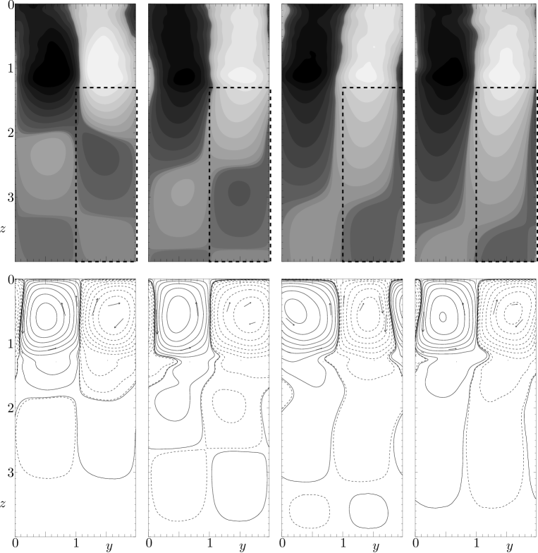
Figure 28.— Shear flow and meridional streamlines from Case 1, averaged over two rotation periods for times $t>t_{0}$. Time averages were taken over the intervals indicated in

Figure 29.— .

The contour levels are the same as in

Figure 30.— .

In

Figure 31.— w

e show the evolution of the azimuthal momentum in the volume indicated by the dashed box in

Figure 32.— ,

as well as the terms contributing to the right-hand side of Equation (18) for this volume. (This figure is equivalent to

Figure 33.— i

n Section 4.1.) Despite the presence of internal waves, we find that the mean meridional circulation dominates the long-time transport of azimuthal momentum into the radiative layer, as in Case 0 for which the flow was laminar.

Figure 36.— Same plots as

Figure 37.— ,

but for Case 1 and averaged over two rotation periods. The scale in the right-hand panel is larger than in

Figure 38.— .

The inertial contributions to the momentum transport, which are associated with waves and turbulent fluctuations, are larger than in Case 0, but the Coriolis force from the mean meridional flow remains dominant in the long term, leading to the overall increase in azimuthal momentum shown by the solid line in the left panel. The dimensionless Eddington–Sweet time in this case is $\simeq 10^{4}$.

Although there is qualitative agreement between the results of Case 0 and Case 1, we note that they differ in certain respects. In particular, the propagation of the shear into the lower layer does not proceed monotonically, as can be seen in the left panel of

Figure 39.— (

cf.

Figure 40.— )

, indicating that the burrowing process does not act continuously throughout the simulation. Perhaps more surprising, however, is that the overall rate of burrowing is faster in Case 1 than in Case 0. These differences between Case 0 and Case 1 can be attributed to differences in the profile of $u_{x}$ within the upper layer in the two cases. In Case 0, $u_{x}$ is strongest close to the upper boundary, $z=0$, where the forcing is strongest. In Case 1, $u_{x}$ is highly time-dependent, but generally strongest close to the interface $z=1$ (see

Figure 41.— )

. Therefore the amplitude of $u_{x}$ at the top of the radiation zone is generally stronger in Case 1, but varies significantly in time, producing a burrowing that is more rapid overall, but very irregular. The occasional reversals in the sign of the momentum transport in

Figure 42.— (

e.g., for $2000\leqslant t\leqslant 3000$) correspond to the periods when $u_{x}$ at the interface is weakest. The variations in $u_{x}$ in the upper layer are quasi-periodic, with a timescale of several rotation periods, and may possibly be the result of an inertial mode trapped within the convection zone. (An inertia–gravity oscillation within the radiation zone, on the other hand, would necessarily have a period of less than half the rotation period, because $N>2\Omega$.) In that case the oscillation relies on the artificial local geometry of our model, and would not be present in a global model. Finally, we note that during the phases when burrowing does occur, the transport of angular momentum throughout the radiation zone is qualitatively similar to that in Case 0. This is illustrated in

Figure 43.— ,

in which we plot vertical cross-sections of each term on the right-hand side of Equation (17), averaged in azimuth and over the interval $\Delta t_{1}$ indicated in

Figure 44.— .

(This figure is equivalent to

Figure 45.— i

n Section 4.1.) Although there is a non-zero contribution from the inertial and viscous terms, the main contribution comes from the Coriolis term, and the overall transport of angular momentum in the radiation zone resembles that in Case 0.

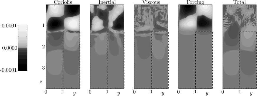
Figure 48.— Same plots as

Figure 49.— ,

but for Case 1 and averaged over the time interval $\Delta t_{1}$ indicated in

Figure 50.— .

As in Case 0, the Coriolis term provides the dominant contribution to the total angular momentum transport in the radiation zone.

4.3. Case 2: The High-Sigma Regime; High Viscosity

In Case 2 the viscous diffusion timescale is shorter than the Eddington–Sweet timescale, primarily because the viscosity is larger than in Cases 0 and 1, and so $\sigma>1$. The rotation rate $\Omega$ and stratification profile in the radiation zone are the same as in Cases 0 and 1.

Because of the increased viscosity, in this case the upper layer is only weakly convective, and consequently the mean flows are more clearly defined. Most of the kinetic energy in the upper, convective layer is associated with the mean azimuthal shear flow, rather than with convective motions. The mean azimuthal shear and meridional flow at successive times $t>t_{0}$ are plotted in

Figure 51.— ,

using the same contour levels as in Figures 10 and 30. We find that the convection zone’s azimuthal shear propagates progressively deeper into the radiation zone, as in Cases 0 and 1, but that meridional flows within the radiation zone remain confined to a thin layer below the bottom of the convection zone. The convection zone’s meridional circulation does not burrow significantly, and instead a weak counter-circulating meridional cell is established at the top of the radiation zone (cf. Figures 10 and 30).

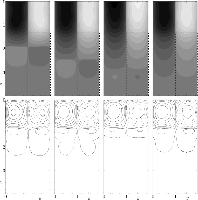
Figure 53.— Shear and meridional flow from Case 2, averaged over one rotation period for times $t>t_{0}$. Time averages were taken over the intervals indicated in

Figure 54.— .

Contour levels are the same as in Figures 10 and 30.

Figure 57 shows the equivalent of Figures 17 and 38 for Case 2. In this case, we find that the propagation of shear into the radiation zone is caused primarily by viscous diffusion. After about one viscous diffusion time, a roughly steady state is achieved in which the viscous force is balanced by the Coriolis force. We note that the Coriolis force in this case has the opposite sign than in Cases 0 and 1, so transport of azimuthal momentum by the mean meridional flow acts to oppose (but not prevent) the propagation of the convection zone’s shear into the radiation zone. This is a consequence of the counter-circulating meridional cell visible in

Figure 55.— ,

as demonstrated by

Figure 56.— ,

which shows vertical cross-sections equivalent to those of Figures 23 and 50 for Case 2. The lack of burrowing of the meridional circulation in this case is consistent with the predictions of laminar models with $\sigma>1$, as discussed in Section 3.

Figure 57.— Same plots as Figures 17 and 38, but for Case 2. The plots have been averaged over one rotation period. In this case the viscous term is dominant, and the Coriolis term takes the opposite sign. The total duration plotted corresponds to about one viscous diffusion time.

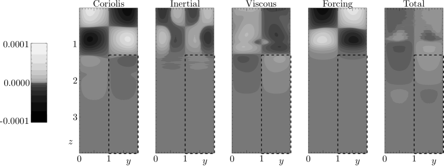
Figure 59.— Same plots as Figures 23 and 50, but for Case 2, and averaged over the time interval $\Delta t_{1}$ indicated in

Figure 60.— .

In this case the viscous term causes the convection zone’s azimuthal shear to propagate into the radiation zone. The Coriolis term has the opposite sign to the viscous term, and a smaller amplitude overall.

4.4. Case 3: The High-Sigma Regime; Low Thermal Conductivity

Case 3 has the same values of $\Omega$, $N$, and $\sigma$ as Case 2, but the viscosity and thermal conductivity are both smaller than in Case 2. As a result the upper layer is more strongly convective, with an rms Reynolds number $\simeq 60$. Although this Reynolds number is significantly lower than that of Case 1, we find that internal waves are generated with a larger amplitude in this case than in Case 1. We attribute this to the lower value of the thermal conductivity in this case, which reduces the damping of internal waves. In fact, we find that a standing gravity mode is excited in the lower layer, which slowly grows in amplitude during the simulation. The existence of this mode is dependent on the artificial lower boundary of the computational domain, and so we end the simulation at the point where the amplitude of this mode becomes large enough to significantly affect the dynamics (at around $t=t_{0}+4000$).

Figure 63 shows the mean azimuthal shear and meridional flow at successive times $t>t_{0}$, using the same contour values as Figures 10, 30, and 54. Despite the presence of internal waves, the mean flow exhibits similar behavior to Case 2. The meridional circulation driven in the convection zone turns over at only a short depth within the radiation zone, and a counter-rotating meridional cell forms beneath, though with a more complicated structure than in Case 2. Meanwhile, the convection zone’s shear propagates monotonically into the interior.

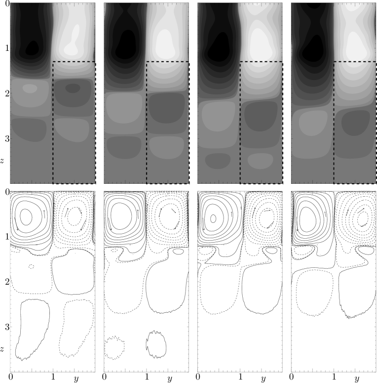
Figure 62.— Shear and meridional flow from Case 3, averaged over one rotation period for times $t>t_{0}$. Time averages were taken over the intervals indicated in

Figure 63.— .

Contour levels are the same as in Figures 10, 30, and 54.

Figure 64 shows the equivalent of Figures 17, 38, and 57 for Case 3. As in Case 2, we find that the propagation of shear into the radiation zone is caused primarily by viscous diffusion, although the relative contributions from inertial and Coriolis forces are larger than in Case 2.

Figure 64.— Same plots as Figures 17, 38, and 57, but for Case 3. The plots have been averaged over one rotation period. The viscous term is dominant, as in Case 2, until $t\simeq t_{0}+3000$. After this time the inertial contribution from a standing gravity mode becomes comparable to the viscous term.

In contrast to Case 2, however, the Coriolis term has the same sign as the viscous term, at least for times $t\lesssim 2500$. This is because the convection zone’s meridional circulation, shown in

Figure 65.— ,

manages to burrow a short distance into the radiation zone, as illustrated by

Figure 66.— ,

which shows the equivalent of Figures 23, 50, and 60 for Case 3, averaged over the time interval $\Delta t_{2}$ indicated in

Figure 67.— .

A similar result was obtained by Garaud & Acevedo-Arreguin (2009) in a steady-state model of the solar interior; they found that, when $\sigma>1$, meridional circulations that are gyroscopically pumped within the convection zone extend a distance of order $W/\sigma$ into the radiation zone, where $W$ is the horizontal lengthscale of the circulation, which in our model is of order unity.

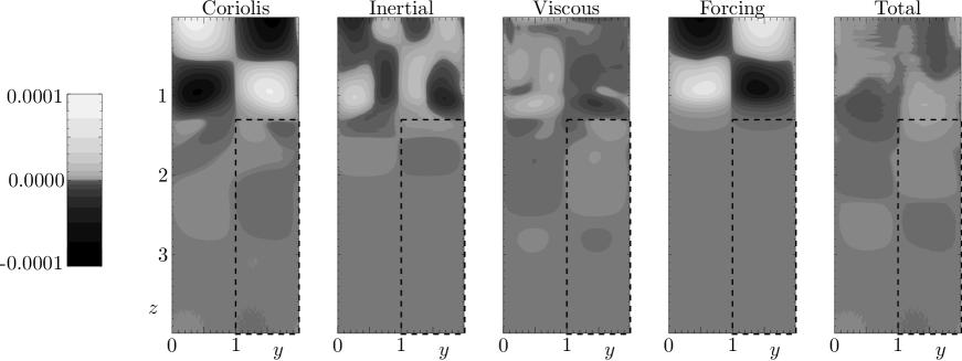
Figure 69.— Same plots as Figures 23, 50, and 60, but for Case 3, and averaged over the time interval $\Delta t_{2}$ indicated in

Figure 70.— .

As in Case 2, the viscous term is dominant throughout most of the radiation zone, but in this case the Coriolis and inertial terms also contribute to the propagation of the convection zone’s shear within a thin layer at the top of the radiation zone.

5. SUMMARY AND CONCLUSIONS

This paper presents the first 3D, self-consistent, and nonlinear study of meridional flows in the parameter regime described by Clark (1973), which is the relevant parameter regime for the radiative zones of many solar-type stars. In this regime the Eddington–Sweet time is shorter than the viscous time; the ratio of these timescales is determined by the dimensionless parameter $\sigma$ defined in Equation (16). We have considered four separate cases: two in the “low-sigma” regime and two in the “high-sigma” regime. Our results indicate that the underlying long-time dynamical picture of angular momentum transport predicted by laminar models applies even under more realistic conditions, including the presence of overshooting from the neighboring turbulent convection zone, and the internal waves that this generates.

In Cases 0 and 1, which have $\sigma<1$, angular momentum transport is dominated in the long term by advection by meridional flows, and the meridional circulation driven in the convection zone burrows (i.e., extends progressively downward) into the radiation zone on the Eddington–Sweet timescale, carrying the differential rotation of the convection zone with it. The burrowing is more irregular in Case 1 than in Case 0, as a result of angular momentum transport by turbulence and internal waves. In Cases 2 and 3, which have $\sigma>1$, viscous stresses dominate the transport of angular momentum in the radiation zone, although there is also a significant contribution from internal waves in Case 3. In these two cases the meridional circulation driven in the convection zone extends only a short distance into the radiation zone. The differential rotation of the convection zone still propagates into the radiation zone, but by viscous diffusion rather than by meridional advection.

It should be borne in mind that the simulations presented here are at most weakly turbulent, in comparison with real stellar convection. It may be that under the more turbulent conditions characteristic of real stellar interiors angular momentum transport is dominated by shear-driven turbulence or internal wave breaking, as argued for instance by Zahn (1992). If that is the case then our results may not be applicable to real stars. However, our results should certainly be applicable to previous global-scale simulations of the solar interior, including those of Rogers (2011), Brun et al. (2011), and Strugarek et al. (2011). We note that these simulations were all performed in the “high-sigma” regime in which we found that angular momentum transport is dominated by viscous stresses. All of these global models have $\sigma\simeq 200$ close to the top of the radiation zone (although in the model of Strugarek et al. (2011) $\sigma$ drops to around to 20 deeper within the radiation zone). In each of these simulations it was indeed found that viscous stresses contribute at leading order to the transport of angular momentum within the radiation zone. The pattern of meridional flows found in these simulations is also rather similar to that which we observe in our simulations with $\sigma>1$ (Figures 54 and 63), and no burrowing of the circulation was observed. In this situation we expect the transport of angular momentum between the convection and radiation zones to occur on a viscous timescale. This is indeed what Brun et al. (2011) and Strugarek et al. (2011) observe. Rogers (2011) reports that an apparently steady state is achieved in which viscous and Coriolis forces balance, and uniform rotation is preserved within the radiation zone. Based on our results, we suggest that this “steady state” is actually evolving slowly on a viscous timescale. We are now conducting global simulations in the low-sigma regime for comparison, to be presented in a forthcoming paper. Using a global model will also allow a more realistic study of the effects of internal waves, avoiding the difficulties encountered in Case 3.

All of the simulations presented here have the same rotation rate and stratification profile, and in each case the Prandtl number in the radiation zone is smaller than unity. Yet the strength and depth of the mean meridional circulations vary drastically between the four cases. This highlights the danger in modeling stellar interiors with numerical simulations that have, for example, realistic rotation and stratification but unrealistic diffusivities. Our results suggest that the ordering of dynamical timescales is of greater importance than the exact values of those timescales when considering angular momentum transport. Real stellar interiors are characterized by the same ordering as the simulations presented here, but with substantially greater separation.

If our results carry over to realistic stellar parameters then they have significant implications not only for angular momentum transport, but also for the transport of chemical elements and magnetic flux by meridional flows. In particular, the depth to which chemical elements are carried from the convection zone into the radiation zone will depend on the depth to which meridional circulations are able to burrow, and hence on the value of $\sigma$.

An important issue not addressed in the present work is the contribution of magnetic fields to angular momentum transport in stellar interiors. If magnetic fields act to suppress differential rotation in the radiation zone, then the burrowing of meridional flows will also be suppressed (Gough & McIntyre, 1998). In that case the role of the magnetic field is analogous to that of the forcing in the radiation zone in our model for $t<t_{0}$. Effects of magnetic fields will be addressed in future papers.

We thank Pascale Garaud, Gary Glatzmaier, Céline Guervilly, Michael McIntyre, and an anonymous referee for useful comments and suggestions. T.S.W. was supported by NSF CAREER grant 0847477. N.H.B. was supported by NASA grant NNX07AL74G and the Center for Momentum Transport and Flow Organization (CMTFO), a DoE Plasma Science Center. Numerical simulations were performed on NSF TeraGrid/XSEDE resources Kraken and Ranger, and the Pleiades supercomputer at University of California Santa Cruz purchased under NSF MRI grant AST-0521566.

References

- Barcilon & Pedlosky (1967) Barcilon, V., & Pedlosky, J. 1967, J. Fluid Mech., 29, 609
- Benton & Clark (1974) Benton, E. R., & Clark, A. 1974, Annu. Rev. Fluid Mech., 6, 257
- Brummell et al. (2002) Brummell, N. H., Clune, T. L., & Toomre, J. 2002, Astrophys. J., 570, 825
- Brun et al. (2011) Brun, A. S., Miesch, M. S., & Toomre, J. 2011, Astrophys. J., 742, 79
- Chaboyer & Zahn (1992) Chaboyer, B., & Zahn, J.-P. 1992, A&A, 253, 173
- Charbonneau & MacGregor (1993) Charbonneau, P., & MacGregor, K. B. 1993, Astrophys. J., 417, 762
- Charbonneau & Michaud (1988) Charbonneau, P., & Michaud, G. 1988, Astrophys. J., 334, 746
- Charbonnel & Talon (2005) Charbonnel, C., & Talon, S. 2005, Science, 309, 2189
- Clark (1973) Clark, A. 1973, J. Fluid Mech., 60, 561
- Clark (1975) Clark, A. 1975, Mémoires Société Royale des Sciences de Liège, 8, 43
- Couvidat et al. (2003) Couvidat, S., García, R. A., Turck-Chièze, S., Corbard, T., Henney, C. J., & Jiménez-Reyes, S. 2003, Astrophys. J., 597, L77
- Dikpati & Charbonneau (1999) Dikpati, M., & Charbonneau, P. 1999, Astrophys. J., 518, 508
- Eddington (1925) Eddington, A. S. 1925, The Observatory, 48, 73
- Eggenberger et al. (2005) Eggenberger, P., Maeder, A., & Meynet, G. 2005, A&A, 440, L9
- Elliott (1997) Elliott, J. R. 1997, A&A, 327, 1222
- Garaud & Acevedo-Arreguin (2009) Garaud, P., & Acevedo-Arreguin, L. A. 2009, Astrophys. J., 704, 1
- Garaud & Bodenheimer (2010) Garaud, P., & Bodenheimer, P. 2010, Astrophys. J., 719, 313
- Garaud & Brummell (2008) Garaud, P., & Brummell, N. H. 2008, Astrophys. J., 674, 498
- Gough (2007) Gough, D. 2007, in The Solar Tachocline, ed. D. W. Hughes, R. Rosner, & N. O. Weiss, 3
- Gough & McIntyre (1998) Gough, D. O., & McIntyre, M. E. 1998, Nature, 394, 755
- Haynes et al. (1991) Haynes, P. H., McIntyre, M. E., Shepherd, T. G., Marks, C. J., & Shine, K. P. 1991, J. Atmos. Sci., 48, 651
- Howard et al. (1967) Howard, L. N., Moore, D. W., & Spiegel, S. A. 1967, Nature, 214, 1297
- Kippenhahn (1963) Kippenhahn, R. 1963, Astrophys. J., 137, 664
- Lineykin (1955) Lineykin, P. C. 1955, Dokl. Akad. Nauk. SSSR, 101, 461
- McIntyre (2000) McIntyre, M. E. 2000, in Perspectives in Fluid Dynamics, ed. Batchelor, G. K., Moffatt, H. K. & Worster, M. G. (Cambridge: University Press), 557–624
- McIntyre (2002) McIntyre, M. E. 2002, in Meteorology and the Millennium, ed. R. P. Pearce, 283
- McIntyre (2007) McIntyre, M. E. 2007, in The Solar Tachocline, ed. D. W. Hughes, R. Rosner, & N. O. Weiss, 183
- Mestel (1953) Mestel, L. 1953, MNRAS, 113, 716
- Mestel (1999) Mestel, L. 1999, Stellar magnetism, no. 99 in International series of monographs on physics (Oxford: Clarendon)
- Miesch (2005) Miesch, M. S. 2005, Living Rev. Sol. Phys., 2, 1
- Pinsonneault (1997) Pinsonneault, M. 1997, Annu. Rev. Astron. Astrophys., 35, 557
- Reiners (2006) Reiners, A. 2006, A&A, 446, 267
- Rempel (2004) Rempel, M. 2004, Astrophys. J., 607, 1046
- Rogers (2011) Rogers, T. M. 2011, Astrophys. J., 733, 12
- Rüdiger & Kitchatinov (1997) Rüdiger, G., & Kitchatinov, L. L. 1997, Astron. Nachr., 318, 273
- Sakurai (1970) Sakurai, T. 1970, in IAU Colloq. 4: Stellar Rotation, 329
- Schatzman (1962) Schatzman, E. 1962, Annales d’Astrophysique, 25, 18
- Schatzman (1993) Schatzman, E. 1993, A&A, 279, 431
- Spiegel (1972) Spiegel, E. A. 1972, NASA Special Publication, 300, 61
- Spiegel & Zahn (1992) Spiegel, E. A., & Zahn, J.-P. 1992, A&A, 265, 106
- Strugarek et al. (2011) Strugarek, A., Brun, A. S., & Zahn, J.-P. 2011, A&A, 532, A34
- Sweet (1950) Sweet, P. A. 1950, MNRAS, 110, 548
- Vogt (1925) Vogt, H. 1925, Astron. Nachr., 223, 229
- Zahn et al. (1997) Zahn, J.-P., Talon, S., & Matias, J. 1997, A&A, 322, 320
- Zahn (1992) Zahn, J.-P. 1992, A&A, 265, 115