Holographic energy density on Hořava-Lifshitz cosmology

Abstract

In Hořava-Lifshitz cosmology we use the holographic Ricci-like cut-off for the energy density proposed by L. N. Granda and A. Oliveros and under this framework we study, through the cosmic evolution at late times, the sign change in the amount of non-conservation energy ($Q$) present in this cosmology. We revise the early stage (curvature-dependent) of this cosmology, where a term reminiscent of stiff matter is the dominant, and in this stage we find a power-law solution for the cosmic scale factor although $\omega=-1$. Late and early phantom schemes are obtained without requiring $\omega<-1$. Nevertheless, these schemes are not feasible according to what is shown in this paper. We also show that $\omega=-1$ alone does not imply a de Sitter phase in the present cosmology. Thermal aspects are revised by considering the energy interchange between the bulk and the spacetime boundary and we conclude that there is no thermal equilibrium between them. Finally, a ghost scalar graviton (extra degree of freedom in HL gravity) is required by the observational data.

I Introduction

The Hořava-Lifshitz (HL) cosmology Mukohyama2010 is a formalism generated from HL gravity (a possible candidate for quantum gravity?), which is a power-counting renormalizable gravity theory (expected to be renormalizable and unitary) that leads to modifications of Einstein’s general relativity at high energies producing novel features for considering cosmology. This formalism suffers from the lack of local Hamiltonian constraint and thus there is no a Friedmann equation here. Therefore, if a projectability condition is imposed (the lapse function is restricted being only time-dependent), then the Hamiltonian constraint becomes one global. This means that the Hamiltonian constraint in HL gravity is not a local equation but an equation integrated over a whole space and the projectability condition is compatible with the foliation preserving diffeomorphism (diffeomorphism invariance). In HL gravity, in addition to the tensor graviton, the theory exhibits an extra scalar degree of freedom called scalar graviton and, as we shall see, the role of this extra degree of freedom (which we ”characterize” by a $\eta$-parameter) will play an important role alongside parameters from the observational data.

In the present work we follow the philosophy developed in Kobayashi2009 , Section III. In particular, the claim cited there ”the global Hamiltonian constraint that $Q$ (amount of non-conservation energy) does not necessarily vanish in the local patch” is the main key of our work. In Mukohyama2010 and under this scope, it is shown that $Q$ is not zero today and only today we have $C_{0}/a^{3}$, that is, $\epsilon\left(t\right)=const/a^{3}$(according to the notation of Kobayashi2009 and MukohyamaWangMaartens2009 ).

In HL cosmology (described here in a Friedmann-Lemaitre-Robertson-Walker universe) we have a non-conservation equation for the cosmic fluid, and the sign change experienced by the amount of non-conservation energy through the cosmic evolution, treated in the present paper as the energy interchange between the bulk and the spacetime boundary and we mean by bulk the observable universe and by boundary its Hubble horizon. The thermal equilibrium between them will be discussed by using a holographic cut-off for the energy density and we will discuss also early and late phantom solutions obtained and its factibility in the present cosmology.

The paper is organized as follows: Considering the flat case in Section II, we inspect the sign change in the amount of non-conservation energy through the cosmic evolution by using the $q$-parameter (deceleration parameter) and a phantom solution is found without requiring $\omega<-1$. In Section III we use a $q(z)$-parametrization in order to visualize the sign change of the aforementioned $Q(z)$. In Section IV we use a $\omega(z)$-parametrization in order to complement the discussion on the sign change of $Q(z)$ done from Section III. In Section V we study the early limit of HL cosmology and we find a scheme with $\omega=-1$ where the Hubble parameter exhibits a power-law behavior and we find a phantom scheme in which also $\omega=-1$. In Section VI we analyze some thermal aspects under the idea of a sign change of $Q(z)$. Section VII is devoted to presents our conclusions. $G=c=1$ units will be used.

II Holographic Ricci-like on flat Hořava-Lifshitz cosmology

We consider the dynamic equation Mukohyama2010

$$\eta(2\dot{H}+3H^{2})=-\omega\rho,$$ (1)

where $\eta=(3\lambda-1)/2$ with $\lambda$ being a dimensionless parameter fixed by the diffeomorphism invariance of 4D general relativity (GR) and $0<\eta<1$ (ghost instability; ghost scalar graviton), $\eta<0$ or $\eta>1$ (non-ghost scalar graviton) and $\eta$ is fixed to $1$ in GR. $H$ is the Hubble parameter, $\omega=p/\rho$ being $p$ the pressure and $\rho$ the energy density and the dot means the temporal derivative. The non-conservation equation for the energy density is given by

$$\dot{\rho}+3H\left(1+\omega\right)\rho=-Q,$$ (2)

where $Q$ is the amount of non-conservation energy present in the model and the low energy limit can be recovered if $Q\longrightarrow 0$. We recall here that $Q$ comes from the theory (as an integration term in HL-cosmology) and not imposed by hand when, for example, interacting fluids are treated. Now, by considering $\rho$ as a dominant component (the unspoken components, if any, are negligible), we will interpret the sign change of $Q$ as energy transference between the bulk and the spacetime boundary.

Although under a different scope at the present work, in Xiao-Dong2013 we see observational evidence for $Q\left(0\right)>0$, namely decay of dark energy into dark matter. From our perspective, we can affirm something similar, that is, decay of energy from the bulk into the boundary of spacetime.

By introducing in (1) the holographic energy density model GrandaOliveros2008 , written in terms of the $q$-parameter defined by $q=-\left(1+\dot{H}/H^{2}\right)$,

$$\rho=3\left(\alpha H^{2}+\beta\dot{H}\right)=3\left[\alpha-\beta\left(1+q\right)\right]H^{2},$$ (3)

where $\alpha$ and $\beta$ are both positive dimensionless constant parameters Lepe2010 , we obtain

$$\eta\left[3-2\left(1+q\right)\right]=-3\omega\left[\alpha-\beta\left(1+q\right)\right].$$ (4)

And from this last expression, in addition to (2), it is straightforward to obtain

$$\frac{Q}{3H^{3}}=-2\eta\left[1-\frac{\alpha}{\eta}+\frac{\beta}{\eta}\left(1+q\right)\right]\left(q-\frac{1}{2}\right)$$

$$-\beta\left(1+z\right)\frac{dq}{dz},$$ (5)

where we have used the redshift parameter defined by $1+z=a_{0}/a$ being $a$ the cosmic scale factor. The expression given in (II) will be the central key if we are consider the sign change of $Q$ through the evolution BingWang2007 ; Arevalo2014 . By considering $\beta=0$, we write

$$\frac{Q}{6H^{3}}=-\eta\left(1-\frac{\alpha}{\eta}\right)\left(q-\frac{1}{2}\right),$$ (6)

and we can already visualize an explicit sign change of $Q$, for fixed $sgn(1-\alpha/\eta)$, given the sign change of $q(z)$ at some time during the evolution. Additionally, from (II) we can see that $Q(q=1/2)\neq 0$ and $Q=Q(q^{2})$, a quadratic dependence on $q$, and this fact is fully $\beta$-dependent Arevalo2014 . According to (6), $\alpha=\eta$ or $q=1/2$, both lead to $Q=0$. In Section III we will discuss with more detail the expressions (II-6) by introducing a $q$ -parametrization while taking into account the inequality $\alpha/\eta\gtrless 1$. For instance, if $0<\alpha/\eta<1$ and given that $q(0)<0$, from (6) we have $Q(z=0)>0$ and we have energy transference today from the bulk to the boundary.

We discuss briefly some differences between GR and the present holographic HL cosmology. With (4) we write

$$1+q=\frac{3}{2}\left(\frac{1+\frac{\alpha}{\eta}\omega}{1+\frac{3\beta}{2\eta}\omega}\right)\,\,\,and\,\,\,q-\frac{1}{2}=\frac{3}{2\eta}$$

$$\times\left(\alpha-\frac{3\beta}{2}\right)\left(\frac{\omega}{1+\frac{3\beta}{2\eta}\omega}\right)\,,$$ (7)

and if we do $\beta=0$ we have

$$1+q=\frac{3}{2}\left(1+\frac{\alpha}{\eta}\omega\right)\,\,\,\,and\,\,\,q-\frac{1}{2}=\frac{3}{2}\frac{\alpha}{\eta}\omega\,,$$ (8)

and in GR

$$1+q=\frac{3}{2}\left(1+\omega\right)\,\,\,\,and\,\,\,q-\frac{1}{2}=\frac{3}{2}\omega\,,$$ (9)

and we note that in both cases (HL and GR) $\omega=0$ leads to $q=1/2$. So, $\alpha/\eta$ and $\beta/\eta$ do the difference.

We examine now some cases by considering $\omega=const$. In this case, the solutions for $H(t)$, in addition to the cosmic scale factor $a(t)$, are, respectively,

$$H(t)=H_{0}\left[1+\frac{3}{2}\left(\frac{1+\frac{\alpha}{\eta}\omega}{1+\frac{3\beta}{2\eta}\omega}\right)H_{0}\left(t-t_{0}\right)\right]^{-1},$$ (10)

$$a(t)=a_{0}\left[1+\frac{3}{2}\left(\frac{1+\frac{\alpha}{\eta}\omega}{1+\frac{3\beta}{2\eta}\omega}\right)H_{0}\left(t-t_{0}\right)\right]^{\frac{2}{3}\Theta},$$ (11)

where $\Theta=\left[1+\left(3\beta/2\eta\right)\omega\right]/\left[1+\left(\alpha/\eta\right)\omega\right]$, and we recall that $0<\eta<1$: the scalar graviton is a ghost and otherwise (no ghost) if $\eta>1$. As we have just seen, $\eta<0$ is discarded: from (8) we have $q(0)$ and $\omega(0)$ both negatives and so $\eta>0$. If we consider $\omega<0$, we write (10-11) in the form

$$H(t)=H_{0}\left[1+\frac{3}{2}\left(\frac{1-\frac{\alpha}{\eta}\left|\omega\right|}{1-\frac{3\beta}{2\eta}\left|\omega\right|}\right)H_{0}\left(t-t_{0}\right)\right]^{-1},$$

$$a(t)=a_{0}\left[1+\frac{3}{2}\left(\frac{1-\frac{\alpha}{\eta}\left|\omega\right|}{1-\frac{3\beta}{2\eta}\left|\omega\right|}\right)H_{0}\left(t-t_{0}\right)\right]^{-\frac{2}{3}\left|\Theta\right|},$$ (12)

and a phantom scheme arises if $3\beta/2\eta\left|\omega\right|<1<(\alpha/\eta)\left|\omega\right|$ which is consistent with $\alpha/\beta>3/2$, (see GrandaOliveros2008 ; Arevalo2014 )

$$H(t)=\frac{2}{3}\left|\frac{1-\frac{3\beta}{2\eta}\left|\omega\right|}{1-\frac{\alpha}{\eta}\left|\omega\right|}\right|\left(t_{s}-t\right)^{-1}\;\;and$$

$$t_{s}=t_{0}+\frac{2}{3}\left|\frac{1-\frac{3\beta}{2\eta}\left|\omega\right|}{1-\frac{\alpha}{\eta}\left|\omega\right|}\right|H_{0}^{-1},$$ (13)

and we have a phantom evolution without requiring $\omega<-1$. Given that $H(t\rightarrow t_{s})\rightarrow\infty$, $a(t\rightarrow t_{s})\rightarrow\infty$, $\rho(t\rightarrow t_{s})\rightarrow\infty$ and $p\rightarrow\infty$ , the present singularity is Type I (Big Rip) Nojiri2005 . From (10), a de Sitter phase can be obtained if we do $(\alpha/\eta)\omega=-1$ and $\alpha/\eta\neq 1$. So, in the present scheme, $\omega=-1$ alone does not imply a de Sitter evolution. On the other hand, the inequality given after (12) tells us that we can confine $\eta$ to the range $3\beta/2<\eta<\alpha$, given that $\left|\omega(0)\right|\sim 1$. Additionally, in line with to (II) and (6), $Q(t\longrightarrow t_{s})\longrightarrow\infty$. While it is true that the above inequality, $3\beta/2<\eta<\alpha$, is consistent with $\eta>3\beta/2$, it is not consistent with $\alpha<\eta$, if $Q(0)>0$ (see the next Section). So, if we do not want a phantom scheme, we must have $\alpha/\eta<1$ and then $H(z)$ is well behaved (free of singularities). The fact, $\alpha/\eta<1$, could be an antecedent to consider for deleting the phantom scheme given in (II).

Finally, we revise the limit $\eta\rightarrow\infty$ Gumrukcuoglu2011 . If we want a finite $Q$, in this limit according to (II)) and (6), we must have $q=1/2$, so that $Q=-\beta(1+z)dq/dz\neq 0$ at $z=\bar{z}\neq\infty$ (see next Section) and $Q=0$, respectively. From (II) and (8) we have the same: $q=1/2$. From (10) the solution for the Hubble parameter is the same as GR, that is, an evolution driven by dust: $H(t)=H_{0}\left[1+\left(3/2\right)H_{0}\left(t-t_{0}\right)\right]^{-1}$ and the phantom solution disappears given that it is not possible to satisfy the inequality $1<\left(\alpha/\eta\right)\left|\omega\right|$, when $\eta\rightarrow\infty$.

III $Q(z)$ and $q(z)$ - parametrization

In order to have the best visualization of the sign change of $Q(z)$, we will use the $q$-parametrization given by

$$q(z)-\frac{1}{2}=q_{1}\frac{(z+q_{2}/q_{1})}{(1+z)^{2}},$$ (14)

where $q_{1}=1.47_{-1.82}^{+1.89}$, $q_{2}=-\left(1.46\mp 0.43\right)<0$ GongWang2007 , and we verify that

$$q(z=-q_{2}/q_{1})=q(\infty)=\frac{1}{2},$$ (15)

i. e., there are two values of $z$ for which $q=1/2$ and this fact will be relevant in the following. By doing $q_{2}=-\left|q_{2}\right|$ and $\overline{z}=\left|q_{2}\right|/q_{1}$, we write (14) in the equivalent form

$$q(z)-\frac{1}{2}=q_{1}\frac{(z-\overline{z})}{(1+z)^{2}},$$ (16)

so that the derivative on $q(z)$ reads

$$\frac{dq(z)}{dz}=q_{1}\left(1+2\overline{z}\right)\left(1-\frac{z}{1+2\overline{z}}\right)\left(1+z\right)^{-3},$$ (17)

and

$$\frac{dq(z)}{dz}\left|{}_{q=1/2}\right.=\frac{dq\left(z\right)}{dz}\left|{}_{z=\overline{z}}\right.=\frac{q_{1}}{\left(1+\overline{z}\right)^{2}}>0.$$ (18)

By doing $\left|q_{2}^{\left(+\right)}\right|=1.03$, $\left|q_{2}^{\left(-\right)}\right|=1.83$, $q_{1}^{\left(+\right)}=3.36$,   $q_{1}^{\left(-\right)}=-0.35$, we write

$$\begin{array}[]{cc}|q_{2}^{(+)}|/q_{1}^{(+)}=0.31,&|q_{2}^{(+)}|/q_{1}^{(-)}=-2.94,\\ |q_{2}^{(-)}|/q_{1}^{(+)}=0.54,&|q_{2}^{(-)}|/q_{1}^{(-)}=-5.23,\end{array}$$ (21)

and we must discard $|q_{2}^{(+)}|/q_{1}^{(-)}$ and $|q_{2}^{(-)}|/q_{1}^{(-)}$(in both cases, $\overline{z}<-1$). In other words, $q_{2}=-(1.46\mp 0.43)$ and $q_{1}=3.36$ in order to be consistent. So, $\overline{z}=0.31$ or $\overline{z}=0.54$, both lie in the past, and the derivative in (18) is positive.

We come back now to (17). Given that $q_{1}>0$ and $\overline{z}>0$, we see that the sign change on the derivative occurs at $z=1+2\overline{z}$ ($=1.62$ or $2.08$). See, for instance, $q(\overline{z})=1/2$ and $dq(z)/dz=0$ at $z=1+2\overline{z}>\overline{z}$, and do not forget also that $q(\infty)=1/2$. Additionally, $q(0)=1/2-$ $q_{1}\overline{z}<0$ ($q(0)=-0.54$, if $\overline{z}=0.31$ and $q(0)=$ $-1.31$, if $\overline{z}=0.54$) and $dq(0)/dz=q_{1}(1+2\overline{z})>0$. So, if we consider the option $q\left(\infty\right)=1/2$, from (17) we have $dq\left(z\right)/dz=0$ at $z=\infty$, and this result is not good if we want to see the sign change of $Q(z)$ (see (II)). So, for the present parametrization we must choose $q(\overline{z})=1/2$ and not $q(\infty)=1/2$. The sign change of the acceleration occurs, roughly, at $\widetilde{z}\sim 0.7$ Maga a2014 , such that hereinafter we will use $\overline{z}=0.54$ by considering that this value is closer to $\widetilde{z}$.

Now, by replacing (16) in (6), where $\beta=0$, we can write

$$\frac{Q(z)}{6H^{3}}=-\eta\left(1-\frac{\alpha}{\eta}\right)q_{1}\frac{(z-\overline{z})}{(1+z)^{2}},$$ (22)

and we have a clear sign change of $Q$, i. e., $sgnQ(z)=sgn(z-\overline{z})$ given that $sgn(1-\alpha/\eta)$ is provided as fixed. If we use (16) and (17) in (II), we can write

$$\left(1+z\right)^{2}\frac{Q(z)}{3\eta q_{1}H^{3}}=-2\left[1-\frac{\alpha}{\eta}+\frac{\beta}{\eta}\left(\frac{3}{2}+q_{1}\frac{\left(z-\overline{z}\right)}{\left(1+z\right)^{2}}\right)\right]$$

$$\times\left(z-\overline{z}\right)-\frac{\beta}{\eta}\left(1+2\overline{z}\right)\left(1-\frac{z}{1+2\overline{z}}\right).$$ (23)

Now, if we consider $q_{1}=3.36$ and $\overline{z}=0.54$ we have $Q(0)>0$ if $0<\alpha/\eta<1$ and $0<\beta/\eta<0.45$ (see Lepe2010 ; Arevalo2014 ), and it is straightforward to show that $Q(z\rightarrow\infty)<0$ and $Q(z\rightarrow-1)<0$, that is,we have a double sign change of $Q(z)$ if $\beta\neq 0$. This fact is clearly shown in Figure 1.

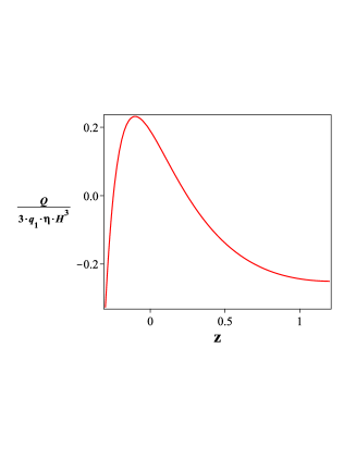
Figure 1: The picture shows the double sign change that $Q\left(q\right)$ exhibits through the evolution. We observe a one change in the past and the other in the future. Here $q_{1}=3.36$, $\overline{z}=0.54$, $\alpha/\eta=0.6$ and $\beta/\eta=0.1$. So, we have today energy transference from the bulk to the spacetime boundary.

From $q(z)$ to $\omega(z)$, the quotient $\alpha/\eta$ and the $\eta$-value. By replacing (16) into (4) we obtain

$$\omega(z)=\frac{2\eta q_{1}}{3}\left[\frac{z-\overline{z}}{\left(\alpha-3\beta/2\right)\left(1+z\right)^{2}-\beta q_{1}\left(z-\overline{z}\right)}\right],$$

and from here we can have a feeling of the $\eta$-value

$$\eta=-\frac{3\omega\left(0\right)}{2q_{1}\overline{z}}\left(\alpha-\frac{3\beta}{2}+\beta q_{1}\overline{z}\right),$$

given that we know $\omega(0)$, $q_{1}$, $\overline{z}$, $\alpha$ and $\beta$. For instance, if we use $q_{1}=3.36$, $\overline{z}=0.54$ and the set of values for $\omega(0)$, $\alpha$ and $\beta$ given in Lepe2010 , we can verify that $\alpha/\eta<1$ and $0<\eta<1$ (ghost graviton), and so we verify also that $Q(0)>0$.

IV $Q(z)$ and $\omega(z)$ - parametrization

We come back to (1) and we solve by incorporating (3) and by doing $\beta=0$ , for simplicity. First, we consider $\omega=const$. In this case, the solution of (1) is

$$H\left(z\right)=H_{0}\left(1+z\right)^{3\left(1+\left(\alpha/\eta\right)\omega\right)/2},$$ (24)

where we have used the redshift parameter $z$ defined by $1+z=a_{0}/a$, where $a$ is the cosmic scale factor. By using (3) in (2) we obtain

$$\frac{Q}{9\alpha H^{3}}\left(z\right)=-\omega\left(1-\frac{\alpha}{\eta}\right),$$ (25)

where $H(z)$ is given in (24). Using (4) we can write, for instance,

$$q(0)=\frac{1}{2}\left[1+3\frac{\alpha}{\eta}\omega(0)\right],$$ (26)

where $\omega(0)<0$ and $q(0)<0$ are both observational parameters, such that we are able to write the following constraint for $\alpha/\eta$

$$\frac{\alpha}{\eta}>\frac{1}{3}\left|\omega\left(0\right)\right|\sim\frac{1}{3},$$ (27)

then $\eta>0$, as has been seen before. Therefore, according to (25) and (27) we obtain

$$\frac{Q}{9\alpha H^{3}}\left(0\right)=-\omega(0)\left(1-\frac{\alpha}{\eta}\right)=\left|\omega(0)\right|\left(1-\frac{\alpha}{\eta}\right)$$

$$\Longrightarrow Q(0)>0\;\;if\;\;\frac{\alpha}{\eta}<1,$$ (28)

and then, if we want $Q(0)>0$, we can establish the following constraint for the ratio $\alpha/\eta$ : $1/3<\alpha/\eta<1$.

If later on we have $\omega<0$ and we consider (24), we have

$$1-\left(\alpha/\eta\right)\left|\omega\right|=$$

$$\left\{\begin{array}[]{c}>0\longleftrightarrow\left|\omega\right|<(\frac{\alpha}{\eta})^{-1}\Longrightarrow H(z\rightarrow-1)\rightarrow 0:qe,\\ <0\longleftrightarrow\left|\omega\right|>(\frac{\alpha}{\eta})^{-1}\Longrightarrow H(z\rightarrow-1)\rightarrow\infty:ph,\end{array}\right.$$ (29)

and if $\alpha/\eta=\left|\omega\right|^{-1}<1$ ($\left|\omega\right|>1$, like phantom), we have $H(z)=const$, i.e., a de Sitter phase and not necessarily $\omega=-1$.

We inspect now (24) and (25) by considering different stages of the evolution (each characterized by $\omega=const$). According to (IV) and independently of $\eta$, for $\omega=0$ (dust as the dominant component) we have $Q=0$. For $\omega>0$ we will always have $sgnQ(z)=-sgn(1-\alpha/\eta)<0$ and if $\omega<0$, $sgnQ(z)=sgn(1-\alpha/\eta)>0$, if $\alpha/\eta<1$. And yet there nothing that we can visualize yet about the possibility of an explicit sign change of $Q(z)$ through the evolution if $\omega=const$. We study this possibility by using the usual Chevallier-Polarski-Linder parametrization given by $\omega(z)=\omega(0)+{\omega}^{\prime}(0)z(1+z)^{-1}$ Chevallier2001 and as we can see in the literature Jassal2005 , the sign of ${\omega}^{\prime}(0)=$ $d\omega/dz$ at $z=0$, is model-dependent according to the fit-values from the observational data. In our analysis, however, we discuss both options for the sign of ${\omega}^{\prime}(0)$. Therefore, using (1) and (3), it is straightforward to obtain the following solution for the Hubble parameter

$$H(z)=H_{0}\left(1+z\right)^{\left(3/2\right)\left[1+\left(\alpha/\eta\right)\left(\omega\left(0\right)+{\omega}^{\prime}\left(0\right)\right)\right]}$$

$$\times\exp\left(-\frac{3}{2}\frac{\alpha}{\eta}{\omega}^{\prime}\left(0\right)\frac{z}{1+z}\right),$$ (30)

and in this case we obtain for $Q(z)$ the expression

$$\frac{Q\left(z\right)}{9\alpha H_{0}^{3}}=-\omega(0)\left(1+z\right)^{\left(9/2\right)\left[1+\left(\alpha/\eta\right)\left({\omega}^{\prime}(0)+{\omega}(0)\right)\right]}$$

$$\times\left[1-\frac{\alpha}{\eta}+\frac{{\omega}^{\prime}(0)}{\omega(0)}\frac{z}{1+z}\right]\exp\left(-\frac{9}{2}\frac{\alpha}{\eta}{\omega}^{\prime}(0)\frac{z}{1+z}\right),$$ (31)

and

$$\frac{Q(z\rightarrow\infty)}{9\alpha H_{0}^{3}}\longrightarrow-\omega(0)\left(1+z\right)^{\left(9/2\right)\left[1+\left(\alpha/\eta\right)\left(\omega(0)+{\omega}^{\prime}(0)\right)\right]}$$

$$\times\left[1-\frac{\alpha}{\eta}+\frac{{\omega}^{\prime}(0)}{\omega(0)}\right]\exp\left(-\frac{9}{2}\frac{\alpha}{\eta}{\omega}^{\prime}(0)\right),$$ (32)

where $sgn\left[Q(z\rightarrow\infty)\right]=sgn\left[1-\alpha/\eta+{\omega}^{\prime}\left(0\right)/\omega\left(0\right)\right]$. If $Q\left(z\rightarrow\infty\right)$ has to be finite and positive at early times (reasonable consideration, see [1]), we must have $1+\left(\alpha/\eta\right)\left(\omega\left(0\right)+{\omega}^{\prime}\left(0\right)\right)<0$, i.e., ${\omega}^{\prime}\left(0\right)<0$, given that $\left|\omega\left(0\right)\right|\sim 1$ and $1-\alpha/\eta+{\omega}^{\prime}\left(0\right)/\omega\left(0\right)>0$.

Now, we inspect now the sign change of $Q\left(z\right)$. By using (IV), we perform

$$Q\left(z_{0}\right)=0\longleftrightarrow z_{0}=-\left(1+\frac{{\omega}^{\prime}\left(0\right)/\omega\left(0\right)}{1-\alpha/\eta}\right)^{-1},$$ (33)

and then $-1<z_{0}<0$ if $\alpha/\eta<1$ and ${\omega}^{\prime}\left(0\right)<0$, given that $\omega\left(0\right)<0$. So, $Q\left(z\right)$ will undergo a sign change in the future. This fact is consistent with the display of Figure 1. For completeness, by using (33) we write (IV) in the form

$$\frac{Q\left(z\right)}{9\alpha H_{0}^{3}}=-\omega\left(0\right)\left(1-\frac{\alpha}{\eta}\right)\left(1+z\right)^{\left(9/2\right)\left[1+\left(\alpha/\eta\right)\left(\omega\left(0\right)+{\omega}^{\prime}\left(0\right)\right)\right]}$$

$$\times\left[1-\left(\frac{1+z_{0}}{1+z}\right)\frac{z}{z_{0}}\right]e^{-\frac{9}{2}\frac{\alpha}{\eta}{\omega}^{\prime}\left(0\right)\frac{z}{1+z}},$$ (34)

and so we can better visualize the sign change of $Q\left(z\right)$. We note that in (34), the potency of $\left(1+z\right)^{9/2}$ can be written in the form

$$1-\left(\alpha/\eta\right)\left|\omega\left(0\right)\right|\left[1+\left|{\omega}^{\prime}\left(0\right)/\omega\left(0\right)\right|\right],$$ (35)

and, independently of $sgn(1-(\alpha/\eta)|\omega(0)|(1+|{\omega}^{\prime}(0)/\omega(0)|))$, the exponential behavior is what decides the treated limits.

We consider now the limit $Q\left(z\longrightarrow-1\right)$. In this case, according to (IV) we have

$$\frac{Q\left(z\longrightarrow-1\right)}{9\alpha H_{0}^{3}}\longrightarrow{\omega}^{\prime}\left(0\right)$$

$$\times\lim_{z\longrightarrow-1}\left(1+z\right)^{\left(9/2\right)\left[7/9+\left(\alpha/\eta\right)\left(\omega\left(0\right)+{\omega}^{\prime}\left(0\right)\right)\right]}$$

$$\times\exp\left(\frac{9}{2}\frac{\alpha}{\eta}{\omega}^{\prime}\left(0\right)\frac{1}{1+z}\right),$$ (36)

and if ${\omega}^{\prime}\left(0\right)<0$, then $Q\left(z\longrightarrow-1\right)\rightarrow-0$ and, according to (IV), $H$ $\left(z\rightarrow-1\right)\rightarrow 0$. Therefore, there is energy transference from the bulk to the boundary as just was seen in Section III.

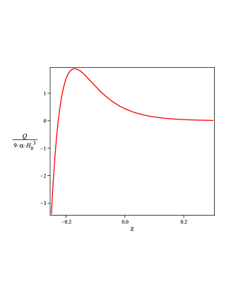
Figure 2: The picture shows only a sign change of $Q\left(z\right)$ (in the future) due to the fact that we considered $\beta=0$. If we compare with Figure 1, we note clearly the role of $\beta\neq 0$. Here $\alpha/\eta=0.6$, $\omega\left(0\right)=-1.1$ and $\acute{\omega}\left(0\right)=-1.5$

Finally, we have to ask what happens if we consider ${\omega}^{\prime}\left(0\right)>0$? This is an open issue to discuss (do not forget that $sgn\left[{\omega}^{\prime}\left(0\right)\right]$ is model-dependent, see Jassal2005 ). For the purposes of this discussion, for instance, we can maintain the idea of $Q\left(0\right)>0$ and thus discuss the consistency with the previous analysis done in this Section. This discussion will not be undertaken here.

V $\rho=3\left(\alpha{H}^{2}+\beta\dot{H}\right)$ on early Hořava-Lifshitz cosmology

We consider now the following equations

$$3\eta H^{2}=\rho-\gamma\frac{k^{3}}{a^{6}},$$ (37)

and

$$\eta\left(2\dot{H}+3H^{2}\right)=-\omega\rho+\gamma\frac{k^{3}}{a^{6}},$$ (38)

where $k=0,\pm 1$ (curvature index) and $\gamma$ is a constant. In Hořava-Lifshitz cosmology, the scheme (35-36) is generated by considering only terms in which $a^{-6\text{ }}$ is the dominant one Mukohyama2010 . A term like $\gamma k^{3}a^{-6}$ is reminiscent of stiff matter (in GR: $p=\rho\rightarrow\rho\sim a^{-6}$) and its presence (stiff matter) at early stages of the evolution may have played an important role under the scope of a holographic approach to cosmology BanksFischler04 . In Bambi2014 a Friedmann equation is derived from a four-fermion interaction, and where a $a^{-6}$-like term appears naturally which is used there, in addition to a dust term $a^{-3}$, to avoid possible cosmic singularities. From (37, 38) we can obtain

$$2\eta\left(\dot{H}+3H^{2}\right)=\left(1-\omega\right)\rho,$$ (39)

and after replacing the given cut-off in the last equation, we have

$$d\ln H\left(z\right)=\left(\frac{2-\left(\alpha/\eta\right)\left(1-\omega\right)}{2-\left(3\beta/\eta\right)\left(1-\omega\right)}\right)d\ln\left(1+z\right)^{3},$$ (40)

and if $\omega=1$ or $\eta\longrightarrow\infty$, or also $\alpha=3\beta$ (although this equality is not required by observational fits Lepe2010 ; Arevalo2014 ), the Hubble parameter and the cosmic scale factor are, respectively,

$$H\left(z\right)=H_{0}\left(1+z\right)^{3}\longrightarrow$$

$$a\left(t\right)=a_{0}\left[1+3H_{0}\left(t-t_{0}\right)\right]^{1/3}\Longrightarrow\ddot{a}\left(t\right)<0,$$ (41)

i.e., the same solution as found in GR ($3H^{2}=\rho$ and $\dot{\rho}+3H\left(1+\omega\right)\rho=0$ with $\omega=1$); nevertheless, in the present case we have non-null curvature (see (37, 38)). If we consider now $\omega=-1$, we have

$$H\left(z\right)=H_{0}\left(1+z\right)^{3\Delta}\text{ \ \ }$$

and    

$$\Delta=\left(1-\alpha/\eta\right)/\left(1-3\beta/\eta\right),$$ (42)

and the cosmic scale factor and the acceleration are given, respectively, by

$$a\left(t\right)=a_{0}\left[1+3\Delta H_{0}\left(t-t_{0}\right)\right]^{1/3\Delta},$$ (43)

(a power-law solution) and

$$\ddot{a}\left(t\right)=a_{0}H_{0}^{2}\left(1-3\Delta\right)\left[1+3\Delta H_{0}\left(t-t_{0}\right)\right]^{\left(1/3\Delta\right)-2}.$$ (44)

Now, if $1/6<\Delta<1/3$ the acceleration given in (44) is positive and decreases in time although $\omega=-1$. But, at early times we expect to have something like $H\sim H_{0}$ (old inflation-like), i. e., according to (42) $\alpha/\eta\sim 1\Longrightarrow\omega\sim-1$ and in this case $a\left(t\right)\sim\exp\left(H_{0}t\right)$. Hence, the ratio $\alpha/\eta$ is very important here. In particular, if we put $\beta=0$ ($\Delta=1-\alpha/\eta>0\longleftrightarrow\alpha/\eta<1$) we write

$$a\left(t\right)=a_{0}\left[1+3\left(1-\frac{\alpha}{\eta}\right)H_{0}\left(t-t_{0}\right)\right]^{1/3\left(1-\alpha/\eta\right)},$$

$$\Longrightarrow H(t)=H_{0}\left[1+3\left(1-\frac{\alpha}{\eta}\right)H_{0}\left(t-t_{0}\right)\right]^{-1}$$ (45)

and the acceleration is

$$\ddot{a}\left(t\right)=a_{0}H_{0}^{2}\left[1-3\left(1-\frac{\alpha}{\eta}\right)\right]$$

$$\times\left[1+3\left(1-\frac{\alpha}{\eta}\right)H_{0}\left(t-t_{0}\right)\right]^{-2\left(\alpha/\eta-5/6\right)/\left(\alpha/\eta-1\right)},$$ (46)

and by considering the inequality $2/3<\alpha/\eta<5/6$ (and $Q\left(z=0\right)>0$, see Sections II, III and IV) the acceleration given in (V) is , as was stipulated, positive and decreases with time, although $\omega\approx-1$.

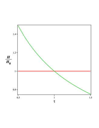
Figure 3: The Hubble parameter given in (V) compared with $H=const$(usual de Sitter phase). Here $\alpha/\eta=0.78$.

A similar pattern to that shown in Figure 3 is discussed in DiMarco2006 under the idea of ”graceful” old inflation. There, the authors have shown that cite: a false vacuum can successfully decay to a true vacuum, producing inflation, … ,since exponential inflation is slowed down to power-law Inflation. Thus, the present scheme built under the holographic philosophy of HL cosmology could be considered a new antecedent giving an alternative to previous studies done.

Early phantom phase. We consider $\Delta<0$ ($3\beta<\eta<\alpha$ or $\alpha<\eta<3\beta$) (see [3,5] for $\alpha$ and $\beta$ values). In this case we have for the Hubble parameter the solution $H\left(t\right)=\left(H_{0}/3\left|\Delta\right|\right)\left(t_{s}-t\right)^{-1}$, where $t_{s}=t_{0}+\left(1/3\left|\Delta\right|\right)H_{0}^{-1}$ and for the scale factor we obtain $a\left(t\right)=a_{0}\left(3\left|\Delta\right|H_{0}\right)^{-1/3\left|\Delta\right|}\left(t_{s}-t\right)^{-1/3\left|\Delta\right|}$. If we put $\beta=0$ and $\alpha/\eta>1$ ($\Delta<0$), the role of $\alpha/\eta$ in the raised phantom scheme becomes more evident. Do not forget that we have with $\omega=-1$ from (42) to (V), meaning that we have an ”early” phantom scheme without requiring $\omega<-1$. Nevertheless, at early times we do not have a singularity according to the observational data and therefore, we discard this early behavior and then we have again a strong argument for claiming that $0<\alpha/\eta<1$ (and so, positive $\eta$).

According with (44), $\ddot{a}\left(t\right)>0$ and not a phantom ($\Delta>0$) $\Longrightarrow 0<\left(1-\alpha/\eta\right)/\left(1-3\beta/\eta\right)<1/3$, we obtain

$$0<\left(\eta-\alpha\right)/\left(\eta-3\beta\right)<1/3\Longrightarrow$$

$$\alpha/\eta<1\text{ \ \ }and\text{ \ }\eta>3\beta,$$ (47)

or

$$0<\left(\alpha-\eta\right)/\left(3\beta-\eta\right)<1/3\Longrightarrow$$

$$\alpha/\eta>1\text{ \ \ }and\text{ \ }\eta<3\beta,$$ (48)

and in this last case we can have both options $\eta\gtrless 0$. If $\eta<0$, we write

$$0<\left(\left|\eta\right|+\alpha\right)/\left(\left|\eta\right|+3\beta\right)<1/3\Longrightarrow\frac{2}{3}\left|\eta\right|+\alpha<\beta,$$ (49)

and this option is discarded given that $\alpha>\beta$ Lepe2010 ; BingWang2007 . We note that, in the present situation, the limit $\eta\rightarrow\infty$ does not operate. So, $\alpha/\eta<1$ and we have no phantom and we agree with the discussions performed before.

Finally, by using the $q$-parameter and the given holographic cut-off, from (26) we can write

$$1+q=3\left(\frac{2-\left(\alpha/\eta\right)\left(1-\omega\right)}{2-3\left(\beta/\eta\right)\left(1-\omega\right)}\right),$$ (50)

and we can notice that $\omega=1$ or $\eta\longrightarrow\infty$, both leading to $q=2$ (usual stiff matter behavior as in GR). If we are thinking in ”old inflation”, i.e., $\omega\sim-1$, we have

$$1+q\sim 3\left(\frac{1-\alpha/\eta}{1-3\beta/\eta}\right),$$ (51)

and only in the case $\alpha/\eta\sim 1$ we recover $q\sim-1$ (as GR).

VI Thermal aspects

Some studies have considered the possibility of energy interchange between the bulk and the spacetime boundary LepePe a2014 . If we are think about thermal equilibrium between the bulk and the boundary, the answer is not reflecting our results. There is non-equilibrium given that there are two changes in the direction of the energy interchange: one in the past ($z>0$ ) and other in the future ($-1<z<0$) if $\beta\neq 0$ or only one change (in the future) if $\beta=0$. What is the sign of $Q\left(0\right)$? The answer is fully dependent on $\eta$, $sgn\left(\eta\right)$ and the values of $\alpha$ and $\beta$. And we have $Q\left(0\right)>0$ in accordance with the obtained and well justified constraint $0<\alpha/\eta<1.$ On the other hand, if we consider $\eta<0$ from heading and by using (6), we have

$$\frac{Q}{6H^{3}}=\left|\eta\right|\left(1+\frac{\alpha}{\left|\eta\right|}\right)\left(q-\frac{1}{2}\right),$$ (52)

and given that $q\left(0\right)<0$, then $Q\left(0\right)<0$. But, if we considerer(26) we obtain

$$q\left(0\right)=\frac{1}{2}\left(1+3\alpha\left|\frac{\omega\left(0\right)}{\eta}\right|\right)>0,$$ (53)

and there is an inconsistency with the observational data: $q\left(0\right)<0$. Therefore, we apologize that $\eta>0$ is consistent with the current observational data, and hence we emphasize that $q\left(0\right)<0$ is a crucial antecedent to justify what we have developed here.

VII Conclusions

We have shown the existence of sign changes, through the evolution, of the amount of non-conservation energy $Q\left(z\right)$ present in the framework of the Hořava-Lifshitz cosmology as a consequence of the philosophy of a holographic scheme assigned to the energy-matter content in the theory. We have analyzed the late limit and the early limit (where a reminiscent stiff like-matter term is one dominant), and we do not observe phantom phases, in any event, if $\alpha/\eta<1$. At early times, we have found a power-law solution for the cosmic scale factor, although $\omega=-1$, and this fact may be considered a new antecedent to consider if we think about in old inflation. Is it possible to respond to this concern, the old inflation problem, within the framework of HL-cosmology under a holographic scope? We leave this concern for now.

Additionally, $\eta$ has been relatively well confined to the range $0<\eta<1$ according to the used observational setting for $\alpha$, $\beta$ and $\omega\left(0\right)$. And so, we can say we have a ghost scalar graviton in the present framework.

Finally, we live out the thermodynamic equilibrium and we are cooling down ($Q\left(0\right)>0$) according to what is shown here (Figures 1 and 2).

References

- (1) S. Mukohyama, Class. Quant. Grav. 27 (2010) 223101; A. Emir Gumrukcuoglu and S. Mukohyama, Phys. Rev. D 83 (2011) 124033; S. Lepe and J. Saavedra, Astrophys. Space Sci. 350 (2014) 839-843.
- (2) T. Kobayashi, Y. Urakawa and M. Yamaguchi, JCAP 0911 (2009) 015, arXiv:0908.1005.
- (3) S. Mukohyama, Phys. Rev. D 80 (2009) 064005; A. Wang and R. Maartens, Phys. Rev. D 81, 024009 (2010).
- (4) Xiao-Dong et al, JCAP 1312 (2013) 001.
- (5) L. N. Granda and A. Oliveros, Phys. Lett. B 669 (2008) 275-277.
- (6) S. Lepe and F. Peña, Eur. Phys. J. C 69 (2010) 575-579. Here and ; Yutin Wang and Lixin Xu, Phys. Rev. D 81 (2010) 083523. Here and ; M. Li et al, JCAP 1309 (2013) 021. Here , Planck data.
- (7) Bing Wang et al, Nucl. Phys. B 778 (2007) 69-84; Andrè A. Costa et al, Phys. Rev. D 89 (2014) 103531.
- (8) F. Arévalo et al, Astrophys. Space Sci. 352 (2014) 899-907. Here and .
- (9) S. Nojiri, S. D. Odintsov and S. Tsujikawa, Phys. Rev. D71 (2005) 063004.
- (10) A. Emir Gumrukcuoglu and Shinji Mukohyama, Phys. Rev. D83 (2011) 124033.
- (11) Y. Gong and A. Wang, Phys. Rev. D 75 (2007) 043520.
- (12) J. Magaña et al, arXiv:1407.1632 [astro-ph.CO].
- (13) M. Chevallier and D. Polarski, Int. J. Mod. Phys. D 10, 213 (2001) & E. V. Linder, Phys. Rev. Lett. 90, 091301 (2003).
- (14) H. K. Jassal et al, Mon. Not. Roy. Astron. Soc. 356, L11 (2005); Y. Gong and A. Wang, Phys. Rev. D 75 (2007) 043520; R. de Putter and E. V. Linder, JCAP 0810 (2008) 042; E. V. Linder, Phys. Rev. D 84 (2011) 123529; Gong-Bo Zhao et al, Phys. Rev. D 85 (2012) 123546; J. Alberto Vásquez et al, JCAP 1209 (2012) 020; Dhiraj Kumar Hazra et al, arXiv:1310.6161 [astro-ph.CO] (Planck data).
- (15) T. Banks and W. Fischler, hep-th/0412097; T. Banks, W. Fischler and L. Mannelli, Phys. Rev. D 71 (2005) 123514.
- (16) C. Bambi et al, Phys. Lett. B 734 (2014) 27-30.
- (17) F. Di Marco and A. Notari, Phys. Rev. D 73 (2006) 063514.
- (18) S. Lepe and F. Peña, Astrophys. Space Sci. 350 (2014) 401-406.