Perturbation Theory for Propagating Magnetic Droplet Solitons

Abstract

Droplet solitons are a strongly nonlinear, inherently dynamic structure in the magnetization of ferromagnets, balancing dispersion (exchange energy) with focusing nonlinearity (strong perpendicular anisotropy). Large droplet solitons have the approximate form of a circular domain wall sustained by precession and, in contrast to single magnetic vortices, are predicted to propagate in an extended, homogeneous magnetic medium. In this work, multiscale perturbation theory is utilized to develop an analytical framework for investigating the impact of additional physical effects on the behavior of a propagating droplet. After first developing soliton perturbation theory in the general context of Hamiltonian systems, a number of physical phenomena of current interest are investigated. These include droplet-droplet and droplet-boundary interactions, spatial magnetic field inhomogeneities, spin transfer torque induced forcing in a nanocontact device, and damping. Their combined effects demonstrate the fundamental mechanisms for a previously observed droplet drift instability and under what conditions a slowly propagating droplet can be supported by the nanocontact, important considerations for applications. This framework emphasizes the particle-like dynamics of the droplet, providing analytically tractable and practical predictions for modern experimental configurations.

1 Introduction

The ability to excite, probe, and control magnetic media at the nanometer scale has enabled new applications in spintronics and magnonics as well as the exploration of new physics. Of particular, recent interest is the generation of coherent structures within the magnetization, a vector field describing the magnetic dipole moments of a magnetic material. Coherent structures observed experimentally include those with nontrivial topology such as magnetic vortices Uhlíř et al. (2013); Pulecio et al. (2014) and skyrmions Nagaosa and Tokura (2013); Fert et al. (2013); Yu et al. (2014) as well as nontopological droplet solitons Mohseni et al. (2013, 2014); Chung et al. (2014); Macià et al. (2014). The magnetic droplet soliton (droplet hereafter) is a coherently precessing, nanometer-scale localized wave structure exhibiting strongly nonlinear effects Kosevich et al. (1990). Its first observation Mohseni et al. (2013) was enabled by a nano-contact spin-torque oscillator (NC-STO) device, which provides the necessary forcing to oppose magnetic damping, hence has been termed a dissipative droplet soliton Hoefer et al. (2010).

The droplet is theoretically understood as a solution of a conservative Landau-Lifshitz partial differential equation modeling spatio-temporal dynamics in an ultra thin, two-dimensional magnetic film with uniaxial, perpendicular anisotropy. When the stationary droplet’s precessional frequency is close to the local, magnetic field induced (Zeeman) frequency, it resembles a circular domain wall of large radius, almost reversed at its core. These large droplets can propagate, coinciding with a superimposed wave structure to the otherwise spatially homogeneous phase. An example is shown in Fig. 1.

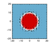
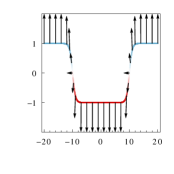
Figure 1: (a) Contour (color is $m_{z}$) and vector field, $(m_{x},m_{y})$, plot of an approximate, propagating magnetic droplet, described in Sec. 3, moving to the right with speed $V=0.02$ and precessing with frequency $\omega=0.1$. (b) The magnetization evaluated on the line $y=0$ and superimposed upon the $m_{z}$ profile. There is no phase winding across this nontopological structure.

There are a rich variety of physical mechanisms that can change the orientation of the local dipole moment in a ferromagnet and hence influence the particle-like behavior of a droplet. An example already mentioned is that of the NC-STO and damping. This motivated us to develop a droplet soliton perturbation theory that allows for the analysis of droplet dynamics in the presence of a large number of physical perturbations Bookman and Hoefer (2013). This theory describes soliton dynamics via a finite dimensional dynamical system representing the adiabatic evolution of the droplet’s four parameters (center, precessional frequency, and phase) resulting from perturbations.

While the theory provided fundamental explanations of droplet physics, it was limited to almost stationary droplets, i.e., droplets of negligible momentum, which manifested as a constraint equation on the dynamics. Furthermore, important physical effects such as droplet acceleration due to a magnetic field gradient Kosevich et al. (1998); Babich and Kosevich (2001); Hoefer et al. (2012) and droplet interactions Piette and Zakrzewski (1998); Maiden et al. (2014) were excluded from the theory.

Soliton perturbation theory has been successfully used to describe dynamics in many physical systems Kivshar and Malomed (1989); Sanchez and R. (1998), notably solitons in Nonlinear Schrödinger (NLS) type equations modeling, for example, optical fibers Yang (2010) and Bose-Einstein condensates Kevrekidis et al. (2008). The central idea is to project the perturbed PDE dynamics onto the unperturbed soliton solution manifold, allowing for adiabatic evolution of the soliton’s parameters. The resulting modulation equations can be obtained in different ways, of which multiple scales perturbation theory Keener and McLaughlin (1977) or perturbed conservation laws Kivshar and Malomed (1989) are perhaps the most common. Both approaches have been shown to be equivalent in some specific applications, see, e.g., Ablowitz et al. (2009), but the conservation law approach is powerful in its simplicity. However, it can be unclear which balance laws to use, especially when higher order information is sought. The governing Landau-Lifshitz equation for magnetization dynamics is a strongly nonlinear, vectorial generalization of the NLS equation that lacks Galilean invariance. There exist two-dimensional moving droplet solutions Piette and Zakrzewski (1998); Hoefer and Sommacal (2012) described by six independent parameters. As such, droplet perturbation theory is significantly more complex than its NLS soliton counterpart, so a structured approach is desirable.

The earliest, most general formulation of soliton perturbation theory we have found in the literature is given in Keener and McLaughlin (1977), where multiple scales perturbation theory and the Green’s function for the linearized operator are utilized. An alternative, rigorous approach was developed for the modulational stability of solitons in NLS equations in Weinstein (1985) based on multiple scales and the generalized nullspace of the linearized operator. Motivated by the challenges associated with magnetic droplet soliton perturbation theory, we revisit the general approach for perturbed Hamiltonian systems, utilizing multiple scales and the generalized nullspace formulation. In Section 2, we provide necessary conditions and expressions for the resulting modulation equations. Our approach preserves much of the generality of the Green’s function approach with the comparative accessibility of Weinstein’s approach to NLS. Additionally, we demonstrate that these methods do generalize to soliton perturbation in higher dimension, beyond (1+1)D, and how they can be used to determine the evolution of large numbers of parameters for a single soliton.

Two-dimensional moving droplet solutions have been computed Piette and Zakrzewski (1998); Hoefer and Sommacal (2012) and studied asymptotically in the weakly nonlinear regime Ivanov et al. (2001). They can be accelerated and controlled by an inhomogeneous, external magnetic field Hoefer et al. (2012) and exhibit novel interaction properties Maiden et al. (2014). Droplets can also experience a drift instability in NC-STOs, whose origin is not well-understood Hoefer et al. (2010). Because droplets are relatively new physical features of nanomagnetic systems, they hold potential for applications such as spintronic information storage and transfer or probing material properties. Moreover, their fundamental physics are not well understood. A more general theory to describe the motion of droplets in realistic physical systems is desirable.

Toward this end, we here present an analytical framework for investigating the impact of a large class of physical effects on a six parameter propagating droplet soliton. In Section 3, we derive an approximate solution for the propagating droplet in the close to Zeeman frequency (large mass) and small velocity (order one momentum) regime, which greatly reduces the complexity of the asymptotic theory developed. This allows for explicit analytical results, a powerful feature of soliton perturbation theory considering the droplet’s strongly nonlinear qualities. The main result of this paper, the modulation equations, is presented in Section 4, utilizing the general soliton perturbation theory formulation from Section 2. The versatility of this framework is subsequently discussed in Sections 5 and 6 through an investigation of a series of perturbations of current physical interest. In particular, we analytically demonstrate a mechanism leading to the NC-STO droplet drift instability and why a droplet can be attracted or repelled by a ferromagnetic boundary.

The model under study here is the perturbed Landau-Lifshitz equation for the magnetization, $\mathbf{m}=[m_{x},m_{y},m_{x}]$, of a two-dimensional ferromagnetic film in nondimensional form

$$\begin{split}\frac{\partial\mathbf{m}}{\partial t}&=-\mathbf{m}\times\mathbf{h}_{\rm eff}+\epsilon\mathbf{p},\quad\mathbf{m}:\mathbb{R}^{2}\times(0,\infty)\to\mathbb{S}^{2},\\ \mathbf{h}_{\rm eff}&=\nabla^{2}\mathbf{m}+\left(h_{0}+m_{z}\right)\mathbf{\hat{z}},\quad\lim_{|\mathbf{x}|\to\infty}\mathbf{m}=\mathbf{\hat{z}},\end{split}$$ (1)

where $\mathbf{p}$ is a perturbation that preserves the magnetization’s length ($\mathbf{p}\cdot\mathbf{m}\equiv 0$) and $0<\epsilon\ll 1$ is a small parameter encoding the strength of the perturbation. The perturbation can depend explicitly on time so long as the variation is slow. That is, the perturbation depends only on the slow temporal coordinate $T=\epsilon t$. The perpendicular, external magnetic field $h_{0}\mathbf{\hat{z}}=h_{0}(\mathbf{X},T)\mathbf{\hat{z}}$ can be large and slowly varying in space ($\mathbf{X}=\epsilon\mathbf{x}$) and time. Further generalizations to rapidly varying perturbations are possible. A necessary requirement for the existence of droplet solitons is strong perpendicular anisotropy, encoded in the orientation of the $m_{z}\mathbf{z}$ term in the effective field $\mathbf{h}_{\rm eff}$. See Bookman and Hoefer (2013) for the derivation and nondimensionalization of this model.

2 Adiabatic Dynamics for Hamiltonian Systems

The main aim of this paper is to determine the evolution of parameters of the droplet soliton in response to a fairly general class of perturbations. The equations determining the time-evolution of parameters will be referred to as modulation equations. Before performing that analysis directly, we first consider the more general context of perturbed Hamiltonian systems. Note that the Landau-Lifshitz equation is a Hamiltonian system, with canonically conjugate variables $\cos(\Theta)$, $\Phi$. That is, the Landau-Lifshitz system may be written as $\frac{\partial\cos\Theta}{\partial t}=\frac{\delta\mathcal{E}}{\delta\Phi}$ and $\frac{\partial\Phi}{\partial t}=-\frac{\delta\mathcal{E}}{\delta\cos\Theta}$, where the right hand sides are expressed in terms of variational derivatives of the energy $\mathcal{E}$, defined later in eq. (17). In such systems, it is more convenient to execute perturbation theory in the Hamiltonian variables. It is also possible to write down modulation equations for solitons with parameters related in a particular way. This statement will be made more precise later in this section.

The basic procedure is to allow the parameters to vary on a time scale proportional to the strength of the perturbation, $\epsilon$. By allowing the parameters to vary in this way, additional degrees of freedom are introduced which can be used to resolve the difficulties arising from singular perturbations. Expanding about the soliton solution in an asymptotic series, one obtains a linear problem at order $\epsilon$. In general, this linear equation will not admit solutions bounded in time. However, as utilized in Weinstein (1985), a solvability condition exists whereby bounded solutions are assured, guaranteeing that the linear problem at order $\epsilon$ does not break the asymptotic ordering. Imposing these conditions leads to the modulation equations. This procedure is equivalent to projecting the solution of the perturbed model onto the family of solitons. While one might wish to then solve the linear equation at order $\epsilon$ to obtain a further correction, we will not do that in this work. As will be demonstrated by the examples in Sec. 5, quite satisfactory predictions can be made considering only the leading order dynamics.

A Hamiltonian system requires a real inner product space, $X$; a nonlinear functional, $H:X\rightarrow\mathbb{R}$; and a skew adjoint operator $J:X\rightarrow X$. We will use the notation $\langle\cdot,\cdot\rangle$ for the inner product on $X$. The standard form for a Hamiltonian system is

$$\frac{\partial z}{\partial t}=J\nabla H(z)$$ (2)

where $z\in X$ is referred to as the state variable. We refer to $H$ as the Hamiltonian, which is often assigned the physical meaning of energy since it is automatically a conserved quantity of such a system. In this context, by $\nabla H$ we mean the first variation of this nonlinear functional and by $\Delta H$ we mean the second variation (both taken with respect to the state variable, $z$). We consider here Hamiltonians which depend explicitly upon additional parameters, $\mathbf{q}\in\mathbb{R}^{m}$ ($m$ is the number of such parameters). Such parameters may arise due to a change of coordinates, such as to a comoving reference frame. For the examples which arise in this work, the parameters $\mathbf{q}$ arise from just such a transformation, so we will typically refer to these parameters as “frequencies".

We assume here that (2) admits a solitary wave solution, $u$.

$$0=J\nabla H(u,\mathbf{q}).$$ (3)

If $H$ depends on $\mathbf{q}$, naturally $u$ will depend on $\mathbf{q}$ as well. Typically, the parameters $\mathbf{q}$ do not provide a full parameterization of the solitary wave manifold due to underlying symmetries in the equation such as translation invariance. Accordingly, we will allow $u$ to depend on a separate set of parameters $\mathbf{r}\in\mathbb{R}^{s}$ ($s$ is the number of such parameters). For reasons that will become clear in later examples we refer to these parameters as “phases”. Therefore, the solitary wave can be written $u=u(\mathbf{x};\mathbf{q},\mathbf{r})$. Often times, the Hamiltonian system (2) admitting solitary wave solutions (3) is idealized, neglecting important physical effects. While some perturbations may give rise to a different Hamiltonian system, in general such effects do not need to preserve the Hamiltonian structure. We will treat both cases the same by introducing a small perturbation into the equation itself. The perturbed model is

$$\frac{\partial z}{\partial t}=J\nabla H(z,\mathbf{q})+\epsilon P$$ (4)

where $0<\epsilon\ll 1$ and $P$ is a perturbation. The parameters $\mathbf{q},\mathbf{r}$ are allowed to vary on a slow time scale, $T=\epsilon t$. We restrict to perturbations which depend explicitly on time only through this slow time variable, $T$. In this case, ordinary differential equations governing the evolution of these parameters can be determined according to the following theorem.

Theorem 1.

Given the perturbed Hamiltonian system (4). If

1. The solitary wave solution, $u$, exists for the unperturbed system (4), $\epsilon=0$, and is independent of $t$.

2. $J$ is invertible.

3. $\Delta H\bigg{|}_{z=u}$ is self-adjoint for all admissible $\mathbf{q}$.

4. $\forall\;1\leq k\leq m$, $\exists\;1\leq j\leq s$ such that $\frac{\partial}{\partial q_{k}}\nabla H(z,\mathbf{q})\bigg{|}_{z=u}=-J^{-1}\frac{\partial u}{\partial r_{j}}$

then letting $\mathbf{v}=\left[\mathbf{r},\mathbf{q}\right]^{T}\in\mathbb{R}^{s+m}$, the modulation equations are

$$\begin{array}[]{rcl}\displaystyle\left(\sum_{i=1}^{s+m}\left\langle J^{-1}\frac{\partial u}{\partial v_{i}},\frac{\partial u}{\partial v_{j}}\right\rangle\frac{dv_{i}}{dT}\right)&\displaystyle=&\displaystyle\left\langle J^{-1}P,\frac{\partial u}{\partial v_{j}}\right\rangle\end{array}$$ (5)

Equation 5 is consistent with previous general results when applied to Hamiltonian systems Keener and McLaughlin (1977). The assumptions of Theorem 1 may seem restrictive at first, but these conditions are frequently met in physical systems of interest. In all systems under consideration here there does exist a solitary wave solution. These solutions generically depend on time, but for the case of a single solitary wave solution, transforming to the reference frame moving, rotating, and/or precessing with the solitary wave can eliminate this explicit dependence on time. Such a transformation will introduce parameters in $\mathbf{q}$ and alter the Hamiltonian but leaves the Hamiltonian structure intact.

The second does offer a restriction. For instance, in the Korteweg-de-Vries equation, $J$ does not admit a bounded inverse and correspondingly the modulation equations require additional considerations Ablowitz and Segur (1981). Nevertheless, formal calculations are possible and $J$ is frequently invertible for Hamiltonian systems (as it is, e.g., for NLS and the Landua-Lifshitz equation).

With appropriate restrictions on the Hamiltonian, the third assumption always holds. The self-adjoint property of the second variation essentially follows from the same calculation which proves the equality of mixed partial derivatives in finite-dimensional calculus. More care needs to be taken in the corresponding calculation on function spaces, but the Hamiltonians derived in physically relevant systems typically are well enough behaved.

The fourth assumption is restrictive and may seem obscure. However, the parameters of the soliton are often speeds or frequencies. These parameters are typically linked to initial positions or initial phase values so that $\mathbf{q}$ and $\mathbf{r}$ have the same length ($s=m$). In such cases, the dependence of the soliton on the parameters in the laboratory frame will be in the form $\mathbf{r}+t\mathbf{q}$. From this temporal dependence, the relations in Assumption (iv) follow directly.

2.1 Derivation of Equation (5)

Theorem 1 relies on the following lemma.

Lemma 1.

Let $X$ be a Hilbert space. Let $A$ be a linear operator mapping $X$ to itself. Let $f\in X$. Let $A^{\dagger}$ be the adjoint of $A$, i.e. the unique linear operator satisfying $\langle A^{\dagger}x,y\rangle=\langle x,Ay\rangle$ for all $x,y\in X$. Define $\Upsilon:[0,\infty)\rightarrow X$ as the solution of the initial value problem

$$\begin{cases}\frac{\partial\Upsilon}{\partial t}=A\Upsilon+f\\ \Upsilon(0)=\Upsilon_{0}\in X.\end{cases}$$ (6)

Let $\mu_{-1}=0$ and $A^{\dagger}\mu_{i}=\mu_{i-1}$ for $0\leq i\leq N$, where $N$ denotes the highest integer such that $(A^{\dagger})^{N}$ has nontrivial kernel. Then $\Upsilon(t)$ will not be bounded in time unless $\left\langle\mu_{i-1},\Upsilon_{0}\right\rangle+\left\langle\mu_{i},f\right\rangle=0$ for $0\leq i\leq N$.

This lemma is a minor generalization of the solvability condition proven in Weinstein (1985). There are a few key limitations which may not be clear upon first reading the statement of the lemma itself. First, $A$ and $f$ are assumed to be independent of time $t$. Second, all assumptions of smoothness of $f$ are bound up in the choice of $X$ which is problem specific. In the context of Hamiltonian systems, $X$ is given and the required smoothness of $f$ is clear. In our intended application, Eq. (6) arises from a linearization of a nonlinear problem about a given state. In this case, $A$ and $f$ are given, but not $X$. In order that Lemma 1 applies, there must exist an $X$ which makes $A$ and $f$ compatible, and it will be in that sense which $\Upsilon(t)$ remains bounded in time. From here on out, we assume sufficient smoothness in our perturbation such that a Hilbert space is naturally chosen. For the perturbations we investigate in Section 5, this is the case. Finally, the details of defining the adjoint of the unbounded operator $A$ are not considered here but can be handled in a standard manner; see, e.g., Weinstein (1985).

The proof of Theorem  1 proceeds by substituting the ansatz

$$z=u(\mathbf{r}(T),\mathbf{q}(T))+\epsilon u_{1}(\mathbf{x},t,T)+\mathcal{O}\left(\epsilon^{2}\right)$$ (7)

into (4). Expanding in powers of $\epsilon$, the first order equation becomes

$$\mathcal{O}\left(\epsilon\right):\hskip 14.22636pt\frac{\partial u_{1}}{\partial t}=J\Delta H(u,\mathbf{q})u_{1}-\frac{\partial u}{\partial\mathbf{r}}\frac{d\mathbf{r}}{dT}-\frac{\partial u}{\partial\mathbf{q}}\frac{d\mathbf{q}}{dT}+P$$ (8)

Note that Eq. (8) is of the form in Lemma 1 ($A=J\Delta H(u,\mathbf{q})$, $f=P-\frac{\partial u}{\partial\mathbf{r}}\frac{d\mathbf{r}}{dT}-\frac{\partial u}{\partial\mathbf{q}}\frac{d\mathbf{q}}{dT}$). In order that the expansion in (7) remain asymptotically ordered, it is necessary that $u_{1}(x,t,T)$ remain $\mathcal{O}\left(1\right)$ for sufficiently long times. Lemma 1 thus gives a condition that must be satisfied. It remains to characterize the generalized nullspace of $(J\Delta H(u,\mathbf{q}))^{\dagger}$. Note that since $\Delta H(u,\mathbf{q})$ is self-adjoint, $(J\Delta H(u,\mathbf{q}))^{\dagger}=-\Delta H(u,\mathbf{q})J$.

Differentiating (3) with respect to the parameter $r_{j}$ for $1\leq j\leq s$ and applying $J^{-1}$ to the result yields $\Delta H(u,\mathbf{q})\frac{\partial u}{\partial r_{j}}=0$. It follows that $J^{-1}\frac{\partial u}{\partial r_{j}}$ is in the kernel of $(J\Delta H(u,\mathbf{q}))^{\dagger}$ for all $j$. Differentiating (3) with respect to the parameter $q_{k}$ for $1\leq k\leq m$ yields

$$\Delta H(u,\mathbf{q})\frac{\partial u}{\partial q_{k}}+\frac{\partial}{\partial q_{k}}\nabla H(z,\mathbf{q})\bigg{|}_{z=u}=0.$$ (9)

Utilizing assumption (iv), we can replace the second term in (9) so that there is some $j$ with

$$\Delta H(u,\mathbf{q})J\left(J^{-1}\frac{\partial u}{\partial q_{k}}\right)=J^{-1}\frac{\partial u}{\partial r_{j}}.$$ (10)

Hence, $J^{-1}\frac{\partial u}{\partial q_{k}}\in\ker(\Delta H(u,\mathbf{q})J)^{2}$ and therefore in the generalized nullspace. These two sets of vectors do not necessarily characterize the full generalized nullspace; however, these offer a sufficient number of constraints to uniquely determine the modulation system. Requiring that $f=P-\frac{\partial u}{\partial\mathbf{r}}\frac{d\mathbf{r}}{dT}-\frac{\partial u}{\partial\mathbf{q}}\frac{d\mathbf{q}}{dT}$ be orthogonal to $J^{-1}\frac{\partial u}{\partial q_{k}}$ and $J^{-1}\frac{\partial u}{\partial r_{j}}$ yields equations (5). The modes $J^{-1}\frac{\partial u}{\partial q_{k}}$ and $J^{-1}\frac{\partial u}{\partial r_{j}}$ may not give rise to a complete characterization of the nullspace. As a result, Eqs. (5) are only a necessary but not sufficient condition to prevent secular growth.

3 Approximate Propagating Droplet

Now that we have the general formulation of the soliton modulation equations for perturbed Hamiltonian systems in eq. (5), we would like to apply them to the magnetic droplet soliton solution of eq. (1). For this, we will need to compute derivatives of the droplet with respect to its parameters as well as associated inner products. This could be performed numerically with a “database” of droplet solutions as in Hoefer et al. (2012). Here, we obtain an explicit, analytical formulation of the modulation equations in the strongly nonlinear, moving droplet regime. But before we can determine the modulation equations, we need an explicit representation of the propagating droplet itself. In this section, we derive an approximate solution to eq. (1) when $\epsilon=0$, a restriction we maintain for the remainder of this section. The solution describes a slowly moving droplet with frequency just above the Zeeman frequency. A droplet solution can be characterized by six parameters: its precession frequency $\omega$ above the Zeeman frequency $h_{0}$ in these non-dimensional units, propagation velocity $\mathbf{V}=[V_{x},V_{y}]^{T}$, initial phase $\Phi_{0}$, and the coordinates of the droplet center $\boldsymbol{\xi}=[\xi_{x},\xi_{y}]^{T}=\mathbf{V}t+\mathbf{x}_{0}$.

Approximate droplet solutions have been found in two regimes: (i) $0<1-\omega-|\mathbf{V}|^{2}/4\ll 1$, near the linear (spin-wave) band edge corresponding to propagating, weakly nonlinear droplets approximated by the NLS Townes soliton Ivanov et al. (2001) (ii) $0<\omega\ll 1$ with zero velocity corresponding to stationary, strongly nonlinear droplets approximated by a circular domain wall Kosevich et al. (1986); Ivanov and Stephanovich (1989). We will focus here on large amplitude propagating solitons where the magnetization is nearly reversed because experiments operate in this regime. Note, however, that the weakly nonlinear regime could also be studied. The defining equation for the droplet can be formulated as a boundary value problem by expressing the magnetization in spherical variables $\mathbf{m}=[\sin(\Theta)\cos(\Phi),\sin(\Theta)\sin(\Phi),\cos(\Theta)]$ in the frame moving and precessing with the soliton $\Theta\to\Theta(\mathbf{x}-\boldsymbol{\xi})$, $\Phi\to\Phi_{0}+(h_{0}+\omega)t+\Phi(\mathbf{x}-\boldsymbol{\xi})$:

$$\left\{\begin{array}[]{rl}-\sin(\Theta)\mathbf{V}\cdot\nabla\Theta&=\nabla\cdot\left(\sin^{2}\Theta\nabla\Phi)\right)\\[8.53581pt] \sin(\Theta)(\omega-\mathbf{V}\cdot\nabla\Phi)&=-\nabla^{2}\Theta+\frac{1}{2}\sin(2\Theta)(1+\left|\nabla\Phi\right|^{2})\\[8.53581pt] \underset{\left|\mathbf{x}\right|\rightarrow\infty}{\lim}\nabla\Phi&=-\frac{\mathbf{V}}{2},\quad\underset{\left|\mathbf{x}\right|\rightarrow\infty}{\lim}\Theta=0.\end{array}\right.$$ (11)

This problem can be further simplified by exploiting the invariance of Eq. (11) under rotation of the domain to align the $x$-axis with the propagation direction. In this coordinate system, $\mathbf{V}=V\mathbf{\hat{x}}$. Adding the assumptions of small frequency and propagation speed, a simple correction to the known, approximate stationary droplet can be found (see Appendix  B).

$$\Theta=\cos^{-1}\left(\tanh\left(\rho-\frac{1}{\omega}\right)\right)+\mathcal{O}\left(\omega^{2},V^{2}\right)$$ (12)

$$\Phi=\Phi_{0}+(h_{0}+\omega)t-\frac{V}{\omega^{2}}\cos(\varphi)+\mathcal{O}\left(\frac{V}{\omega}\right).$$ (13)

Above, $(\rho,\varphi)$ are polar variables for the plane, whose origin is centered on the droplet. That is $\rho=\sqrt{(x-\xi_{x})^{2}+(y-\xi_{y})^{2}}$ and $\varphi=\arctan\left(\frac{y-\xi_{y}}{x-\xi_{x}}\right)$. See Fig. 1 for a visualization of this approximate solution. This approximation is valid so long as

$$0\leq\left|V\right|\ll\omega,\quad 0<\omega\ll 1.$$ (14)

As for the stationary case, the propagating droplet can be viewed as a precessing, circular domain wall with a radius that is the inverse of the frequency. The new term $-V\cos(\varphi)/\omega^{2}$ reveals the deviation of the propagating droplet’s phase from spatial uniformity. While the relations in (14) may, at first, seem overly restrictive, we will show that important and practical information about propagating droplets can be obtained in this regime. This approximate solution offers both an error estimate and is amenable to further analysis in the context of the perturbed Landau-Lifshitz equation (1). Furthermore, it provides a significant improvement over the approximate droplets used in past numerical experiments Piette and Zakrzewski (1998) when the asymptotic relations (14) hold.

Another important property of Eq. (1) in the $\epsilon=0$ case is that it admits conserved quantities, including the total spin

$$\mathcal{N}=\int_{\mathbb{R}^{2}}(1-m_{z})d\mathbf{x},$$ (15)

the momentum

$$\boldsymbol{\mathcal{P}}=\int_{\mathbb{R}^{2}}\left(\frac{m_{y}\nabla m_{x}-m_{x}\nabla m_{y}}{1+m_{z}}\right)d\mathbf{x},$$ (16)

and the total energy,

$$\mathcal{E}=\frac{1}{2}\int_{\mathbb{R}^{2}}\left(\left|\nabla{\mathbf{m}}\right|^{2}+(1-m_{z}^{2})\right)d\mathbf{x}+\frac{1}{2}h_{0}\mathcal{N}.$$ (17)

These quantities are not independent for the droplet itself, since the droplet is the energy minimizing solution constrained by the total spin and momentum. Utilizing the approximate form (12), (13) for the droplet, a map can be constructed between its parameters and the conserved quantities. Evaluating the integrals in Eqs. (15)-(17) at the approximate droplet, we obtain

$$\mathcal{N} =\frac{2\pi}{\omega^{2}},$$ (18)

$$\boldsymbol{\mathcal{P}} =\frac{2\pi}{\omega^{3}}\mathbf{V}$$ (19)

$$\mathcal{E} =\frac{\pi}{\omega^{3}}\left(\left|\mathbf{V}\right|^{2}+4\omega^{2}+h_{0}\omega\right).$$ (20)

where higher order terms in $\omega$ and $\left|\mathbf{V}\right|$ have been neglected. These formulae extend the predictions for stationary droplets, see, e.g., Kosevich et al. (1990), and offer an analogy to classical particle dynamics. Rewriting $\mathcal{E}$ in terms of the other conserved quantities, we obtain

$$\mathcal{E}=\sqrt{2\pi}\left(\frac{1}{2}\frac{\left|\boldsymbol{\mathcal{P}}\right|^{2}}{\mathcal{N}^{\frac{3}{2}}}+\mathcal{N}^{\frac{1}{2}}\right)+\frac{1}{2}h_{0}\mathcal{N}.$$ (21)

By analogy to classical systems, we can interpret $\sqrt{2\pi}\left|\boldsymbol{\mathcal{P}}\right|^{2}/2\mathcal{N}^{\frac{3}{2}}$ as the kinetic energy of the droplet, $\sqrt{2\pi}\mathcal{N}^{\frac{1}{2}}$ as the droplet’s potential energy due to precession, and $h_{0}\mathcal{N}/2$ as the Zeeman energy of the droplet with the net dipole moment $\mathcal{N}$. Inspection of the kinetic energy term shows that

$$m_{\rm eff}=\frac{\mathcal{N}^{3/2}}{\sqrt{2\pi}}=\frac{2\pi}{\omega^{3}}$$ (22)

serves as the effective mass for the droplet. Therefore, the $0<\omega\ll 1$ regime corresponds to droplets with large mass. This is a natural interpretation since it is the precession of the droplet which determines its size and prevents the structure from collapsing in on itself. On the other hand, eq. (19) implies that the slowly propagating $|\mathbf{V}|\ll\omega$ regime supports droplets with up to $|\boldsymbol{\mathcal{P}}|=\mathcal{O}\left(\frac{1}{\omega}\right)$ momenta. We will return to this observation of an effective mass for the droplet in Section 55.1, where we consider the dynamical equations induced by spatial inhomogeneity in the external magnetic field.

One description of the magnetic droplet is as a bound state of magnons Kosevich et al. (1990). It is then natural to interpret the potential energy $\sqrt{2\pi}\mathcal{N}^{\frac{1}{2}}$ as the energy released by decay into these constituent “subatomic particles”. The expressions (18) and (19) can also be utilized to verify the Vakhitov-Kolokolov soliton stability criteria Vakhitov and Kolokolov (1973); Grillakis et al. (1990) for a propagating droplet (see Hoefer and Sommacal (2012)), namely that $\mathcal{N}_{\omega}=-4\pi/\omega^{3}<0$ and $\mathcal{N}_{\omega}\nabla_{V}\cdot\boldsymbol{\mathcal{P}}-\nabla_{V}\mathcal{N}\cdot\boldsymbol{\mathcal{P}}_{\omega}=-8\pi^{2}/\omega^{6}<0$, as required.

For the remainder of this work, we will use the approximate droplet in eqs. (12), (13).

4 General Modulation Equations for Propagating Droplets

With the results of the previous sections, we now have developed sufficient tools to derive the droplet modulation equations. Previous attempts to do this have been limited either to a partial set of equations for $\mathbf{V}$ and $\omega$ only, computed numerically Hoefer et al. (2012), or stationary droplet equations Bookman and Hoefer (2013). The results of Sections 2 and 3 enable us to determine the slow evolution of all six soliton parameters due to the perturbation $\mathbf{p}$ in eq. (1). The calculation, not presented, requires some care in preserving the appropriate asymptotic relations (14). From expressions (5), (12), and (13), we obtain the droplet soliton modulation equations

$$\dot{\Phi}_{0} =\frac{1}{4\pi}\int_{\mathbb{R}^{2}}(\mathbf{V}\cdot\hat{\boldsymbol{\rho}})\text{sech}\left(\rho-\frac{1}{\omega}\right)p_{\Theta}d\mathbf{x}+\frac{\omega}{4\pi}\int_{\mathbb{R}^{2}}\text{sech}\left(\rho-\frac{1}{\omega}\right)p_{\Phi}d\mathbf{x},$$ (23)

$$\dot{\boldsymbol{\xi}} =\frac{\mathbf{V}}{\epsilon}+\frac{\omega}{2\pi}\int_{\mathbb{R}^{2}}\text{sech}\left(\rho-\frac{1}{\omega}\right)\hat{\boldsymbol{\rho}}\>p_{\Theta}d\mathbf{x},$$ (24)

$$\dot{\omega} =-\frac{\omega^{3}}{4\pi}\int_{\mathbb{R}^{2}}\text{sech}\left(\rho-\frac{1}{\omega}\right)p_{\Theta}d\mathbf{x},$$ (25)

$$\dot{\mathbf{V}} =-\frac{\omega^{2}}{2\pi}\int_{\mathbb{R}^{2}}\left(\frac{3}{2}\mathbf{V}-\frac{\left(\mathbf{V}\cdot\hat{\boldsymbol{\varphi}}\right)}{\rho\omega}\hat{\boldsymbol{\varphi}}\right)\text{sech}\left(\rho-\frac{1}{\omega}\right)p_{\Theta}d\mathbf{x}-\frac{\omega^{3}}{2\pi}\int_{\mathbb{R}^{2}}\text{sech}\left(\rho-\frac{1}{\omega}\right)\hat{\boldsymbol{\rho}}\>p_{\Phi}d\mathbf{x},$$ (26)

where the over dot denotes differentiation with respect to $T$. This general set of equations is the main result of this work. They are asymptotically valid when

$$0<\epsilon\ll 1,\quad T\ll\epsilon^{-1},\quad 0\leq|\mathbf{V}|\ll\omega\ll 1.$$ (27)

The perturbation components $p_{\Theta}$, $p_{\Phi}$ are to be evaluated with the approximate droplet solution (12), (13). Some explanation of the perturbation components and the unit vectors $\hat{\boldsymbol{\rho}}$, $\hat{\boldsymbol{\varphi}}$ is warranted. The magnetization $\mathbf{m}$ has the unit sphere $\mathbb{S}^{2}$ as its range. We can therefore define the standard, right-handed, orthonormal, spherical basis $\left\{\hat{\mathbf{r}},\hat{\boldsymbol{\Phi}},\hat{\boldsymbol{\Theta}}\right\}$ for $\mathbb{R}^{3}$ where $\hat{\mathbf{r}}=\mathbf{m}$ is the radial unit vector, $\hat{\boldsymbol{\Phi}}$ is the azimuthal unit vector, and $\hat{\boldsymbol{\Theta}}$ is the polar unit vector. The components of $\mathbf{p}$ in this “magnetization centered” basis are

$$0=\hat{\mathbf{r}}\cdot\mathbf{p},\quad p_{\Phi}=\hat{\boldsymbol{\Phi}}\cdot\mathbf{p},\quad p_{\Theta}=\hat{\boldsymbol{\Theta}}\cdot\mathbf{p}.$$ (28)

On the other hand, the domain $\mathbb{R}^{2}$ has the standard orthonormal, polar basis $\left\{\hat{\boldsymbol{\rho}},\hat{\boldsymbol{\varphi}}\right\}$ where $\hat{\boldsymbol{\rho}}$ and $\hat{\boldsymbol{\varphi}}$ are the radial and azimuthal unit vectors, respectively. This corresponds to the “domain centered” basis. It is important not to confuse the domain $\mathbb{R}^{2}$ and range $\mathbb{S}^{2}$ of $\mathbf{m}$.

In this general formulation, we have neglected spatial inhomogeneity of the perpendicular magnetic field magnitude $h_{0}$. In Section 5 5.1, we will incorporate inhomogeneity as a perturbation with nonzero $p_{\Phi}$ component. Even with an inhomogeneous magnetic field, the total frequency of the droplet $\Omega(T)$ is

$$\Omega(T)=h_{0}(\epsilon\boldsymbol{\xi}(T),T)+\omega(T)+\epsilon\dot{\Phi}_{0}(T).$$ (29)

We see that variations in the initial phase $\Phi_{0}$ provide a higher order correction to the droplet frequency. Additionally, the second term on the right hand side of eq. (24) is a higher order correction to the droplet’s total velocity $\dot{\boldsymbol{\xi}}$. These higher order corrections have proven to be of fundamental importance in the study of stationary droplets Bookman and Hoefer (2013) and beyond, see, e.g., Ablowitz et al. (2011) for an application to NLS dark solitons.

While quite general, these equations do not treat all perturbations. It is important to note that the solvability condition which gives rise to these equations applies for those perturbations whose temporal dependence is on a slow time scale. In the sections that follow, we consider a range of physical perturbations that meet this criterion in order to demonstrate the versatility of this approach. However, some physical scenarios (such as an applied field varying rapidly in time) might not satisfy this assumption. Such perturbations may be regular perturbations and not induce dynamics within the family of solitons so they will not be further discussed.

5 Applications To Perturbed Systems

In this section we analyze a range of perturbations to demonstrate the versatility of this framework as well as to provide physical insights into droplet dynamics.

5.1 Slowly Varying Applied Field

In practical applications, the magnetic field will typically have some spatial variation whose scale is much larger than the scale of the droplet, i.e., the exchange length divided by $\omega$. For this, we assume that $h_{0}=h_{0}(\epsilon\mathbf{x},\epsilon t)$, $0<\epsilon/\omega\ll 1$. This inhomogeneity is best treated by introducing an appropriate perturbation $\mathbf{p}$ in eq. (1). Expanding $h_{0}$ about the soliton center, $\boldsymbol{\xi}$,

$$h_{0}(\epsilon\mathbf{x},\epsilon t)=h_{0}(\epsilon\boldsymbol{\xi},\epsilon t)+\epsilon\tilde{\nabla}h_{0}\big{|}_{\mathbf{x}=\boldsymbol{\xi}}\cdot(\mathbf{x}-\boldsymbol{\xi})+\mathcal{O}\left(\epsilon^{2}\right),$$ (30)

where $\tilde{\nabla}$ represents the gradient with respect to the slow variable $\boldsymbol{X}=\epsilon\boldsymbol{x}$. Inserting the expansion (30) into the cross product $-\mathbf{m}\times(h_{0}\hat{\mathbf{z}})$ from eq. (1) introduces the perturbation

$$p_{\Theta}=0\mbox{ and }p_{\Phi}=\left(\tilde{\nabla}h_{0}\cdot\hat{\boldsymbol{\rho}}\right)\rho.$$ (31)

Substituting these into eqs. (23)-(26) leads to Newton’s second law for the droplet center

$$\frac{d^{2}\boldsymbol{\xi}}{dt^{2}}=\epsilon\frac{d\mathbf{V}}{dT}=-\omega\nabla h_{0},$$ (32)

Note that $\nabla$ here represents the gradient with respect to the fast variable $\mathbf{x}$, distinguishing it from $\tilde{\nabla}$. The phase $\Phi_{0}$ and frequency $\omega$ are unchanged by the field gradient.

A favorable comparison of direct numerical simulations for eq. (1) (see Appendix A) with the solution to (32) is shown in Fig. 2.

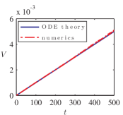
Figure 2: Acceleration of the droplet due to the inhomogeneous magnetic field $h_{0}=0.5-10^{-4}x$ with $\omega(0)=0.1$ and $\left|\mathbf{V}(0)\right|=0$. The exact solution to eq. (32) (solid) compares favorably to direct numerical simulations of the PDE (dashed).

We now demonstrate that the explicit equation (32) agrees with the previous result in Hoefer et al. (2012) obtained by perturbing conservation laws and integrating the equations numerically. Previously, the nontrivial dynamical equation was $\frac{d\mathcal{P}}{dt}=-\mathcal{N}\nabla h_{0}$. We can transform this equation into eq. (32) by using the explicit formulae (18), (16) for $\mathcal{N}$ and $\mathcal{P}$. Since $\frac{d\omega}{dT}=0$ and $\mathcal{N}$ depends only on $\omega$, $\frac{d\mathcal{N}}{dT}=0$. Then

$$\frac{d\mathcal{\boldsymbol{P}}}{dT}=\frac{\mathcal{N}^{3/2}}{\sqrt{2\pi}}\frac{d\mathbf{V}}{dT}=\frac{m_{\rm eff}}{\epsilon}\frac{d^{2}\boldsymbol{\xi}}{dt^{2}}=-\frac{\mathcal{N}}{\epsilon}\nabla h_{0}.$$ (33)

This is exactly (32). The particle-like droplet with mass $m_{\rm eff}$ in eq. (22) experiences a conservative force due to the potential $\mathcal{N}h_{0}$. This interpretation is consistent with the analysis of the effective mass derived from the kinetic energy in Section 3. Furthermore, it demonstrates that a droplet in a magnetic field gradient behaves effectively like a single magnetic dipole with net dipole moment $\mathcal{N}$.

The effect of an inhomogeneous magnetic field on a massive two-dimensional droplet is markedly different from its effect on a one-dimensional droplet Kosevich et al. (1998) and a vortex Papanicolaou and Tomaras (1991). A one-dimensional droplet experiences periodic, Bloch-type oscillations for a magnetic field with constant gradient, while a magnetic vortex exhibits motion perpendicular to the field gradient direction.

5.2 Damping

In Hoefer et al. (2012), it was observed that the droplet accelerates as it collapses in the presence of damping alone. The framework presented here offers an analytical tool to understand this slightly counterintuitive result, namely that damping can cause the otherwise steady droplet to speed up. The relevant contributions to eq. 1 are

$$p_{\Theta}=-(\omega+h_{0}-\mathbf{V}\cdot\nabla\Phi)\sin(\Theta)\mbox{ and }p_{\Phi}=-\mathbf{V}\cdot\nabla\Theta$$ (34)

where the small parameter $\epsilon$ is the Landau-Lifshitz magnetic damping parameter, usually denoted $\alpha$. In many practical situations, the damping parameter is quite small.

Evaluation of equations (23)-(26) with these perturbations yields two nontrivial equations

$$\frac{d\omega}{dT} =\omega^{2}\left(\omega+h_{0}\right)$$ (35)

$$\frac{d\mathbf{V}}{dT} =\omega\mathbf{V}\left(\omega+2h_{0}\right).$$ (36)

These equations are again consistent with the numerical, perturbed conservation law approach taken in Hoefer et al. (2012) when evaluated at the approximate solution.

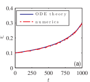
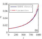
Figure 3: The evolution of droplet frequency (a) and velocity (b) due to damping for both numerical solutions of eqs. (35), (36) (solid) and direct numerical simulations of eq. (1) (dashed) when $\epsilon=\alpha=0.01$, $h_{0}=0.5$, $\omega(0)=0.1$ and $\left|\mathbf{V}(0)\right|=0.01$.

We observe that the right hand sides of the modulation equations are both positive for $h_{0}>-\omega/2$. Hence, the frequency and velocity increase. Equation (35) can be interpreted as a dynamical equation for the droplet’s mass $m_{\rm eff}$ (eq. (22)). The mass is decreasing at a faster rate than the velocity. In light of the interpretation given in Section 55.1, even though the droplet is losing energy, it sheds mass fast enough that its acceleration is not a contradiction. In Fig. 3 we see good agreement between the modulation theory and full micromagnetic simulations.

Since Eq. (35) decouples in this system, an analytical solution can be found. Elementary application of partial fractions yields an explicit solution in terms of the Lambert W-function; however, the analysis is significantly simplified when $h_{0}=0$. In this case, the analytical solution to Eqs. (35)-(36) is

$$\omega(t) =\frac{\omega_{0}}{\sqrt{1-2\alpha\omega_{0}^{2}t}},$$ (37)

$$\mathbf{V}(t) =\frac{\mathbf{V}_{0}}{\sqrt{1-2\alpha\omega_{0}^{2}t}},$$ (38)

where $\omega_{0}$ is the initial precession frequency and $\mathbf{V}_{0}$ the initial velocity. These expressions reveal two facts: a clear time of breakdown for modulation theory and the existence of an adiabatic invariant. Dividing Eq. (37) by the components of Eq. (38) demonstrates that the quantities $\omega/V_{x}$ and $\omega/V_{y}$ are constant in time.

5.3 NC-STO and Spatially Inhomogeneous Applied Field

So far, the examples we have chosen to focus on have not included higher order contributions via the phase $\Phi_{0}$ and the second term of the equation for the droplet center $\boldsymbol{\xi}$. But many perturbations and physical behaviors cannot be investigated without these higher order terms. Consider the more complex system of a nanocontact spin-torque oscillator (NC-STO), in which a polarized spin current exerts a torque on the magnetization, the spin transfer torque Berger (1996); Slonczewski (1996). This forcing can be confined to a localized region via a nanocontact Tsoi et al. (1998); Slonczewski (1999); Rippard et al. (2004). Perturbations of this sort lead to dynamics within all the parameters of the droplet. In addition to spin torque, a droplet in a NC-STO also experiences damping and it is precisely the balance between the two that leads to the stable droplet observed in experiments. Here, we consider the addition of weak spatial inhomogeneity of the applied magnetic field. For simplicity we restrict our consideration to a constant magnetic field gradient.

This investigation has broader implications for the practical use and understanding of droplets in real devices. We show in this section that these three physical effects influence the system in competing ways, which can balance, allowing for the existence of stable droplets. Alternatively, a strong enough field gradient can push the droplet out of the NC-STO, giving rise to a previously unexplained drift instability Hoefer et al. (2010). As seen in Sec. 55.2, damping decreases the effective mass of the droplet. In Sec. 55.1, it was shown that a field inhomogeneity accelerates the droplet while leaving the mass of the droplet unaffected. The inclusion of forcing due to spin transfer torque in a nanocontact opposes both of these effects. The spin torque increases the droplet mass and generates an effective restoring force that centers the droplet in the nanocontact region Bookman and Hoefer (2013). Hence, there can exist a delicate balance between all of these effects: the NC-STO restoring force balancing the potential force due to the field gradient and the mass loss due to damping balancing the mass gain due to spin-torque. Previous studies have been unable to identify when such a balance occurs and when it fails. Here, we analytically demonstrate stable droplets as fixed points of the modulation equations with all of these perturbations.

Because the perturbation components $p_{\Theta}$ and $p_{\Phi}$ appear linearly in the modulation equations (23)-(26), we can simply add the field inhomogeneity eq. (31) and damping eq. (34) perturbations to those due to spin torque Stiles and Miltat (2006). Due to the presence of three different perturbations, we no longer scale the perturbation $\mathbf{p}$ in eq. (1) by the single parameter $\epsilon$. Rather, we set $\epsilon=1$ and introduce the small parameters in $p_{\Theta}$ and $p_{\Phi}$ directly. The perturbation components are

$$p_{\Theta} =-\alpha\left(\omega+h_{0}-\mathbf{V}\cdot\nabla\Phi\right)\sin\Theta+\sigma\mathscr{H}(\rho_{*}-r)\sin\Theta,$$ (39)

$$p_{\Phi} =\left(\nabla h_{0}\cdot\hat{\boldsymbol{\rho}}\right)\rho-\alpha\mathbf{V}\cdot\nabla\Theta.$$ (40)

The nanocontact where spin torque is active is assumed to be a circle with radius $\rho_{*}$. The coordinate $r$ in the argument of the Heaviside function $\mathscr{H}$ is measured from the center of the nanocontact, which differs from the coordinates $\rho$ and $\varphi$ which are measured from the center of the droplet. For simplicity, we have neglected the spin torque asymmetry that introduces another parameter into the analysis but does not appear to have a significant effect on the dynamics Hoefer et al. (2010). Experiments Mohseni et al. (2013); Macià et al. (2014) and analysis Hoefer et al. (2010); Bookman and Hoefer (2013) have shown that the ratio of damping, $\alpha$, to forcing strength, $\sigma$ (proportional to current), is roughly order 1 for the existence of droplets to be satisfied. Thus $0<\sigma\sim\alpha\ll 1$. The magnetic field is assumed to be linear

$$h_{0}=a+bx,\quad|b|\ll\omega.$$ (41)

We can restrict to droplet motion in the $\hat{\mathbf{x}}$ direction only. Insertion of the perturbations in Eqs. (39), (40) into the modulation equations (23)- (26) results in the following system

$$\displaystyle\dot{\Phi}_{0} =\displaystyle\frac{\alpha bV}{2\omega^{2}}-\frac{\sigma V}{4\pi}\int_{|\mathbf{x}|<\rho_{*}}\cos(\varphi)\text{sech}^{2}\left(\rho-\frac{1}{\omega}\right)d\mathbf{x}$$ (42)

$$\displaystyle\dot{\xi} \displaystyle=V-\frac{\alpha b}{\omega}+\frac{\sigma\omega}{2\pi}\int_{|\mathbf{x}|<\rho_{*}}\cos(\varphi)\text{sech}^{2}\left(\rho-\frac{1}{\omega}\right)d\mathbf{x}$$ (43)

$$\displaystyle\dot{\omega} \displaystyle=\alpha\omega^{2}\left(\omega+a\right)-\frac{\sigma\omega^{3}}{4\pi}\int_{|\mathbf{x}|<\rho_{*}}\text{sech}^{2}\left(\rho-\frac{1}{\omega}\right)d\mathbf{x}$$ (44)

$$\displaystyle\dot{V} \displaystyle=-b\omega+\alpha V\omega\left(\omega+2a\right)\displaystyle-\frac{\sigma V\omega}{4\pi}\int_{|\mathbf{x}|<\rho_{*}}\frac{(3\rho\omega+\cos(2\varphi)-1)}{\rho}\text{sech}^{2}\left(\rho-\frac{1}{\omega}\right)d\mathbf{x}$$ (45)

where we set $\xi=\xi_{x}$, $V=V_{x}$, and the over dot denotes differentiation with respect to $t$. None of the right hand sides in the equations above depend explicitly on the parameter $\Phi_{0}$ so that the dynamics of the remaining parameters can be considered separately. We ignore the evolution of $\dot{\Phi}_{0}$ for the remainder of the analysis noting that $\dot{\Phi}_{0}$ corresponds to a small frequency shift as in Eq. (29) that can be obtained from the evolution of the other parameters by insertion into Eq. (42).

There is a complex interplay between the many small parameters in this problem. Since we do not have access to an exact analytical solution, it is necessary that these perturbations dominate over the error terms in our approximate solution, while still remaining small. Since we have $|V|\lesssim\omega^{2}$ to keep an overall consistent error estimate for the approximate droplet, we require that $\alpha,\sigma\ll\omega$. The variation in the applied field, $b$, is a more subtle and the appropriate scaling will be determined by directly computing fixed points.

The stationary droplet without a field gradient is stable when centered on the nanocontact Hoefer et al. (2010); Bookman and Hoefer (2013). This results from an analysis of the stationary modulation equations which exhibit an attractive, stable fixed point. Taking $\frac{dh_{0}}{dx}=b=0$, the modulation equations (43)-(45) for propagating droplets exhibit the same fixed point $(\xi,\omega,V)=(0,\omega_{*},0)$ when damping balances forcing corresponding to the current

$$\frac{\sigma}{\alpha}=\frac{2\left(a+\omega_{*}\right)}{1+\omega_{*}\left(\log\left(\frac{1}{2}\text{sech}\left(\rho_{*}-\frac{1}{\omega_{*}}\right)\right)+\rho_{*}\tanh\left(\rho_{*}-\frac{1}{\omega_{*}}\right)\right)}.$$ (46)

There is a saddle node bifurcation as $\sigma$ is increased, with $\omega_{*}=\omega_{*}(\sigma)$ corresponding to the stable branch. For $\sigma$ sufficiently large, the stable branch quickly approaches

$$\omega_{*}=\rho_{*}^{-1}+\mathrm{arctanh}\left(\frac{2a\alpha}{\sigma}-1\right)\rho_{*}^{-2}+\mathcal{O}\left(\rho_{*}^{-3}\right),\quad\rho_{*}\gg 1,\quad 0<\omega_{*}-\rho_{*}^{-1}\ll 1.$$ (47)

Near the critical value $\sigma=2a\alpha$, where the second term is small, the asymptotic form is

$$\omega_{*}=\rho_{*}^{-1}+\left(\frac{2a\alpha}{\sigma}-1\right)\rho_{*}^{-2}+\left(\frac{2\alpha}{\sigma}+\ln 2\right)\rho_{*}^{-3}+\mathcal{O}\left(\rho_{*}^{-4}\right),\quad\left|\frac{2a\alpha}{\sigma}-1\right|=\mathcal{O}\left(\rho_{*}^{-1}\right).$$ (48)

Linearizing equations (43)- (45) about this fixed point, the Jacobian matrix is given by

$$J(0,\omega_{*},0) =\left(\begin{array}[]{ccc}\lambda_{1}&0&1\\ 0&\lambda_{2}&0\\ 0&0&\lambda_{3}\\ \end{array}\right),$$ (52)

$$\lambda_{1} =-\frac{1}{2}\sigma\rho_{*}\omega_{*}\text{sech}^{2}\left(\rho_{*}-\frac{1}{\omega_{*}}\right),$$ (53)

$$\lambda_{2} =-\alpha a\omega_{*}+\lambda_{1}+\frac{1}{2}\sigma\omega_{*}\left(\tanh\left(\rho_{*}-\frac{1}{\omega_{*}}\right)+1\right),$$ (54)

$$\lambda_{3} =-2\alpha\omega_{*}^{2}+\lambda_{2}-\lambda_{1}.$$ (55)

This linearization represents a generalization of that considered in Bookman and Hoefer (2013) where the motion was restricted to $V=0$. Since $\rho_{*}>\omega_{*}^{-1}$, we observe that all eigenvalues are negative when $\sigma>a\alpha$, so the fixed point is stable. The critical forcing value $\sigma=a\alpha$, below which the droplet may be unstable could be considered as an estimate for the minimum sustaining current of a droplet Hoefer et al. (2010). Note, however, that this is a dubious estimate due to $\omega_{*}-\rho_{*}^{-1}$ not being a small quantity. Utilizing the approximation from Eq. (48), we find

$$\begin{split}\lambda_{1}&=-\frac{\sigma}{2}+\mathcal{O}\left(\rho_{*}^{-2}\right),\quad\lambda_{2}\sim\lambda_{1},\quad\lambda_{3}=\left(-\alpha+\frac{\ln 2}{2}\sigma\right)\rho_{*}^{-2}+\mathcal{O}\left(\rho_{*}^{-4}\right),\quad\left|\frac{2a\alpha}{\sigma}-1\right|=\mathcal{O}\left(\rho_{*}^{-1}\right).\end{split}$$ (56)

We now turn our attention to the case of a small field gradient $0<\left|b\right|\ll 1$, where we observe the persistence of the droplet fixed point for very small $\left|b\right|$. These fixed points exist as a balance between the expulsive force provided by the field gradient and the attractive force provided by the nanocontact. This attraction manifests in the evolution of $\xi$ and so this balance can also be viewed as a balance between leading order effects (in $V$) and higher order effects (in $\xi$). Unlike the stationary fixed point, exact analytical expressions for the fixed point cannot be found since the droplet is no longer centered on the nanocontact ($\xi\not=0$). Nevertheless, we can obtain the approximate form for these fixed points as follows. The structure of $J$ in Eq. (52) yields very simple predictions in the regime of small field gradient. The key observation here is that the system of Eqs. (43)-(45) can be written as

$$\begin{pmatrix}\dot{\xi}\\ \dot{\omega}\\ \dot{V}\end{pmatrix}=F(\xi,\omega,V)-b\begin{pmatrix}\frac{\alpha}{\omega}\\ 0\\ \omega\end{pmatrix}.$$ (57)

By virtue of the stationary fixed point, $F$ satisfies $F(0,\omega_{*},0)=0$. We now seek a fixed point that slightly deviates from the stationary one according to $\xi=b\xi_{1}+\cdots$, $\omega=\omega_{*}+b\omega_{1}+\cdots$ and $V=bV_{1}+\cdots$.

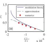
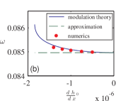
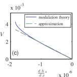
Figure 4: Fixed points from modulation theory, exact (solid) and approximate Eq. (58) (dashed), and direct numerical simulation of Eq. (1) (circles) when $\alpha=\sigma=0.01$, $a=0.5$, $\rho_{*}=12$. In this case, the parameter $V$ cannot be extracted from direct numerical simulations without additional assumptions (see Appendix A). Accordingly, this data is not presented in (c).

Expanding and equating the right hand side of Eq. (57) to zero gives the correction

$$\begin{pmatrix}\displaystyle\xi_{1}\\ \displaystyle\omega_{1}\\ \displaystyle V_{1}\end{pmatrix}=J(0,\omega_{*},0)^{-1}\begin{pmatrix}\frac{\alpha}{\omega_{*}}\\ 0\\ w_{*}\end{pmatrix}=\begin{pmatrix}\frac{\alpha}{\lambda_{1}\omega_{*}}-\frac{\omega_{*}}{\lambda_{1}\lambda_{3}}\\ 0\\ \frac{\omega_{*}}{\lambda_{3}}\end{pmatrix}\sim\begin{pmatrix}\frac{4\rho_{*}}{-2\alpha\sigma+\sigma^{2}\ln 2}\\ 0\\ \frac{2\rho_{*}}{-2\alpha+\sigma\ln 2}\end{pmatrix},$$ (58)

where the approximations (48) and (56) were used to obtain the large $\rho_{*}$ estimate. These approximations are valid so long as $\sigma$ is more than $\rho_{*}^{-2}$ away from the critical value $2\alpha/\ln 2\approx 2.9\alpha$. Otherwise, higher order terms in Eq. (56) would need to be considered.

As summarized in Fig. 4, these simple expressions make predictions in good agreement with the fixed points found by numerical continuation in $b$ and those observed in long time micromagnetic simulations of Eq. (1) with perturbations (39) and (40). The Jacobian matrix of Eqs. (43)-(45) can also be numerically evaluated, showing that all eigenvalues are negative, until continuation breaks down when one eigenvalue reaches zero. After this bifurcation, we do not find any fixed points. The condition of this eigenvalue reaching zero then corresponds exactly to the crossover where the attractive nanocontact is no longer strong enough to balance the expulsive force supplied by the field gradient. If we assume that a field gradient is strong enough to move the droplet an order one distance, still small relative to the droplet radius $\omega_{*}^{-1}$, then we obtain a typical field gradient scaling $b\approx\alpha\sigma/2\rho_{*}$. This field gradient is very small. For the example studied here, $b\approx 10^{-6}$ compared to the NC-STO forcing magnitude $\sigma=10^{-2}$. This demonstrates that droplet attraction due to spin torque is weak relative to droplet acceleration due to field inhomogeneity. A strong enough field gradient, on the scale of $\alpha\sigma/2\rho_{*}$, can eject the droplet from the nanocontact, causing a drift instability previously observed in numerical simulations Hoefer et al. (2010). Additionally, the associated velocity scale from Eq. (58) is $V=bV_{1}\sim\sigma/2$ which is much smaller than $\omega$ as required for this order of accuracy of the approximate droplet.

6 Interacting Droplets

An intriguing, indeed defining, aspect of solitary wave dynamics is their interaction behavior. Reference Maiden et al. (2014) undertook a numerical investigation of two interacting droplets by varying droplet parameters and quantifying the properties of the solution post-interaction. It was found that the relative phase difference between the two droplets plays a fundamental role, controlling whether the interaction is attractive or repulsive. The attractive interactions studied were strongly nonlinear, hence a perturbation theory would be insufficient to study the full complement of observed phenomena. Nevertheless, we can gain insight into the nature of the interaction (attractive/repulsive) by studying two well-separated droplets perturbatively, with the small parameter being the inverse of the droplet separation. This approach is well-known and has been applied successfully to, for example, NLS-type models Zhu and Yang (2007); Ablowitz et al. (2009).

In full generality, the perturbations arising from this analysis are complex. However, since the validity of these equations is strongly dependent on the separation of the two droplets, we only expect these equations to be valid over short time scales. Hence, we only seek to describe the initial behavior of two stationary, weakly overlapping droplets. As the interaction immediately excites propagation of the two droplets, this will not model the behavior for $t>0$. Nevertheless, these assumptions make it possible to describe much of the behavior observed in full numerical simulations Maiden et al. (2014). The initial configuration places one droplet on the left (subscripted $1$) and another droplet (subscripted $2$) a distance $d$ away along the $x-$axis. We define the relative phase difference $\Delta\Phi=\Phi_{2}-\Phi_{1}$, which will emerge as an important quantity in the modulation equations. Considering the modulation equations for two weakly interacting droplets with motion in the $\hat{\mathbf{x}}$ direction at the initial time only yields

$$\displaystyle\dot{\Phi}_{0,k} \displaystyle=-\frac{\omega}{2\pi}\cos(\Delta\Phi)\int_{\mathbb{R}^{2}}\mathcal{K}_{k}(\mathbf{x})d\mathbf{x},$$ (59)

$$\displaystyle\dot{\xi}_{k} \displaystyle=\frac{\omega}{2\pi}(-1)^{k+1}\sin(\Delta\Phi)\int_{\mathbb{R}^{2}}\mathcal{K}_{k}(\mathbf{x})\text{sech}\left(\rho-\frac{1}{\omega}\right)\cos\varphi d\mathbf{x},$$ (60)

$$\displaystyle\dot{\omega}_{k} \displaystyle=-\frac{\omega^{3}}{4\pi}(-1)^{k+1}\sin(\Delta\Phi)\int_{\mathbb{R}^{2}}\mathcal{K}_{k}(\mathbf{x})\text{sech}\left(\rho-\frac{1}{\omega}\right)d\mathbf{x},$$ (61)

$$\displaystyle\dot{V}_{k} \displaystyle=\frac{\omega^{3}}{\pi}\cos(\Delta\Phi)\int_{\mathbb{R}^{2}}\mathcal{K}_{k}(\mathbf{x})\cos\varphi d\mathbf{x},$$ (62)

where

$$\mathcal{K}_{k}(\mathbf{x}) =\text{sech}\left(\tilde{\rho}_{k}-\frac{1}{\omega}\right)\text{sech}\left(\rho-\frac{1}{\omega}\right)\times\left[2\text{sech}^{2}\left(\rho-\frac{1}{\omega}\right)-\omega\left(1-\tanh\left(\rho-\frac{1}{\omega}\right)\right)\right].$$ (63)

The integration kernel $\mathcal{K}_{k}$ depends on the separation between the two droplets through $\tilde{\rho}_{k}=\sqrt{(x+(-1)^{k}d)^{2}+y^{2}}$. Utilizing this framework, we can now offer some insight into the nature of two interacting droplets.

6.1 Attraction and Repulsion

The attractive or repulsive nature of two droplets can be understood by considering Eq. 62. As $\Delta\Phi$ varies, the sign of $\cos(\Delta\Phi)$ is clear. Determining the initial direction of motion, right or left, of the droplet comes down to determining the sign of the integral term in (62).

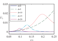
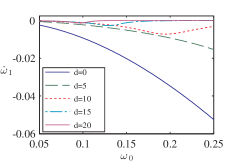
Figure 5: Left: Initial acceleration for varied initial $\omega$ and several values of separation. Right: Plot of $\dot{\omega}_{1}$ as a function of initial $\omega_{0}$ for several values of separation. In both, the initial relative phase was $\Delta\Phi=1$.

Figure 5, left shows the numerical evaluation of the right hand side of $\dot{V}_{1}$ (droplet on left) when $\Delta\Phi=1<\pi/2$, leading to positive values only. Thus, the left droplet experiences a positive acceleration to the right, towards the other droplet when $|\Delta\Phi|<\pi/2$. Since the kernel exhibits the symmetry with respect to droplet choice $\mathcal{K}_{1}(x,y)=\mathcal{K}_{2}(-x,y)$, the integral in (62) for the right droplet, $k=2$, has the opposite sign. The right droplet experiences a negative acceleration to the left when $|\Delta\Phi|<\pi/2$. Therefore, two droplets are attractive when $|\Delta\Phi|<\pi/2$, i.e., when they are sufficiently in phase. Similarly, when $\pi/2<|\Delta\Phi|<\pi$, the signs of $\dot{V}_{k}$ are reversed and the droplets move away from each other. Thus, two droplets are repulsive when they are sufficiently out of phase.

As was noted in Maiden et al. (2014) by a nonlinear method of images, the attractive or repulsive nature of two droplets with the special initial values $\Delta\Phi=0$ or $\Delta\Phi=\pi$ describes the behavior of a single droplet near a magnetic boundary with either a free spin (Neumann type) boundary condition or a fixed spin (Dirichlet type) boundary condition, respectively. The analysis presented here confirms this fact for any droplet that weakly interacts with a magnetic boundary. Such behavior was observed in micromagnetic simulations of a droplet in a NC-STO, nanowire geometry Iacocca et al. (2014).

6.2 Asymmetry

Despite a highly symmetric initial condition, an asymmetry was observed in so-called “head-on collisions" of two droplets in Maiden et al. (2014). The frequency equation (61) provides an explanation of this in the limit of very small velocities. Figure 5, right contains the relevant information. Since $\dot{w}_{1}$ appears to be negative always when $\sin(\Delta\Phi)>0$. In the numerical experiments in Maiden et al. (2014) were done over the range $\Delta\Phi=0$ to $\Delta\Phi=\pi$, this was always the case. Again using that $\mathcal{K}_{1}(x,y)=\mathcal{K}_{2}(-x,y)$, it can be seen that the integrals involved in computing $\dot{\omega}_{1}$ and $\dot{\omega}_{2}$ are equal. Hence the sign of $\dot{\omega}_{k}$ is determined by $(-1)^{k+1}$, and the signs of $\dot{\omega}_{1}$ and $\dot{\omega}_{2}$ will always be opposite. For the parameters discussed here, this means that the frequency decreases for the droplet on the left and increases on the right. This change in droplet structure is asymmetric because a reduced (increased) frequency implies larger (smaller) droplet mass and corresponds precisely with the observations of Maiden et al. (2014).

6.3 Acceleration

The discussion of attraction and repulsion in Section 66.1 suggests that the boundary between the two behaviors is $\Delta\Phi=\pi/2$. But this does not agree with numerical experiments where the crossover $\Delta\Phi$ was found to vary with the initial droplet parameters Maiden et al. (2014). To offer an explanation for this, we consider the total acceleration of the initial droplets, i.e., $\ddot{\xi}_{k}$. This incorporates higher order information not included in $\dot{V}_{k}$. Since the full modulation equations for interacting droplets when $V\neq 0$ are complex, we do not examine $\ddot{\xi}_{k}$ for all values of $\Delta\Phi$. However, at $\Delta\Phi=\frac{\pi}{2}$, we know $\dot{V}_{k}=\dot{\Phi}_{0}=0$, (since $\cos(\Delta\Phi)=0$) and those terms will not contribute, which simplifies the calculation. Figure 6 shows the initial, total droplet acceleration $\ddot{\xi}_{1}$, evaluated numerically, as the initial frequency and separation are varied.

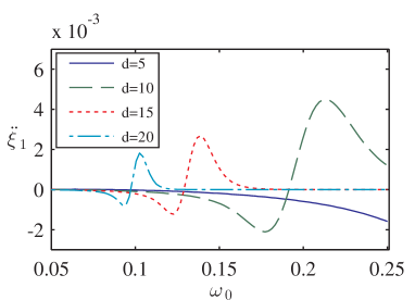
Figure 6: Numerical evaluation of $\ddot{\xi}_{1}$ initially for $\Delta\Phi=\pi/2$, variable droplet separation $d$ and frequency $\omega_{0}$. There is not one sign of acceleration, i.e., the left droplet can be repelled or attracted to the right droplet depending on the choice of parameters.

The variable sign of this quantity as parameters change demonstrates that subtle, higher order effects causes the crossover value of $\Delta\Phi$ to deviate from its nominal value $\pi/2$.

7 Conclusion

The primary contribution of this work is a general framework for investigating perturbations of droplet solitons. Actual physical devices used to create and manipulate droplets are quite complex, incorporating a number of physical effects. Therefore, having a tractable, analytical theory to describe both the motion and precession of droplets due to physical perturbations is quite valuable. The examples presented here are meant to demonstrate the versatility and power of this tool. Additionally, the application of this theory to the NC-STO provides several insights into the behavior of experimentally observed dissipative droplets. In particular, the dissipative droplet is shown to be robust in the presence of weak field gradients, but can be ejected from the nanocontact if the field gradient is too large, providing an explanation for a previously observed drift instability. These observations open possible mechanisms for generating a current of solitons which could serve as a mechanism for information transfer.

As demonstrated by examples in the preceding sections, many perturbations excite evolution of higher order parameters (overall phase and position). This subtle information proves to be of fundamental importance for several perturbations considered. As shown by our derivation of the modulation equations for a general class of Hamiltonian systems, the higher order parameter dynamics emerge when the generalized nullspace of the linearized evolution operator is incorporated. Due to the existence of an approximate analytical form for the propagating droplet, we are able to completely characterize this nullspace and hence recover the droplet modulation equations in a convenient form.

A number of physical perturbations can now be investigated within this framework. Future developments of the modulation theory itself could be performed in the context of a different family of magnetic droplet solutions. One example is the weakly nonlinear droplet Ivanov et al. (2001). Recent micromagnetic simulations have found rotating and precessing localized waves in NC-STOs with non-trivial magnetostatic contributions Finocchio et al. (2013). The invariance of equation (1) when $\epsilon=0$ with respect to rotation of the domain and an analysis of conserved quantities Papanicolaou and Tomaras (1991), suggests that there may be rotating and precessing solitary wave solutions. The modulation theory developed in this work could be extended to such solitary wave solutions.

Appendix A Numerical Method

The numerical simulations (micromagnetics) we conducted incorporated a periodic Fourier psuedospectral spatial discretization. Unless otherwise stated, the spatial domain was $[-50,50]\times[-50,50]$, sufficiently large so that the perturbed solitary waves were well-localized within it. In each spatial dimension, $2^{9}$ grid points were used. The time-stepping was done using a version of the Runge-Kutta-Fehlberg algorithm, modified so that the magnetization maintained unit length at every grid point and each time step.

The velocity, $\mathbf{V}$, was extracted from numerical data by computing the center of mass, $\boldsymbol{\xi}(t)=\int_{\mathbb{R}^{2}}\mathbf{x}(1-m_{3}(\mathbf{x},t))d\mathbf{x}/\mathcal{N}$. We then estimated $\mathbf{V}=\dot{\boldsymbol{\xi}}$, approximated using a forward difference of $\boldsymbol{\xi}(t)$. This method does not work for perturbations which excite higher order changes in $\dot{\boldsymbol{\xi}}$ and we do not estimate $\mathbf{V}$ in such cases.

For the precessional frequency $\omega$, the phase of the in-plane magnetization $(m_{x},m_{y})$ was extracted at a point a fixed distance from the center of mass $\boldsymbol{\xi}$. Differentiating this phase with respect to time yields $\Omega(t)$ as in Eq. (29). The precessional frequency, $\omega$, was obtained by subtracting $h_{0}$ and $\dot{\Phi}_{0}$. The contribution from $\dot{\Phi}_{0}$ was estimated via the modulation equation (23). An alternative method based on computing the conserved quantities in Eqs. (15)-(16) was used for comparison. The relations for total spin and momentum of the approximate droplet Eqs. (18)-(19) were inverted to obtain $\omega$ and $\mathbf{V}$. The two methods were in good agreement.

Appendix B Approximate Droplet

As noted in the main body of the manuscript, the derivation of the approximate droplet is significantly simplified by exploiting the invariance of Eq. (11) under rotation of the domain and working in the frame where $V_{y}=0$ and $\mathbf{V}=V_{x}\hat{\mathbf{x}}\equiv V\hat{\mathbf{x}}$. The derivation proceeds by substituting the ansatz

$$\Theta=\Theta_{0}(\rho)+V\Theta_{1}(\rho,\varphi)+\mathcal{O}\left(V^{2}\right)\mbox{ and }\Phi=\Phi_{0}+V\Phi_{1}(\rho,\varphi)+\mathcal{O}\left(V^{2}\right)$$ (64)

into Eq. (11). At order $\mathcal{O}\left(1\right)$, this yields one nontrivial equation,

$$\frac{d^{2}\Theta_{0}}{d\rho^{2}}+\frac{1}{\rho}\frac{d\Theta_{0}}{d\rho}+\left(\omega-\cos\right)\sin(\Theta_{0})=0.$$ (65)

This equation has been extensively studied and is known to admit an approximate solution in the limit of $0<\omega\ll 1$, $\Theta_{0}=\arccos\left(\tanh\left(\rho-\frac{1}{\omega}\right)\right)+\mathcal{O}\left(\omega^{2}\right)$ Ivanov and Stephanovich [1989], Kosevich et al. [1986], Bookman and Hoefer [2013]. From here on out, we additionally assume that $0<\omega\ll 1$. At order $\mathcal{O}\left(V\right)$, we find

$$\sin(\Theta_{0})\Delta\Phi_{1}+\left(\cos(\varphi)+2\cos(\Theta_{0})\frac{\partial\Phi_{1}}{\partial\rho}\right)\frac{d\Theta_{0}}{d\rho}=0,$$ (66)

$$\Delta\Theta_{1}+\left(\omega\cos\left(\Theta_{0}\right)-\cos\left(2\Theta_{0}\right)\right)\Theta_{1}=0.$$ (67)

Equation (67) is solved by $\Theta_{1}=0$. Substituting the approximate solution for $\Theta_{0}$ into Eq. (66)

$$\left(\Delta\Phi_{1}-\cos(\varphi)-2\tanh\left(\rho-\frac{1}{\omega}\right)\frac{\partial\Phi_{1}}{\partial\rho}\right)\text{sech}\left(\rho-\frac{1}{\omega}\right)=0$$ (68)

The residual in Eq. (68) is determined by two considerations. If $1\ll\rho-\omega^{-1}$, $\text{sech}\left(\rho-1/\omega\right)$ dominates and the residual is exponentially small. In the other case, i.e. $\rho\sim\omega^{-1}$, the residual will only be small if $\Delta\Phi_{1}-\cos(\varphi)-2\tanh\left(\rho-1/\omega\right)\frac{\partial\Phi_{1}}{\partial\rho}$ is small since $\text{sech}\left(\rho-1/\omega\right)$ is $\mathcal{O}\left(1\right)$. This suggests that the boundary condition, $\lim_{\rho}\nabla\Phi_{1}=\frac{1}{2}\hat{\mathbf{x}}$, may be neglected. Assuming $\Phi_{1}$ is separable of the form $\Phi_{1}(\rho,\varphi)=f(\rho)\cos(\varphi)$, Eq. (68) simplifies to the ordinary differential equation

$$\frac{d^{2}f}{d\rho^{2}}+\left(\frac{1}{\rho}-2\tanh\left(\rho-\frac{1}{\omega}\right)\right)\frac{df}{d\rho}-\frac{1}{\rho^{2}}f=1.$$ (69)

Numerical solutions of Eq. (69) demonstrate that $f$ becomes quite large, approximately $\mathcal{O}\left(\frac{1}{\omega^{2}}\right)$ near $\rho=\frac{1}{\omega}$. Factoring this into the analysis, we change to the coordinate system $R=\rho-\frac{1}{\omega}$ and expand $f$ in the series

$$f(\rho)=\frac{f_{0}(\rho)}{\omega^{2}}+\frac{f_{1}(\rho)}{\omega}+f_{2}(\rho)+\cdots.$$ (70)

Let $L\equiv\frac{d^{2}}{dR^{2}}-2\tanh(R)\frac{d}{dR}$. Substituting the ansatz in Eq. (70) into Eq. (69) yields,

$$\mathcal{O}\left(\frac{1}{\omega^{2}}\right): Lf_{0} =0$$ (71)

$$\mathcal{O}\left(\frac{1}{\omega}\right): Lf_{1} =-\frac{df_{0}}{dR}$$ (72)

$$\mathcal{O}\left(1\right): Lf_{2} =-\frac{df_{1}}{dR}+1+f_{0}+R\frac{df_{0}}{dR}$$ (73)

Eq. (71) admits any constant solution. Take $f_{0}=A$. Substituting this expression for $f_{0}$ into Eq. (72), yields $Lf_{1}=0$. Thus, any constant solution is admissible for $f_{1}$ as well. Take $f_{1}=B$. Substituting these expressions for $f_{0}$ and $f_{1}$ into Eq. (73), yields $Lf_{2}=1+A$. However, constant solutions are in the kernel of $L$, so solvability of this equation requires $A=-1$. Similarly, solvability at $\mathcal{O}\left(\omega\right)$ requires $B=0$. Hence, we take $f(\rho)=-\frac{1}{\omega^{2}}$, which gives rise to the form of the approximate droplet in Eq. (13).

Since $\Phi$ enters into Eq. 11 only in the form of $\nabla\Phi$, the asymptotic approximations here are valid provided that $\nabla{\Phi}$ remains small. This condition is not equivalent $V\Phi_{1}\ll\Phi_{0}$. Given the form of the approximation for $f$, the small gradient condition requires that $\left|\nabla\Phi\right|=\left|\frac{V}{\omega^{2}}\frac{\sin\varphi}{\rho}\right|\ll 1$. Since the approximation is localized at $\rho\sim\omega^{-1}$, we require $V\ll\omega$.

References

- Ablowitz and Segur [1981] M. J. Ablowitz and H. Segur. Solitons and the inverse scattering transform, volume 4. SIAM, 1981.
- Ablowitz et al. [2009] M. J. Ablowitz, T. P. Horikis, S. D. Nixon, and Y. Zhu. Asymptotic analysis of pulse dynamics in mode-locked lasers. Stud. Appl. Math., 122(4):411–425, 2009.
- Ablowitz et al. [2011] M. J. Ablowitz, S. D. Nixon, T. P. Horikis, and D. J. Frantzeskakis. Perturbations of dark solitons. Proc. R. Soc. A-Math. Phys., 467(2133):2597 –2621, 2011.
- Babich and Kosevich [2001] I. M. Babich and A. M. Kosevich. Relaxation of bloch oscillations of a magnetic soliton in a nonuniform magnetic field. Low Temp. Phys., 27:35–39, 2001.
- Berger [1996] L. Berger. Emission of spin waves by a magnetic multilayer traversed by a current. Phys. Rev. B, 54(13):9353, 1996.
- Bookman and Hoefer [2013] L. D. Bookman and M. A. Hoefer. Analytical theory of modulated magnetic solitons. Phys. Rev. B, 88(18):184401, 2013.
- Chung et al. [2014] S. Chung, S. M. Mohseni, S. R. Sani, E. Iacocca, R. K. Dumas, T. N. Anh Nguyen, Ye Pogoryelov, P. K. Muduli, A. Eklund, M. Hoefer, and J. Åkerman. Spin transfer torque generated magnetic droplet solitons (invited). J. Appl. Phys., 115:172612, 2014.
- Fert et al. [2013] A. Fert, V. Cros, and J. Sampaio. Skyrmions on the track. Nature nanotechnology, 8(3):152–156, 2013.
- Finocchio et al. [2013] G. Finocchio, V. Puliafito, S. Komineas, L. Torres, O. Ozatay, T. Hauet, and B. Azzerboni. Nanoscale spintronic oscillators based on the excitation of confined soliton modes. J. Appl. Phys., 114(16):163908, 2013.
- Grillakis et al. [1990] M. Grillakis, J. Shatah, and W. Strauss. Stability theory of solitary waves in the presence of symmetry, ii. J. Funct. Anal., 94(2):308–348, 1990.
- Hoefer and Sommacal [2012] M. A. Hoefer and M. Sommacal. Propagating two-dimensional magnetic droplets. Physica D, 241(9):890–901, 2012.
- Hoefer et al. [2010] M. A. Hoefer, T. J. Silva, and M. W. Keller. Theory for a dissipative droplet soliton excited by a spin torque nanocontact. Phys. Rev. B, 82(5):054432, 2010.
- Hoefer et al. [2012] M. A. Hoefer, M. Sommacal, and T. J. Silva. Propagation and control of nanoscale magnetic-droplet solitons. Phys. Rev. B, 85(21):214433, 2012.
- Iacocca et al. [2014] E. Iacocca, R. K. Dumas, L. Bookman, M. Mohseni, S. Chung, M. A. Hoefer, and J. Åkerman. Confined dissipative droplet solitons in spin-valve nanowires with perpendicular magnetic anisotropy. Phys. Rev. Lett., 112(4):047201, 2014.
- Ivanov and Stephanovich [1989] B. A. Ivanov and V. A. Stephanovich. Two-dimensional soliton dynamics in ferromagnets. Phys. Lett. A, 141(1):89–94, 1989.
- Ivanov et al. [2001] B. A. Ivanov, C. E. Zaspel, and I. A. Yastremsky. Small-amplitude mobile solitons in the two-dimensional ferromagnet. Phys. Rev. B, 63(13):134413, 2001.
- Keener and McLaughlin [1977] J. P. Keener and D. W. McLaughlin. Solitons under perturbations. Phys. Rev. A, 16:777, 1977.
- Kevrekidis et al. [2008] P. G. Kevrekidis, D. J. Frantzeskakis, and R. Carretero-González. Emergent nonlinear phenomena in Bose-Einstein condensates : theory and experiment. Springer, 2008.
- Kivshar and Malomed [1989] Y. S. Kivshar and B. A. Malomed. Dynamics of solitons in nearly integrable systems. Rev. Mod. Phys., 61(4):763, 1989.
- Kosevich et al. [1986] A. M. Kosevich, B. A. Ivanov, and A. S. Kovalev. Sov. Sci. Rev., Sect. A, Phys. Rev., 6:171, 1986.
- Kosevich et al. [1990] A. M. Kosevich, B. A. Ivanov, and A. S. Kovalev. Magnetic solitons. Physics Reports, 194(3):117–238, 1990.
- Kosevich et al. [1998] A. M. Kosevich, V. V. Gann, A. I. Zhukov, and V. P. Voronov. Magnetic soliton motion in a nonuniform magnetic field. J. Exp. Theor. Phys., 87:401–407, 1998.
- Macià et al. [2014] F. Macià, D. Backes, and A. D. Kent. Stable magnetic droplet solitons in spin-transfer nanocontacts. Nat. Nanotechnol., 9(12):992–996, 2014.
- Maiden et al. [2014] M. D. Maiden, L. D. Bookman, and M. A. Hoefer. Attraction, merger, reflection, and annihilation in magnetic droplet soliton scattering. Phys. Rev. B, 89(18):180409, 2014.
- Mohseni et al. [2013] S. M. Mohseni, S. R. Sani, J. Persson, T. N. Anh Nguyen, S. Chung, Y. Pogoryelov, P. K. Muduli, E. Iacocca, A. Eklund, R. K. Dumas, S. Bonetti, Deac A., M. A. Hoefer, and J. Åkerman. Spin torque–generated magnetic droplet solitons. Science, 339(6125):1295–1298, 2013.
- Mohseni et al. [2014] S. M. Mohseni, S. R. Sani, R. K. Dumas, J. Persson, T. N. Anh Nguyen, S. Chung, Ye. Pogoryelov, P. K. Muduli, E. Iacocca, A. Eklund, and J. Åkerman. Magnetic droplet solitons in orthogonal nano-contact spin torque oscillators. Physica B, 435:84–87, 2014.
- Nagaosa and Tokura [2013] N. Nagaosa and Y. Tokura. Topological properties and dynamics of magnetic skyrmions. Nat. Nanotechnol., 8(12):899–911, 2013.
- Papanicolaou and Tomaras [1991] N. Papanicolaou and T. N. Tomaras. Dynamics of magnetic vortices. Nucl. Phys. B, 360(2):425–462, 1991.
- Piette and Zakrzewski [1998] B. Piette and W. J. Zakrzewski. Localized solutions in a two-dimensional landau-lifshitz model. Physica D, 119(3):314–326, 1998.
- Pulecio et al. [2014] J. F. Pulecio, P. Warnicke, S. D. Pollard, D. A. Arena, and Y. Zhu. Coherence and modality of driven interlayer-coupled magnetic vortices. Nat. Commun., 5, 2014.
- Rippard et al. [2004] W. H Rippard, M. R Pufall, S. Kaka, S. E Russek, and T. J Silva. Direct-current induced dynamics in Co90Fe10/Ni80Fe20. Phys. Rev. Lett., 92(2):027201, 2004.
- Sanchez and R. [1998] A. Sanchez and Bishop A. R. Collective coordinates and length-scale competition in spatially inhomogeneous soliton-bearing equations. SIAM Rev., 40(3):579–615, 1998.
- Slonczewski [1996] J. C. Slonczewski. Current-driven excitation of magnetic multilayers. J. Magn. Magn. Mater., 159(1):L1–L7, 1996.
- Slonczewski [1999] J. C. Slonczewski. Excitation of spin waves by an electric current. J. Magn. Magn. Mater., 195:L261–L268, 1999.
- Stiles and Miltat [2006] M. D. Stiles and J. Miltat. Spin transfer torque and dynamics. In B. Hillebrands and A. Thiaville, editors, Spin Dynamics in Confined Magnetic Structures III. Springer, Berlin, Heidelberg, 2006.
- Tsoi et al. [1998] M. Tsoi, A. G. M. Jansen, J. Bass, W.-C. Chiang, M. Seck, V. Tsoi, and P. Wyder. Excitation of a magnetic multilayer by an electric current. Phys. Rev. Lett., 80(19):4281–4284, 1998.
- Uhlíř et al. [2013] V. Uhlíř, M. Urbánek, L. Hladík, J. Spousta, M.-Y. Im, P. Fischer, N. Eibagi, J. J. Kan, E. E. Fullerton, and T. Šikola. Dynamic switching of the spin circulation in tapered magnetic nanodisks. Nat. Nanotechnol., 8(5):341–346, 2013.
- Vakhitov and Kolokolov [1973] N. G. Vakhitov and A. A. Kolokolov. Stationary solutions of the wave equation in a medium with nonlinearity saturation. Radiophys. Quantum Electron., 16(7):783–789, 1973.
- Weinstein [1985] M. I. Weinstein. Modulational stability of ground states of nonlinear schrödinger equations. SIAM J. Math. Anal., 16(3):472–491, 1985.
- Yang [2010] J. Yang. Nonlinear Waves in Integrable and Nonintegrable Systems. Society for Industrial and Applied Mathematics, 2010.
- Yu et al. [2014] X. Z. Yu, Y. Tokunaga, Y. Kaneko, W. Z. Zhang, K. Kimoto, Y. Matsui, Y. Taguchi, and Y. Tokura. Biskyrmion states and their current-driven motion in a layered manganite. Nat. Commun., 5, 2014.
- Zhu and Yang [2007] Y. Zhu and J. Yang. Universal fractal structures in the weak interaction of solitary waves in generalized nonlinear schrödinger equations. Phys. Rev. E, 75(3):036605, 2007.