Precise Radial Velocity Measurements for Kepler Giants Hosting Planetary Candidates: Kepler-91 and KOI-1894

Abstract

We present results of radial-velocity follow-up observations for the two Kepler evolved stars Kepler-91 (KOI-2133) and KOI-1894, which had been announced as candidates to host transiting giant planets, with the Subaru 8.2m telescope and the High Dispersion Spectrograph (HDS). By global modeling of the high-precision radial-velocity data taken with Subaru/HDS and photometric ones taken by Kepler mission taking account of orbital brightness modulations (ellipsoidal variations, reflected/emitted light, etc.) of the host stars, we independently confirmed that Kepler-91 hosts a transiting planet with a mass of $0.66\mbox{M${}_{\rm Jup}$}$ (Kepler-91b), and newly detected an offset of $\sim$20 m s^-1 between the radial velocities taken at $\sim 1$-yr interval, suggesting the existence of additional companion in the system. As for KOI-1894, we detected possible phased variations in the radial velocities and light curves with 2–3$\sigma$ confidence level which could be explained as a reflex motion and ellipsoidal variation of the star caused by the transiting sub-saturn-mass ($\sim 0.18\mbox{M${}_{\rm Jup}$}$) planet.

1. Introduction

Detecting planetary transits is highly valuable not only because it makes an independent confirmation of a planet from radial-velocity observations but also because the photometric transits provide unambiguous information on planet masses and radii, and thus mean density and interior structure (e.g. Winn, 2011, and references therein). Various high-precision follow-up studies for transiting planets can also uncover planetary atmospheres and the (mis-)alignment between the stellar spin and planetary orbital axes via the Rossiter-McLaughlin effect (e.g. Seager & Deming, 2010; Winn, 2011). These properties of transiting planets provide valuable hints for planet formation and evolution processes including dynamical interaction between planets.

Although transiting planets are as such important, it is difficult to detect them around evolved stars, especially giant stars, due to the large sizes of the host stars. Targets for on-going radial-velocity surveys for planets around giants have typical radii of $\sim$10 R_⊙ (e.g., da Silva et al., 2006; Takeda et al., 2008; Liu et al., 2010; Wang et al., 2011; Zielinski et al., 2012), and then the relative flux variation of such a giant host star caused by a transit of a Jupiter-sized planet is only $\sim 1\times 10^{-4}$, which is comparable to that for transit of an Earth-sized planet across a solar-type star. It is impossible to detect such a transit from ground-based photometry and thus no transiting planets had been found around giant stars. Our understanding of properties of planets around such stars are thus far behind from those around solar-like stars, although tens of planets have been found around giants by precise radial-velocity surveys (e.g. Sato et al., 2013, and references therein).

The Kepler mission was successful in detecting transiting planets with very high photometric precision ($\sim 2\times 10^{-5}$) since 2009. To date it has discovered more than 4000 transiting planet candidates from sub-Earth-size to super-Jupiter-size in $\sim$0.3–2000 d orbits (e.g. Batalha et al., 2013). Although most of them are orbiting solar-type stars, Kepler’s photometric precision is high enough to detect a Jupiter-sized planet transiting a giant star.

As expected, Kepler has identified several planet candidates around giant stars with radii larger than $5~{}R_{\odot}$ (Batalha et al., 2013). The planet candidates have radii comparable to or larger than Jupiter’s, and it is interesting that many of them have short-period orbits. Since such short-period planets have rarely been found by radial-velocity surveys around evolved stars (e.g. Johnson et al., 2007; Sato et al., 2008; Jones et al., 2014), they will provide us unique opportunities to investigate planet formation and evolution processes around such stars.

Here we report the results of radial-velocity follow-up observations using Subaru 8.2m telescope for two of the Kepler evolved stars, Kepler-91 (KOI-2133) and KOI-1894. Thanks to the high precision in their radial-velocity measurements, we independently confirmed a jovian planet (Kepler-91b, KOI-2133.01) previously reported around Kepler-91 (Lillo-Box et al., 2014a, b; Barclay et al., 2014) and newly found a hint for the existence of additional companion in the system. We also detected a possible sub-saturn-mass planet around KOI-1894 (KOI-1894.01) with 2–3$\sigma$ confidence level.

The rest of the paper is organized as follows. The adopted stellar parameters for the two stars are presented in section 2. The observations are described in section 3 and the results of global analysis for the radial velocities and light curves are presented in section 4. Section 5 is devoted to discussion and summary.

2. Targets

Kepler-91 (KIC 8219268, KOI-2133; $K_{p}$=12.495) was identified as a candidate star hosting a transiting short-period jupiter-sized planet (KOI-2133.01; $R_{p}=18.24~{}R_{\oplus}$, $P=6.2465798\pm 0.0000821$ d) by Batalha et al. (2013). After that, Lillo-Box et al. (2014a) reported the confirmation of its planetary nature based on the detailed analysis of orbital brightness modulation seen in the light curve caused by ellipsoidal variation, Doppler boosting, and reflected/emitted light from planet (e.g. Faigler & Mazeh, 2011; Mazeh et al., 2012), and then the planet was named Kepler-91b with the radius $R_{p}=1.384^{+0.011}_{-0.054}~{}\mbox{R${}_{\rm Jup}$}$ and mass $M_{p}=0.88^{+0.17}_{-0.33}~{}\mbox{M${}_{\rm Jup}$}$. Although Esteves et al. (2013) and Sliski & Kipping (2014) claimed a possible non-planertary nature for the system, Lillo-Box et al. (2014b) and Barclay et al. (2014) very recently reconfirmed the planetary nature via radial-velocity measurements with a precision of $\sim$100 m s^-1 and $\sim$20 m s^-1, respectively, and obtained the planetary mass of 1.09$\pm$0.20M_Jup and 0.73$\pm$0.13M_Jup, respectively.

The stellar parameters (effective temperature $T_{\rm eff}$, surface gravity $\log g$, mass $M_{\star}$, and radius $R_{\star}$) of Kepler-91 were reported by Batalha et al. (2013) to be $T_{\rm eff}=4712$ K, $\log g=2.85$ cgs, $M_{\star}=2.25~{}M_{\odot}$, and $R_{\star}=9.30~{}R_{\odot}$. After that, the parameters have been updated by the spectroscopic and asteroseismic analyses in Huber et al. (2013a) and Lillo-Box et al. (2014a), which are consistent with each other. Thus, we here adopted the values listed in Lillo-Box et al. (2014a): $T_{\rm eff}=4550\pm 75$ K, $\log g=2.953\pm 0.007$ cgs, $M_{\star}=1.31\pm 0.10~{}M_{\odot}$, and $R_{\star}=6.30\pm 0.16~{}R_{\odot}$.

KOI-1894 (KIC 11673802; $K_{p}$=13.427) was also reported to be a planet-host candidate having a transiting short-period jupiter-sized planet (KOI-1894.01; $R_{p}=16.29~{}R_{\oplus}$, $P=5.2880157\pm 0.0000447$ d) by Batalha et al. (2013), though radial-velocity follow-up observations for the star have not been reported yet. The stellar parameters of KOI-1894 were derived by Batalha et al. (2013) to be $T_{\rm eff}=4815$ K, $\log g=2.87$ cgs, $M_{\star}=2.02~{}M_{\odot}$, and $R_{\star}=8.62~{}R_{\odot}$, and they have been updated by the spectroscopic and asteroseismic analyses in Huber et al. (2013a) as $T_{\rm eff}=4992\pm 75$ K, $M_{\star}=1.410\pm 0.214~{}M_{\odot}$, and $R_{\star}=3.790\pm 0.190~{}R_{\odot}$. Here we adopted the updated values in this paper. Recently Law et al. (2014) reported a non-detection of blended stars for KOI-1894, which could have been physically associated companions and/or responsible for transit false positives if they were within $\sim$0.15^′′–2.5^′′ separation and with magnitude difference up to $\Delta m\simeq 6$, by high-angular-resolution AO imaging. The parameters for the two stars we adopt here are summarized in Table 1.

Table 1Stellar Parameters for Kepler-91 and KOI-1894

Parameter	Kepler-91	KOI-1894
$T_{\rm eff}$ (K)	4550$\pm$75	4992$\pm$75
$\log g$ (cgs)	2.953$\pm$0.007	2.87
$M_{\star}$ ($M_{\odot}$)	1.31$\pm$0.10	1.410$\pm$0.214
$R_{\star}$ ($R_{\odot}$)	6.30$\pm$0.16	3.790$\pm$0.190

3. Precise Radial Velocity Measurements with Subaru/HDS

We obtained high-precision radial-velocity data for the stars with the 8.2m Subaru telescope and the High Dispersion Spectrograph (HDS; Noguchi et al., 2002) in 2013 and 2014. We used the setups of StdI2b (2013 June 28-30 and 2014 July 8, 10, 14-16) and StdI2a (2013 December 6 and 2014 July 12-13), which simultaneously cover a wavelength region of 3500–6200${\rm\AA}$ and 4900–7600${\rm\AA}$ respectively, the image slicer No.2 (IS#2; Tajitsu et al., 2012) yielding a spectral resolution ($R=\lambda/\Delta\lambda$) of 80000, and an iodine absorption cell (I₂ cell; Kambe et al., 2002) for precise radial-velocity measurements. We obtained a total of 29 and 18 data points for Kepler-91 and KOI-1894 with typical signal-to-noise ratio of S/N$=$30–80 pix^-1 and 30–45 pix^-1, respectively, by an exposure time of 1200 sec depending on weather condition. The reduction of echelle data (i.e. bias subtraction, flat-fielding, scattered-light subtraction, and spectrum extraction) was performed using the IRAF software package in the standard manner.

We performed radial-velocity analysis for I₂-superposed stellar spectra (star+I₂) by the method described in Sato et al. (2002) and Sato et al. (2012), which is based on the method by Butler et al. (1996) and Valenti et al. (1995). A star+I₂ spectrum is modeled as a product of a high resolution I₂ and a stellar template spectrum convolved with a modeled instrumental profile (IP) of the spectrograph. We obtain the stellar template spectrum by deconvolving a pure stellar spectrum with the IP estimated from an I₂-superposed Flat spectrum. We achieved a radial-velocity precision of 5–17 m s^-1 for Kepler-91 and 9–15 m s^-1 for KOI-1894. The derived radial velocities are listed in Table 2 and Table 3 together with the estimated uncertainties, and are plotted in Figure 1 and Figure 4.

Table 2Radial Velocities for Kepler-91

BJD$-$2450000	Velocity (m s-1)	Uncertainty (m s-1)
6473.00247	43.20	4.61
6473.01719	33.85	4.58
6473.03192	45.26	5.03
6473.96075	17.35	7.36
6473.97549	8.93	7.34
6473.99022	30.04	6.39
6474.95764	$-$24.28	5.43
6474.97235	$-$22.62	5.03
6474.98708	$-$39.46	5.50
6633.69753	$-$42.12	17.38
6847.93547	42.30	10.56
6847.95020	37.46	13.63
6847.96513	11.49	8.76
6847.98006	29.77	7.96
6847.99479	17.07	6.12
6848.00952	19.94	8.61
6848.08121	23.25	6.59
6849.75412	$-$52.12	5.23
6849.76886	$-$36.10	5.06
6849.78360	$-$34.47	5.48
6853.04854	$-$40.23	13.48
6853.97273	5.73	5.72
6853.98746	9.02	4.73
6854.00219	7.66	5.17
6854.84234	2.14	4.99
6854.85708	0.36	5.25
6854.87181	$-$6.69	6.03
6855.80523	$-$43.37	6.63
6855.81828	$-$41.91	5.28

Table 3Radial Velocities for KOI-1894

BJD$-$2450000	Velocity (m s-1)	Uncertainty (m s-1)
6473.04710	$-$9.95	9.45
6473.06182	$-$0.82	11.01
6473.07656	$-$11.81	9.94
6474.00523	$-$5.31	10.97
6474.01995	1.95	10.25
6474.03468	17.33	10.36
6474.04941	5.73	10.49
6475.00210	$-$3.24	10.03
6475.01683	$-$21.07	9.68
6475.03159	$-$13.24	8.79
6475.04632	$-$6.92	9.62
6848.09625	$-$4.14	15.02
6849.94269	0.52	10.34
6849.95743	13.69	9.86
6849.97216	10.09	9.04
6855.88939	0.65	9.63
6855.90411	$-$3.06	8.95
6855.91885	6.48	9.09

4. Radial Velocity and Light Curve Analysis

4.1. Method and Light Curve Reduction

The variations in the observed radial velocities for both targets show a sign of planetary companions to Kepler-91 and KOI-1894. In order to obtain accurate and precise estimates for system parameters of those systems, we here present a global analysis that makes use of all the available information from the Kepler photometry and our spectroscopy.

As is well known, a very precise light curve of a star orbited by planet(s) shows a periodic modulation due to several astrophysical effects: the ellipsoidal variation, Doppler boosting, and reflected/emission light from the planet (e.g., Faigler & Mazeh, 2011; Mazeh et al., 2012). The last two effects (Doppler boosting and planetary reflection/emission) are synchronous with the planet’s orbital period $P_{\mathrm{orb}}$, with different peak locations along the planet phase ($\phi\sim 0.25$ for boosting and $\phi\sim 0.5$ for the planetary reflection/emission, respectively). On the other hand, the ellipsoidal variation, which is caused by a tidal distortion by the planet’s gravity, have two flux peaks ($\phi\sim 0.25$ and 0.75) within one orbit. Thanks to the different phase dependence of these three effects, a very precise light curve and its modeling enable us to distinguish these three effects, and we can extract physical parameters such as the planet-to-star mass ratio $q$ and scaled semi-major axis $a/R_{\star}$, where $a$ is semi-major axis and $R_{\star}$ is stellar radius. Moreover, for transiting systems as in the present cases, incorporating the transit and/or secondary eclipse model into the above phase-curve variation lets us learn more about the planet properties (e.g., planet-to-star radius ratio $R_{p}/R_{\star}$ and orbital inclination $i_{o}$).

To obtain the phase-folded light curves for Kepler-91 and KOI-1894, and estimate system parameters, we downloaded all available public light curves (Q0–Q17) from Kepler MAST archive. While only long-cadence data were available for Kepler-91, KOI-1894’s light curves involve some short-cadence data. Adopting the PDC-SAP flux data, for which unphysical artifacts are detrended, we reduced the light curves by the following procedure. First, after removing planetary transits, we further detrended and normalized the light curve for each quarter by fitting it with a fifth-order polynomial so as to remove the long-term trends that were not removed in the PDC-SAP flux. This process was repeated implementing a $5\sigma$ clipping to remove outliers. We then combined the light curves for all quarters and phase-folded them with the ephemerides derived by the official Kepler team using the Q1–Q16 data; orbital period $P_{\mathrm{orb}}=6.24668005~{}(\pm 0.00002647)$ d and transit center $T_{c}^{(0)}=2454969.38661~{}(\pm 0.00346)$ BJD for Kepler-91, and $P_{\mathrm{orb}}=5.28789787~{}(\pm 0.00001198)$ d and $T_{c}^{(0)}=2454968.36353~{}(\pm 0.00189)$ BJD for KOI-1894 (from NASA Exoplanet Archive). We later consider the impact of incorrect ephemeris. Finally, the folded light curves were binned into 300 and 250 phase bins for Kepler-91 and KOI-1894, respectively. These bin numbers were adopted so that each bin approximately covers a cycle span of long-cadence data ($\sim 30$ minutes). The flux error for each bin $\sigma_{\mathrm{LC}}$, which is the standard deviation of the mean flux, was computed based on the dispersion of the flux values within the bin. The long-cadence and short-cadence flux data were separately folded and binned for KOI-1894, but the binned light curve of the short-cadence data was much noisier than that for long-cadence. We thus decided to ignore the short-cadence data in the following analysis.

The analysis below is based on the method by Hirano et al. (2015), who employed the EVIL-MC model (Jackson et al., 2012) for the phase-curve variation (i.e., ellipsoidal variations, Doppler boosting, and planetary reflection) with some revisions (e.g., application to an eccentric orbit). This phase-curve model is multiplied by the analytic transit model by Ohta et al. (2009), and the relevant parameters (e.g., $a/R_{\star}$ and $i_{o}$) are simultaneously determined. In addition, we also model and fit the observed radial velocities $v_{\mathrm{obs}}$. Thus, the $\chi^{2}$ statistics in the present case is

$$\chi^{2}=\sum_{i}\frac{(v_{\mathrm{obs}}^{(i)}-v_{\mathrm{model}}^{(i)})^{2}}{\sigma_{\mathrm{RV}}^{(i)2}}+\sum_{i}\frac{(f_{\mathrm{obs}}^{(i)}-f_{\mathrm{model}}^{(i)})^{2}}{\sigma_{\mathrm{LC}}^{(i)2}},$$ (1)

where $v_{\mathrm{obs}}^{(i)}$ and $\sigma_{\mathrm{RV}}^{(i)}$ are the $i$-th observed radial velocity and its error, and $f_{\mathrm{obs}}^{(i)}$ and $\sigma_{\mathrm{LC}}^{(i)}$ are the $i$-th observed light curve flux and its error, which are the mean flux and its standard deviation in the $i$-th bin, respectively (e.g., Hirano et al., 2011). The radial velocity is modeled as

$$v_{\mathrm{model}}=K\{\cos(f+\omega)+e\cos\omega\}+\gamma,$$ (2)

where $K$, $f$, $e$, $\omega$, and $\gamma$ are the radial velocity semi-amplitude, true anomaly, orbital eccentricity, argument of periastron, and radial velocity offset of our dataset, respectively. For the light curve model $f_{\mathrm{model}}$, we refer the readers to Hirano et al. (2015), for details. In the next subsections, we describe the fitting procedure for each of the targets.

4.2. Kepler-91

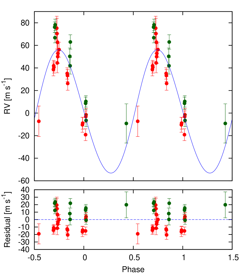
Figure 1.— Phased radial velocities for Kepler-91 in the absence of radial-velocity trend $\dot{\gamma}$. The data in 2013 and 2014 are shown by green and red points, respectively. The solid line is the best-fit radial-velocity curve to the data obtained by global modeling of photometric and radial-velocity data without considering $\dot{\gamma}$.

The binned light curve of Kepler-91 in Figure 2 shows a clear pattern of phase-curve variation; the double peaks at $\phi\sim 0.25$ and 0.75 are representative of the ellipsoidal variation. In addition, Figure 2 suggests a possible detection of secondary eclipse at $\phi\sim 0.5$, which means the reflected/emitted light from the planet is visible in the folded light curve. Therefore, following Jackson et al. (2012) and Hirano et al. (2015), we model the planet’s light $F_{p}$ by the following expression:

$$F_{p}=F_{0}-F_{1}\left(\frac{1+e\cos f}{1-e\sin\omega}\right)^{2}\sin(f+\omega-2\pi\Delta\phi),$$ (3)

where $F_{1}$ is the flux variation amplitude of planet’s reflected/emitted light and $F_{0}$ is the planetary flux offset arising from the homogeneous surface emission. Following Demory et al. (2013), Esteves et al. (2014), and Faigler & Mazeh (2014), we here introduce the “phase-delay” $\Delta\phi$ of the brightest part on the planet surface from the substellar point. The planetary light $F_{p}$ is added to the flux model for the beaming and ellipsoidal variation, integrated over the stellar visible hemisphere and wavelength through the Kepler band. In integrating the local flux calculated from the EVIL-MC model, we assume that the stellar effective temperature is 4550 K, and adopt the gravity darkening exponent of $\beta=0.093$ for Equation (10) of Jackson et al. (2012) based on the theoretical calculation by Claret (1998). The free parameters relevant to the light curve model are $a/R_{\star}$, the transit impact parameter $b$, limb-darkening coefficients $u_{1}+u_{2}$ and $u_{1}-u_{2}$ for the quadratic limb-darkening law, $q$ ($=M_{p}/M_{\star}$), $F_{0}$, $F_{1}$, $\Delta\phi$, the overall normalization factor $C$ for the folded light curve, $R_{p}/R_{\star}$, $e\cos\omega$, $e\sin\omega$, and $\Delta T_{c}$, which represents the small time deviation of the transit center from the ephemeris reported by the Kepler team. In our updated ephemeris, the initial transit center becomes $T_{c}^{(0)}-\Delta T_{c}$. We fix the orbital period to be $P_{\mathrm{orb}}=6.24668005$ d that are derived by the Kepler team based on the Q1–Q16 data (see section 4.1).

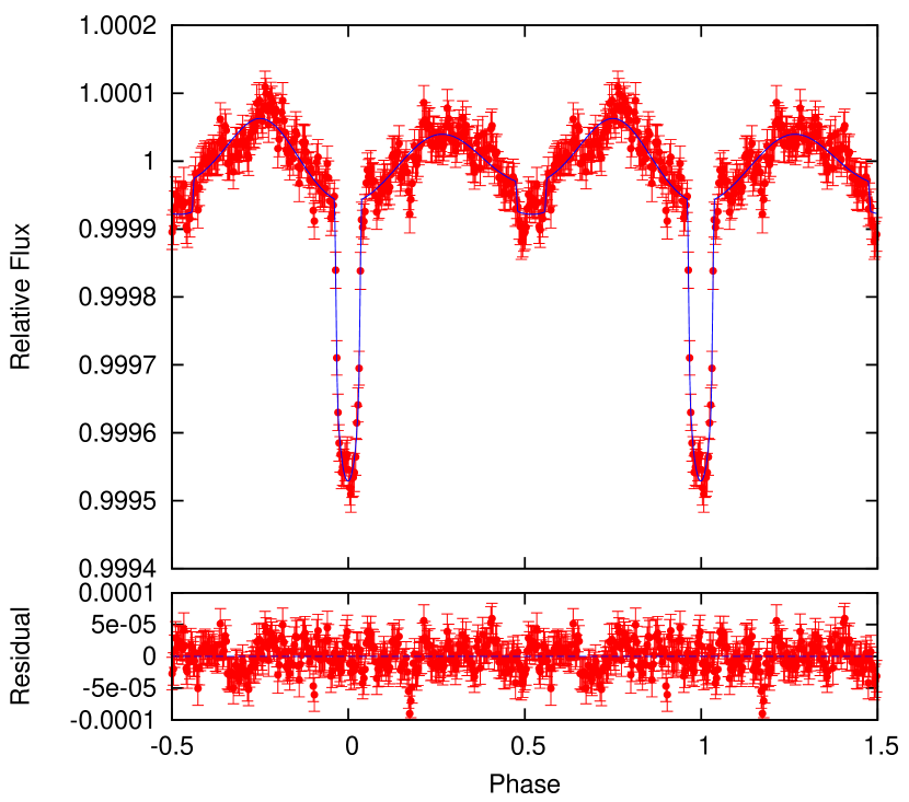
Figure 2.— Phased light curve for Kepler-91 (red points). The solid line is the best-fit light-curve model to the data obtained by global modeling of photometric and radial-velocity data considering the velocity trend ($\dot{\gamma}=-0.0612$ m s^-1day^-1).

Assuming that the likelihood is proportional to $\exp(-\chi^{2}/2)$ in Equation (1), we simultaneously model the observed radial velocity and light curve, and compute the posterior distribution for each fitting parameter by implementing Markov Chain Monte Carlo (MCMC) simulation. In addition to the above mentioned twelve parameters, we add $\gamma$ in Equation (2) to the fitting parameters. Note that the radial velocity semi-amplitude $K$ in Equation (2) is related to the planet-to-star mass ratio $q$ by

$$K=212908.30\left(\frac{M_{\star}/M_{\odot}}{P_{\mathrm{orb}}/\mathrm{day}}\right)^{\frac{1}{3}}\frac{q}{(1+q)^{\frac{2}{3}}}\frac{\sin i_{o}}{\sqrt{1-e^{2}}}~{}~{}~{}~{}(\mathrm{m~{}s}^{-1}).$$ (4)

In computing the posteriors, we do not impose priors on the fitting parameters except for $u_{1}$ and $u_{2}$; due to the sparse sampling of the long-cadence data ($\sim 30$ minutes) and quality of the binned light curve, the limb-darkening coefficients are poorly constrained in the absence of priors, and thus we decide to put Gaussian priors on the limb-darkening coefficients based on the theoretical table by Claret & Bloemen (2011) as $u_{1}+u_{2}=0.74\pm 0.01$ and $u_{1}-u_{2}=0.49\pm 0.01$. In our MCMC algorithm, originally developed in Hirano et al. (2012), the step size of each fitting parameter is iteratively scaled so that the overall acceptance ratio falls between 15% and 35% . After running 1,000,000 chains, the best-fit value and uncertainty for each fitting parameter are estimated from the median, and 15.87 and 84.13 percentiles of the marginalized posterior distribution of that parameter.

Shortly after we performed the first MCMC trial, we noticed a possible trend or drift in the observed radial velocities. Figure 1 plots the best-fit radial velocity curve as a function of the orbital phase $\phi$. For clarity, the data taken in 2013 are shown in green and those by the 2014 campaign are plotted in red. While we have detected a clear modulation with an amplitude of $\sim 50$ m s^-1, radial velocities take lower values for the 2014 data, which is evident in the bottom panel indicating the residual of the observed radial velocities from the best-fit model.

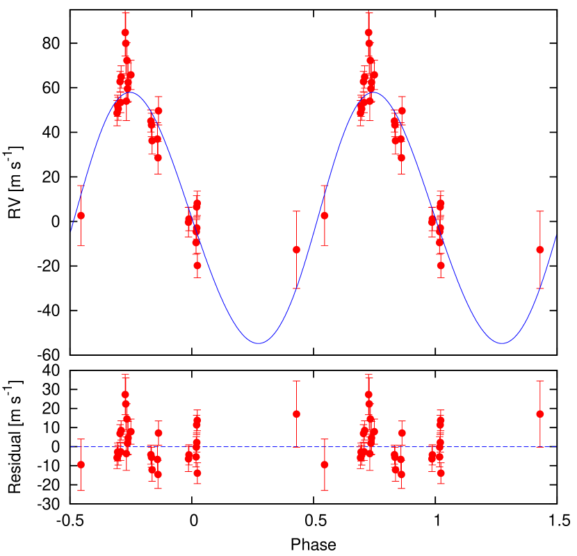
Figure 3.— Phased radial velocities for Kepler-91 (red points). The solid line is the best-fit radial-velocity curve to the data obtained by global modeling of photometric and radial-velocity data considering the velocity trend $\dot{\gamma}$. The derived $\dot{\gamma}$ ($=-0.0612$ m s^-1day^-1) was subtracted from the plot.

In order to confirm the presence of the radial velocity drift, we try to fit the data with an additional parameter: the radial velocity drift $\dot{\gamma}$. Adding the drift term $\dot{\gamma}\times t$ to the right side of Equation (2), we performed again the MCMC simulation to fit both radial velocity and light curve. The derived best-fit parameters and their uncertainties are summarized in Table 4. To compare between the radial velocity models with and without a drift term, we compute Bayesian Information Criteria (BIC) for the two cases, which is computed as $\mathrm{BIC}=\chi^{2}+n\ln(N_{\mathrm{data}})$, where $n$ is the number of free parameters and $N_{\mathrm{data}}$ is the number of data points. In the absence of a trend, we obtain $\mathrm{BIC}=477$, and for the case of the radial velocity model with $\dot{\gamma}$, BIC becomes 383; $\Delta\mathrm{BIC}$ is much larger than 10, meaning that the model with $\dot{\gamma}$ is strongly favored. Therefore, we conclude that a radial velocity drift (or trend) is present in our dataset, and report the best-fit parameters for the case with $\dot{\gamma}$ as the final result. We also tried several periods around $P_{\mathrm{orb}}$ and found that the $P_{\mathrm{orb}}-\sigma$ gave slightly better results in the global fitting than $P_{\mathrm{orb}}$ did ($\Delta{\chi^{2}}\simeq 7$). However, the resultant parameters for the two cases are well consistent within 0.2$\sigma$ level.

Figures 2 and 3 plot the folded light curve and radial velocities (red points) along with their best-fit models (blue line). The constant radial velocity offset and trend are both removed from the radial velocity data in Figure 3. The bottom panel in each figure shows the residuals from the best-fit model. From the posterior distribution of the fitting parameters, we also estimate the orbital and planetary parameters (e.g., the orbital inclination $i_{o}$, planet mass $M_{p}$ and radius $R_{p}$) assuming the stellar properties reported by asteroseismology (Table 1) to be $i_{o}=67.37^{+0.63}_{-0.65}$ deg, $M_{p}=0.66\pm 0.06~{}\mbox{M${}_{\rm Jup}$}$, and $R_{p}=1.40\pm 0.04~{}\mbox{R${}_{\rm Jup}$}$. These estimates are also shown in Table 4.

Table 4Orbital Parameters for Kepler-91

Parameter	Value (with trend)	Value (without trend)
$a/R_{\star}$	2.253${}^{+0.046}_{-0.045}$	2.238${}^{+0.046}_{-0.043}$
$b$	0.9041${}^{+0.0061}_{-0.0066}$	0.9062${}^{+0.0058}_{-0.0062}$
$u_{1}+u_{2}$	0.737${}^{+0.010}_{-0.0098}$	0.7370${}^{+0.0100}_{-0.0098}$
$u_{1}-u_{2}$	0.493${}^{+0.010}_{-0.010}$	0.493${}^{+0.0099}_{-0.010}$
$q(=M_{p}/M_{\star})$ (10-4)	4.82${}^{+0.19}_{-0.19}$	4.72${}^{+0.18}_{-0.18}$
$F_{0}$ (10-5)	5.65${}^{+0.57}_{-0.55}$	5.63${}^{+0.57}_{-0.58}$
$F_{1}$ (10-5)	1.41${}^{+0.30}_{-0.29}$	1.42${}^{+0.30}_{-0.28}$
$\Delta\phi$	0.394${}^{+0.029}_{-0.033}$	0.395${}^{+0.028}_{-0.032}$
$R_{p}/R_{\star}$	0.02286${}^{+0.00031}_{-0.00030}$	0.02294${}^{+0.00030}_{-0.00030}$
$e\cos\omega$	0.0280${}^{+0.0038}_{-0.0042}$	0.0277${}^{+0.0040}_{-0.0039}$
$e\sin\omega$	$-$0.043${}^{+0.011}_{-0.011}$	$-$0.046${}^{+0.011}_{-0.011}$
$\Delta T_{c}$ (10-3 day)	$-$1.09${}^{+0.34}_{-0.34}$	$-$1.11${}^{+0.34}_{-0.34}$
$\gamma$ (m s-1)	$-$42.5${}^{+2.0}_{-2.1}$	$-$33.2${}^{+1.8}_{-1.8}$
$\dot{\gamma}$ (m s-1 day-1)	$-$0.0612${}^{+0.0063}_{-0.0062}$	–
$\chi^{2}$	296	396
BIC	383	477
$i_{o}$ (deg)	67.37${}^{+0.63}_{-0.65}$	67.20${}^{+0.65}_{-0.66}$
$e$	0.0519${}^{+0.0095}_{-0.0088}$	0.0535${}^{+0.0099}_{-0.0091}$
$\omega$ (deg)	$-$57.2${}^{+8.7}_{-7.1}$	$-$58.8${}^{+8.4}_{-6.4}$
$M_{p}$ (MJup)	0.66$\pm$0.06	0.65$\pm$0.06
$R_{p}$ (RJup)	1.40$\pm$0.04	1.41$\pm$0.04

4.3. KOI-1894

The radial-velocity variations are less visible for KOI-1894 owing to the large radial-velocity error compared to the small semi-amplitude. The phase-folded light curve also shows a very tiny variation, if any, along the orbital phase. To extract possible planetary signals, we simultaneously model the radial velocities and light curve as in the case of Kepler-91. Since the observed transit depth and KOI-1894’s stellar radius suggest that the radius of the transiting companion (KOI-1894.01) is no more than $0.65R_{J}$, the reflected/emitted light from the planet is expected to be very small. According to Equations (1) – (3) in Shporer et al. (2011), the planetary reflection is estimated to be $\lesssim 1$ ppm at the location of KOI-1894.01, which is smaller than the expected amplitude of the ellipsoidal variation ($\sim 2$ ppm). Visual inspection of the binned light curve also suggests the absence of secondary eclipse. Thus for simplicity, we here neglect the planet flux $F_{p}$ for KOI-1894, and model the folded light curve with the ellipsoidal variation (including Doppler boosting) and transit only. Neglecting $F_{p}$ also helps to avoid $\chi^{2}$ being stuck at a local minimum during the optimization.

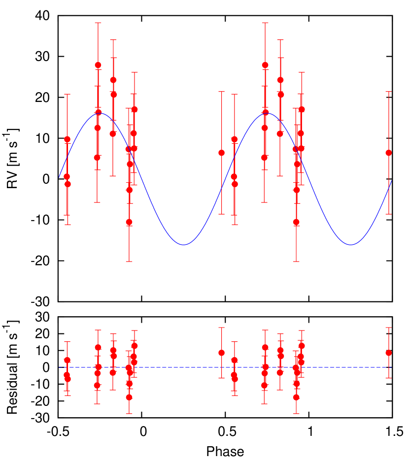
Figure 4.— Phased radial velocities for KOI-1894 (red points). The solid line is the best-fit radial-velocity curve to the data obtained by global modeling of photometric and radial-velocity data with the orbital eccentricity fixed to 0 and the stellar-density prior imposed.

Fixing the system parameters as $T_{\mathrm{eff}}=4992$ K, $M_{\star}=1.41M_{\odot}$, the gravity darkening exponent of $\beta=0.097$ (Claret, 1998), and $P_{\mathrm{orb}}=5.28789787~{}\mathrm{d}$ derived with the Q1–Q16 data (see section 4.1), we perform MCMC simulations for KOI-1894 to infer the posterior distributions for the fitting parameters. In the present case, we have the eleven free parameters: $a/R_{\star}$, $b$, $u_{1}+u_{2}$, $u_{1}-u_{2}$, $q$, $C$, $R_{p}/R_{\star}$, $e\cos\omega$, $e\sin\omega$, $\Delta T_{c}$, and $\gamma$. Again, we assume Gaussian priors for the limb-darkening parameters as $u_{1}+u_{2}=0.72\pm 0.01$, and $u_{1}-u_{2}=0.39\pm 0.01$ from the table by Claret & Bloemen (2011). Due to the weak radial-velocity signal of KOI-1894.01, we found that the global fit to the radial velocities and light curve exhibits a degeneracy between the fitting parameters (e.g., $a/R_{\star}$ and $q$). Thus, for KOI-1894, we also impose an additional prior on the host star’s density from Table 1 ($\rho_{\star}=(0.0259\pm 0.0055)\rho_{\odot}$), assuming a Gaussian distribution (Seager & Mallén-Ornelas, 2003). Otherwise, the fitting algorithm is exactly the same as for Kepler-91. The result of the fit is summarized in Table 5. The best-fit value for the mass ratio is $q=(1.02^{+0.44}_{-0.49})\times 10^{-4}$, implying $\sim 2\sigma$ detection of the planet. The mass and radius ratios are translated as $M_{p}=0.15^{+0.07}_{-0.08}~{}\mbox{M${}_{\rm Jup}$}$ and $R_{p}=0.64^{+0.04}_{-0.03}~{}\mbox{R${}_{\rm Jup}$}$ assuming the stellar mass and radius in Table 1. Table 5 also shows the result of our fit in the absence of the Gaussian prior on $\rho_{\star}$. As expected, the mass constraint is slightly weaker for this case.

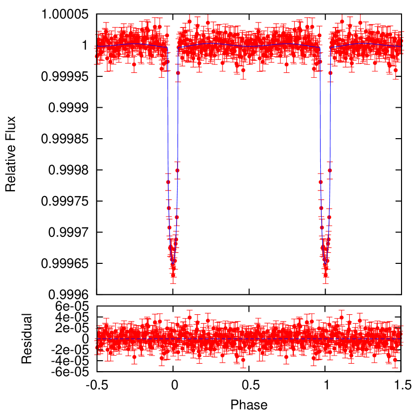
Figure 5.— Phased light curve for KOI-1894 (red points). The solid line is the best-fit light-curve model to the data obtained by global modeling of photometric and radial-velocity data with the orbital eccentricity fixed to 0 and the stellar-density prior imposed.

The orbital eccentricity is poorly constrained due to the small planetary signal and small number of radial velocity data, but we can rule out a high eccentricity ($e\gtrsim 0.25$) with our current datasets. We also try to fit the data with a circular orbit ($e=0$), and compare between the eccentric and circular cases. As shown in Table 5, the circular orbital fit yields a slightly better constraint on the mass ratio; $q=(1.19_{-0.41}^{+0.43})\times 10^{-4}$ with the stellar-density prior, leading to a $\sim 2.9\sigma$ detection. The mass and radius ratios are translated as $M_{p}=0.18\pm 0.07~{}\mbox{M${}_{\rm Jup}$}$ and $R_{p}=0.66\pm 0.04~{}\mbox{R${}_{\rm Jup}$}$ assuming the stellar mass and radius. Based on the $\chi^{2}$ values for the best-fit parameters, we compare BIC values for the two cases; BIC values of $295$ and $285$ are obtained for the eccentric and circular cases (with the stellar-density prior), respectively, so that fitting with a circular orbit is favored. The observed radial velocities and whole light curve are plotted in Figures 4 and 5, with their best-fit models for $e=0$. We also show zoomed-in versions of the transit and phase-curve variation in Figures 6 and 7, respectively. In Figure 7, the binned flux data used for the fit (250 bins) are plotted by the red crosses, and black points with errorbars indicate the flux data binned into 30 bins. We also tested several periods around $P_{\mathrm{orb}}$ and found that about $P_{\mathrm{orb}}-4\sigma$ gave the minimum $\chi^{2}$ value in the global fitting ($\chi^{2}\sim 200$), suggesting that the true period might exist around it. Nonetheless, the resultant parameters are well consistent with those for the case of $P_{\mathrm{orb}}$ within 0.2$\sigma$ level.

Our global analysis indicates the detection of KOI-1894.01 is still marginal, with only $\sim 2-3\sigma$ level, and the planet mass seems to be mainly constrained by the radial velocity data. In order to see if an independent estimate for the planet mass from the light curve alone gives a comparable result, we fit the folded light curve and estimate system parameters without radial velocity data. As a result, we obtain $q=(1.27_{-0.62}^{+0.71})\times 10^{-4}$, consistent with the above result by the global fit.

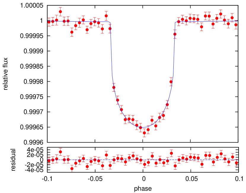
Figure 6.— Phased light curve for KOI-1894, zoomed in to show transit. The points and line are the same as those in figure 5.

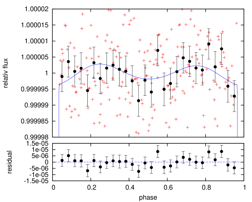
Figure 7.— Phase-folded light curve for KOI-1894, zoomed in to show the flux modulation by ellipsoidal variation. The red crosses are binned flux data used for the fit and black points with errorbars are data binned into 30 bins. The solid line is the same as that in figure 5.

5. Discussion and Summary

We reported the results of high-precision radial-velocity measurements with Subaru/HDS for the two Kepler evolved stars Kepler-91 and KOI-1894, which are candidates to host transiting planets.

Based on the simultaneous modeling of the radial-velocity data and Kepler light curves, we independently confirmed the planetary nature of Kepler-91b. The radial velocity semi-amplitude of $\sim 55$ m s^-1 we derived is consistent with what Barclay et al. (2014) found ($K=67\pm 11$ m s^-1) with $\sim 1\sigma$, but incompatible with the result by Lillo-Box et al. (2014b) who reported $K=93\pm 17$ m s^-1 with $\gtrsim 2\sigma$, although the reason for this discrepancy is unknown. We newly detected a drift of $\sim 20$ m s^-1 between the radial velocities taken at $\sim$ 1-yr interval thanks to our better measurement precision and longer period of time of observations compared to the previous ones. The persistent radial velocity drift is suggestive of a possible presence of another companion (planet) outside of Kepler-91b. Due to the lack of data, however, we are not able to pin down the period nor mass of the companion. Intensive high-precision radial-velocity monitoring of the star will uncover the unseen companion and provide hints for formation and evolution of the planetary system.

The estimated parameters for Kepler-91b in Table 4 are reasonably in good agreement with the previous study by Lillo-Box et al. (2014a, b) except for the mass ratio $q$ and scaled semi-major axis $a/R_{\star}$. This is likely because our radial velocity data show a smaller amplitude and planet mass is estimated to be small. Since the flux amplitude due to ellipsoidal variation is approximately proportional to $q(a/R_{\star})^{-3}$ (Shporer et al., 2011), a small $q$ resulted in the smaller $a/R_{\star}$ in order to explain the observed flux amplitude.

The westward phase-shift ($\Delta\phi>0$) of the flux maximum in planetary light (from the substellar point) is indicative of the inhomogeneous cloud coverage on the planetary surface. This is consistent with the trend that Esteves et al. (2014) found, claiming that westward phase-shifts are preferentially seen for relatively cool close-in planets with equilibrium temperatures of $T_{\rm eq}\lesssim 2500$ K; Lillo-Box et al. (2014a) estimated the equilibrium temperature of Kepler-91b to be $\sim 1920-2460$ K, depending on the assumed heat redistribution parameter. The magnitude of the phase-shift ($>0.35$) is, however, unusually large in our best-fit model compared with the previously reported values for other close-in planets (Lillo-Box et al., 2014a). The reason is unknown, but the huge coverage of the planet surface illuminated by the host star might be responsible. Note that we also detected a dip in the folded light curve (Figure 2) around $\phi=0.7$ reported in Lillo-Box et al. (2014a), and this dip should have more or less affected the fitting result.

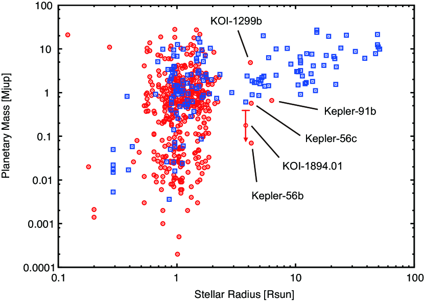
Figure 8.— Planetary mass plotted against host star’s radius. Red circles and blue squares represent true mass and projected mass, respectively. Planetary and stellar data were downloaded from NASA Exoplanet Archive, and only systems whose stellar mass and radius are both reported are plotted. Median and 3$\sigma$ upper limit value are shown for mass of KOI-1894.01.

Table 5Orbital Parameters for KOI-1894

Parameter	Value
	$e=0$ with $\rho_{\star}$ prior	$e$ free with $\rho_{\star}$ prior	$e=0$ without $\rho_{\star}$ prior	$e$ free without $\rho_{\star}$ prior
$a/R_{\star}$	3.79${}^{+0.24}_{-0.26}$	3.68${}^{+0.27}_{-0.31}$	4.25${}^{+0.37}_{-0.60}$	3.24${}^{+0.49}_{-0.57}$
$b$	0.634${}^{+0.065}_{-0.073}$	0.56${}^{+0.12}_{-0.10}$	0.48${}^{+0.19}_{-0.21}$	0.68${}^{+0.12}_{-0.095}$
$u_{1}+u_{2}$	0.724${}^{+0.0099}_{-0.010}$	0.723${}^{+0.011}_{-0.0098}$	0.724${}^{+0.010}_{-0.010}$	0.7271${}^{+0.0079}_{-0.0096}$
$u_{1}-u_{2}$	0.391${}^{+0.0098}_{-0.010}$	0.3908${}^{+0.0097}_{-0.0097}$	0.392${}^{+0.010}_{-0.0099}$	0.391${}^{+0.010}_{-0.0096}$
$q(=M_{p}/M_{\star})$ (10-4)	1.19${}^{+0.43}_{-0.41}$	1.02${}^{+0.44}_{-0.49}$	1.29${}^{+0.50}_{-0.51}$	0.70${}^{+0.47}_{-0.40}$
$F_{0}$ (10-5)	0 (fixed)	0 (fixed)	0 (fixed)	0 (fixed)
$F_{1}$ (10-5)	0 (fixed)	0 (fixed)	0 (fixed)	0 (fixed)
$\Delta\phi$	0 (fixed)	0 (fixed)	0 (fixed)	0 (fixed)
$R_{p}/R_{\star}$	0.01777${}^{+0.00041}_{-0.00035}$	0.01739${}^{+0.00063}_{-0.00035}$	0.01717${}^{+0.00081}_{-0.00042}$	0.01790${}^{+0.0010}_{-0.00046}$
$e\cos\omega$	0 (fixed)	0.052${}^{+0.12}_{-0.077}$	0 (fixed)	0.047${}^{+0.11}_{-0.23}$
$e\sin\omega$	0 (fixed)	0.085${}^{+0.086}_{-0.095}$	0 (fixed)	0.10${}^{+0.14}_{-0.13}$
$\Delta T_{c}$ (10-3 day)	$-$0.25${}^{+0.25}_{-0.40}$	$-$0.53${}^{+0.51}_{-0.79}$	$-$0.24${}^{+0.25}_{-0.41}$	$-$0.57${}^{+2.0}_{-1.0}$
$\gamma$ (m s-1)	$-$10.6${}^{+4.1}_{-4.1}$	$-$10.0${}^{+4.8}_{-3.9}$	$-$11.3${}^{+4.8}_{-4.7}$	$-$6.8${}^{+3.7}_{-4.9}$
$\chi^{2}$	234	233	235	233
BIC	285	295	286	294
$i_{o}$ (deg)	80.4${}^{+1.6}_{-1.8}$	80.2${}^{+2.1}_{-2.6}$	83.5${}^{+3.1}_{-4.1}$	76.2${}^{+4.0}_{-10.1}$
$e$	0 (fixed)	0.149${}^{+0.088}_{-0.077}$	0 (fixed)	0.186${}^{+0.15}_{-0.097}$
$\omega$ (deg)	0 (fixed)	61${}^{+45}_{-61}$	0 (fixed)	65${}^{+74}_{-70}$
$M_{p}$ (MJup)	0.18$\pm$0.07	0.15${}^{+0.07}_{-0.08}$	0.19$\pm$0.08	0.10${}^{+0.07}_{-0.06}$
$R_{p}$ (RJup)	0.66$\pm$0.04	0.64${}^{+0.04}_{-0.03}$	0.63$\pm 0.04$	0.66${}^{+0.05}_{-0.04}$

As for KOI-1894, we did not detect any statistically significant radial-velocity variations with our measurement precision of  9–15 m s^-1 and the number of data points. We excluded the possibility of a grazing transit by a binary companion for the star and set an upper limit on the mass of KOI-1894.01 to be $0.39~{}\mbox{M${}_{\rm Jup}$}$ by our non-detection of radial-velocity variations with 3$\sigma$ level. However, we detected possible radial-velocity variations with a semi-amplitude of $\sim$15 m s^-1 in phase with ellipsoidal variations of the star with 2–3$\sigma$ level. Although we can not say the detection is statistically significant at this stage, it suggests that the KOI-1894.01 could be a sub-saturn-mass planet. Figure 8 shows distribution of mass of exoplanets currently known plotted against their host star’s radius. As seen in the figure, KOI-1894.01 could be one of the lowest mass planets ever discovered around evolved stars together with Kepler-56b, a super-neptune-mass planet ($M_{p}=0.07~{}\mbox{M${}_{\rm Jup}$}$) detected via TTV (transit timing variation) method (Huber et al., 2013b). Actually the stellar parameters for KOI-1891 are similar to those of Kepler-56 (Huber et al., 2013a, $M_{\star}=1.32~{}\mbox{M${}_{\odot}$}$, $R_{\star}=4.23~{}\mbox{R${}_{\odot}$}$). Confirmation of KOI-1894.01 is highly encouraged in order to uncover such a new population of sub-saturn and super-neptune planets around relatively massive evolved stars, which have rarely been found so far either by radial-velocity surveys or transit ones.

References

- Barclay et al. (2014) Barclay, T. et al. 2014, ApJ, submitted (arXiv:1408.3149)
- Batalha et al. (2013) Batalha, N.M., et al. 2013, ApJS, 204, 24
- Butler et al. (1996) Butler, R. P., Marcy, G. W., Williams, E., McCarthy, C., Dosanjh, P., & Vogt, S. S. 1996, PASP, 108, 500
- Claret (1998) Claret, A. 1998, A&AS, 131, 395
- Claret & Bloemen (2011) Claret, A., & Bloemen, S. 2011, A&A, 529, A75
- da Silva et al. (2006) da Silva, L., et al. 2006, A&A, 458, 609
- Demory et al. (2013) Demory, B.-O., et al. 2013, ApJ, 776, L25
- Esteves et al. (2013) Esteves, L.J., De Mooij, E.J.W., & Jayawardhana, R. 2013, ApJ, 772, 51
- Esteves et al. (2014) Esteves, L. J., De Mooij, E. J. W., & Jayawardhana, R. 2014, ApJ, submitted (arXiv:1407.2245)
- Faigler & Mazeh (2011) Faigler, S., & Mazeh, T. 2011, MNRAS, 415, 3921
- Faigler & Mazeh (2014) Faigler, S., & Mazeh, T. 2014, ApJ, submitted (arXiv:1407.2361)
- Hirano et al. (2011) Hirano, T., Narita, N., Shporer, A., Sato, B., Aoki, W., & Tamura, M. 2011, PASJ, 63, 531
- Hirano et al. (2012) Hirano, T., et al. 2012, ApJ, 759, L36
- Hirano et al. (2015) Hirano, T., et al. 2015, ApJ, 799, 9
- Huber et al. (2013a) Huber, D. et al. 2013a, ApJ, 767, 127
- Huber et al. (2013b) Huber, D. et al. 2013b, Science, 342, 331
- Jackson et al. (2012) Jackson, B. K., Lewis, N. K., Barnes, J. W., Drake Deming, L., Showman, A. P., & Fortney, J. J. 2012, ApJ, 751, 112
- Johnson et al. (2007) Johnson, J.A., et al. 2007, ApJ, 665, 785
- Jones et al. (2014) Jones, M.I., Jenkins, J.S., Bluhm, P., Rojo, P., & Melo, C.H.F. 2014, A&A, 566, 113
- Kambe et al. (2002) Kambe, E., et al. 2002, PASJ, 54, 865
- Law et al. (2014) Law, N.M. et al. 2014, ApJ, 791, 35
- Lillo-Box et al. (2014a) Lillo-Box, J. et al. 2014a, A&A, 562, 109
- Lillo-Box et al. (2014b) Lillo-Box, J. et al. 2014b, A&A, 568, 1
- Liu et al. (2010) Liu, Y., Sato, B., Takeda, Y., Ando, H., & Zhao, G. 2010, PASJ, 62, 1071
- Mazeh et al. (2012) Mazeh, T., Nachmani, G., Sokol, G., Faigler, S., & Zucker, S. 2012, A&A, 541, A56
- Noguchi et al. (2002) Noguchi, K. et al. 2002, PASJ, 54, 855
- Ohta et al. (2009) Ohta, Y., Taruya, A., & Suto, Y. 2009, ApJ, 690, 1
- Sato et al. (2002) Sato, B., Kambe, E., Takeda, Y., Izumiura, H., & Ando, H. 2002, PASJ, 54, 873
- Sato et al. (2008) Sato, B., et al. 2008, PASJ, 60, 539
- Sato et al. (2012) Sato, B., et al. 2012, PASJ, 64, 97
- Sato et al. (2013) Sato, B., et al. 2013, PASJ, 65, 85
- Seager & Mallén-Ornelas (2003) Seager, S. & Mallén-Ornelas, G. 2003, ApJ, 585, 1038
- Seager & Deming (2010) Seager, S. & Deming, D. 2010, ARA&A, 48, 631
- Shporer et al. (2011) Shporer, A., et al. 2011, AJ, 142, 195
- Sliski & Kipping (2014) Sliski, D. H. & Kipping, D.M. 2014, ApJ, 788, 148
- Tajitsu et al. (2012) Tajitsu, A., Aoki, W, & Yamamuro, T, 2012, PASJ, 64, 77
- Takeda et al. (2008) Takeda, Y., Sato, B., & Murata, D., 2008, PASJ, 60, 781
- Valenti et al. (1995) Valenti, J. A., Butler, R. P. & Marcy, G. W. 1995, PASP, 107, 966.
- Wang et al. (2011) Wang, L., Liu, Y., Zhao, G., & Sato, B. 2011, PASJ, 63, 1035
- Winn (2011) Winn, J. N. 2011, in Exoplanets, ed. S. Seager (Tucson, AZ: University of Arizona Press), p.55–77
- Zielinski et al. (2012) Zielinski, P., Niedzielski, A., Wolszczan, A., Admow, M., & Nowak, G. 2012, A&A, 547, 91