Kinetics of Fluid Phase Separation

Abstract

We review understanding of kinetics of fluid phase separation in various space dimensions. Morphological differences, percolating or disconnected, based on overall composition in a binary liquid or density in a vapor-liquid system, have been pointed out. Depending upon the morphology, various possible mechanisms and corresponding theoretical predictions for domain growth are discussed. On computational front, useful models and simulation methodologies have been presented. Theoretically predicted growth laws have been tested via molecular dynamics simulations of vapor-liquid transitions. In case of disconnected structure, the mechanism has been confirmed directly. This is a brief review on the topic for a special issue on coarsening dynamics, expected to appear in Comptes Rendus Physique.

I Introduction

Topics related to phase transitions received significant attention over many decades MFisher1 ; HEStanley ; REvans ; KBinder1 ; KBinder2 ; DKashchiev ; RALJones1 ; AOnuki ; AJBray ; SPuri1 ; SKDas1 . The objective of this review is to discuss developments in the understanding of kinetics of phase transitions MFisher1 ; HEStanley ; REvans ; KBinder1 ; KBinder2 ; DKashchiev ; RALJones1 ; AOnuki ; AJBray ; SPuri1 ; SKDas1 ; IMLifshitz ; DAHuse1 ; JFMarko ; DWHeermann ; JVinals ; SMajumder1 ; SMajumder2 ; TBlanchard ; KBinder3 ; KBinder4 ; EDSiggia ; HFurukawa1 ; HFurukawa2 ; MSMiguel ; HTanaka1 ; HTanaka2 ; HTanaka3 ; FPerrot ; JPDelville ; JHobley ; DBeysens ; STanaka ; VMKendon ; SPuri2 ; CDatt ; MLaradji ; AKThakre ; SAhmad1 ; SAhmad2 ; SAhmad3 ; SKDas2 ; HKabrede ; SMajumder3 ; SRoy1 ; SRoy2 ; SRoy3 , with emphasis on phase separating fluid systems KBinder3 ; KBinder4 ; EDSiggia ; HFurukawa1 ; HFurukawa2 ; MSMiguel ; HTanaka1 ; HTanaka2 ; HTanaka3 ; FPerrot ; JPDelville ; JHobley ; DBeysens ; STanaka ; VMKendon ; SPuri2 ; CDatt ; MLaradji ; AKThakre ; SAhmad1 ; SAhmad2 ; SAhmad3 ; SKDas2 ; HKabrede ; SMajumder3 ; SRoy1 ; SRoy2 ; SRoy3 ; SWKoch ; JMidya . Evolution of a system from one equilibrium phase to another is a nonequilibrium phenomenon and happens via nucleation MFisher1 ; HEStanley ; REvans ; KBinder1 ; KBinder2 ; DKashchiev and growth KBinder2 ; RALJones1 ; AOnuki ; AJBray ; SPuri1 ; SKDas1 of domains. E.g., when a homogeneous binary mixture ($A+B$), liquid or solid, is quenched inside the miscibility gap, it becomes unstable to fluctuations and moves towards the coexisting phase-separated state via formation and growth of domains rich in $A$ and $B$ particles. For a vapor-liquid transition, the approach to the new equilibrium occurs via formation of particle rich and particle poor regions.

Typically, the growth of domains is a scaling phenomena AJBray , i.e., there is self-similarity of patterns at two different times, despite a change in length scale $\ell(t)$, the average size of domains at time $t$. This is captured in the scaling properties AJBray

$$C(r,t)\equiv\tilde{C}[r/\ell(t)],$$ (1)

$$S(k,t)\equiv\ell(t)^{d}\tilde{S}[k\ell(t)],$$ (2)

$$P(\ell_{d},t)\equiv\ell(t)^{-1}\tilde{P}[\ell_{d}/\ell(t)],$$ (3)

of the two-point equal time correlation function ($C$), structure factor ($S$) and domain size distribution function ($P$). In Eqs. (1-3), $r$ is the distance between two points ($\vec{r_{i}}$ and $\vec{r_{j}}$), $k$ is the wave vector, $\ell_{d}$ is the size of a domain and $d$ is the system dimensionality. There $\tilde{C}$($x$), $\tilde{S}$($y$) and $\tilde{P}$($z$) are master functions, independent of time. The above mentioned correlation function is calculated as AJBray

$$C(r,t)=<\psi(\vec{r_{i}},t)\psi(\vec{r_{j}},t)>-<\psi(\vec{r_{i}},t)><\psi(\vec{r_{j}},t)>,$$ (4)

where $\psi$ is the relevant order-parameter for the transition. $S(k,t)$ is the Fourier transform of $C(r,t)$. The scalar notations $r$ and $k$ imply spherical isotropy and are applicable for systems without any bias such that the structures are isotropic in statistical sense. The angular brackets in Eq.(4) are for statistical averaging.

Typically, $\ell(t)$ grows with time in power-law fashion as AJBray

$$\ell(t)\sim t^{\alpha}.$$ (5)

The growth exponent $\alpha$ depends upon $d$, number of order-parameter components, morphology, hydrodynamic effects and conservation of order-parameter AJBray . In out of equilibrium systems, as is clear from Eq. (4), the order parameter $\psi$ is a function of space and time. In a magnetic system this can be identified with the local magnetization, in a binary mixture with the local difference between the concentration of the two species, for a vapor-liquid system with the density. Depending upon the type of transition, the total order-parameter (the local value integrated over the whole system) may or may not remain same at all times. E.g., in a paramagnetic to ferromagnetic transition, where, starting from a zero net magnetization, the system gets spontaneously magnetized, the order-parameter is a nonconserved quantity. On the other hand, for all types of phase separating systems, assuming that there is no chemical conversion or flow of material between the system and a reservoir, this is a conserved quantity. In this paper we will deal with conserved scalar order parameter.

Major fraction of the literature in kinetics of phase transitions is related to the behavior of $C(r,t)$ and understanding of the exponent $\alpha$. However, there exist other interesting aspects, e.g., aging DSFisher1 and persistence SNMajumdar . In aging phenomena, typically one studies the two-time quantities, e.g., the order-parameter autocorrelation function DSFisher1

$$C_{\rm{age}}(t,t_{w})=<\psi(\vec{r_{i}},t)\psi(\vec{r_{i}},t_{w})>-<\psi(\vec{r_{i}},t)><\psi(\vec{r_{i}},t_{w})>,$$ (6)

where $t_{w}$ and $t$ ($>t_{w}$) are respectively the waiting and observation times. Even though the time translation invariance is not obeyed by $C_{\rm{age}}(t,t_{w})$ in out of equilibrium systems, this quantity is expected to exhibit scaling DSFisher1 with respect to $t/t_{w}$. An objective in studies related to aging is to obtain scaling functions for $C_{\rm{age}}$ or for other two-time quantities of relevance, in different types of phase transitions. Persistence, on the other hand, is related to the time dependence of the fraction of unaffected local order parameter.

Each of these aspects are better understood in nonconserved order-parameter case AJBray . For conserved order-parameter, significant progress has been made only with respect to the growth exponent $\alpha$, for solid binary mixtures IMLifshitz ; DAHuse1 ; JFMarko ; DWHeermann ; JVinals ; SMajumder1 ; SMajumder2 . For the latter, diffusion (via evaporation and condensation) is the only transport mechanism and the growth is characterized by a single exponent. In fluids, however, no single exponent describes the entire growth process AJBray . This is due to the faster transport of material, particularly due to the influence of hydrodynamics, at late times. Effects of such fast transport may be manifested in different ways depending upon system dimensionality and domain pattern. Thus, kinetics of phase separation in fluids is a richer and challenging area. In spite of that, reasonable progress has been made KBinder3 ; KBinder4 ; EDSiggia ; HFurukawa1 ; HFurukawa2 ; MSMiguel ; HTanaka3 ; FPerrot ; JPDelville ; JHobley ; DBeysens ; STanaka ; VMKendon ; SPuri2 ; CDatt ; MLaradji ; AKThakre ; SAhmad1 ; SAhmad2 ; SAhmad3 ; SKDas2 ; HKabrede ; SMajumder3 ; SRoy1 ; SRoy2 ; SRoy3 ; SWKoch ; JMidya . The aim of the article is to review some of these works in brief.

The rest of the article is organized as follows. In section II we discuss the theoretical progress. Section III is devoted to the discussion of models and computational methods. Representative computational results are presented in section IV. Finally, section V concludes the paper with a brief summary and outlook.

II Theories

In a solid binary mixture, the rate of change of domain size is associated with the chemical potential gradient as DAHuse1 $d\ell/dt\sim|\vec{\nabla}\mu|$. Using the dimensionality of $\mu$ as $\gamma/\ell$, $\gamma$ being the interfacial tension and assuming that a gradient exists over the length of the domain size, one obtains DAHuse1

$$\frac{d\ell}{dt}\sim\frac{\gamma}{\ell^{2}}.$$ (7)

Solution of Eq.(7) provides $\alpha=1/3$, referred to as the Lifshitz-Slyozov (LS) law IMLifshitz and is understood to be valid for any domain growth occurring via simple diffusive mechanism.

Early part of fluid phase separation is also dominated by diffusion and thus, is expected to have $\alpha=1/3$. At late times, hydrodynamic effects become more important, for percolating domain morphology. As already mentioned, while for phase separation in solid mixtures system dimensionality and domain morphology do not play important role SMajumder2 , these become crucial for selection of mechanism in fluids. In some cases, different mechanisms may give rise to same value of the growth exponent. Thus, very direct computational or experimental probes are necessary to validate a particular one. Below we will discuss some relevant mechanisms briefly.

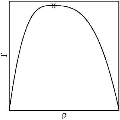
Figure 1: Schematic diagram for vapor-liquid coexistence in $T$ vs $\rho$ plane. The critical point is marked by a cross. The left and right branches represent respectively the vapor and the liquid densities. From Molecular simulation.

Typically, phase separating systems exhibit interconnected or droplet morphology, depending upon the overall composition or density of the system. In Fig.1 we show a vapor-liquid coexistence curve in temperature ($T$) versus density ($\rho$) plane. There the left branch corresponds to the vapor-phase density and the right one to the liquid-phase density. For a binary mixture phase separation, the appropriate abscissa variable is the concentration of one of the species. For density or composition very close to the coexistence curve (vapor branch in vapor-liquid transition), droplet like pattern is visible, from the very beginning. In this under-saturation case, the system requires fluctuations involving large length scales to nucleate stable droplets that can grow. Such events, depending upon the proximity to the coexistence curve, may be rare and the phase separation can be delayed. On the other hand, far from the coexistence curve, the system falls unstable to infinitesimal fluctuations and the corresponding phase separation process is referred to as the spinodal decomposition. Typically, in this case, the domain morphology is percolating. Here we caution the reader that at late time droplet structures can emerge from percolating morphology as well CDatt , if the system is away from the critical composition or density. In fluids this is expected to happen faster.

Let us first consider the case of percolating domain morphology. Because of experimental realizability, we will first take up the $d=3$ case. The hydrodynamic regime is divided into two subregimes AJBray , viz., viscous and inertial. These we discuss below, following Siggia EDSiggia and Furukawa HFurukawa1 ; HFurukawa2 , using the Navier-Stokes (NS) equation

$$\rho\frac{D}{Dt}\vec{v}-\nu\nabla^{2}\vec{v}=-\vec{\nabla}p.$$ (8)

In Eq.(8), $\rho$ is the mass density, $\vec{v}$ is the fluid velocity, $\nu$ is the kinematic viscosity, $p$ is the pressure and $D/Dt=d/dt+(\vec{v}.\vec{\nabla})$. In $D\vec{v}/Dt$, both the terms stand for acceleration, as can be checked dimensionally. The second one is related to convection where the acceleration is generated by space dependent velocity. Eq.(8) is essentially related to balancing of force coming from pressure with that of frictions. On the left hand side, the first term can be treated as inertial friction and the second one is related to dissipative friction originating from viscous drag. Via dimensional substitutions $Dv/Dt\equiv v/t$, $\nabla^{2}v\equiv-v/\ell^{2}$ and considering that the pressure gradient is obtainable from interfacial tension $\gamma$, one writes, after multiplying both sides by $vt$,

$$\rho v^{2}+\frac{\rho\nu}{\ell}v=\frac{\gamma}{\ell}.$$ (9)

The second term on the left hand side of Eq.(9) is related to the inverse of time dependent Reynolds number and is important at earlier part of the hydrodynamic regime, providing viscous growth. At later time, the first term dominates, giving rise to the inertial hydrodynamic growth. Thus, in the first part of hydrodynamic growth it is equivalent to equating the interfacial free energy density with the viscous stress and in the second part, the same with the kinetic energy density EDSiggia . With the understanding that there exist unique time and length scales in the problem, one identifies $v$ with $d\ell/dt$. Then, in the viscous regime one obtains

$$\frac{d\ell}{dt}=\frac{\gamma}{\rho\nu},$$ (10)

and in the inertial regime

$$\frac{d\ell}{dt}=\sqrt{\frac{\gamma}{\rho\ell}}.$$ (11)

Solutions of Eqs. (10) and (11) provide $\alpha=1$ and $2/3$, respectively.

Recall that our discussion is related to interconnected domain morphology, having tube-like structure in $d=3$. The fast advective transport of material through these tubes happens due to pressure gradient calculable from interfacial tension and domain size. In $d=2$, analogue of a tube is strip. San Miguel et al. MSMiguel argued that fluctuations along the linear boundaries of these strips significantly increase the interfacial free energy due to increase in curvature. This mechanism thus lacks instability. According to these authors, instead of a crossover from $\alpha=1/3$ to $1$, as in $d=3$, the $2-d$ fluid will encounter a crossover from $1/3$ to $1/2$, the latter coming from an interface diffusion mechanism MSMiguel . There a crossover from $\alpha=1/3$ to $1$ will require large fluctuations, may become possible only at very high temperatures. In the interface diffusion mechanism, break-up of strips into droplets is expected MSMiguel . In that case, droplet diffusion and collision mechanism of Binder and Stauffer (BS) KBinder3 ; KBinder4 ; EDSiggia , in general valid for off-critical fluid quenches, is expected to be operative. This we discuss below. Note that, in case of droplet morphology, the growth description cannot be provided via NS equation AJBray .

As opposed to solid binary mixtures, droplets in fluids are significantly mobile. This gives rise to, in addition to the standard evaporation-condensation process, another growth mechanism involving diffusion and collision of droplets. These are inelastic collisions, following which the colliding partners merge, forming a bigger droplet and reducing the droplet density ($n$). For the decay of $n$, one can write EDSiggia

$$\frac{dn}{dt}=KD_{\ell}\ell n^{2},$$ (12)

where $K$ is a constant and $D_{\ell}$ is the diffusion constant for a droplet of size $\ell$. Following Stokes-Einstein-Sutherland relation JPHansen , $D_{\ell}\ell$ can be treated as a constant. Using $n\sim 1/\ell^{d}$, one obtains EDSiggia

$$\frac{d\ell}{dt}\propto\frac{1}{\ell^{d-1}}.$$ (13)

Solution of Eq.(13) provides $\alpha=1/d$. Thus, in $d=2$, BS value of $\alpha$ is same as that for the interface diffusion mechanism of San Miguel et al. On the other hand, in $d=3$, BS mechanism provides a value of $\alpha$ coinciding with the LS value. It is expected that the amplitudes will be different for different mechanisms that provide same exponents. E.g., in $d=3$ LS mechanism should have a smaller amplitude than the BS one. Direct verification of the latter is possible via computer simulations SRoy1 . Tanaka HTanaka1 ; HTanaka2 ; HTanaka3 argued that in high droplet density situation, motion of the droplets will not be random due to inter-droplet interaction. However, incorporation of such fact merely changes the growth amplitude. Presence of such interaction can be verified by calculating the mean-squared-displacements (MSD) JPHansen of the droplets.

Pictures presented above are primarily meant for kinetics of incompressible liquid-liquid phase separation. Nevertheless, they may apply for vapor-liquid phase separation to a good extent. This, however, requires verification.

III Models and Methods

Kinetics of phase separation in solid binary mixtures at atomistic level have been traditionally studied via Monte Carlo (MC) simulations DPLandau of the nearest neighbor Ising model

$$H=-J\sum_{<ij>}S_{i}S_{j};~{}~{}J>0;~{}S_{i}=\pm 1,$$ (14)

on regular lattice. Here, an up spin ($S_{i}=+1$) corresponds to an $A$ particle and a down spin ($S_{i}=-1$) to a $B$ particle. In this model, the kinetics is introduced via the Kawasaki exchange DPLandau trial moves in which positions of two nearest neighbor particles are interchanged. These moves are accepted according to the standard Metropolis algorithm DPLandau . At the coarse-grained level, one solves the Cahn-Hilliard (CH) equation AJBray

$$\frac{\partial\psi(\vec{r},t)}{\partial t}=-\nabla^{2}\Big{[}\psi(\vec{r},t)+\nabla^{2}\psi(\vec{r},t)-\psi^{3}(\vec{r},t)\Big{]},$$ (15)

where the order-parameter $\psi$ can be thought of being obtained from the coarse-graining of the Ising spins over a length scale of the order of the equilibrium correlation length $\xi$. Thus, the CH equation provides an advantage of accessing large effective length scale within practically accessible computation time. Eq.(15) can one way be obtained from the Ising model via a master equation approach with Kawasaki kinetics as an input ISchmidt ; SKDas3 . Despite the latter being a direct and rigorous approach, in this article we will present a phenomenological derivation. Eq.(15) is solved on regular lattice, typically via Eular discretization technique SKDas3 . This model, according to the nomenclature of Hohenberg and Halperin MPAllen , is referred to as the model B.

In fluids, at coarse-grained level the kinetics is typically studied via model H MPAllen which is a combination of the CH and the NS equations, the latter taking care of the fluid flow. To describe this model, derivation of the CH equation AJBray will be of help. Recalling that we are dealing with conserved order-parameter, one writes the continuity equation

$$\frac{\partial\psi}{\partial t}=-\vec{\nabla}\cdot\vec{J_{c}},$$ (16)

where the current $\vec{J_{c}}$ comes from the gradient of the chemical potential $-\vec{\nabla}\mu$. The chemical potential can be obtained from the functional derivative as

$$\mu=\frac{\delta F[\psi(\vec{r},t)]}{\delta\psi(\vec{r},t)},$$ (17)

the free energy functional being the Ginzburg-Landau one

$$F=k_{B}T\int d\vec{r}[-a\psi^{2}+b\psi^{4}+c(\vec{\nabla}\psi)^{2}],$$ (18)

where the positive coefficients a, b, and c are temperature dependent. Often these coefficients are scaled in such a way that the final form is parameter free, as Eq.(15).

The model H equations read AJBray , in the incompressible limit ($\vec{\nabla}\cdot\vec{v}=0$), as

$$\frac{\partial\psi}{\partial t}+\vec{v}\cdot\vec{\nabla}\psi=\nabla^{2}\mu,$$ (19)

$$\rho\frac{D\vec{v}}{Dt}-\nu\nabla^{2}\vec{v}=-\vec{\nabla}p-\psi\vec{\nabla}\mu.$$ (20)

In addition to the pure CH and NS equations, there are additional terms in Eqs.(19) and (20), coming from the coupling between the velocity and order-parameter fields. This is justifiable, e.g., the current $\vec{J_{c}}$ in the CH equation is expected to be influenced by the velocity field, becoming

$$\vec{J_{c}}=-\vec{\nabla}\mu-\psi\vec{v},$$ (21)

and the chemical potential gradient should provide a driving force to affect the velocity field in the NS equation. Again, these equations can be solved on regular lattice. This model is very much phenomenological and a microscopic derivation like the CH equation ISchmidt is still lacking. Such an objective can possibly be achieved KKaski via the construction of free energy functionals by taking density and velocity distributions as inputs from molecular dynamics (MD) simulations at various coarse-grained levels, by appropriately adjusting the effective inter-particle potential at successive steps. A multi-scale method like this may seem obvious but has never been demonstrated. Success of the method may prove useful in justifying similar (elegant) phenomenological models in more complex problems like active matter SRamaswamy .

The incorporation of the coupled terms in Eqs. (19) and (20), in a sense, guarantee the simultaneous growth in the velocity and density fields. While such facts have been reported from Lattice Boltzmann simulations SPuri1 ; VMKendon , are lacking in MD simulations even though the latter is more direct and accurate. Thus, a microscopic justification of the model, particularly understanding of the importance of additional higher order terms, is needed.

As can be guessed from the above discussion, at atomistic level, kinetics of fluid phase separation is studied via MD simulations MPAllen ; DFrenkel ; DCRapaport in which hydrodynamics can be easily implemented. For this purpose, the interatomic interactions are popularly incorporated via the well known Lennard-Jones (LJ) potential

$$u(r)=4\varepsilon\Big{[}\Big{(}\frac{\sigma}{r}\Big{)}^{12}-\Big{(}\frac{\sigma}{r}\Big{)}^{6}\Big{]},$$ (22)

where $r$ ($=|\vec{r_{i}}-\vec{r_{j}}|$) is the distance between two particles at $\vec{r_{i}}$ and $\vec{r_{j}}$, $\varepsilon$ is the interaction strength and $\sigma$ is the interparticle diameter. In a binary (or multicomponent) mixture, $\varepsilon$ and $\sigma$ can be chosen to be different for different combinations of species.

In standard MD simulations, equations of motion are solved in discrete time, typically via Verlet velocity algorithm MPAllen ; DFrenkel . Conservation laws of hydrodynamics are perfectly satisfied in microcanonical ensemble using which various fluid transport properties are calculated in equilibrium. However, for kinetics of phase separation, following a temperature quench, in course of the system’s evolution, the potential energy decreases, for energy driven phase transitions. In a constant energy ensemble, thus, the kinetic energy, i.e., the temperature increases, destroying the objective of the study. Therefore, simulations in canonical ensemble, with appropriate hydrodynamics preserving thermostat, become essential. There are a number of good methods for this purpose, e.g., dissipative particle dynamics PNikumen ; SDStoyarnov ; CPastorino , multiparticle collision dynamics AWinkler , Lowe-Andersen thermostat EAKoopman , Nosé-Hoover thermostat DFrenkel , etc. In this article, presented results were obtained via application of the Nosé-Hoover thermostat (NHT) which will be discussed soon.

IV Simulation Results

Binary fluid phase separation has been extensively studied via lattice Boltzmann simulations or simpler solutions of the model H equations VMKendon ; SPuri2 ; CDatt , for critical quenches. Though MD simulations in this context are relatively rare, the theoretical expectations for critical quenches are confirmed to a good degree SKDas1 ; MLaradji ; AKThakre ; SAhmad1 ; SAhmad2 ; SAhmad3 and reviews are available. Here we focus on vapor-liquid phase separation, with particular emphasis on off-critical quenches, providing droplet morphology, for which MD simulations are mostly recent SKDas2 ; HKabrede ; SMajumder3 ; SRoy1 ; SRoy2 ; SRoy3 ; SWKoch ; JMidya .

All results were obtained via a modified LJ potential MPAllen

$$U(r<r_{c}) = u(r)-u(r_{c})-(r-r_{c})\frac{du(r)}{dr}\Big{|}_{r=r_{c}},$$

$$U(r\geq r_{c}) = 0.$$ (23)

The cut-off radius $r_{c}$ ($=2.5\sigma$) is introduced for a faster computation. Note that, in critical phenomena MFisher1 ; HEStanley , LJ potential being a short-range one, this does not alter the universality class. Due to the cut-off and shifting of the potential to $0$ at $r=r_{c}$, a discontinuity in the force is created which may cause non-smooth behavior in energy and thus may be problematic for energy and momentum conservations, necessary for preservation of hydrodynamics. This problem is corrected by incorporating the last term in the first part of Eq.(IV).

The phase diagram, the primary requirement before studying the kinetics of phase separation, for atomistic models can be obtained using both MC and MD simulations. As is well known, equilibrium phase behavior and thermodynamic properties are insensitive to ensemble and technicality related to transport mechanism. Thus, MC simulations with smart ensembles are advantageous, compared to MD. For vapor-liquid phase transition, typically one uses grandcanonical and “Gibbs” ensemble methods DPLandau . With grandcanonical ensemble, other thermodynamic properties, e.g., compressibility, can be easily obtained to study its critical singularity.

As mentioned, an NHT was applied to study dynamics via MD. There one solves the deterministic equations of motion DFrenkel

$$m\dot{\vec{r_{i}}}=\vec{p_{i}},$$ (24)

$$\dot{\vec{p_{i}}}=-\frac{\delta U}{\delta\vec{r_{i}}}-\Xi\vec{p_{i}},$$ (25)

$$\dot{\Xi}=\frac{\Big{[}\sum\limits_{i=1}^{N}(p_{i}^{2}/m)-3Nk_{B}T\Big{]}}{Q}.$$ (26)

In Eqs.(24-26), $m$ is the particle mass (set equal for all), $\Xi$ is a time dependent drag that adjusts its value depending upon the drift of temperature from the assigned value, $N$ is the number of particles, $k_{B}$ is the Boltzmann constant and $Q$ is the coupling strength between the system and the thermostat. Essentially, in this scheme one works with a microcanonical ensemble with a modified Hamiltonian. Results thus obtained are equivalent to those from the canonical ensemble with the original Hamiltonian DFrenkel ; SDStoyarnov .

There exist better hydrodynamics preserving thermostats. But for the present purpose, the NHT appears adequate. The results obtained using this thermostat have been tested against other methods. For example, in $d=2$, we have compared JMidya them with the Lowe-Andersen thermostat (LAT). The LAT is an improvement over the basic Andersen thermostat (AT). In the AT randomly chosen particles are assigned new velocities (with Maxwell distribution) to keep the temperature at a desired value and thus stochastic in nature, like MC methods. In the LAT, while assigning new velocities, conservation of local momentum is appropriately taken care of. Further, inside the coexistence region, transport properties of droplets (from equilibrium configuration), calculated via NHT, are found to be in good agreement with the calculations using microcanonical ensemble SRoy2 ; SRoy3 . Also, in a binary fluid, critical behavior of shear viscosity was nicely reproduced via NHT SRoy4 . In addition, from experience we feel that the NHT provides a superior control over temperature, compared to few other better hydrodynamics preserving thermostats, particularly in out-of-equilibrium situation.

We will present results SKDas2 ; HKabrede ; SMajumder3 ; SRoy1 ; SRoy2 ; SRoy3 ; SWKoch ; JMidya in both $d=2$ and $3$, from MD simulations in periodic square or cubic boxes of linear dimension $L$ (in units of $\sigma$). All results were obtained after averaging over adequately large numbers of independent initial configurations. In the solutions of the equations of motion we have used time discretization $\Delta t=0.005t_{0}$, $t_{0}$[$=(m\sigma^{2}/\varepsilon)^{1/2}$] being an LJ time unit. Note that the critical temperature and the critical number density for this model in $d=3$ respectively are $\simeq 0.9\varepsilon/k_{B}$ and $\simeq 0.3$. All results in $d=3$ correspond to quenches from $T=\infty$ to $0.6\epsilon/k_{B}$. As expected, the value of $T_{c}$ in $d=2$ is lower ($\simeq 0.5\varepsilon/k_{B}$). The quench temperature there is $0.25\varepsilon/k_{B}$.

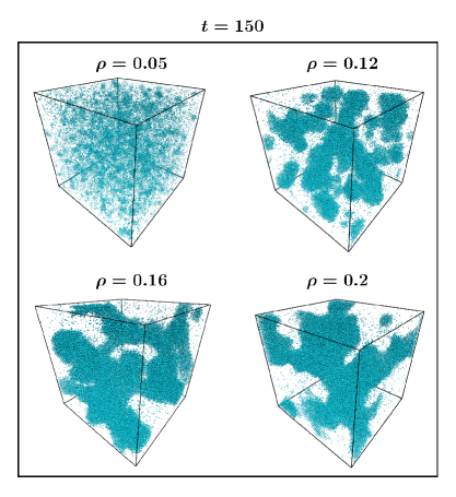
Figure 2: Evolution snapshots for various overall densities $\rho$, obtained from molecular dynamics simulations of the single component Lennard-Jones model in $d=3$. In all the cases the time, temperature and the system size were fixed to $t=150$, $T=0.6$ and $L=80$. From J. Chem. Phys. 139, 044911 (2013).

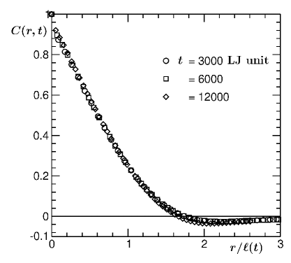
Figure 3: Scaling plot of $C(r,t)$ as a function of $r/\ell(t)$, for $\rho=0.05$. Data from few different times are included. The results correspond to droplet morphology in $d=3$. From Soft Matter 9, 4178 (2013).

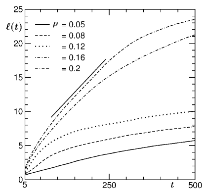
Figure 4: Plots of $\ell(t)$ versus $t$, for different values of $\rho$, in $d=3$. The continuous straight line corresponds to viscous hydrodynamics growth. From J. Chem. Phys. 139, 044911 (2013).

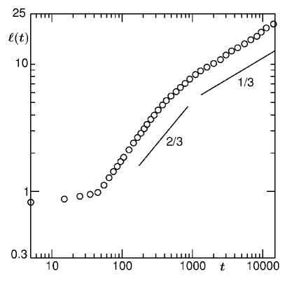
Figure 5: Log-log plot of $\ell$ versus $t$, for $\rho=0.05$, that corresponds to droplet morphology in $d=3$. The solid lines correspond to power-laws, exponents being mentioned on the figure. From Phys. Rev. E 85, 050602(R) (2012).

In Fig.2 we present snapshots from $d=3$ (unless otherwise mentioned, results are from this dimension) for different overall densities . It is clearly seen that as one approaches the vapor branch of the coexistence curve, the morphology becomes more droplet like. Given that we have access to both percolating and droplet structures, a wide variety of mechanisms can be checked.

In Fig.3 we show a scaling plot of the correlation functions for droplet morphology, using data from different times. For this calculation, the order parameter $\psi$ was given a value $+1$ if the density at a point is higher than the overall density $\rho$ and $-1$ otherwise. Nice collapse of data, versus $r/\ell(t)$, confirms self-similarity of structure. Note here that we have obtained $\ell(t)$ from different methods, from the lengths at which $C(r,t)$ decays to a particular value, from the first moment of $P(\ell_{d},t)$, as well as by identifying domain boundaries and directly counting the number of particles inside them. For the last method, cube (square in $d=2$) root of the average number of particles inside the liquid regions will provide $\ell(t)$. For the sake of brevity we present results only from the correlation functions.

In Fig.4 we show plots of $\ell(t)$ vs $t$, for various values of $\rho$. It appears that closer to the critical density there is a linear growth, after a brief slow regime, before hitting the finite-size effects. The slower part at the very beginning can be attributed to the LS behavior IMLifshitz and the linear one to the viscous hydrodynamic one EDSiggia ; HFurukawa1 ; HFurukawa2 . Due to the demanding nature of MD simulations, to the best of our knowledge, a crossover from viscous to inertial hydrodynamic regime is not yet appropriately observed, using this method. However, for intermediate densities, we observed a $t^{2/3}$ behavior even before a linear growth appears. This has been checked SRoy3 via appropriate finite-size scaling analysis MFisher2 which we do not present here. A possible reason for observing the exponent $2/3$ during early period of the hydrodynamic growth can be the following. In the inertial regime, due to the large mass of domains, there may be competition between growth and break-up. In intermediate density regime, where interconnectedness of the domain morphology is not very robust, the break-up becomes easier. For densities very close to the coexistence vapor density, certainly the growth is much slower. This we discuss in details below SRoy1 ; SRoy2 ; SRoy3 .

In Fig.5 we take a look at the results for $\rho=0.05$ on a double-log scale. The flat behavior of the data at the beginning is due to delayed nucleation. A very fast rise after this signals the onset of nucleation, following which the data are consistent with a $t^{1/3}$ growth. As mentioned already, in $d=3$ this behavior can be due to LS IMLifshitz ; DAHuse1 as well as BS KBinder3 ; KBinder4 ; EDSiggia mechanism. To select from the multiple possibilities we do the following exercise.

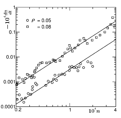
Figure 6: Plots of $dn/dt$ versus $n$, n being the droplet density. Results from two values of $\rho$, in $d=3$, are included. The solid lines are proportional to $n^{2}$. For $\rho=0.08$ a multiplicative factor $5$ was used to separate the data sets from each other. From J. Chem. Phys. 139, 044911 (2013).

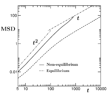
Figure 7: Mean squared displacements for droplets in equilibrium and nonequilibrium situations are plotted versus time. The droplets are of similar size. The quadratic and linear behavior, corresponding to ballistic and diffusive regimes, are appropriately marked by different lines. The results corresponds to $d=3$. From Soft Matter 9, 4178 (2013).

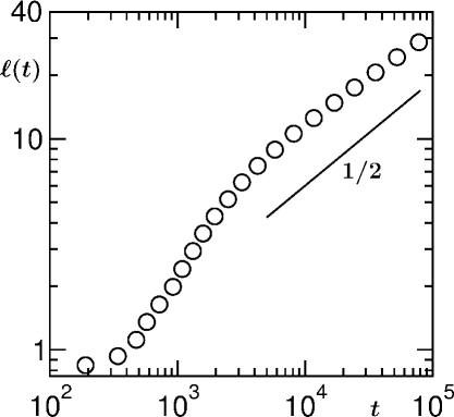
Figure 8: Plot of $\ell$ vs $t$, obtained from the simulations of LJ fluid in $d=2$. The solid line has $t^{1/2}$ behavior. The results correspond to droplet morphology for overall density $\rho=0.02$.

In Fig.6 we show plots of $dn/dt$ versus $n$, for two different low values of $\rho$, both providing droplet structure, on a double-log scale. Technical details on the counting of droplets by identifying them can be found elsewhere SRoy1 ; SRoy2 ; SRoy3 . Linear look in both the cases confirm power-law behavior. The solid lines there are proportional to $n^{2}$ with which the simulation data are consistent. This verifies the starting equation [see Eq.(12)] for deriving the BS KBinder3 ; KBinder4 ; EDSiggia growth law. Thus, the possibility of a LS IMLifshitz mechanism is ruled out. We have also checked that between two collisions, sizes of droplets remain same, within minor fluctuations. This further discards the importance of LS mechanism in the present context.

Next, we come to the point of inter-droplet interaction. To understand it we have calculated the MSD JPHansen of individual droplets SRoy1 ; SRoy2 as

$${\rm{MSD}}=<(\vec{R}_{CM}(t)-\vec{R}_{CM}(0))^{2}>,$$ (27)

where $\vec{R}_{\rm{CM}}(t)$ is the location of the centre of mass of the droplet under consideration at time $t$. In Fig. 7 we show MSD for a typical droplet during nonequilibrium evolution, as a function of time. Note that the duration over which such data can be presented is dictated by the average collision interval. This is larger for low droplet density and increases with the evolution of the system. In the same graph we showed a corresponding plot for a droplet in equilibrium situation, of approximately the same size as the nonequilibrium case. The difference between the two cases is significant. On a double-log scale, at late time, the equilibrium droplet exhibits linear behavior, confirming Brownian motion. The super-linear behavior in the nonequilibrium case is due to inter-droplet interaction, as stated by Tanaka HTanaka1 ; HTanaka2 ; HTanaka3 .

Finally, in Fig.8 we show $\ell$ versus $t$ plot in $d=2$ for off-critical composition JMidya . Here clearly an exponent $\alpha=1/2$ is visible. From the calculation of $dn/dt$, in this dimension also we have confirmed that the mechanism is BS. For the sake of brevity we do not present these here. For higher overall density, the interface diffusion mechanism in this dimension was previously observed SWKoch .

V Conclusion

We have provided a brief review on kinetics of fluid phase separation. A general discussion on various theoretical pictures, based on the system dimensionality and domain morphology, is provided. Methodologies related to coarse-grained and atomistic models are discussed. Particular emphasis was on the molecular dynamics simulation methods.

Molecular dynamics results for vapor-liquid transitions are presented SKDas2 ; HKabrede ; SMajumder3 ; SRoy1 ; SRoy2 ; SRoy3 ; JMidya in $d=2$ and $3$. These include percolating as well as droplet structures. The domain growths from these simulations are observed to be consistent with theoretical predictions, despite the fact that most of these predictions are related to phase separation in binary fluids. For brevity, we have avoided results on binary fluid mixtures.

Recently, important results have been obtained with respect to aging in fluid phase separation, for binary fluids as well as vapor-liquid systems, via molecular dynamics simulations SAhmad4 ; SMajumder4 . These results are understood via simple scaling arguments. In addition, effects of disorder in kinetics of fluid phase separation have been looked at SAhmad3 and compared with disordered Ising systems. Lack of space, however, restricts us from including these results.

Further, there have been significant activities in the area of kinetics in confined geometry RALJones2 ; SPuri3 ; HTanaka4 ; SBastea ; SKDas4 ; SKDas5 ; MJAHore ; KBinder5 ; PKJaiswal1 ; PKJaiswal2 ; EAGJamie . In computational front, good number of reports exist in fluid phase separation SKDas4 ; SKDas5 ; MJAHore ; KBinder5 ; PKJaiswal2 ; EAGJamie as well. However, the understanding of these results are not as complete as pure two- and three- dimensional systems.

Even though there exists significant agreement between theories and simulations of simple models, the situation is not as satisfactory as far as experiments are concerned. Discrepancy between theoretical predictions and experimental observations can be attributed to the presence of impurities in real systems as well as to over-simplified pictures in theoretical calculations. On the other hand, it is possible to do simulation study of more realistic models SAhmad3 ; SJMitchell to obtain better agreement with experiments, for both diffusive and hydrodynamic coarsening, particularly when improved computational resources are available.

Acknowledgement: The work was partially funded by Department of Science and Technology, Government of India. ${*}$ das@jncasr.ac.in

References

- (1) M.E. Fisher, Theory of Equilibrium Critical Phenomena, Rep. Prog. Phys. 30 (1967) 615-730.
- (2) H.E. Stanley, Introduction to Phase Transitions and Critical Phenomena, Oxford University Press, 1971.
- (3) R. Evans, The Nature of the Liquid-Vapor Interface and Other Topics in the Statistical Mechanics of Non-Uniform, Classical Fluids, Adv. Phys. 28 (1979) 143-200.
- (4) K. Binder, Theory of First Order Phase Transitions, Rep. Prog. Phys. 50 (1987) 783-859.
- (5) K. Binder, Spinodal Decomposition, in R.W. Cahn, P. Haasen, E.J. Kramer (Eds.), Materials Science and Technology, Vol-5: Phase Transformation of Material, Weinheim, VCH (1991) 405-471.
- (6) D. Kashchiev, Nucleation: Basic Theory with Applications, Oxford, Butterworth-Heinemann, 2000.
- (7) R.A.L. Jones, Soft Condensed Matter, Oxford University Press, 2002.
- (8) A. Onuki, Phase Transition Dynamics, Cambridge University Press, 2002.
- (9) A.J. Bray, Theory of Phase Ordering Kinetics, Adv. Phys, 51 (2002) 481-587.
- (10) S. Puri and V. Wadhawan (Eds.), Kinetics of Phase Transitions, CRC Press, Boca Raton, 2009.
- (11) S.K. Das, Atomistic simulations of liquid-liquid coexistence in confinement: Comparison of thermodynamics and kinetics with bulk, Molecular Simulation (2014).
- (12) I.M. Lifshitz and V.V. Sloyozov, The Kinetics of Precipitation from Supersaturation Solid Solutions, J. Phys. Chem. Solids, 19 (1961) 35-50.
- (13) D.A. Huse, Correlation to Late-Stage Behavior in Spinodal Decomposition: Lifshitz-Slyozov Scaling and Monte Carlo Simulations, Phys. Rev. B 34 (1986) 7845-7850.
- (14) J.F. Marko and G.T. Barkema, Phase Ordering in the Ising Model with Conserved Spin, Phys. Rev. E 52 (1995) 2522-2534.
- (15) D.W. Heermann, L. Yixne, K. Binder, Scaling Solution and Finite-Size Effects in the Lifshitz-Slyozov Theory, Physica A 230 (1996) 132-148.
- (16) J. Vinals and D. Jasnow, Finite-size-scaling analysis of domain growth in the kinetic Ising model with conserved and nonconserved order parameters, Phys. Rev. B 37 (1998) 9582-9589.
- (17) S. Majumder and S.K. Das, Domain Coarsening in Two Dimensions: Conserved Dynamics and Finite-Size Scaling, Phys. Rev. E 81 (2010) 050102.
- (18) S. Majumder and S.K. Das, Temperature and Composition Dependence of Kinetics of Phase Separation in Solid Binary Mixtures, Phys. Chem. Chem. Phys. 15 (2013) 13209.
- (19) T. Blanchard, F. Corberi, L.F. Cugliandolo and M. Pico, How soon after a zero-temperature quench is the fate of the Ising model sealed ?, EPL 106 (2014) 66001.
- (20) K. Binder and D. Stauffer, Theory for the Slowing Down of the Relaxation and Spinodal Decomposition of Binary Mixtures, Phys. Rev. Lett. 33 (1974) 1006-1009.
- (21) K. Binder, Theory for the dynamics of ”clusters.” II. Critical diffusion in binary systems and the kinetics of phase separation, Phys. Rev. B 15 (1977) 4425-4447.
- (22) E.D. Siggia, Late Stages of Spinodal Decomposition in Binary Mixtures, Phys. Rev. A 20 (1979) 595-605.
- (23) H. Furukawa, Effect of Inertia on Droplet Growth in a Fluid, Phys. Rev. A 31 (1985) 1103-1108.
- (24) H. Furukawa, Turbulent Growth of Percolated Droplets in Phase Separating Fluids, Phys. Rev. A 36 (1987) 2288-2292.
- (25) M. San Miguel, M. Grant and J.D. Gunton, Phase Separation in Two-Dimensional Binary Fluids, Phys. Rev. A 31 (1985) 1001-1005.
- (26) H. Tanaka, A new coarsening mechanism of droplet spinodal decomposition, J. Chem. Phys. 103 (1995) 2361.
- (27) H. Tanaka, Coarsening mechanisms of droplet spinodal decomposition in binary fluid mixtures, J. Chem. Phys. 105 (1996) 10099-10114.
- (28) H. Tanaka, New Mechanisms of Droplet Coarsening in Phase-Separating Fluid Mixtures, J. Chem. Phys. 107 (1997) 3734-3737.
- (29) F. Perrot, P. Guenoun, T. Baumberger, D. Beysens, Y. Garrabos, and B. Le Neindre, Nucleation and Growth of Tightly Packed Droplets in Fluids, Phys. Rev. Lett. 73 (1994) 688-691.
- (30) J. P. Delville, C. Lalaude, S. Buil, and A. Ducasse, Late stage kinetics of a phase separation induced by a cw laser wave in binary liquid mixtures, Phys. Rev. E 59 (2006) 5804-5818.
- (31) J. Hobley, S. Kajimoto, A. Takamizawa, and H. Fukumura, Experimentally determined growth exponents during the late stage of spinodal demixing in binary liquid mixtures, Phys. Rev. E 73 (2006) 011502.
- (32) D. Beysens, Y. Garrabos, D. Chatain and P. Evesque, Phase transition under forced vibrations in critical , EPL 86 (2009) 16003.
- (33) S. Tanaka, Y. Kubo, Y. Yokoyama, A. Toda, K. Taguchi and H. Kajioka, Kinetics of phase separation and coarsening in dilute surfactant pentaethylene glycol monododecyl ether solutions , J. Chem. Phys. 135 (2011) 234503.
- (34) V.M. Kendon, M.E. Cates, I. Pagonabarraga, J.C. Desplat and P. Blandon Inertial Effects in Three-Dimensional Spinodal Decomposition of a Symmetric Binary Fluid Mixture: A Lattice Boltzmann Study, J. Fluid. Mech. 440 (2001) 147-203.
- (35) S. Puri and B. Dünweg, Temporally linear domain growth in the segregation of binary fluids, Phys. Rev. A 45 (1992) R6977-R6980.
- (36) C. Datt, S.P. Thampi, and R. Govindarajan, Morphological evolution of domains in spinodal decomposition, Phys. Rev. E 91 (2015) 010101(R).
- (37) M. Laradji, S. Toxvaerd and O.G. Mountain, Molecular dynamics simulation of spinodal decomposition in three-dimensional binary fluids, Phys. Rev. Lett. 77 (1996) 2253-2256.
- (38) A.K. Thakre, W.K. den OHe and W.J. Briels, Domain Formation and Growth in Spinodal Decomposition in a Binary Fluid By Molecular Dynamics Simulations, Phys. Rev. E 77 (2008) 011503.
- (39) S. Ahmad, S.K. Das and S. Puri, Kinetics of Phase Separation In Fluids: A Molecular Dynamics Study, Phys. Rev. E 82 (2010) 040107.
- (40) S. Ahmad, S.K. Das and S. Puri, Crossover in Growth Laws for Phase Separating Binary Fluids: Molecular Dynamics Simulations, Phys. Rev. E 85 (2012) 031140.
- (41) S. Ahmad, S. Puri and S.K. Das, Phase separation of fluids in porous media: A molecular dynamics study, Phys. Rev. E 90 (2014) 040302(R).
- (42) S.K. Das, S. Roy, S. Majumder and S. Ahmad, Finite-size effects in dynamics: Critical versus coarsening phenomena, Phys. Rev. E 97 (2012) 66006.
- (43) H. Kabrede and R. Hentschke, Spinodal Decomposition in a 3D Lennard-Jones System, Physica A 361 (2006) 485-493.
- (44) S. Majumder and S.K. Das, Universality in Fluid Domain Coarsening: The Case of Vapor-Liquid Transition, EPL 95 (2012) 46002.
- (45) S. Roy and S.K. Das, Nucleation and growth of droplets in vapor-liquid transitions, Phys. Rev. E 85 (2012) 050602.
- (46) S. Roy and S.K. Das, Dynamics and growth of dropltes close to the coexistence curve in fluids, Soft Matter 9 (2013) 4178-4187.
- (47) S. Roy and S.K. Das, Effects of domain morphology on kinetics of fluid phase separation, J. Chem. Phys. 139 (2013) 044911.
- (48) S.W. Koch, R.C. Desai and F.F. Abraham, Dynamics of phase separation in two-dimensional fluids: Spinodal decomposition, Phys. Rev. A 27 (1983) 2152-2167.
- (49) J. Midya and S.K. Das, to be published.
- (50) D.S. Fisher and D.A. Huse, Nonequilibrium dynamics of spin glass, Phys. Rev. B 38 (1988) 373-385.
- (51) S.N. Majumdar, A.J. Bray, S.J. Cornell and C.Sire, Global persistence exponent for nonequilibrium critical dynamics, Phys. Rev. Lett. 77 (1996) 3704-3707.
- (52) J.-P. Hansen and I.R. McDonald, Theory of Simple Liquids, Academic Press, London, 2008.
- (53) D.P. Landau and K. Binder, A Guide to Monte Carlo simulations in statistical physics, Cambridge University Press.
- (54) I. Schmidt and K. Binder, Dynamics of wetting transitions: A time-dependent Ginzburg-Landau treatment, Z. Phys. B: Condens. Matter 67 (1987) 369.
- (55) S.K. Das, J. Horbach and K. Binder, Kinetics of phase separation in thin films: Lattice versus continuum models for solid binary mixtures, Phys. Rev. E 79 (2009) 021602.
- (56) M.P. Allen and D.J. Tildesley, Computer Simulations of Liquid, Oxford, Clarendon, 1987.
- (57) K. Kaski, K. Binder and J.D. Gunton, A study of cell distribution functions of the three dimensional Ising model, Phys. Rev. B 29 (1984) 3996-4009.
- (58) S. Ramaswamy, The mechanics and statistics of active matter, Annu. Rev. Condens. Matter Phys. 1 (2010) 323-345.
- (59) D. Frenkel and B. Smit, Understanding Molecular Simulation: From alforithms to applications, San Diego, Academic Press, 2002.
- (60) D.C. Rapaport, The Art of Molecular DYnamics Simulations, Cambridge University Press, 2004.
- (61) P. Nikuman, M. Karttunen and I. Vattulainen, How would you integrate the equations of motion in dissipative particle dynamics simulations ?, Comp. Phys. Comm. 153 (2003) 407-423.
- (62) S.D. Stoyanov and R.D. Groot, From molecular dynamics to hydrodynamics: A novel Galilean invariant thermostat, J. Chem. Phys. 122 (2005) 114112.
- (63) C. Pastorino, T. Kreer, M. Müller and K. Binder, Comparison of dissipative particle dynamics and Langevin thermostats for out-of-equilibrium simulations of polymsic systems, Phys. Rev. E 76 (2007) 026706.
- (64) A. Winkler, P. Virnau, K. Binder, R.G. Winkler and G. Gompper, Hydrodynamic mechanisms of spinodal decomposition in confined colloid-polymer mixtures: A multiparticle collision dynamics study, J. Chem. Phys. 138 (2013) 0544901.
- (65) E.A. Koopman and C.P. Lowe, Advantages of a Lowe-Andersen thermostat in molecular dynamics simulations, J. Chem. Phys. 124 (2006) 204103.
- (66) S. Roy and S.K. Das, Finite-size scaling study of shear viscosity anomaly at liquid-liquid criticality, J. Chem. Phys. 141 (2014) 234502.
- (67) M.E. Fisher and M.N. Barber, Scaling theory for finite-size effects in the critical region, Phys. Rev. Lett. 28 (1972) 1516-1519.
- (68) S. Ahmad, F. Corberi, S.K. Das, E. Lippiello, S. Puri and M. Zannetti, Aging and crossover in phase separating fluid mixtures, Phys. Rev. E 86 (2012) 061129.
- (69) S. Majumder and S.K. Das, Effects of density conservation and hydrodynamics on aging in nonequlibrium processes, Phys. Rev. Lett. 111 (2013) 055503.
- (70) R.A. L. Jones, Laura J. Norton, Edward J. Kramer, Frank S. Bates, and Pierre Wiltzius, Surface-directed spinodal decomposition Phys. Rev. Lett. 66 (1991) 1326-1329.
- (71) S. Puri and K. Binder, Surface-directed spinodal decomposition: Phenomenology and numerical results, Phys. Rev. A 46 (1992) R4487-R4489.
- (72) H. Tanaka, Interplay between wetting and phase separation in binary fluid mixtures: roles of hydrodynamics, J. Phys.: Condens. Matter 13 (2001) 4637-4674.
- (73) S. Bastea, S. Puri, and J.L. Lebowitz, Surface-directed spinodal decomposition in binary fluid mixtures, Phys. Rev. E 63 (2001) 041513.
- (74) S.K. Das, S. Puri, J. Horbach, and K. Binder, Spinodal decomposition in thin films: Molecular-dynamics simulations of a binary Lennard-Jones fluid mixture, Phys. Rev. E 73 (2001) 031604.
- (75) S.K. Das, S. Puri, J. Horbach, and K. Binder, Molecular Dynamics Study of Phase Separation Kinetics in Thin Films, Phys. Rev. Lett. 96 (2006) 016107.
- (76) M.J.A. Hore and M. Laradji, Dissipative particle dynamics simulation of the interplay between spinodal decomposition and wetting in thin film binary fluids , J. Chem. Phys. 132 (2010) 024908.
- (77) K. Binder, S. Puri, S.K. Das and J. Horback, Phase separation in confined geometries, J. Stat. Phys. 138 (2010) 51-84.
- (78) P.K. Jaiswal, K. Binder, and S. Puri, Phase separation of binary mixtures in thin films: Effects of an initial concentration gradient across the film, Phys. Rev. E 85 (2012) 041602.
- (79) P.K. Jaiswal, S. Puri and S.K. Das, Hydrodynamic crossovers in surface-directed spinodal decomposition and surface enrichment , EPL 97 (2012) 16005.
- (80) E.A.G. Jamie, R.P.A. Dullens and D.G.A.L. Aarts, Spinodal decomposition of a confined colloid-polymer system, J. Chem. Phys. 137 (2012) 204902.
- (81) S.J. Mitchell and D.P. Landau, Phase Separation in a Compressible Ising model, Phys. Rev. Lett. 97 (2006) 025701.