Cross-diffusion induced Turing instability in two-prey one-predator system

Abstract

In this paper, we study a strongly coupled two-prey one-predator system. We first prove the unique positive equilibrium solution is globally asymptotically stable for the corresponding kinetic system (the system without diffusion) and remains locally linearly stable for the reaction-diffusion system without cross-diffusion, hence it does not belong to the classical Turing instability scheme. Moreover we prove that the positive equilibrium solution is globally asymptotically stable for the reaction-diffusion system without cross-diffusion. But it becomes linear unstable only when cross-diffusion also plays a role in the reaction-diffusion system, thus it is a cross-diffusion induced instability. Finally, the corresponding numerical simulations are also demonstrated and we obtain the spatial patterns.

1 Introduction

In 2009, Elettreby considered the following prey-predator model [3]

$$\left\{\begin{array}[]{l}\displaystyle u_{1}^{\prime}=au_{1}(1-u_{1})-u_{1}u_{3}:=u_{1}f_{1}(u_{1},u_{3}),\\ \displaystyle u_{2}^{\prime}=bu_{2}(1-u_{2})-u_{2}u_{3}:=u_{2}f_{2}(u_{2},u_{3}),\\ \displaystyle u_{3}^{\prime}=-cu_{3}^{2}+(du_{1}+eu_{2})u_{3}:=u_{3}f_{3}(u_{1},u_{2},u_{3}),\end{array}\right.$$ (1.4)

where $u_{1},u_{2}$ and $u_{3}$ are the population densities of three species. This system models the dynamic of two-prey one-predator ecosystem, i.e. the third species preys on the second and the first one. In the absence of any predation, each term of preys grows logistically. The effect of the predation is to reduce the prey growth rate. In the absence of any prey for sustenance, the predator’s death rate results in inverse decay, which is the term $-cu_{3}^{2}$. The prey’s contribution to growth rate of the predators are respectively $du_{1}u_{3}$ and $eu_{2}u_{3}$. They studyed the global stability and persistence of the model.

However, in reality, individual organisms are distributed in space. We can use the reaction-diffusion equations to establish spatio-temporal dynamical system which can model the pursuit-evasion phenomenon (predators pursuing prey and prey escaping predators) in the prey-predator system. Therefore, in present paper we further investigate the following reaction-diffusion model with cross-diffusion:

$$\left\{\begin{array}[]{lll}u_{1t}-\Delta[(k_{11}+k_{13}u_{3})u_{1}]=au_{1}(1-u_{1})-u_{1}u_{3},&\mbox{in}\ \Omega\times(0,\infty),\\ u_{2t}-\Delta[(k_{22}+k_{23}u_{3})u_{2}]=bu_{2}(1-u_{2})-u_{2}u_{3},&\mbox{in}\ \Omega\times(0,\infty),\\ u_{3t}-\Delta[(k_{31}u_{1}+k_{32}u_{2}+k_{33})u_{3}]=-cu_{3}^{2}+(du_{1}+eu_{2})u_{3},&\mbox{in}\ \Omega\times(0,\infty),\\ \frac{\partial u_{1}}{\partial\eta}=\frac{\partial u_{2}}{\partial\eta}=\frac{\partial u_{3}}{\partial\eta}=0,&\mbox{on}\ \partial\Omega\times(0,\infty),\\ u_{1}(x,0)=u_{10}(x),u_{2}(x,0)=u_{20}(x),u_{3}(x,0)=u_{30}(x),&\mbox{in}\ \ \Omega,\end{array}\right.$$ (1.10)

where $\Omega$ is a bounded domain in $R^{N}$ with smooth boundary $\partial\Omega$. $\eta$ is the unit outward normal to $\partial\Omega$. The homogeneous Neumann boundary condition indicates that there is zero population flux across the boundary. The parameters $a,b,c,d,e$ and $k_{ij}$ $(1\leq i$, $j\leq 3)$ are all positive constants. $k_{ii}$ is the diffusion rate of $i$-th species. This diffusion term represent simple Brownian type motion of particle dispersal. $k_{ij}$ $(i\neq j)$ is the cross-diffusion rate of $i$-th species. It is necessary to note that the cross-diffusion coefficient may be positive or negative. The positive cross-diffusion coefficient represents that one species tends to move in the direction of lower concentration of another species. On the contrary, the negative cross-diffusion coefficient denotes the population flux of one species in the direction of higher concentration of another species. Here the cross-diffusion term presents the tendency of predators to avoid the group defense by a large number of prey, i.e. the predator diffuses in the direction of lower concentration of the prey species. More biological background can be found in [1, 14, 17].

As we know, the problem of cross-diffusion was proposed first by Kerner [9] and first applied to competitive population systems by Shigesada et al. [20]. Since then, the role of cross-diffusion in the models of many physical, chemical and biological processes has been extensively studied. In the field of population dynamics some models of multispecies population are described by reaction-diffusion systems. Jorne [8] examined the effect of cross diffusion on the diffusive Lotka-Volterra system. They found that the cross-diffusion may give rise to instability in the system, although this situation seems quite rare from an ecological point of view. Gurtin [6] developed some mathematical models for population dynamics with the inclusion of cross-diffusion as well as self-diffusion and showed that the effect of cross-diffusion may give rise to the segregation of two species. Some conditions for the existence of global solutions have been given by several authors, for example, Deuring [2], Kim [10], Pozio and Tesei [19], Yamada [25]. Moreover, due to a most interesting qualitative feature: pattern formation induced by cross-diffusion effect there are some works on the diffusion driven instability (Turing instability [22]) and the existence of a non-constant stationary solution, please refer to [11, 12, 13, 15, 16, 18, 23] and the references cited therein.

The main purpose of this paper is to study the Turing instability which is driven solely from the effect of cross-diffusion by using mathematical analysis and numerical simulations. The rest of this paper is organized as follows. In section 2 we show that the unique positive equilibrium of the ODE system (1.4) is globally asymptotically stable. In the section 3 we show that the positive equilibrium remains linearly stable in the presence of self-diffusion. It becomes linearly unstable with the inclusion of some appropriate cross-diffusion influences. The Turing instability occurs only when the cross-diffusion rates $k_{23}$ and $k_{32}$ are large. The resulting patterns are computed by a numerical method and also we devoted to some conclusions in section 4.

2 Stability of the positive equilibrium solution of the ODE system

In this section, we consider the stability of the positive equilibrium solution of the system (1.4). It is easy to know that if

$$abc>\max\{e(b-a),d(a-b)\}$$ (2.11)

the ODE system (1.4) has a unique positive equilibrium $\mathbf{\bar{u}}=(\bar{u}_{1},\bar{u}_{2},\bar{u}_{3})$ which is given by

$$\bar{u}_{1}=\frac{abc+ae-be}{abc+bd+ae},\ \bar{u}_{2}=\frac{abc+bd-ad}{abc+bd+ae},\ \bar{u}_{3}=\frac{ab(d+e)}{abc+bd+ae}.$$ (2.12)

We have the following result:

Theorem 2.1

The unique positive equilibrium $\mathbf{\bar{u}}$ is globally asymptotically stable for the ODE system $(\ref{eq0})$.

Proof. In order to prove the theorem, we need construct a Lyapunov function for the system (1.4).

$$V(\mathbf{u}(t))=d(u_{1}-\bar{u}_{1}-\bar{u}_{1}\ln\frac{u_{1}}{\bar{u}_{1}})+e(u_{2}-\bar{u}_{2}-\bar{u}_{2}\ln\frac{u_{2}}{\bar{u}_{2}})+(u_{3}-\bar{u}_{3}-\bar{u}_{3}\ln\frac{u_{3}}{\bar{u}_{3}}).$$ (2.13)

Then $V(\mathbf{\bar{u}})=0$ and $V(\mathbf{u})>0$ if $\mathbf{u}\neq\mathbf{\bar{u}}$. By using (1.4), we compute

$$\frac{\mathrm{d}V}{\mathrm{d}t} = d(1-\frac{\bar{u}_{1}}{u_{1}})u_{1}^{\prime}+e(1-\frac{\bar{u}_{2}}{u_{2}})u_{2}^{\prime}+(1-\frac{\bar{u}_{3}}{u_{3}})u_{3}^{\prime}$$

$$= d(u_{1}-\bar{u}_{1})[-a(u_{1}-\bar{u}_{1})-(u_{3}-\bar{u}_{3})]+e(u_{2}-\bar{u}_{2})[-b(u_{2}-\bar{u}_{2})-(u_{3}-\bar{u}_{3})]$$

$$+(u_{3}-\bar{u}_{3})[-c(u_{3}-\bar{u}_{3})+d(u_{1}-\bar{u}_{1})+e(u_{2}-\bar{u}_{2})]$$

$$= -ad(u_{1}-\bar{u}_{1})^{2}-be(u_{2}-\bar{u}_{2})^{2}-c(u_{3}-\bar{u}_{3})^{2}<0$$

for all $\mathbf{u}\neq\mathbf{\bar{u}}$. By the Lyapunov-LaSalle invariance principle [7], $\bar{\mathbf{u}}$ given by (2.12) is globally asymptotically stable for the kinetic system (1.4).

Theorem 2.2

The unique positive equilibrium $\mathbf{\bar{u}}$ is globally asymptotically stable for the reaction-diffusion system $(\ref{eq1})$ without cross-diffusion, i.e. $k_{ij}=0$ for $i\neq j$.

Proof. To study the global behavior of system (1.2), we introduce the following Lyapunov functional

$$W(t)=\int_{\Omega}V(\mathbf{u}(x,t))\mathrm{d}x$$ (2.14)

where $V(\mathbf{u}(x,t))$ is given by (2.13). By direct computation, we have

$$\frac{\mathrm{d}W}{\mathrm{d}t} = \int_{\Omega}\mbox{grad}_{\mathbf{u}}V\cdot\frac{\partial\mathbf{u}}{\partial t}\mathrm{d}x$$

$$= \int_{\Omega}\left(d(1-\frac{\bar{u}_{1}}{u_{1}}),e(1-\frac{\bar{u}_{2}}{u_{2}}),(1-\frac{\bar{u}_{3}}{u_{3}})\right)\cdot(k_{11}\Delta u_{1}+u_{1}f_{1},k_{22}\Delta u_{2}+u_{2}f_{2},$$

$$k_{33}\Delta u_{3}+u_{3}f_{3})\mathrm{d}x$$

$$= \int_{\Omega}d\left(k_{11}(1-\frac{\bar{u}_{1}}{u_{1}})\Delta u_{1}\right)\mathrm{d}x+\int_{\Omega}e\left(k_{22}(1-\frac{\bar{u}_{2}}{u_{2}})\Delta u_{2}\right)\mathrm{d}x$$

$$+\int_{\Omega}\left(k_{33}(1-\frac{\bar{u}_{3}}{u_{3}})\Delta u_{3}\right)\mathrm{d}x+\int_{\Omega}\frac{\mathrm{d}V}{\mathrm{d}t}\mathrm{d}x.$$

From Green’s identity, it follows that

$$\int_{\Omega}\left(k_{ii}(1-\frac{\bar{u}_{i}}{u_{i}})\Delta u_{i}\right)\mathrm{d}x = \int_{\partial\Omega}k_{ii}(1-\frac{\bar{u}_{i}}{u_{i}})\frac{\partial u_{i}}{\partial n}\mathrm{d}S-\int_{\Omega}k_{ii}\nabla_{x}(1-\frac{u_{i}}{u_{i}})\cdot\nabla_{x}u_{i}\mathrm{d}x$$

$$= -\int_{\Omega}k_{ii}\bar{u}_{i}u_{i}^{-2}|\nabla_{x}u_{i}|^{2}\mathrm{d}x\leq 0.$$

Since $\frac{\mathrm{d}V}{\mathrm{d}t}\leq 0$, $\int_{\Omega}\frac{\mathrm{d}V}{\mathrm{d}t}\leq 0$. Thus, $\frac{\mathrm{d}W}{\mathrm{d}t}<0$  for all $\mathbf{u}\neq\bar{\mathbf{u}}$. By the Lyapunov-LaSalle invariance principle[7], $\bar{\mathbf{u}}$ is globally asymptotically stable for the reaction-diffusion system (1.10) without cross-diffusion.

3 Effects of cross-diffusion on Turing instability

For simplicity, we denote

$$\mathbf{K}(\mathbf{u})=\left(\begin{array}[]{c}(k_{11}+k_{13}u_{3})u_{1}\\ (k_{22}+k_{23}u_{3})u_{2}\\ (k_{31}u_{1}+k_{32}u_{2}+k_{33})u_{3}\end{array}\right),\ \ \mathbf{F}(\mathbf{u})=\left(\begin{array}[]{c}au_{1}(1-u_{1})-u_{1}u_{3}\\ bu_{2}(1-u_{2})-u_{2}u_{3}\\ -cu_{3}^{2}+(du_{1}+eu_{2})u_{3}\end{array}\right).$$

Then the reaction-diffusion system (1.10) can be rewritten in matrix notation as:

$$\left\{\begin{array}[]{lll}\displaystyle\frac{\partial\mathbf{u}}{\partial t}-\Delta\mathbf{K}(\mathbf{u})=\mathbf{F}(\mathbf{u})&\mbox{in}\ \Omega\times(0,\infty),\\[5.69054pt] \displaystyle\frac{\partial\mathbf{u}}{\partial\eta}=0&\mbox{on}\ \Omega\times(0,\infty),\\[5.69054pt] \mathbf{u}(x,0)=(u_{10}(x),u_{20}(x),u_{30}(x))^{T}&\mbox{in}\ \Omega.\end{array}\right.$$ (3.4)

Linearizing the reaction-diffusion system (3.4) about the positive equilibrium $\bar{\mathbf{u}}=(\bar{u}_{1},\bar{u}_{2},\bar{u}_{3})$, we have

$$\frac{\partial\Psi}{\partial t}-\mathbf{K}_{\mathbf{u}}(\mathbf{\bar{u}})\Delta\Psi=\mathbf{G}_{\mathbf{u}}(\mathbf{\bar{u}})\Psi$$ (3.5)

where $\Psi=(\psi_{1},\psi_{2},\psi_{3})^{T}$ and

$$\mathbf{K}_{\mathbf{u}}(\mathbf{u})=\left(\begin{array}[]{ccc}k_{11}+k_{13}\bar{u}_{3}&0&k_{13}\bar{u}_{1}\\ 0&k_{22}+k_{23}\bar{u}_{3}&k_{23}\bar{u}_{2}\\ k_{31}\bar{u}_{3}&k_{32}\bar{u}_{3}&k_{33}+k_{31}\bar{u}_{1}+k_{32}\bar{u}_{2}\end{array}\right),$$

$$\mathbf{G}_{\mathbf{u}}(\mathbf{u})=\left(\begin{array}[]{ccc}-a\bar{u}_{1}&0&-\bar{u}_{1}\\ 0&-b\bar{u}_{2}&-\bar{u}_{2}\\ d\bar{u}_{3}&e\bar{u}_{3}&-c\bar{u}_{3}\end{array}\right).$$

Let $0=\mu_{1}<\mu_{2}<\mu_{3}<\cdot\cdot\cdot$ be the eigenvalues of the operator $-\Delta$ on $\Omega$ with the homogeneous Neumann boundary condition, and $E(\mu_{i})$ be the eigenspace corresponding to $\mu_{i}$ in $C^{2}(\Omega)$. Let $\mathbf{X}=\{\mathbf{u}\in[C^{1}(\bar{\Omega})]^{3}|\ \frac{\partial\mathbf{u}}{\partial\eta}=0\ \mbox{on}\ \partial\Omega\}$, $\{\phi_{ij}\}_{j=1,2,...,\dim E(\mu_{i})}$ be an orthonormal basis of $E(\mu_{i})$, and $\mathbf{X}_{ij}=\{\mathbf{c}\phi_{ij}|\ \mathbf{c}\in\mathbf{R}^{3}\}$. Then

$$\mathbf{X}=\bigoplus^{\infty}_{i=1}\mathbf{X}_{i}\ \ \mbox{and}\ \ \mathbf{X}_{i}=\bigoplus^{\dim E(\mu_{i})}_{j=1}\mathbf{X}_{ij}.$$

For each $i\geq 1$, $\mathbf{X}_{i}$ is invariant under the operator $\mathbf{K}_{\mathbf{u}}(\mathbf{\bar{u}})\Delta+\mathbf{G}_{\mathbf{u}}(\mathbf{\bar{u}})$. Then problem (3.5) has a non-trivial solution of the form $\Psi=\mathbf{c}\phi\exp(\lambda t)$ if and only if $(\lambda,\mathbf{c})$ is an eigenpair for the matrix $-\mu_{i}\mathbf{K}_{\mathbf{u}}(\mathbf{\bar{u}})+\mathbf{G}_{\mathbf{u}}(\mathbf{\bar{u}})$, where $\mathbf{c}$ is a constant vector. Then the equilibrium $\mathbf{\bar{u}}$ is unstable if at least one eigenvalue $\lambda$ has a positive real part for some $\mu_{i}$.

The characteristic polynomial of $-\mu_{i}\mathbf{K}_{\mathbf{u}}(\mathbf{\bar{u}})+\mathbf{G}_{\mathbf{u}}(\mathbf{\bar{u}})$ is given by

$$\rho_{i}(\lambda)=\lambda^{3}+A_{2i}\lambda^{2}+A_{1i}\lambda+A_{0i},$$ (3.6)

where

$$A_{2i}=(k_{11}+k_{22}+k_{33}+k_{13}\bar{u}_{3}+k_{23}\bar{u}_{3}+k_{31}\bar{u}_{1}+k_{32}\bar{u}_{2})u_{i}+a\bar{u}_{1}+b\bar{u}_{2}+c\bar{u}_{3}$$ (3.7)

$$A_{1i} = [(k_{11}+k_{13}\bar{u}_{3})(k_{22}+k_{23}\bar{u}_{3}+k_{33}+k_{13}\bar{u}_{1}+k_{32}\bar{u}_{2})+(k_{22}+k_{23}\bar{u}_{3})$$ (3.8)

$$(k_{33}+k_{31}\bar{u}_{1}+k_{32}\bar{u}_{2})-k_{23}k_{32}\bar{u}_{2}\bar{u}_{3}-k_{13}k_{31}\bar{u}_{1}\bar{u}_{3}]\mu_{i}^{2}$$

$$+[(b\bar{u}_{2}+c\bar{u}_{3})(k_{11}+k_{13}\bar{u}_{3})+a\bar{u}_{1}(k_{22}+k_{33}+k_{23}\bar{u}_{3}+k_{31}\bar{u}_{1}+k_{32}\bar{u}_{2})\$$

$$+b\bar{u}_{2}(k_{33}+k_{31}\bar{u}_{1}+k_{32}\bar{u}_{2})+c\bar{u}_{3}(k_{22}+k_{23}\bar{u}_{3})+\bar{u}_{2}\bar{u}_{3}(k_{23}e-k_{32})$$

$$+\bar{u}_{1}\bar{u}_{3}(k_{13}d-k_{31})]\mu_{i}+a\bar{u}_{1}(b\bar{u}_{2}+c\bar{u}_{3})+bc\bar{u}_{2}\bar{u}_{3}+e\bar{u}_{2}\bar{u}_{3}+d\bar{u}_{1}\bar{u}_{3}$$

$$A_{0i} = [(k_{33}k_{11}+k_{33}k_{13}\bar{u}_{3}+k_{31}k_{11}\bar{u}_{1}+k_{31}\bar{u}_{1}\bar{u}_{3}+k_{32}k_{11}\bar{u}_{2}+k_{32}k_{13}\bar{u}_{2}\bar{u}_{3})k_{22}$$ (3.9)

$$+(k_{33}k_{11}+k_{33}k_{13}\bar{u}_{3}+k_{31}k_{11}\bar{u}_{1})k_{23}]u_{i}^{3}+[c\bar{u}_{3}(k_{11}+k_{13}\bar{u}_{3})(k_{22}+k_{23}\bar{u}_{3})$$

$$+(k_{33}+k_{31}+k_{32}\bar{u}_{2})[a\bar{u}_{1}(k_{22}+k_{23}\bar{u}_{3})+b\bar{u}_{2}(k_{11}+k_{13}\bar{u}_{3})]$$

$$+(k_{11}+k_{13}\bar{u}_{3})(ek_{23}\bar{u}_{2}\bar{u}_{3})-ak_{23}k_{32}\bar{u}_{1}\bar{u}_{2}\bar{u}_{3}+dk_{13}\bar{u}_{1}\bar{u}_{3}(k_{22}+k_{23}\bar{u}_{3})$$

$$-k_{13}k_{31}b\bar{u}_{1}\bar{u}_{2}\bar{u}_{3}-k_{31}k_{22}\bar{u}_{1}\bar{u}_{2}-k_{31}k_{32}\bar{u}_{1}\bar{u}_{3}^{2}]\mu_{i}^{2}+[ac\bar{u}_{1}\bar{u}_{3}(k_{22}+k_{23}\bar{u}_{3})$$

$$+bc\bar{u}_{2}\bar{u}_{3}(k_{11}+k_{13}\bar{u}_{3})+ab\bar{u}_{1}\bar{u}_{2}(k_{33}+k_{31}\bar{u}_{1}+k_{32}\bar{u}_{2})+e\bar{u}_{2}\bar{u}_{3}(k_{11}$$

$$+k_{13}\bar{u}_{3})+a\bar{u}_{1}(ek_{23}\bar{u}_{2}\bar{u}_{3}-k_{23}\bar{u}_{2}\bar{u}_{3})+k_{11}\bar{u}_{1}\bar{u}_{2}\bar{u}_{3}bd$$

$$+d\bar{u}_{1}\bar{u}_{3}(k_{22}+k_{23}\bar{u}_{3}-k_{31}b\bar{u}_{1}\bar{u}_{2}\bar{u}_{3})]u_{i}+(abc+ae+bd)\bar{u}_{1}\bar{u}_{2}\bar{u}_{3}.$$

Let $\lambda_{1i},\lambda_{2i},\lambda_{3i}$ be the three roots of (3.6). In order to obtain the stability of $\bar{\mathbf{u}}$, we need to show that three exists a positive constant $\delta$ such that

$$Re\{{\lambda_{1i}}\},Re\{{\lambda_{2i}}\},Re\{{\lambda_{3i}}\}<-\delta,\ \mbox{for all}\ i\geq 1.$$ (3.10)

The aim of the following theorem is to prove that the diffusion alone (with out cross-diffusion, i.e $k_{31}=k_{13}=k_{32}=k_{23}=0$) can not drive instability for this model.

Theorem 3.1

Suppose that $(\ref{H})$ holds and $k_{13}=k_{31}=k_{23}=k_{32}=0$. Then the positive equilibrium $\bar{\mathbf{u}}$ of $(\ref{eq21})$ is linearly stable.

Proof: Substituting $k_{13}$=$k_{31}$=$k_{23}$=$k_{32}=0$ into (3.7), (3.8) and (3.9) we have

$$A_{2i} = a\bar{u}_{1}+b\bar{u}_{2}+c\bar{u}_{3}+(k_{11}+k_{22}+k_{33})\mu_{i}>0$$

$$A_{1i} = (k_{11}k_{22}+k_{11}k_{33}+k_{22}k_{33})\mu_{i}^{2}+[a(k_{22}+k_{33})\bar{u}_{1}+b(k_{11}+k_{33})\bar{u}_{2}+c(k_{11}+k_{22})\bar{u}_{3}]\mu_{i}\qquad\quad$$

$$+ab\bar{u}_{1}\bar{u}_{2}+ac\bar{u}_{1}\bar{u}_{3}+d\bar{u}_{1}\bar{u}_{3}+bc\bar{u}_{2}\bar{u}_{3}+e\bar{u}_{2}\bar{u}_{3}>0$$

$$A_{0i} = k_{11}k_{22}k_{33}\mu_{i}^{3}+(k_{11}k_{22}c\bar{u}_{3}+k_{11}k_{33}b\bar{u}_{2}+k_{22}k_{33}a\bar{u}_{1})\mu_{i}^{2}$$

$$+(abk_{33}\bar{u}_{1}\bar{u}_{2}+dk_{22}\bar{u}_{1}\bar{u}_{2}+ack_{22}\bar{u}_{1}\bar{u}_{3}+bck_{11}\bar{u}_{2}\bar{u}_{3}+ek_{11}\bar{u}_{2}\bar{u}_{3}+bdk_{11}\bar{u}_{1}\bar{u}_{2}\bar{u}_{3})\mu_{i}$$

$$+(ae+bd+abc)\bar{u}_{1}\bar{u}_{2}\bar{u}_{3}>0.$$

A direct calculation shows that $A_{2i}A_{1i}-A_{0i}>0$ for all $i\geq 1$. It follows from Routh-Hurwize criterion that all the three roots $\lambda_{1i},\lambda_{2i},\lambda_{3i}$ of $\rho_{i}(\lambda)=0$ have negative real parts for each $i\geq 1$.

Let $\lambda=\mu_{i}\varepsilon$, then

$$\rho_{i}(\lambda)=\mu_{i}^{3}\xi^{3}+A_{2i}\mu_{i}^{2}\xi^{2}+A_{1i}\mu_{i}\xi+A_{0i}=\tilde{\rho}_{i}(\xi).$$

Since $\mu_{i}\rightarrow\infty$, as $i\rightarrow\infty$, we have

$$\bar{\rho}(\xi)=\lim_{i\rightarrow\infty}\frac{\tilde{\rho}_{i}(\xi)}{\mu_{i}^{3}}=\xi^{3}+(k_{11}+k_{22}+k_{33})\xi^{2}+(k_{11}k_{22}+k_{22}k_{33}+k_{11}k_{33})\xi+k_{11}k_{22}k_{33}.$$

Applying the Routh-Hurwitz criterion it follows that the three roots $\xi_{1},\xi_{2},\xi_{3}$ of $\bar{\rho}(\xi)=0$ all have negative real parts. Thus, there exists a positive constant $\bar{\delta}$ such that $Re\{{\xi_{1}}\},Re\{{\xi_{2}}\}$, $Re\{{\xi_{3}}\}\leq-2\bar{\delta}$. By continuity, we see that there exists $i_{0}\geq 1$, such that $\mu_{i0}>1$ and the three roots $\xi_{i1},\xi_{i2},\xi_{i3}$ of $\tilde{\rho}_{i}(\xi)=0$ satisfy $Re\{\xi_{i1}\},Re\{\xi_{i2}\}$, $Re\{\xi_{i3}\}\leq-\mu_{i}\bar{\delta}\leq-\mu_{i0}\bar{\delta}\leq-\bar{\delta}$ for any $i\geq i_{0}$, Let $-\tilde{\delta}=\max_{1\leq i\leq i_{0}}\{Re\{\lambda_{i1}\},Re\{\lambda_{i2}\},Re\{\lambda_{i3}\}\}$ and $\delta=\min\{{\tilde{\delta},\bar{\delta}}\}$, Then (3.10) holds. Consequently the equilibrium $\bar{\mathbf{u}}$ is linearly stable.

Note that $A_{2i}>0,A_{1i}>0,A_{0i}>0$, and $A_{2i}A_{1i}-A_{0i}>0$ if $k_{31}=k_{32}=0$ since the possible negative terms all involve either $k_{31}$ or $k_{32}$. By the same arguments as in Theorem 3.1, we have

Theorem 3.2

Suppose that $(\ref{H})$ holds and $k_{31}=k_{32}=0$, Then the positive equilibrium $\bar{\mathbf{u}}$ of $(\ref{eq1})$ is linearly stable.

Next we consider the Turing instability i.e. the stability of the positive equilibrium $\bar{u}=(\bar{u}_{1},\bar{u}_{2},\bar{u}_{3})$ changing from stable, for the ODE dynamics (1.4), to unstable for the PDE dynamics (1.10). Here we give sufficient conditions on cross-diffusion which drives the instability. $k_{31}$ and $k_{32}$ are chosen as variation parameters.

Theorem 3.3

$(1)$ Suppose that $a\bar{u}_{1}-\bar{u}_{3}<0$. Consider $k_{31}$as the variation parameter, then there exists a positive constant $\delta_{31}$ such that when $k_{31}>\delta_{31}$, the equilibrium $\bar{\mathbf{u}}$ is linearly unstable for some domain $\Omega$.
$(2)$ Suppose that $b\bar{u}_{2}-\bar{u}_{3}<0$. Consider $k_{32}$ as the variation parameter, then there exists a positive constant $\delta_{32}$ such that when $k_{32}>\delta_{32}$, the equilibrium $\bar{\mathbf{u}}$ is linearly unstable for some domain $\Omega$.

Proof: Denote

$$A(\mu)=-(C_{3}\mu^{3}+C_{2}\mu^{2}+C_{1}\mu+C_{0})$$ (3.11)

where

$$C_{3} = [(k_{33}k_{11}+k_{33}k_{13}\bar{u}_{3}+k_{31}k_{11}\bar{u}_{1}+k_{31}\bar{u}_{1}\bar{u}_{3}+k_{32}k_{11}\bar{u}_{2}+k_{32}k_{13}\bar{u}_{2}\bar{u}_{3})k_{22}$$

$$+(k_{33}k_{11}+k_{33}k_{13}\bar{u}_{3}+k_{31}k_{11}\bar{u}_{1})k_{23}]$$

$$C_{2} = [c\bar{u}_{3}(k_{11}+k_{13}\bar{u}_{3})(k_{22}+k_{23}\bar{u}_{3})+(k_{33}+k_{31}+k_{32}\bar{u}_{2})[a\bar{u}_{1}(k_{22}+k_{23}\bar{u}_{3})$$

$$+b\bar{u}_{2}(k_{11}+k_{13}\bar{u}_{3})]+(k_{11}+k_{13}\bar{u}_{3})(ek_{23}\bar{u}_{2}\bar{u}_{3})-ak_{23}k_{32}\bar{u}_{1}\bar{u}_{2}\bar{u}_{3}$$

$$+dk_{13}\bar{u}_{1}\bar{u}_{3}(k_{22}+k_{23}\bar{u}_{3})-k_{13}k_{31}b\bar{u}_{1}\bar{u}_{2}\bar{u}_{3}-k_{31}k_{22}\bar{u}_{1}\bar{u}_{2}-k_{31}k_{32}\bar{u}_{1}\bar{u}_{3}^{2}]$$

$$C_{1} = [ab\bar{u}_{1}\bar{u}_{2}k_{31}(a\bar{u}_{1}-\bar{u}_{3})+a\bar{u}_{1}\bar{u}_{2}k_{32}(b\bar{u}_{2}-\bar{u}_{3})+ac\bar{u}_{1}\bar{u}_{3}(k_{22}+k_{23}\bar{u}_{3})+$$

$$bc\bar{u}_{2}\bar{u}_{3}(k_{11}+k_{13}\bar{u}_{3})+ab\bar{u}_{1}\bar{u}_{2}k_{33}+e\bar{u}_{2}\bar{u}_{3}(k_{11}+k_{13}\bar{u}_{3})+aek_{23}\bar{u}_{1}\bar{u}_{2}\bar{u}_{3}$$

$$+k_{11}bd\bar{u}_{1}\bar{u}_{2}\bar{u}_{3}+d\bar{u}_{1}\bar{u}_{3}(k_{22}+k_{23}\bar{u}_{3})$$

$$C_{0} = (abc+ae+bd)\bar{u}_{1}\bar{u}_{2}\bar{u}_{3}.$$

Case 1: $k_{31}$ is the variation parameter.
We assume that $a\bar{u}_{1}-\bar{u}_{3}<0$. The following arguments by continuation are based on the fact that each root of the algebraic equation (3.11) is a continuous function of the variation parameter $k_{31}$. It is easy to prove that equation (3.11) has three real roots $\mu_{1}^{(i)}=\mu_{1}^{(i)}(k_{31})$, $i=1,2,3$ when $k_{31}$ goes to infinity and they are $\lim_{k_{31}\rightarrow\infty}\mu_{1}^{(1)}(k_{31})<0$, $\lim_{k_{31}\rightarrow\infty}\mu_{1}^{(2)}(k_{31})=0$ and $\lim_{k_{31}\rightarrow\infty}\mu_{1}^{(3)}(k_{31})>0$. By continuation, there exists a positive constant $\delta_{31}$ such that when $k_{31}>\delta_{31}$, $C_{1}>0$ and $\det(A(\mu))$ has three real roots. Because $C_{3}>0$ and $C_{0}>0$, the mumber of sign changes of (3.11) is exactly two. Therefore by Descartes’rule, the three real roots have the following properties:
(1) $-\infty<\mu_{1}^{(1)}<0<\mu_{1}^{(2)}<\mu_{1}^{(3)}<\infty,$
(2) $\det(A({\mu}))>0$ if $\mu\in(-\infty,\mu_{1}^{(1)})\cup(\mu_{1}^{(2)},\mu_{1}^{(3)}),$
(3) $\det(A({\mu}))<0$ if $\mu\in(\mu_{1}^{(1)},\mu_{1}^{(2)})\cup(\mu_{1}^{(3)},\infty).$

If $\mu_{i}\in(\mu_{1}^{(2)},\mu_{1}^{(3)})$ for some $i$, then det$(A{(\mu_{i})})>0$ by (2), and consequently $A_{0i}=-\det(A_{(i)})<0$. The number of sign of changes of the characteristic polynomial (3.6) $\rho_{i}(\lambda)=\lambda^{3}+A_{2i}\lambda^{2}+A_{1i}\lambda+A_{0i}$ is either one or three. By Descartes’rule, the characteristic polynomial (3.6) has at least one positive eigenvalue. Hence, the equilibrium $\bar{\mathbf{u}}$ of (1.10) is linearly unstable for any domain $\Omega$ on which at least one eigenvalue $\mu_{i}$ of $-\Delta$ is in the interval $(\mu_{1}^{(2)},\mu_{1}^{(3)})$.

Case 2: $k_{32}$ is the variation parameter.
We assume that $b\bar{u}_{2}-\bar{u}_{3}<0$. The following arguments by continuation are based on the fact that each root of the equation (3.11) is a continuous function of the variation $k_{32}$. It is easy to prove that equation (3.11) has three real roots $\mu_{2}^{(i)}=\mu_{2}^{(i)}(k_{32})$, $i=1,2,3$ when $k_{32}$ goes to infinity and they are $\lim_{k_{32}\rightarrow\infty}\mu_{2}^{{(1)}}(k_{32})<0$, $\lim_{k_{32}\rightarrow\infty}\mu_{2}^{(2)}(k_{32})=0$ and $\lim_{k_{32}\rightarrow\infty}\mu_{2}^{(3)}(k_{32})>0$. By continuation, there exists a positive constant $\delta_{32}$ such that when $k_{32}>\delta_{32}$, $C_{1}>0$ and $\det(A(\mu))$ has three real roots. Because $C_{3}>0$ and $C_{0}>0$, the mumber of sign changes of (3.11) is exactly two. Therefore by Descartes’rule,the three real roots have the folloeing properties:
(1) $-\infty<\mu_{2}^{(1)}<0<\mu_{2}^{(2)}<\mu_{2}^{(3)}<\infty$,
(2) $\det(A({\mu}))>0\ \mbox{if}\ \mu\in(-\infty,\mu_{2}^{(2)})\bigcup(\mu_{2}^{(2)},\mu_{2}^{(3)})$,
(3) $\det(A({\mu}))<0\ \mbox{if}\ \mu\in(\mu_{2}^{(1)},\mu_{2}^{(2)})\bigcup(\mu_{2}^{(3)},\infty)$.

If $\mu_{i}\in(\mu_{2}^{(2)},\mu_{2}^{(3)})$ for some $i$, then $\det(A{(\mu_{i})})>0$, and consequently $A_{0i}=-\det(A_{(i)})<0$. By similar argument as case 1, The number of sign of changes of the characteristic polynomial (3.6) $\rho_{i}(\lambda)=\lambda^{3}+A_{2i}\lambda^{2}+A_{1i}\lambda+A_{0i}$ is either one or three. By Descartes’rule, the characteristic polynomial (3.6) has at least one positive eigenvalue. Hence, the equilibrium $\bar{u}$ of (1.10) is linearly unstable for any domain $\Omega$ on which at least one eigenvalue $\mu_{i}$ of $-\Delta$ is in the interval $(\mu_{2}^{(2)},\mu_{2}^{(3)})$.

Remark 3.1

$(i)$ In Theorem 3.3, the condition $a\bar{u}_{1}-\bar{u}_{3}<0$ and $b\bar{u}_{2}-\bar{u}_{3}<0$ are compatible with the condition $(2.3)$ respectively.

$(ii)$ $k_{31}$ and $k_{32}$ can be chosen as variation parameters because the number of sign of change for the polynomial $(3.8)$ could be bigger than one for large values of $k_{31}$ or $k_{32}$, By descartes’ rule, the polynomial $(3.8)$ could have positive roots which lead to linear instability.

$(iii)$ Biological interpretation: In our model, the third species preys on the first and second one. The positive steady state of the model can be broken by the reaction-diffusion among two species on the model. Case one: In this case, the first species are assumed to reproduce exponentially unless subject to intra-species competitions and predation. This exponential growth is represented in the equation by the term $au_{1}$. The level of intra-species competitions among the first species is assumed to be proportional to the population density of first species by the term $au_{1}$. The rate of predation upon the prey is assumed to be proportional to the rate at which the predators and the prey meet by the term $u_{1}u_{3}$, when the effect on first species due to the fact the third species preys on the first one $\bar{u}_{3}$ are larger than the effects on first species due to the intra-species competitions among first species $a\bar{u}_{1}$, the large cross-diffusion of the third species due to the first species $k_{31}$ can break the stability of the positive steady state. In other words, if the predator has a dominate effect on the decreasing of the prey such as predation rate is lager than the rate of intra-species competitions, then the predator with large cross-diffusion can destabilize the constant steady state. Case two: In this case, the third species shall have a dominate effect on the decreasing of the second species. Because $b\bar{u}_{2}-\bar{u}_{3}<0$ implies $b\bar{u}_{2}<\bar{u}_{3}$, predation rate of third species on the second species is large than the rate of intra-species competitions in second species. The similar situation as in case one happens in the case two: the predator with large cross-diffusion can destabilize the constant steady state.

4 Numerical calculations

In this section, using numerical methods, we illustrate that the cross-diffusion induces spatial patterns. The initial data is taken as a uniformly distributed random perturbation around the equilibrium state $(\bar{u}_{1},\bar{u}_{2},\bar{u}_{3})$ in $\Omega$, with a variance lower than the amplitude of the final patterns. More precisely,

$$u_{10}(x)=\bar{u}_{1}+\eta_{1}(x),\quad u_{20}(x)=\bar{u}_{2}+\eta_{2}(x),\quad u_{30}(x)=\bar{u}_{3}+\eta_{3}(x),$$

where $\eta_{i}\in[-1.5,1.5]$ for $i=1,2,3$. In view of Theorems 3.1 and 3.3, the Turing parameter space is (2.11) under which spatial patterns can occur. Thus, in the system (1.10) we fix $a=1$, $b=1$, $c=0.1$, $d=0.1$, $e=0.1$, $k_{11}=0.1$, $k_{13}=0.1$, $k_{22}=0.1$, $k_{23}=0.1$, $k_{31}=0.1$, $k_{33}=0.1$.

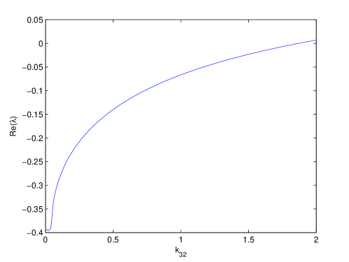
Figure 1: Dispersion relation for the real part of the eigenvalues, $\mathrm{Re}(\lambda)$ versus the cross-diffusion coefficient $k_{32}$.

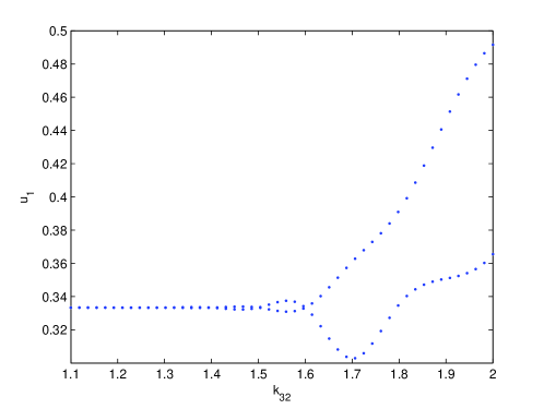
Figure 2: Bifurcation diagram for Turing onset. Maximum and minimum $u_{1}$ for different cross-diffusion in the transition from the homogeneous state to Turing pattern.

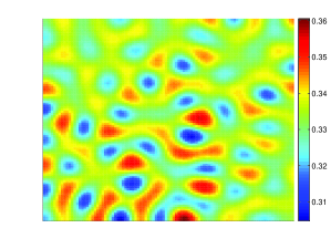
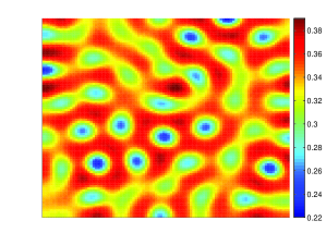
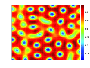
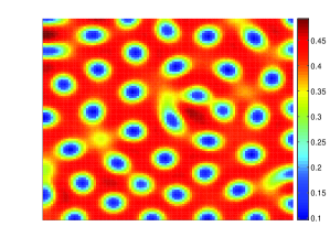
Figure 3: Spatial patterns change quantitatively with different $k_{32}$ as 1.7, 1.8, 1.9, and 2. The other parameters are stated in the text. The steps of the iteration for time is 40000.

In Figure 1, we show that the real part of the eigenvalues $\lambda$ as a function of the cross-diffusion coefficient $d_{32}$. From the characteristic polynomial of (3.6), we can determine the value of $d_{32}$ such that $Re(\lambda)>0$. Now we will implement some numerical simulations for the system (1.10). The domain is confined to a square domain $\Omega=[0,L_{x}]\times[0,L_{y}]\subset\mathbf{R}^{2}$. The wavenumber for this two dimensional domain is thereby

$$\mathbf{k}=\pi(m/L_{x},n/L_{y}),\textrm{ and }|\mathbf{k}|=\pi\sqrt{(m/L_{x})^{2}+(n/L_{y})^{2}},~{}m,n=0,1,\ldots.$$

We consider system (1.10) in a fixed domain $L_{x}=40$ and $L_{y}=40$, and resolve it on a grid with $100\times 100$ sites with the space step of $\triangle x=\triangle y=1$. For the evolution in time, we apply a first order backward Euler time advancing scheme with a time step $\triangle t=0.005$. By discretizing the Laplacian in the grid with lattice sites denoted by $(i,j)$, the nine-point formula is

$$\triangle u|_{(i,j)} =\frac{1}{6\triangle x^{2}}[4a_{l}(i,j)u(i-1,j)+4a_{r}(i,j)u(i+1,j)+4a_{d}(i,j)u(i,j-1)$$

$$+4a_{u}(i,j)u(i,j+1)+a_{l}(i,j)u(i-1,j+1)+a_{u}(i,j)u(i+1,j+1)$$

$$+a_{d}(i,j)u(i-1,j-1)+a_{r}(i,j)u(i+1,j-1)-20u(i,j)],$$

where the matrix elements of $a_{l},a_{r},a_{d},a_{u}$ are unity except at the boundary. When $(i,j)$ is at the left boundary, that is $i=0$, we define $a_{l}(i,j)u(i-1,j)\equiv u(i+1,j)$, which guarantees zero-flux of reactants in the left boundary. Similarly we define $a_{r}(i,j)$, $a_{d}(i,j)$, $a_{u}(i,j)$ such that the boundary is no-flux. The nine-point formula for the Laplacian can have a one-step error of $O(\triangle x^{4})$.

In Figure 2, we compare the density of $u_{1}$ before and after the onset of Turing patterns. Results are qualitatively similar for $u_{2}$ and $u_{3}$, and hence omitted. In the case of $k_{32}$ less than 1.6, i.e. the Turing instability does not occur, we see that the density of $u_{1}$ is homogeneous. In the case of $k_{32}$ larger than 1.6, i.e. Turing instability happen, we see that the density of $u_{1}$ is spatial inhomogeneous.

Now we study the change of the spatial patterns qualitatively and quantitatively with different $k_{32}$. In general, the selection of stripe pattern or spot pattern depends upon the non-linearities of the reaction kinetics. Specifically, it has been shown that the presence of quadratic nonlinearities in the reaction kinetics leads to spot pattern, but the absence of quadratic terms leads to stripe pattern [4]. Noticing that the reaction kinetics of (1.10) only has quadratic nonlinearities, in view of the theory of pattern selection [4], all the spatial patterns are spot patterns. In Figure 3, we also illustrate the quantitative change of the spatial patterns with the different $k_{32}$. From this simulations, we can conclude that with the increasing of $k_{32}$, the spatial patterns converge to regular spotted patterns. The striped patterns can not occur in our model.

5 Comparisons and conclusions

In this paper, we have developed a theoretical framework for studying the phenomenon of pattern formation in a two-prey one-predator system. Applying a stability analysis and suitable numerical simulations, we investigate the Turing parameter space, the associated pattern type and the Turing bifurcation diagram. The proposed approach has applicability to other reaction-diffusion systems including cross-diffusion, such as chemotaxis and cell motility models. In this context, it is of great interest to us the development of a general mathematical and numerical framework that allows for the treatment of certain degenerate quasilinear parabolic systems modeling bacterial growth, that are known to involve several important phenomena such as fractal morphogenesis and branching patterns.

It is worth mentioning that the authors have also the role of cross-diffusion on pattern formation for Lotka-Volterra type models in [5, 21]. In [21], by considering a Holling- Tanner predator-prey model the authors investigated the Turing bifurcation and obtained the pattern selection mechanism. In [5], by studying the Hopf bifurcation the authors attained the spiral patterns. Apart from these work [5, 21], what our model consider is a three species model. The difficulty is that the characteristic equation of our model is a cubic equation. We use the continuity of the cubic functions to overcome it. Our novelty is that we have obtained the bifurcation diagram for Turing onset by numerical simulations, which shows the transition from the homogeneous steady state to the Turing patterns.

It is well-known that for a classical competitive model, the formation of patterns does not occur. We introduce the cross-diffusion into the particular two-prey one-predator model, and show that this gives rise to Turing-like spatial patterns. All this is confirmed with the help of illustrating numerical simulations.

References

[1]R.S. Cantrell, C. Cosner, Spatial Ecology Via Reaction-Diffusion
Equations, Wiley, England, 2003.
[2]P. Deuring, An initial-boundary-value problem for a certain
density-dependent diffusion system, Math. Z. 194(1974) 375-396.
[4]B. Ermentrout, Stripes or spots? Non-linear effects in bifurcation
of reaction-diffusion equations on the square, Proc. R. Soc.
Lond. A 434 (1991) 413-417.
[5]
L.N. Guin, M. Haque and P.K. Mandal, The spatial patterns through diffusion-driven instability in a predator-prey model, Appl. Math. Modell. 36(2012) 1825-1841.
[6]M.E. Gurtin, Some mathematical models for population dynamics that
lead to segregation, Quart. J. Appl. Math. 32(1974) 1-9.
[8]J. Jorne, The diffusive Lotka-Volterra oscillating system, J.
Theoret. Biol. 65(1977) 133-139.
[9]E. H. Kerner, Further considerations on the statistical mechanics of
biological associations, Bull. Math. Biophys. 21(1959) 217-255.
[10]J.U. Kim, Smooth solutions to a quasilinear system of diffusion for
a certain population model, Nonlinear Anal. 21(1984) 657-689.
[11]K. Kuto, Stability of steady-state solutions to a prey-predator
system with cross-diffusion, J. Differ. Equ. 197(2004) 293-314.
[12]K. Kuto, Y. Yamada, Multiple coexistence states for a prey-predator
system with cross-diffusion, J. Differ. Equ. 197(2004) 315-348.
[13]Z. Ling, L. Zhang, Z.G. Lin, Turing pattern formation in a
predator-prey system with cross diffusion, Appl. Math. Modell. 33(2009) 683-691.
[14]Y. Lou, W.M. Ni, Diffusion, self-diffusion and cross-diffusion, J.
Differ. Equ. 131(1996) 79-131.
[15]H. Matano, M. Mimura, Pattern formation in competion-diffusion
systems in nonconvex domains, Publ. RIMS, Kyoto Univ. 19(1983)
1049-1079.
[16]M. Mimura, Stationary pattern of some density-dependent
diffusion system with competitive dynamics, Hiroshima Math. J. 11
(1981) 621-635.
[17]A. Okubo, Diffusion and Ecological Problems: Mathematical Models,
Springer, Berlin, Heidelberg and New York, 1980.
[18]R. Peng, M.X. Wang, G.Y. Yang, Stationary patterns of the
Holling-Tanner prey-predator model with diffusion and
cross-diffusion, Appl. Math. Comput. 196(2008) 570-577.
[19]M. Pozio, A. Tesei, Global existence of a strongly coupled
quasilinear parabolic systems, Nonlinear Anal. 14(1990) 657-689.
[20]N. Shigesada, K. Kawasaki, E. Teramoto, Spatial segregation of
interacting species, J. Theoret. Biol. 79(1979) 83-99.
[21]
G.Q. Sun, Z. Jin, L. Li, M.Haque and B.L. Li, Spatial patterns of a predator-prey model with cross diffusion, Nonlinear Dynamics 69(2012) 1631-1638.
[22]A. Turing, The chemical basis of morphogenesis, Philos. Trans. R.
Soc. B 237(1952) 37-72.
[23]M.X. Wang, Stationary patterns caused by cross-diffusion for a
three-species prey-predator model, Comput. Math. Appl. 52(2006)
707-720.
[24]Z.F. Xie, Cross-diffusion induced Turing instability for a three species food chain
model, J. Math. Anal. Appl. 388(2012) 539-547.
[25]Y. Yamada, Global solutions for quasilinear parabolic systems with
cross-diffusion effects, Nonlinear Anal. Theory Methods Appl. 24(9)
(1995) 1395-1412.