Radiative emission of neutrino pair free of quantum electrodynamic backgrounds

ABSTRACT

A scheme of quantum electrodynamic (QED) background-free radiative emission of neutrino pair (RENP) is proposed in order to achieve precision determination of neutrino properties so far not accessible. The important point for the background rejection is the fact that the dispersion relation between wave vector along propagating direction in wave guide (and in a photonic-crystal type fiber) and frequency is modified by a discretized non-vanishing effective mass. This effective mass acts as a cutoff of allowed frequencies, and one may select the RENP photon energy region free of all macro-coherently amplified QED processes by choosing the cutoff larger than the mass of neutrinos.

Key words

neutrino mass, relic neutrino, Majorana particle, macro-coherence, photonic crystal

1 Introduction

With the advent of successful macro-coherent amplification (more than $10^{15}$) of QED rare processes [2], namely the macro-coherent paired super-radiance (PSR) [3], the atomic project of neutrino mass spectroscopy [4] has gained a new stage of potentiality to explore important neutrino properties yet to be measured and to ultimately detect the relic neutrino of temperature 1.9 K [5].

In the present work we address the problem of quantum electrodynamic (QED) backgrounds and propose a scheme of QED background-free RENP (Radiative Emission of Neutrino Pair). Usual higher order QED processes, when they occur spontaneously, are not at all serious backgrounds to macro-coherently amplified atomic neutrino pair emission (RENP) if experiments of the neutrino mass spectroscopy are designed with a repetition cycle sufficiently faster than the decay lifetime. (Even a repetition scheme slower than the decay rate is conceivable if the dead time is not too large.) The macro-coherently amplified QED process may however become a serious source of backgrounds, since their rates are much larger, as is made evident below. We shall term macro-coherently amplified QED process of order n as McQn for brevity. The case of $n=2$ corresponds to PSR. Since RENP process occurs with parity change, the main backgrounds are odd McQn.

Our proposal for the QED background rejection is to use either wave guides [6] or some type of photonic crystals [7] to host a target. A promising host is Bragg fiber consisting a hollow surrounded by two periodically arranged dielectrics of a cylindrical shape [8], [9]. For brevity we call these hosts as host guides in the present work. After we show below how QED backgrounds are rejected, we shall calculate spectral rates of RENP (stimulated single photon emission) $|e\rangle\rightarrow|g\rangle+\gamma_{0}+\nu\bar{\nu}$ in which no background of McQ3 $|e\rangle\rightarrow|g\rangle+\gamma_{0}+\gamma_{1}\gamma_{2}$ exists. Rejection of McQ5 and so on is then automatically guaranteed. The background-free RENP rate is, to a good approximation, found to be a shifted (to the higher energy side) spectrum in free space.

Parities of two states, $|e\rangle,|g\rangle$, for RENP are different. A good example of candidate de-excitation is from the Xe excited state of $J^{P}=1^{-}$ of configuration $5p^{5}6s$(8.437 eV) (the decay rate being $\sim$ 300 MHz) to the ground state of $0^{+}$ of $5p^{6}$.

We show a part of Feynman diagrams (despite of the use of the non-relativistic perturbation theory based on bound state electrons) in Fig(1). RENP diagrams are based on the nuclear monopole contribution of [10]. Relevant Xe energy levels are shown in Fig(2).

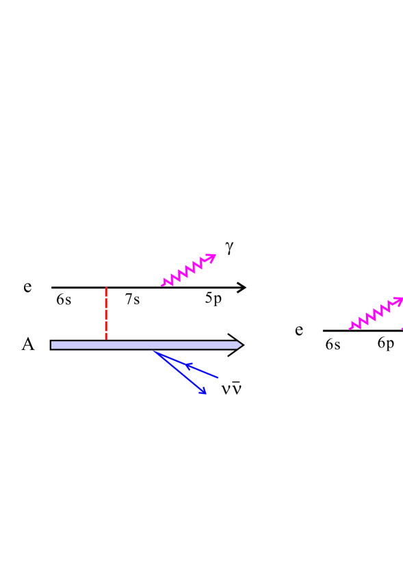
Figure 1: A part of Feynman diagrams for Xe ${}^{3}P_{1}(8.437{\rm eV})$ RENP in the left and for McQ3 in the right. Dashed red line in the left is for Coulomb excitation between nucleus A and a valence electron.

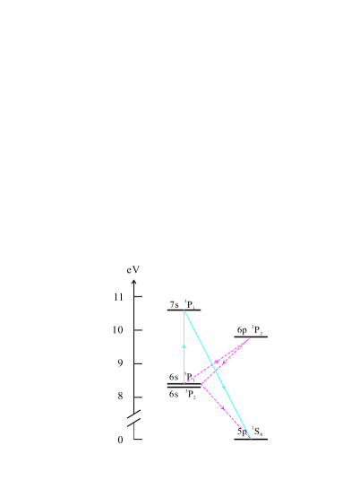
Figure 2: Relevant Xe energy levels: $|e\rangle=6s^{3}P_{1}\,,|g\rangle=5p^{1}\!S_{0}\,,|q\rangle=7s^{3}P_{1}$ ($6s^{3}P_{2}$ is for the spin current contribution in Appendix). Solid blue lines are the route for RENP, while dashed red lines are for McQ3.

The rest of this paper is organized as follows. In Section 2 the main background source of QED processes, McQ3, is discussed in detail and its rate is given along with some features of background events. Results are presented for the Xe de-excitation and the necessity of all QED background rejection is emphasized. In Section 3 we point out the possibility of the QED background rejection in targets hosted in wave guides or photonic crystals, and derive a condition for the background rejection in RENP. The idea is based on the difference of the very nature of freely propagating neutrino and restricted propagating light field in the hosted target. The background-free RENP spectrum is approximately found to be the shifted spectrum in free space, the shifted threshold being determined by the frequency cutoff in host guide. A few examples of the shifted spectrum due to the nuclear monopole contribution [10] are shown taking a few choices of the size of host guides. In the first Appendix some rudimentary facts on propagating modes in wave guides and photonic-crystal fibers are explained. The second Appendix presents the modified RENP spectrum from $6s^{3}P_{2}$ (8.315 eV) due to the spin current contribution [11].

Throughout this paper, we shall use the natural unit of $\hbar=c=1$. Conversion factors are thus $(1{\rm eV})^{-1}=1.97\times 10^{-5}{\rm cm}=(\frac{3}{1.97}\times 10^{15}{\rm Hz})^{-1}$.

2 McQ3 rate

We shall first demonstrate that without an experimental method of background rejection McQ3 process gives an enormous background rate when the process is macro-coherently amplified. Thus, it becomes a necessity to invent the rejection method when one wants to detect RENP.

Kinematics

For a fixed trigger frequency $\omega_{0}$ (of less than $\epsilon_{eg}/2$, with $\epsilon_{eg}$ the level spacing, as a necessary condition for the macro-coherence), there is a unique relation between the detected photon energy $\omega_{i}$ and its emitted angle $\theta_{i}$:

$$\cos\theta_{i}=\frac{\epsilon_{eg}}{\omega_{0}}-1-\frac{\epsilon_{eg}(\epsilon_{eg}-2\omega_{0})}{2\omega_{0}\omega_{i}}\,,\hskip 8.5359pti=1,2\,.$$ (1)

This relation may be derived from the 4-vector relation of $a-k_{0}=-(k_{1}+k_{2})$ where $a=(\epsilon_{eg},\vec{0})$ is the energy-momentum 4-vector relevant to atomic transition (the difference between the initial and the final states), and $k_{i},i=0,1,2$ are those of three photons. Note that with the macro-coherence amplification both of the energy and the momentum are conserved in the atomic process [3]. The angular constraint $|\cos\theta_{i}|\leq 1$ gives $\>\frac{\epsilon_{eg}}{2}-\omega_{0}\leq\omega_{i}\leq\frac{\epsilon_{eg}}{2}\,.\>$

Basic ¹³¹Xe data: 6s³P₁(8.437 eV) de-excitation

The initial metastable state $|e\rangle$ is an electron-hole system consisting of a valence electron of 6s and a hole of 5p or a filled state 5p⁵, their quantum numbers being much like those of two valence electron system. Relevant energy levels used are

$$|e\rangle=6s^{3}P_{1}(8.437{\rm eV})\,,\hskip 14.22636pt|p\rangle=6p^{3}P_{2}(9.821{\rm eV})\,,$$ (2)

$$|q\rangle=|e\rangle\,,\hskip 14.22636pt|g\rangle=5p^{1}S_{0}(0\,{\rm eV})\,.$$ (3)

We have used the notation of $LS$ coupling scheme, although other coupling scheme may be more appropriate for Xe. Two decay rates or A-coefficients for McQ3 rate computation are known:

$$A(6s\rightarrow 5p)\;({\rm of}\;|q\rangle\rightarrow|g\rangle)=2.81\times 10^{8}{\rm Hz}\,,\hskip 14.22636ptA(6p\rightarrow 6s)\;({\rm of}\;|p\rangle\rightarrow|q\rangle)=2.24\times 10^{7}{\rm Hz}\,.$$ (4)

McQ3 rate in free space

We need two more atomic levels in addition to $|e\rangle,|g\rangle$, to induce McQ3: they are denoted by $|p\rangle,|q\rangle$. These levels are connected to each other by electric dipole transitions of moments, $d_{ep},d_{pg},d_{qg}$. Quantum mechanical amplitude of McQ3 for a single route via virtual levels $|e\rangle\rightarrow|p\rangle\rightarrow|q\rangle\rightarrow|g\rangle$ is in proportion to

$$\vec{d}_{ep}\cdot\vec{E}_{a}\vec{d}_{pq}\cdot\vec{E}_{b}\vec{d}_{qg}\cdot\vec{E}_{c}\,,$$ (5)

where $a,b,c$ are taken respectively from (0,1,2). The magnitudes of dipole moments may be replaced by A-coefficient divided by the third power of their level spacings, hence in principle measured data can be used.

In the example of Xe de-excitation, three photon emission occurs in the third order of QED:

$$(6s5p^{-})_{J=1}\rightarrow(6p5p^{-})_{J=2}+\gamma\rightarrow(6s5p^{-})_{J=1}+\gamma+\gamma\rightarrow(5p^{2})_{J=0}+\gamma+\gamma+\gamma\,,$$ (6)

where $5p^{-}$ denotes a hole in $5p$ state. The final state denoted by $5p^{2}$ is actually the completely filled six $5p$ states 5p⁶. Three emitted photons here are taken from $\gamma_{0},\gamma_{1},\gamma_{2}$, hence there are 3! = 6 diagramatic contributions.

The differential McQ3 spectrum for a single detected photon of energy $\omega=\omega_{1}$ summed over polarizations is calculated as [12]

$$\frac{d\Gamma_{3}}{d\omega}=\frac{3\pi^{2}}{2}\frac{\gamma_{pe}\gamma_{pq}\gamma_{qg}}{\epsilon_{pe}^{3}\epsilon_{pq}^{3}\epsilon_{qg}^{3}}n^{3}V\eta_{3}(t)\omega^{2}(\epsilon_{eg}-\omega_{0}-\omega)^{2}F_{3}^{2}(\omega)\,,$$ (7)

$$F_{3}(\omega)=\frac{1}{\epsilon_{pe}+\omega_{0}}(\frac{1}{\epsilon_{qe}+\omega_{0}+\omega}+\frac{1}{\epsilon_{qg}-\omega})+\frac{1}{\epsilon_{pe}+\omega}(\frac{1}{\epsilon_{qe}+\omega_{0}+\omega}+\frac{1}{\epsilon_{qg}-\omega_{0}})$$

$$+\frac{1}{\epsilon_{pg}-\omega_{0}-\omega}(\frac{1}{\epsilon_{qg}-\omega}+\frac{1}{\epsilon_{qg}-\omega_{0}})\,.$$ (8)

The spectrum shapes are illustrated for two choices of $\omega_{0}$ taken close to $\epsilon_{eg}/2$; at $\epsilon_{eg}/2$ and its 5% reduced energy in Fig(3). Despite of a non-trivial matrix element $\propto F_{3}(\omega)$, the spectrum shape is symmetric around the point $\omega=(\epsilon_{eg}-\omega_{0})/2$. This McQ3 rate is expected much larger than the RENP rate given below.

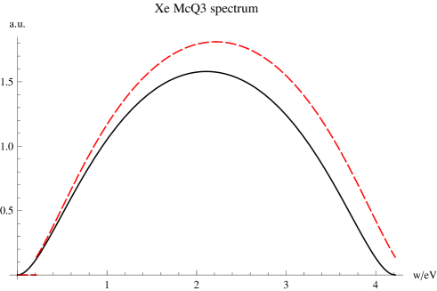
Figure 3: Xe McQ3 spectrum rate in arbitrary unit. The actual rate values integrated over photon energies are $(5\,,6)\times 10^{19}$Hz $(n/10^{20}{\rm cm}^{-3})^{3}(V/{\rm cm}^{3})(\eta_{3}(t)/10^{-3})$ for these two cases of the trigger energy $\omega_{0}$: $\omega_{0}=\epsilon_{eg}/2$ in solid black and 5% reduced value in dashed red.

It is important to mention that McQn processes, in particular, the McQ3 case has an interesting potentiality of creating a quantum entangled pair of photons under the influence of the trigger, although this is not the appropriate place to discuss the subject in detail

McQ3 in wave guide

Although photonic-crystal fibers such as the Bragg fiber [8] are more promising due to their smaller transverse sizes and other reasons, we shall explain our ideas using the wave guide because concepts are simpler there. A good comparison of these two materials is given in [7], in particular in its chapter 9.

As explained in Appendix, propagation of light field in wave guide is restricted: compared to propagation in free space, allowed modes in wave guides have discretized transverse wave vectors, $\vec{k}_{\perp}$, and their smallest cutoff.

Due to this restriction, the continuous momentum integration over 3-vector $\vec{k}$, is replaced by a semi-discrete sum. In the square wave guide of size $d$ these discrete modes are given by wave vectors in two dimensions,

$$\vec{k}_{\perp}=\frac{\pi}{d}(n_{1},n_{2})\,,\hskip 14.22636ptn_{i}=0,1,2,\cdots\,,\hskip 14.22636pt\sqrt{n_{1}^{2}+n_{2}^{2}}\geq 1\,.$$ (9)

The discrete sum over transverse momentum components may however be approximated, , when $d\epsilon_{eg}\gg 1$, by a formula of the continuous momentum integration, however with the important difference in the presence of the transverse cutoff at $k_{c}=\pi/d$.

3 Background-free RENP rate

Effective cutoff in host guides

The dispersion relation between the energy $\omega$ and the longitudinal momentum $k_{\parallel}$ along the propagation axis is given by $\omega=\sqrt{k_{\parallel}^{2}+M^{2}}$ in host guides. In the case of square wave guide of size $d$ the effective mass $M$ is discretized as $M=\sqrt{n_{1}^{2}+n_{2}^{2}}\,k_{c}\,,k_{c}=\pi/d$ with $n_{i}$ integers, as explained in Appendix. A similar effective mass exists in Bragg fibers along with the band gap [8]. It is important to note that the effective mass $M$ cannot vanish.

A derivation of the condition for the QED background rejection in RENP is given for the general case of McQn (n $\geq 3$). We use the Lorentz invariance of $A_{0}^{2}-A_{z}^{2}$ in the temporal and the spatial components of 4-vector $A$, ($A_{0},A_{z}$), where z-axis is taken along the propagation direction. We use the energy-momentum conservation: $a-k_{0}=-k-\sum_{i=2}^{n-1}k_{i}$, to give a scalar invariant relation among 2-vectors,

$$(a-k_{0})^{2}=(k+\sum_{i=2}^{n-1}k_{i})^{2}\,.$$ (10)

The invariant left hand side (LHS) quantity may be evaluated in the laboratory frame, to give $\epsilon_{eg}^{2}-2\omega_{0}\epsilon_{eg}+M_{0}^{2}$, while the right hand side (RHS) quantity is calculated in the CM system of $n-1$ longitudinal momenta, to give $(\omega+\sum_{i=2}^{n-1}\sqrt{k_{i,z}^{2}+M_{i}^{2}})^{2}$. Hence,

$$\epsilon_{eg}^{2}-2\omega_{0}\epsilon_{eg}+M_{0}^{2}=(\omega+\sum_{i=2}^{n-1}\sqrt{k_{i,z}^{2}+M_{i}^{2}})^{2}\,.$$ (11)

For the largest $\omega_{0}$ value of allowed region, one takes the smallest of RHS, namely $n-2$ photon’s transverse masses set at the fundamental mode, $M_{i}=k_{c},i=2\sim n-1$. The result is expressed by the inequality,

$$\omega_{0}\leq\frac{\epsilon_{eg}}{2}-\frac{1}{2\epsilon_{eg}}\left((\omega+(n-2)k_{c})^{2}-M_{0}^{2}\right)\,.$$ (12)

We may define the largest McQ3 trigger energy $\omega_{c}$ by taking $n=3,\omega=k_{c}$,

$$\omega_{c}=\frac{\epsilon_{eg}}{2}-\frac{1}{2\epsilon_{eg}}\left(4k_{c}^{2}-M_{0}^{2}\right)\,.$$ (13)

The trigger effective mass $M_{0}$ is often taken to be $k_{c}$ in the present work.

On the other hand, a massive neutrino of mass $m$ satisfies the dispersion relation of the energy and the momentum, $E=\sqrt{p_{z}^{2}+\vec{p}_{\perp}^{2}+m^{2}}$. A big difference is in transverse components: the neutrino transverse momentum may vanish: $\vec{p}_{\perp}=0$. This gives an allowed region for RENP;

$$\omega_{0}\leq\frac{\epsilon_{eg}}{2}-\frac{1}{2\epsilon_{eg}}\left(4m^{2}-M_{0}^{2}\right)\,.$$ (14)

RENP thresholds of neutrino pair production of mass $m_{i}$ start at

$$\omega_{ii}^{\prime}=\omega_{ii}+\frac{M_{0}^{2}}{2\epsilon_{eg}}\,,\hskip 14.22636pt\omega_{ii}=\frac{\epsilon_{eg}}{2}-\frac{2m_{i}^{2}}{\epsilon_{eg}}\,.$$ (15)

This location $\omega_{ii}^{\prime}$ is shifted to the higher energy side by an amount $M_{0}^{2}/(2\epsilon_{eg})$ from the free space value $\omega_{ii}$. $M_{0}=k_{c}$ for the trigger fundamental mode.

In both of inequalities, eq.(12) and eq.(14), the special cases of equalities give the boundary curves of two allowed regions. Thus, there exists a gap between RENP allowed regions and McQn allowed regions, if

$$(n-1)k_{c}>2m_{0}\,,\hskip 14.22636ptn\geq 3\,,$$ (16)

where $m_{0}$ is the smallest neutrino mass. The extra $k_{c}$ factor here arises from the smallest energy of $\omega$ equal to $k_{c}$. In the gap region RENP is QED background-free. The argument breaks down at $n=2$, where the usual relation $\omega=\omega_{0}=\epsilon_{eg}/2+k_{c}^{2}/(2\epsilon_{eg})$ holds [13].

Thus, all QED backgrounds are rejected once it is rejected at the smallest n value equal to 3. We illustrated the background-free region in Fig(4).

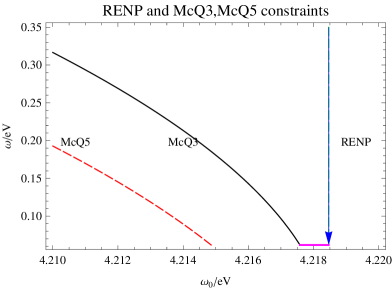
Figure 4: QED background-free regions of Xe RENP in $(\omega_{0},\omega)$ plane. Two curves give upper boundaries of McQn (n=3 in solid black, =5 in dashed red) allowed regions. Boundaries are given for the fundamental mode ($n_{1}^{2}+n_{2}^{2}=1$) and those for excited modes (not shown here) are all within these allowed regions. The background-free RENP is possible in the indicated horizontal $\omega_{0}-$region in red up to the arrow point. Assumed parameters are $\epsilon_{eg}=$8.315 eV, and the size $d=10\mu$m of photonic-crystal fiber.

RENP rates

We consider RENP from 6s${}^{3}P_{1}$(8.437 eV) [14]. We need data of 7s³P₁(10.593 eV), and its A-coefficient, $A(7s\rightarrow 5p)=8.51\times 10^{7}$s^-1, since the Coulomb excitation bridging between the nucleus and the valence electron requires another state of the same quantum number $J^{P}$ of 6s${}^{3}P_{1}$. See [10] for more details. Xe RENP rate from the nuclear pair emission, both in free space and in host guides (assuming the trigger field to be an allowed propagating mode), is given by

$$\Gamma_{\gamma 2\nu}(\omega;\,t)=\Gamma_{0}F_{X}^{2}(\omega)I(\omega)\eta_{\omega}(t)\,,$$ (17)

$$\Gamma_{0}\sim 54{\rm mHz}\frac{\epsilon_{eg}}{{\rm eV}}(\frac{n}{10^{21}{\rm cm}^{-3}})^{3}\frac{V}{10^{2}{\rm cm}^{3}}(\frac{100{\rm MHz}}{{\rm eV}^{3}})^{-1}\,.$$ (18)

$$I(\omega)=\sum_{i}\Delta_{i}(\omega)I_{i}(\omega)\theta(\omega_{ii}-\omega)\,,\hskip 14.22636pt\omega_{ii}=\frac{\epsilon_{eg}}{2}-\frac{2m_{i}^{2}}{\epsilon_{eg}}\,,$$ (19)

$$I_{i}(\omega)=\frac{\omega^{2}}{3}+\frac{2m_{i}^{2}\omega^{2}}{3\epsilon_{eg}(\epsilon_{eg}-2\omega)}+m_{i}^{2}(1+\delta_{M})\,,\hskip 14.22636pt\Delta_{i}(\omega)=\left(1-\frac{4m_{i}^{2}}{\epsilon_{eg}(\epsilon_{eg}-2\omega)}\right)^{1/2}\,,$$ (20)

$$F_{X}(\omega)=\frac{Q_{w}J_{N}(\epsilon_{7s}-\epsilon_{6s})}{\epsilon_{7s}-\epsilon_{5p}}\frac{1}{\sqrt{3\pi}}\frac{d_{7s5p}}{(\epsilon_{7s}-\epsilon_{6s}+\omega)(\epsilon_{6s}-\epsilon_{5p}-\omega)}\,,$$ (21)

where $\delta_{M}=1$ for the Majorana neutrino and $\delta_{M}=0$ for the Dirac neutrino [4].

Both in wave guides and photonic crystals, overlapping integrals containing mode functions need to be evaluated. They typically take the form,

$$I=\int_{0}^{d}dx\cos\frac{n_{x}\pi x}{d}e^{-iP_{x}x}\int_{0}^{d}dy\sin\frac{n_{y}\pi y}{d}e^{-iP_{y}y}\,,$$ (22)

for TE modes. Here $P_{i}$’s are transverse components of momentum of the neutrino pair. Let us restrict the trigger to the fundamental TE₀₁ mode: $n_{1}=0,n_{2}=1$. An elementary calculation gives

$$|I|^{2}=16(\frac{\sin(P_{x}d/2)}{P_{x}})^{2}(\frac{P_{y}\cos(P_{y}d/2)}{(\pi/d)^{2}-P_{y}^{2}})^{2}\,,\hskip 14.22636ptP_{x,y}=p_{x,y}^{1}+p_{x,y}^{2}\,.$$ (23)

In the large size limit of $d\rightarrow\infty$, the functions here are all reduced to the delta functions,

$$|I|^{2}\rightarrow 2(2\pi)^{2}d^{2}\delta(P_{x})\left(\delta(P_{y}-\frac{\pi}{d})+\delta(P_{y}+\frac{\pi}{d})\right)\,.$$ (24)

The back to back momentum balance of transverse momenta $(\vec{p}_{\perp})_{i}$ of the neutrino pair is broken by an amount, $\pm\pi\vec{n}_{0}/d$ according to this formula. Thus, the spectrum rate calculated from these delta functions coincides with the continuum limit calculation done as if the trigger were slightly off-axis. Since the squared matrix element of RENP is a smooth of the transverse momentum around $\vec{P}_{\perp}=0$, the approximation of large size limit, $d\rightarrow\infty$, is justified.

As is evident in the contour map for the background-free region, all $\omega_{0}-$region of $\omega_{0}>\omega_{c}$ ($\omega_{c}$ defined by (13) ) for RENP belongs to the McQn (n $\geq$ 3) background-free region. The background-free RENP spectrum consists of a portion of the RENP spectrum truncated at $\omega_{c}<\omega_{0}<\omega_{00}^{\prime}$, with $\omega_{00}^{\prime}$ determined by eq.(15) taking the smallest neutrino mass $m_{0}$. The full spectrum in the background-free region is shown in Fig(5).

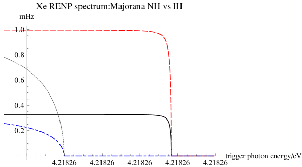
Figure 5: Xe spectral rate in the background-free region for the Majorana cases of the smallest mass, $m_{0}=$ 1 and 5 meV, and NH (in solid black and in dash-dotted blue) and IH (in dashed red and in dotted black) . Xe gas density of $1\times 10^{20}$cm^-3, the target volume $1$cm³, and $\eta_{\omega}=10^{-3}$ are assumed. The assumed size of a host guide is 100 $\mu$m.

Finally we show in Fig(6) RENP spectrum in McQn $(n\geq 2)$ background-free region, assuming $10\mu$m size of photonic-crystal fiber, to show all three thresholds $\omega_{ii}\,,i=1,2,3$ are measurable. Note that the experimental resolution of $\omega_{0}$ is made possible by the excellent frequency resolution of lasers, typically of order $10^{-7}$ eV or 100 MHz.

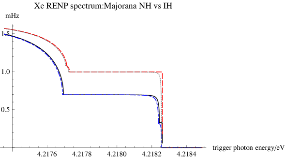
Figure 6: Xe spectral rate in the background-free region for the Majorana cases of smallest masses, 1 and 5 meV, and NH (in solid black and in dash-dotted blue) and IH (in dashed red and in dotted black). Xe gas density of $1\times 10^{20}$cm^-3, the target volume $1$cm³, and $\eta_{\omega}=10^{-3}$. The assumed size of a host guide is taken as 10 $\mu$m. Three neutrino pair emission thresholds are clearly visible.

In summary, we demonstrated that QED background-free RENP may be realized in wave guide or in some type of photonic crystals. With a large enough cutoff of transverse wave number three neutrino pair emission thresholds are detectable, using the largest nuclear monopole contribution.

We should like to thank J. Arafune for raising the QED background problem in the correct way.

4 Appendix: Propagating field modes in wave guides and photonic crystals

Allowed modes in rectangular wave guides are given by discretized transverse stationary waves. For example, the simplest TE mode propagating in z-direction have electric field components of the form [6],

$$E_{x}\propto\cos\frac{n_{x}\pi x}{a}\sin\frac{n_{y}\pi y}{b}e^{ik_{z}z}\,,\hskip 14.22636ptE_{y}\propto\sin\frac{n_{x}\pi x}{a}\cos\frac{n_{y}\pi y}{b}e^{ik_{z}z}\,,$$ (25)

with $E_{z}=0$. $n_{x},n_{y}$ are both integers. With $a<b$ the lowest fundamental modes are TE₀₁ and TM₀₁ of the eigenvalue $-\Delta_{2}=-\partial^{2}/\partial x^{2}-\partial^{2}/\partial y^{2}$ is $(\pi/b)^{2}$. For simplicity of notations we shall take the limit of a square wave guide, $a=b\equiv d$, however without further consideration of degeneracy of modes. These mode functions are orthogonal, and form a complete set for the general expansion of propagating light waves. The lowest excitation mode of TE₁₀ is given by a non-vanishing field of

$$E_{y}(x,y,z;t)=\sqrt{\frac{\omega}{V}}\sin(\frac{\pi}{d}y)e^{ik_{z}z}e^{-i\omega t}\,,\hskip 14.22636ptE_{x}(x,y,z;t)=0\,,\hskip 14.22636pt\omega=\sqrt{(\frac{\pi}{d})^{2}+k_{z}^{2}}$$ (26)

with $V=d^{2}L$ the volume of the target. The normalization of fields is determined by the condition that the energy density of this field per unit length is $\omega/L$.

Allowed projected momentum $\vec{k}_{\perp}$($=\pi(n_{x},n_{y})/d$ for TE modes) of the light field forms on a lattice given by discrete points in the projected two dimensional space orthogonal to the trigger axis, denoted in general by $\pi\vec{n}/d$. Unless the projected momentum falls on these lattice points, the photon emission is forbidden in wave guide. We may introduce an effective cutoff wave number by $k_{c}=\pi/d$: transverse momenta of $|\vec{k}_{\perp}|<k_{c}$ are forbidden in the wave guide. The important point for the background rejection is that this cutoff acts as an effective mass to parallel momentum component $k_{\parallel}$ of $\omega=\sqrt{k_{\parallel}^{2}+\vec{k}_{\perp}^{2}}$.

Eigenvalue problem in photonic crystals

We shall recapitulate basic features of eigen-modes that propagate in cylindrical fibers of photonic crystals.

First, the fundamental eigenvalue equation is set up for the magnetic field [7],

$$\vec{H}_{\vec{k}}(\vec{r})=e^{i\vec{k}\cdot\vec{r}}\vec{u}_{\vec{k}}(\vec{r})\,,\hskip 14.22636pt\vec{E}_{\vec{k}}(\vec{r})=e^{i\vec{k}\cdot\vec{r}}\frac{i}{\omega(\vec{k})\epsilon(\vec{r})}(i\vec{k}+\vec{\nabla})\times\vec{u}_{\vec{k}}(\vec{r})\,,$$ (27)

$$(i\vec{k}+\vec{\nabla})\times\frac{1}{\epsilon(\vec{r})}(i\vec{k}+\vec{\nabla})\times\vec{u}_{\vec{k}}(\vec{r})=\omega^{2}(\vec{k})\vec{u}_{\vec{k}}(\vec{r})\,,$$ (28)

where $\epsilon(\vec{r})$ is the dielectric function which may depend on spatial places. The linear operator acting the vector function $\vec{u}_{\vec{k}}(\vec{r})$ is hermitian.

In the case of cylindrical photonic-crystal fibers, one may use the cylindrical symmetry of the dielectric function $\epsilon(\vec{r})$, to factor out the cyclic coordinate dependence,

$$\vec{u}_{\vec{k}}(\vec{r})=e^{ik_{z}z+in\varphi}\vec{h}_{k_{z},n}(\rho)\,,\hskip 14.22636pt\rho=\sqrt{x^{2}+y^{2}}\,,$$ (29)

where $k_{z}$ is an arbitrary real number and $n$ is an integer. We shall not write down an ordinary differential equation for the vector function $\vec{h}_{k_{z},n}(\rho)$. This is the eigenvalue problem in one dimension (1D) due to the cylindrical symmetry.

When the eigenvalue problem is applied to a multi-layer dielectrics of alternating dielectric constants with a large-size air hole in the center [8], there exist band gaps and their dispersion relation $\omega(k_{z})$ provides the effective cutoff of order $\pi/d$, where $d$ is the cladding periodicity, the hole radius being taken comparable to $d$. Some details are shown in [9].

5 Appendix: Spin current contribution from ${}^{3}P_{2}$ (8.315 eV) de-excitation

For completeness we show in Fig(7) the spin current contribution using the formulas of [11]. Although rates are much smaller than the nuclear monopole contribution of preceding figures, this case has a potentiality to access the Majorana CPV phase determination.

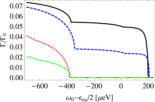
Figure 7: Xe spectral rate in the background-free region due to the spin current contribution from ${}^{3}P_{2}$(8.315 eV) in wave guide of size $d=10\mu$m. The actual rate is derived by multiplying $\Gamma_{0}\sim 9.4\times 10^{-5}$mHz for $n=10^{20}{\rm cm}^{-3},V=1{\rm cm}^{3},\eta_{\omega}=1$ of Xe target (the rate scaling like $\propto n^{3}V\eta_{\omega}$). Plotted are the Majorana cases of smallest masses, 10 and 50 meV, and NH and IH; 10 meV NH in solid black, 10 meV IH in dashed blue, 50 meV NH in dotted red, and 50 meV IH in dash-dotted green.

References

• [1] yoshim@okayama-u.ac.jp $\dagger$ sasao@okayama-u.ac.jp $\ddagger$ tanaka@phys.sci.osaka-u.ac.jp
• [2] Y. Miyamoto et al, arXiv:1406.2198v2 [physics.atom-ph] (2014) and Prog.Theor.Exp.Phys. 113C01(2014).
• [3] An intuitive way of understanding the macro-coherence is as follows. Suppose that we calculate a total rate of collective body of excited atoms given by a formula, $\>|\sum_{a}e^{i(\vec{k}+\vec{p}_{1}+\vec{p}_{2})\cdot\vec{r}_{a}}{\cal M}_{a}|^{2}\,,\>$ where emitted plane waves at atomic site $\vec{r}_{a}$ are explicitly written. If the atomic phase relaxation at different atomic sites is slow in time and atomic matrix elements ${\cal M}_{a}$ are spatially slowly varying, then one may factor out this part of matrix elements, to obtain the above formula $\>=(2\pi)^{3}\delta(\vec{k}+\vec{p}_{1}+\vec{p}_{2})n^{2}V|{\cal M}|^{2}\,,\>$ where $n$ is the number density of excited atoms in the coherent volume $V$. An extra $n$ factor in $\propto n^{3}V$ dependence of rates arises from the stored field, since the process is stimulated by the stored field.
• [4] A. Fukumi et al., Prog.Β Theor.Β Exp.Β Phys.Β (2012) 04D002, and earlier references cited therein.
• [5] M. Yoshimura, N. Sasao, and M. Tanaka, Experimental method of detecting relic neutrino by atomic de-excitation, arXiv: 1409.3648v1 (2014).
• [6] For a general introduction on wave guides, R.E. Collin, Foundations for Microwave Engineering, Wiley-Interscience (1992).
• [7] J.D. Joannopoulos, S.G. Johnson, J.N. Winn, and R.D. Meade, Photonic Crystals, second edition, Princeton University Press (2008).
• [8] P. Yeh, A. Yariv, and E. Marom, J. Opt. Soc. Am., 68, 1196(1978). The band structure of the photonic-crystal fiber is shown in [8].
• [9] Chapter 9 of [7] on photonic-crystal fibers. In particular, Figure 15 in this chapter is illuminating to understand differences of field propagation in wave guides and Bragg fibers.
• [10] M. Yoshimura and N. Sasao, Phys.Β Rev.Β D 89, 053013 (2014). There is a serious typo of statement immediately prior to eq.(17) in this paper. Canceling diagrams are the leftmost of Fig.1 and two of Fig.2 instead of the stated ones which give the result of eq.(19). All written formulas in the paper are correct. A numerical typo was further corrected.
• [11] D.N. Dinh, S. Petcov, N. Sasao, M. Tanaka, and M. Yoshimura, Phys. Lett.B719,154(2012).
• [12] Identical particle effects of bosons have been neglected in this formula.
• [13] PSR process based on two dipole transitions E1 $\times$ E1 has been discussed in M. Yoshimura, N. Sasao, and M. Tanaka, Phys.Β Rev.Β A 86, 013812 (2012), which does not contribute as RENP background when one can neglect effects of parity mixture such as a stray field in Xe de-excitation. Other types of PSR arising, for example, from M1 $\times$ E1 type involving parity change, may contribute as a background in Xe RENP. This background can be rejected if one chooses $\omega_{0}$ of RENP larger than $\epsilon_{eg}/2$, which is possible by the up-shifted neutrino pair threshold.
• [14] The scheme we consider here for RENP relies on a fast repetition cycle of back to the ground state in order not to lose RENP events in dead time. This is because the development of macro-coherence is destroyed at the phase relaxation time $T_{2}$, which is typically 1$\sim$ 10 ns in dense targets. A typical repetition cycle we may think of is of order 1$\sim$ 100 kHz, to be compared with the E1 transition rate of order 10 ns, giving an effective RENP time fraction of order $10^{-5}\sim 10^{-3}$. The effective RENP rate is reduced by this factor from those of rates in our figures. Another scheme is to use as the initial state ${}^{3}P_{2}(8.315{\rm eV})$ with a magnetic mixing of the state ${}^{3}P_{1}(8.437{\rm eV})$ (required from the selection rule of $|\Delta J|=1$ for RENP). The magnetic mixing amplitude $\delta_{m}$ is of order, $\>\delta_{m}=\mu_{B}B/\Delta\sim 5\times 10^{-5}(B/{\rm T})({\rm eV}/\Delta)\,,\>$ with $\Delta$ the energy difference between two mixed states ($0.12$eV in the Xe case, giving $\delta_{m}$ of order $5\times 10^{-2}$ for 10 T magnetic field). RENP rates are reduced by $\delta_{m}^{2}$.