Long time behavior of solutions of Fisher-KPP equation with advection and free boundaries^§

Abstract.

We consider Fisher-KPP equation with advection: $u_{t}=u_{xx}-\beta u_{x}+f(u)$ for $x\in(g(t),h(t))$, where $g(t)$ and $h(t)$ are two free boundaries satisfying Stefan conditions. This equation is used to describe the population dynamics in advective environments. We study the influence of the advection coefficient $-\beta$ on the long time behavior of the solutions. We find two parameters $c_{0}$ and $\beta^{*}$ with $\beta^{*}>c_{0}>0$ which play key roles in the dynamics, here $c_{0}$ is the minimal speed of the traveling waves of Fisher-KPP equation. More precisely, by studying a family of the initial data $\{\sigma\phi\}_{\sigma>0}$ (where $\phi$ is some compactly supported positive function), we show that, (1) in case $\beta\in(0,c_{0})$, there exists $\sigma^{*}\geqslant 0$ such that spreading happens when $\sigma>\sigma^{*}$ (i.e., $u(t,\cdot;\sigma\phi)\to 1$ locally uniformly in $\mathbb{R}$) and vanishing happens when $\sigma\in(0,\sigma^{*}]$ (i.e., $[g(t),h(t)]$ remains bounded and $u(t,\cdot;\sigma\phi)\to 0$ uniformly in $[g(t),h(t)]$); (2) in case $\beta\in(c_{0},\beta^{*})$, there exists $\sigma^{*}>0$ such that virtual spreading happens when $\sigma>\sigma^{*}$ (i.e., $u(t,\cdot;\sigma\phi)\to 0$ locally uniformly in $[g(t),\infty)$ and $u(t,\cdot+ct;\sigma\phi)\to 1$ locally uniformly in $\mathbb{R}$ for some $c>\beta-c_{0}$), vanishing happens when $\sigma\in(0,\sigma^{*})$, and in the transition case $\sigma=\sigma^{*}$, $u(t,\cdot+o(t);\sigma\phi)\to V^{*}(\cdot-(\beta-c_{0})t)$ uniformly, the latter is a traveling wave with a “big head” near the free boundary $x=(\beta-c_{0})t$ and with an infinite long “tail” on the left; (3) in case $\beta=c_{0}$, there exists $\sigma^{*}>0$ such that virtual spreading happens when $\sigma>\sigma^{*}$ and $u(t,\cdot;\sigma\phi)\to 0$ uniformly in $[g(t),h(t)]$ when $\sigma\in(0,\sigma^{*}]$; (4) in case $\beta\geqslant\beta^{*}$, vanishing happens for any solution.

1. Introduction

In this paper, we consider the following problem

($$P \left\{\begin{array}[]{ll}u_{t}=u_{xx}-\beta u_{x}+f(u),&g(t)<x<h(t),\;t>0,\\ u(t,g(t))=0,\ \ g^{\prime}(t)=-\mu u_{x}(t,g(t)),&t>0,\\ u(t,h(t))=0,\ \ h^{\prime}(t)=-\mu u_{x}(t,h(t)),&t>0,\\ -g(0)=h(0)=h_{0},\ \ u(0,x)=u_{0}(x),&-h_{0}\leqslant x\leqslant h_{0},\end{array}\right.$$)

where $\mu$ and $\beta$ are positive constants, $h_{0}>0$ and $u_{0}$ is a nonnegative $C^{2}$ function with support in $[-h_{0},h_{0}]$, $f:[0,\infty)\to\mathbb{R}$ is a $C^{1}$ function satisfying

($$F \left\{\begin{array}[]{ll}f(0)=f(1)=0,\quad(1-u)f(u)>0\mbox{ for }u>0\mbox{ and }u\not=1,\\ f^{\prime}(0)>0,\ f^{\prime}(1)<0\mbox{ and }f(u)\leqslant f^{\prime}(0)u\mbox{ for }u\geqslant 0.\end{array}\right.$$)

The problem ($P$) is used to model the spreading of a new or invasive species, under the influence of diffusion and advection. The unknown $u(t,x)$ denotes the population density over a one dimensional habitat and the free boundaries $x=g(t)$ and $x=h(t)$ represent the expanding fronts of the species. We assume that the free boundaries move according to one-phase Stefan condition, which is a kind of free boundary conditions widely used in the study of melting of ice [38], wound healing [9], and population dynamics [7, 12, 13]. The derivation of one-phase or two-phase Stefan conditions in population models as singular limits of competition-diffusion systems can be found in [26, 27] etc.

When $\beta=0$ (i.e., there is no advection in the environment), the qualitative properties of the problem ($P$) was studied by Du and Lin [12] for logistic nonlinearity $f(u)=u(1-u)$. Among others, they proved that, when $h_{0}\geqslant\frac{\pi}{2}$, any solution of ($P$) with $\beta=0$ grows up and converges to $1$ (which is called spreading phenomena); when $h_{0}<\frac{\pi}{2}$, spreading happens if $\mu$ is large and vanishing happens if $\mu$ is small (i.e., the solution converges to $0$). The vanishing phenomena is a remarkable result since it shows that the presence of free boundaries may avoid the so-called hair-trigger effect, which is a phenomena shown in [2]: spreading always happens for a solution of the Cauchy problem for $u_{t}=u_{xx}+f(u)$, no matter how small the positive initial data is. Recently, Du and Lou [13] extended the results in [12] to the problem with general monostable, bistable and combustion types of $f$, and gave a rather complete description on the long time behavior of the solutions. In addition, Kaneko and Yamada [31], Liu and Lou [32, 33] studied the problem ($P$) with $\beta=0$ and with a fixed boundary $g(t)\equiv 0$, Du and Guo [10, 11], Du, Matano and Wang [16], Zhou and Xiao [43], Wang [42] studied the problem (without advection) in higher dimension spaces and/or in spatial heterogeneous environments. Besides the qualitative properties, another interesting problem is the asymptotic spreading speeds of the free boundaries when spreading happens. Du and Lin [12], Du and Lou [13] proved that, when spreading happens for a solution $(u,g,h)$ of the problem ($P$) with $\beta=0$,

(1.1) $$c^{*}:=\lim_{t\to\infty}\frac{h(t)}{t}=\lim_{t\to\infty}\frac{-g(t)}{t}>0.$$

Recently, Du, Matsuzawa and Zhou [17] improved this result to better ones:

(1.2) $$\lim_{t\to\infty}h^{\prime}(t)=\lim_{t\to\infty}[-g^{\prime}(t)]=c^{*},\quad\lim_{t\to\infty}[h(t)-c^{*}t]=H_{\infty},\quad\lim_{t\to\infty}[g(t)+c^{*}t]=G_{\infty},$$

for some $H_{\infty},\ G_{\infty}\in\mathbb{R}$.

In this paper we consider the problem ($P$) with $\beta>0$, which means that the spreading of a species is affected by advection. In the field of ecology, organisms can often sense and respond to local environmental cues by moving towards favorable habitats, and these movement usually depend upon a combination of local biotic and abiotic factors such as stream, climate, food and predators. For example, some diseases spread along the wind direction. In 2009, Maidana and Yang [34] studied the propagation of West Nile Virus from New York City to California state. It was observed that West Nile Virus appeared for the first time in New York City in the summer of 1999. In the second year the wave front travels 187km to the north and 1100km to the south. Therefore, they took account of the advection movement and showed that bird advection becomes an important factor for lower mosquito biting rates. Another example is that Averill [3] considered the effect of intermediate advection on the dynamics of two-species competition system, and provided a concrete range of advection strength for the coexistence of two competing species. Moreover, three different kinds of transitions from small advection to large advection were illustrated theoretically and numerically. Many other examples involving advection can also be found in the field of ecology (cf. [4, 5, 8, 36, 37, 39, 40, 41] etc.).

From a mathematical point of view, to involve the influence of advection, one of the simplest but probably still realistic approaches is to assume that species can move up along the gradient of the density, as considered in [6, 28, 29, 37, 39, 40, 41] etc.

Gu, Lin and Lou [23, 24] studied the problem ($P$) with small advection. They proved a spreading-vanishing dichotomy result on the long time behavior of positive solutions of ($P$), which is similar as the conclusions in [12, 13] for equations without advection. They also proved that, when spreading happens for a solution of ($P$) with small advection, its rightward spreading speed is bigger than the leftward one:

(1.3) $$\lim_{t\to\infty}\frac{h(t)}{t}>\lim_{t\to\infty}\frac{-g(t)}{t}>0.$$

Recently, Kaneko and Matsuzawa [30] improved this result to some conclusions like (1.2).

Our main purpose in this paper is to study the influence of the advection term $-\beta u_{x}$ on the long time behavior of solutions of ($P$). As we will see below, our study improves the results in [23, 24, 30] since we will study the problem ($P$) for all $\beta>0$, not only for small $\beta$. Especially, when $\beta$ is large, the phenomena is much more complicated and more interesting than the case where $\beta$ is small.

We point that the problem ($P$) for the equations with bistable type of nonlinearity, or the problems (with monostable or bistable type of nonlinearity) in the interval $[0,h(t)]$ with $x=h(t)$ a free boundary and $x=0$ a fixed boundary where $u$ satisfies a general Robin boundary condition can be considered similarly. In fact, in our forthcoming papers [20, 21, 22] we study these problems and obtain similar results as in this paper.

To sketch the influence of $\beta$, we introduce two important traveling waves. First, consider the following problem

(1.4) $$\left\{\begin{array}[]{ll}q^{\prime\prime}(z)-cq^{\prime}(z)+f(q)=0,\quad z\in\mathbb{R},\\ q(-\infty)=0,\ q(+\infty)=1,\ q(0)=1/2,\quad q^{\prime}(z)>0\mbox{ for }z\in\mathbb{R}.\end{array}\right.$$

It is well known that this problem has a solution $q(z;c)$ if and only if $c\geqslant c_{0}$, where

$$c_{0}:=2\sqrt{f^{\prime}(0)}$$

is called the minimal speed of the traveling waves of Fisher-KPP equation. Denote $Q(z):=q(z;c_{0})$, then $u(t,x)=Q(x-(\beta-c_{0})t)$ is a traveling wave of $u_{t}=u_{xx}-\beta u_{x}+f(u)$. It travels leftward (resp. rightward) if and only if $\beta<c_{0}$ (resp. $\beta>c_{0}$). Next we consider the following problem

(1.5) $$\left\{\begin{array}[]{ll}q^{\prime\prime}(z)+(c-\beta)q^{\prime}(z)+f(q)=0,\quad z\in(-\infty,0),\\ q(0)=0,\ q(-\infty)=1,\ -\mu q^{\prime}(0)=c,\quad q^{\prime}(z)<0\mbox{ for }z\in(-\infty,0].\end{array}\right.$$

As is shown in Lemma 3.4 (see also [12, 13, 24]), for any $\beta>0$, this problem has a unique solution $(c,q)=(c^{*},U^{*}(z))$. So $u(t,x)=U^{*}(x-c^{*}t)$ is a solution of $u_{t}=u_{xx}-\beta u_{x}+f(u)$, with $u(t,c^{*}t)=0,\ c^{*}=-\mu u_{x}(t,c^{*}t)$. It is called a traveling semi-wave in [13] since it is only defined for $x\leqslant c^{*}t$. We also write $c^{*}$ as $c^{*}(\beta)$ to emphasize the dependence of $c^{*}$ on $\beta$, then we will show in Lemma 3.4 that the equation $\beta-c_{0}=c^{*}(\beta)$ has a unique root $\beta^{*}>c_{0}$:

(1.6) $$\beta^{*}-c_{0}=c^{*}(\beta^{*}).$$

We will see below that the traveling wave $Q(x-(\beta-c_{0})t)$ and the traveling semi-wave $U^{*}(x-c^{*}t)$ are of special importance in the study of spreading solutions. To explain their roles intuitively, we consider the problem ($P$) with initial data $u_{0}(x)$ which is even and

$$u_{0}(x)=\left\{\begin{array}[]{ll}1,&x\in[0,h_{0}-1],\\ \mbox{smooth and decreasing},&x\in[h_{0}-1,h_{0}],\end{array}\right.\qquad\mbox{ with }h_{0}\gg 1.$$

It is easily seen by the maximum principle that $u(t,\cdot)$ has exactly one maximum point. As usual, we call the sharp decreasing part in the graph of $u(t,\cdot)$ the front, and call the sharp increasing part on the left side the back. Now we sketch the influence of the advection $-\beta u_{x}$. Case 1. When $\beta\in(0,c_{0})$, the advection influence is not strong, the solution has enough space between the back and the front to grow up and to converge to 1. Its front approaches a profile like $U^{*}(\cdot)$ and moves rightward at a speed $\approx c^{*}$. Its back approaches a profile like $U^{*}(-\;\cdot)$ and moves leftward at a speed smaller than $c_{0}-\beta$ (see details in Theorem 2.5 below). This case is similar as the spreading phenomena in [12, 13] for the equation with $\beta=0$. Case 2. When $\beta\in(c_{0},\beta^{*})$ with $\beta^{*}$ being the unique root of (1.6), the traveling wave $Q(x-(\beta-c_{0})t)$ travels rightward at a speed $\beta-c_{0}>0$. Hence the back of the solution $u$, with a shape like $Q(x-(\beta-c_{0})t)$, is pushed by $Q(x-(\beta-c_{0})t)$ to move rightward at a speed $\approx\beta-c_{0}$, and so $u\to 0$ locally uniformly. But, when the initial domain is wide enough, the solution still have enough space to grow up between the back and the front since the front moves rightward (at a speed $\approx c^{*}$) faster than the back. In this paper we call such a phenomena as virtual spreading (see Theorem 2.2 and Lemma 4.11 below). Case 3. When $\beta=c_{0}$, the traveling wave $Q(x-(\beta-c_{0})t)=Q(x)$ is indeed a stationary solution of ($P$)₁. However, the back of the solution $u$ still moves rightward at a speed $O(t^{-1})$ since it starts from a compactly supported initial data $u_{0}$ (cf. [25] and see details below). Hence virtual spreading still happens when $h_{0}$ is sufficiently large, since the front moves rightward at speed $c^{*}$, faster than the back. Case 4. When $\beta>\beta^{*}$, the back moves rightward (at a speed $\approx\beta-c_{0}$) faster than the front (which moves rightward at speed $\approx c^{*}<\beta-c_{0}$). So the solution is suppressed by its back, and then $u\to 0$ uniformly. In summary, the long time behavior of the solutions is quite different for $\beta\in(0,c_{0}),\;\beta=c_{0},\;\beta\in(c_{0},\beta^{*})$ and $\beta>\beta^{*}$.

This paper is organized as the following. In section 2 we present our main results. In section 3 we give some preliminaries including the comparison principles, stationary solutions, several types of traveling waves, zero number arguments and some upper bound estimates. In section 4 we study the influence of the advection on the long time behavior of the solutions. In section 5, we revisit the virtual spreading phenomena and give a uniform convergence for such solutions.

2. Main Results

Throughout this paper we choose initial data $u_{0}$ from the following set:

(2.1) $$\mathscr{X}(h_{0}):=\Big{\{}\phi\in C^{2}([-h_{0},h_{0}])\mid\phi(-h_{0})=\phi(h_{0})=0,\;\phi(x)\geqslant,\not\equiv 0\ \mbox{in }(-h_{0},h_{0}).\Big{\}}$$

where $h_{0}>0$ is any given real number. By a similar argument as in [12, 13], one can show that, for any initial data $u_{0}\in\mathscr{X}(h_{0})$, the problem ($P$) has a time-global solution $(u,g,h)$, with $u\in C^{1+\nu/2,2+\nu}((0,\infty)\times[g(t),h(t)])$ and $g,h\in C^{1+\nu/2}((0,\infty))$ for any $\nu\in(0,1)$. Moreover, it follows from the maximum principle that, when $t>0$, the solution $u$ is positive in $(g(t),h(t))$, $u_{x}(t,g(t))>0$ and $u_{x}(t,h(t))<0$. Hence $g^{\prime}(t)<0$, $h^{\prime}(t)>0$. Denote

$$g_{\infty}:=\lim_{t\to\infty}g(t),\quad h_{\infty}:=\lim_{t\to\infty}h(t),\quad I(t):=[g(t),h(t)]\quad\mbox{and}\quad I_{\infty}:=(g_{\infty},h_{\infty}).$$

In what follows, we mainly consider the solution of ($P$) with initial data $u_{0}=\sigma\phi$ for some given $\phi\in\mathscr{X}(h_{0})$ and $\sigma\geqslant 0$. We also use $(u(t,x;\sigma\phi),g(t;\sigma\phi),h(t;\sigma\phi))$ to denote such a solution. Now we list some possible situations for the solutions of ($P$).

• spreading : $I_{\infty}=\mathbb{R}$ and

  (2.2) $$\lim_{t\to\infty}u(t,\cdot)=1\mbox{ locally uniformly in $\mathbb{R}$};$$

• vanishing : $I_{\infty}$ is a bounded interval and

  (2.3) $$\lim_{t\to\infty}\max_{g(t)\leqslant x\leqslant h(t)}u(t,x)=0;$$

• virtual spreading : $g_{\infty}>-\infty,\ h_{\infty}=+\infty$,

  (2.4) $$\lim_{t\to\infty}u(t,\cdot)=0\mbox{ locally uniformly in }I_{\infty}$$

  and

  (2.5) $$\lim_{t\to\infty}u(t,\cdot+ct)=1\mbox{ locally uniformly in }\mathbb{R},\quad\mbox{ for some }c>0;$$

• virtual vanishing : $g_{\infty}>-\infty,\ h_{\infty}=+\infty$ and (2.3) holds.

When the advection is small, we have the following conclusion on the long time behavior of the solutions.

Theorem 2.1 (the case $\beta\in(0,c_{0})$).

Assume $0<\beta<c_{0}$ and $(u,g,h)$ is a time-global solution of ($P$) with initial data $u_{0}=\sigma\phi$ for some $\phi\in\mathscr{X}(h_{0})$. Then there exists $\sigma^{*}=\sigma^{*}(h_{0},\phi)\in[0,\infty]$ such that

(i) vanishing happens when $\sigma\in[0,\sigma^{*}]$, with $|I_{\infty}|=h_{\infty}-g_{\infty}\leqslant\frac{2\pi}{\sqrt{c_{0}^{2}-\beta^{2}}}$;

(ii) spreading happens when $\sigma>\sigma^{*}$.

From this theorem we see that the long time behavior of the solutions of ($P$) with small advection: $\beta\in(0,c_{0})$ is similar as the case without advection: $\beta=0$ (cf. [12, 13, 23]). The main reason is that in both cases the problem ($P$) has exactly two stationary solutions: $0$ and $1$ in $\mathbb{R}$. The proof of this theorem, which is given in subsection 4.2, is also similar as that for $\beta=0$.

Next we consider the case where the advection is not small: $\beta\geqslant c_{0}$. The most interesting phenomena appears in the problem with medium-sized advection: $\beta\in[c_{0},\beta^{*})$, where $\beta^{*}$ is the unique root of (1.6).

Theorem 2.2 (the case $c_{0}<\beta<\beta^{*}$).

Assume $c_{0}<\beta<\beta^{*}$ and $(u,g,h)$ is a time-global solution of ($P$) with initial data $u_{0}=\sigma\phi$ for some $\phi\in\mathscr{X}(h_{0})$. Then there exists $\sigma^{*}=\sigma^{*}(h_{0},\phi)\in(0,\infty]$ such that

(i) virtual spreading happens when $\sigma>\sigma^{*}$, and

$$\lim_{t\to\infty}u(t,\cdot+ct)=1\mbox{ locally uniformly in $\mathbb{R}$},\quad\mbox{ for any }c\in(\beta-c_{0},c^{*}),$$

where $c^{*}=c^{*}(\beta)$ is the speed of the traveling semi-wave in (1.5);

(ii) vanishing happens when $0<\sigma<\sigma^{*}$;

(iii) in the transition case $\sigma=\sigma^{*}$: $g_{\infty}>-\infty,\ h_{\infty}=+\infty$,

$$\lim_{t\to\infty}h^{\prime}(t)=\beta-c_{0}\quad\mbox{and}\quad h(t)=(\beta-c_{0})t+\varrho(t)$$

with $\varrho(t)=o(t)$ and $\varrho(t)\to\infty\ (t\to\infty)$. In addition,

(2.6) $$\lim\limits_{t\to\infty}\|u(t,\cdot)-V^{*}(\cdot-(\beta-c_{0})t-\varrho(t))\|_{L^{\infty}(I(t))}=0,$$

where $V^{*}(z)$ is the unique solution of

(2.7) $$\left\{\begin{array}[]{ll}q^{\prime\prime}(z)-c_{0}q^{\prime}(z)+f(q)=0\quad\mbox{for }z\in(-\infty,0),\\ q(0)=0,\ q(-\infty)=0,\ q(z)>0\mbox{ for }z\in(-\infty,0),\ -\mu q^{\prime}(0)=\beta-c_{0}.\end{array}\right.$$

In the next section we will see that $V^{*}$ has a tadpole-like shape: it has a “big head” and a boundary on the right side and an infinite long “tail” on the left side. So we call $V^{*}(x-(\beta-c_{0})t)$ a tadpole-like traveling wave with speed $\beta-c_{0}$, which exists if and only if $\beta\in(c_{0},\beta^{*})$ (see Lemma 3.5 below). Theorem 2.2 (iii) implies that, roughly, $u(t,x)$ converges to this traveling wave.

In Aronson and Weinberger [2], it was shown that any positive solution of the Cauchy problem for Fisher-KPP equation converges to 1 (i.e., hair-trigger effect). In [12, 13], by introducing the free boundaries, the authors proved a spreading-vanishing dichotomy on the long time behavior of the solutions of Fisher-KPP equation. In particular, vanishing may happen for some solutions. Now our Theorem 2.2 gives the third possibility besides the virtual spreading and vanishing, that is, with a medium-sized advection in the equation, there may exist a transition state: the solution converges to a tadpole-like traveling wave. This interesting phenomena is new comparing with the results for Cauchy problems and for free boundary problems without advection.

Theorem 2.3 (the case $\beta=c_{0}$).

Assume $\beta=c_{0}$ and $(u,g,h)$ is a time-global solution of ($P$) with initial data $u_{0}=\sigma\phi$ for some $\phi\in\mathscr{X}(h_{0})$. Then there exists $\sigma_{*},\;\sigma^{*}\in(0,\infty]$ with $\sigma_{*}\leqslant\sigma^{*}$ such that

(i) virtual spreading happens when $\sigma>\sigma^{*}$, and

$$\lim_{t\to\infty}u(t,\cdot+ct)=1\mbox{ locally uniformly in $\mathbb{R}$},\quad\mbox{ for any }c\in(0,c^{*}),$$

where $c^{*}=c^{*}(\beta)$ is the speed of the traveling semi-wave in (1.5);

(ii) vanishing happens when $0<\sigma<\sigma_{*}$;

(iii) virtual vanishing happens when $\sigma\in[\sigma_{*},\sigma^{*}]$.

The transition cases in Theorem 2.2 and Theorem 2.3 are different. In case $c_{0}<\beta<\beta^{*}$, a solution $u(t,x;\sigma\phi)$ is a transition one only if the initial value is taken the sharp threshold value $\sigma^{*}\phi$. However, in case $\beta=c_{0}$, we obtain transition solutions whose initial data are taken from $\{\sigma\phi\mid\sigma\in[\sigma_{*},\sigma^{*}]\}$. Whether or not this domain is a singleton: $\sigma_{*}=\sigma^{*}$ is still open now. The difficulty in studying this problem is that virtual vanishing solutions have no “shapes”, so it is not easy to compare one to another.

The conclusions for the problem with large advection: $\beta\geqslant\beta^{*}$ is rather simple.

Theorem 2.4 (the case $\beta\geqslant\beta^{*}$).

Assume $\beta\geqslant\beta^{*}$ and $(u,g,h)$ is a time-global solution of ($P$) with initial data $u_{0}\in\mathscr{X}(h_{0})$. Then vanishing happens.

Besides the convergence/dichotomy/trichotomy results on the long time behavior of the solutions as stated in the previous theorems, we can say more about the solutions when (virtual) spreading happens. It turns out that, when $\beta\in[c_{0},\beta^{*})$, the virtual spreading solution can be characterized by the rightward traveling semi-wave $U^{*}(x-c^{*}t)$ and the traveling wave $Q(x-(\beta-c_{0})t)$; when $\beta\in(0,c_{0})$, the spreading solution can be characterized by $U^{*}(x-c^{*}t)$ and the leftward traveling semi-wave $U^{*}_{l}(x-c^{*}_{l}t)$. Here $(c^{*}_{l},U^{*}_{l})$ (with $c_{l}^{*}<0$) is the unique solution of the following problem with $\beta\in(0,c_{0})$ (see details in subsection 3.3)

(2.8) $$\left\{\begin{array}[]{ll}q^{\prime\prime}(z)+(c-\beta)q^{\prime}(z)+f(q)=0,\quad z\in(0,\infty),\\ q(0)=0,\ q(\infty)=1,\ -\mu q^{\prime}(0)=c,\ q^{\prime}(z)>0\mbox{ for }z\in(0,\infty).\end{array}\right.$$

Using these traveling waves we can give the asymptotic profiles for (virtual) spreading solutions.

Theorem 2.5.

Assume spreading or virtual spreading happens for a solution of ($P$) as in Theorems 2.1, 2.2 or 2.3. Let $(c^{*},U^{*})$ be the unique solution of (1.5) with $c^{*}>0$.

• When $\beta\in(0,c_{0})$, let $(c_{l}^{*},U_{l}^{*})$ be the unique solution of (2.8) with $0<-c_{l}^{*}<c^{*}$. Then there exist $H_{\infty}$, $G_{\infty}\in\mathbb{R}$ such that

  (2.9) $$\lim\limits_{t\to\infty}[h(t)-c^{*}t]=H_{\infty},\quad\lim\limits_{t\to\infty}h^{\prime}(t)=c^{*},$$

  (2.10) $$\lim\limits_{t\to\infty}[g(t)-c_{l}^{*}t]=G_{\infty},\quad\lim\limits_{t\to\infty}g^{\prime}(t)=c_{l}^{*},$$

  and, if we extend $U^{*}$, $U_{l}^{*}$ to be zero outside their supports we have

  (2.11) $$\lim\limits_{t\to\infty}\left\|u(t,\cdot)-U^{*}(\cdot-c^{*}t-H_{\infty})\cdot U^{*}_{l}\big{(}\cdot-c^{*}_{l}t-G_{\infty}\big{)}\right\|_{L^{\infty}(I(t))}=0.$$

• When $\beta\in[c_{0},\beta^{*})$, (2.9) holds for some $H_{\infty}\in\mathbb{R}$. Moreover, if we extend $U^{*}$ to be zero outside its support, then

  (2.12) $$\lim\limits_{t\to\infty}\left\|u(t,\cdot)-U^{*}(\cdot-c^{*}t-H_{\infty})\cdot Q\big{(}\cdot-(\beta-c_{0})t-\theta(t)\big{)}\right\|_{L^{\infty}(I(t))}=0$$

  for some function $\theta(t)$ satisfying $\theta(t)=o(t)$ and $\theta(t)\to\infty\ (t\to\infty)$.

Assume $\beta\in[0,c_{0})$ and spreading happens for a solution $(u,g,h)$ of ($P$). The asymptotic spreading speed $\lim_{t\to\infty}\frac{h(t)}{t}=c^{*}$ was obtained in [12, 13] for the case $\beta=0$, and in [24] for the case $\beta\in(0,c_{0})$. Recently, Du, Matsuzawa and Zhou [17], Kaneko and Matsuzawa [30] improved them to analogues of (2.9), (2.10) and (2.11). Note that our theorem includes both the case $\beta\in(0,c_{0})$ and the case $\beta\in[c_{0},\beta^{*})$. The proof of (2.12) will be given in the last section, based on the fact that $Q$ is steeper than any other entire solution (see section 5 below and [18]).

3. Preliminaries

In this section we first give some comparison principles and then present all the bounded stationary solutions and traveling wave solutions of ($P$)₁ which will be used for comparison. In the fourth subsection we give some results on the zero numbers of the solutions of linear equations which will play key roles in our approach. In the last subsection we give some precise upper bound estimates for the solutions.

3.1. The comparison principle

In this subsection we give two types of comparison principles which will be used frequently in this paper. Similar as [12, 13], we have

Lemma 3.1.

Assume $T\in(0,\infty)$, $\overline{g}(t),\ \overline{h}(t)\in C^{1}([0,T])$, $\overline{u}(t,x)\in C(\overline{D}_{T})\cap C^{1,2}(D_{T})$ with $D_{T}=\{(t,x)\in\mathbb{R}^{2}\mid 0<t\leqslant T,\overline{g}(t)<x<\overline{h}(t)\}$, and

$$\left\{\begin{array}[]{lll}\overline{u}_{t}\geqslant\overline{u}_{xx}-\beta\overline{u}_{x}+f(\overline{u}),&0<t\leqslant T,\ \overline{g}(t)<x<\overline{h}(t),\\ \overline{u}=0,\quad\overline{g}^{\prime}(t)\leqslant-\mu\overline{u}_{x},&0<t\leqslant T,\ x=\overline{g}(t),\\ \overline{u}=0,\quad\overline{h}^{\prime}(t)\geqslant-\mu\overline{u}_{x},&0<t\leqslant T,\ x=\overline{h}(t).\end{array}\right.$$

If

$$[-h_{0},h_{0}]\subset[\overline{g}(0),\overline{h}(0)] u_{0}(x)\leqslant\overline{u}(0,x) x\in[-h_{0},h_{0}]$$  and   for ,

and $(u,g,h)$ is a solution of ($P$), then

$$g(t)\geqslant\overline{g}(t),\;h(t)\leqslant\overline{h}(t) t\in(0,T]$$ for ,

$$u(t,x)\leqslant\overline{u}(t,x) t\in(0,T] x\in(g(t),h(t))$$  for and .

Lemma 3.2.

Assume $T\in(0,\infty)$, $l(t),\,k(t)\in C^{1}([0,T])$, $w(t,x)\in C(\overline{D}_{T})\cap C^{1,2}(D_{T})$ with $D_{T}=\{(t,x)\in\mathbb{R}^{2}\mid 0<t\leqslant T,l(t)<x<k(t)\}$, and

$$\left\{\begin{array}[]{lll}w_{t}\geqslant w_{xx}-\beta w_{x}+f(w),&0<t\leqslant T,\ l(t)<x<k(t),\\ w\geqslant u,&0<t\leqslant T,\ x=l(t),\\ w=0,\quad k^{\prime}(t)\geqslant-\mu w_{x},&0<t\leqslant T,\ x=k(t),\end{array}\right.$$

with

(3.3) $$g(t)\leqslant l(t)\leqslant h(t) t\in[0,T] h_{0}\leqslant k(0), u_{0}(x)\leqslant w(0,x) x\in[l(0),h_{0}]$$ for ,   for ,

where $(u,g,h)$ is a solution of ($P$). Then

$$h(t)\leqslant k(t) t\in(0,T] u(t,x)\leqslant w(t,x) t\in(0,T] l(t)<x<h(t)$$ for ,  for  and .

The proof of Lemma 3.1 is identical to that of Lemma 5.7 in [12], and a minor modification of this proof yields Lemma 3.2.

Remark 3.3.

The function $\overline{u}$, or the triple $(\overline{u},\overline{g},\overline{h})$ in Lemmas 3.1 and the function $w$, or the triple $(w,l,k)$ in Lemma 3.2 are often called the upper solutions of ($P$). There is a symmetric version of Lemma 3.2, where the conditions on the left and right boundaries are interchanged. The lower solutions can be defined analogously by reversing all the inequalities except for $g(t)\leqslant l(t)\leqslant h(t)$ in (3.3). We also have corresponding comparison results for lower solutions in each case.

3.2. Phase plane analysis and stationary solutions

We first use the phase plane analysis to study the following equation

(3.4) $$q^{\prime\prime}(z)+\gamma q^{\prime}(z)+f(q)=0,\quad q(z)\geqslant 0\quad\mbox{ for }z\in J,$$

where $J$ is some interval in $\mathbb{R}$. Note that a nonnegative stationary solution $u$ of ($P$)₁ solves (3.4) with $\gamma=-\beta$, a nonnegative traveling wave $u(t,x)=q(x-ct)$ of ($P$)₁ solves (3.4) with $\gamma=c-\beta$ and $J=\mathbb{R}$.

The equation (3.4) is equivalent to the system

(3.5) $$\left\{\begin{array}[]{l}q^{\prime}(z)=p,\\ p^{\prime}(z)=-\gamma p-f(q).\end{array}\right.$$

A solution $(q(z),p(z))$ of this system traces out a trajectory in the $q$-$p$ phase plane (cf. [2, 13, 35]). Such a trajectory has slope

(3.6) $$\frac{\mathrm{d}p}{\mathrm{d}q}=-\gamma-\frac{f(q)}{p}$$

at any point where $p\neq 0$. It is easily seen that $(0,0)$ and $(1,0)$ are two singular points on the phase plane. We are only interested in the case $\gamma<c_{0}:=2\sqrt{f^{\prime}(0)}$. For such a $\gamma$, the eigenvalues of the corresponding linearizations at the singular points are

$$\lambda_{0}^{\pm}=\frac{-\gamma\pm\sqrt{\gamma^{2}-4f^{\prime}(0)}}{2}\ \ (\mbox{at }(0,0))\quad\mbox{and}\quad\lambda_{1}^{\pm}=\frac{-\gamma\pm\sqrt{\gamma^{2}-4f^{\prime}(1)}}{2}\ \ (\mbox{at }(1,0)),$$

respectively. Since $f^{\prime}(0)>0$ and $f^{\prime}(1)<0$, $(1,0)$ is a saddle point, $(0,0)$ is a center when $\gamma=0$, or a focus when $0<|\gamma|<c_{0}$, or a node when $\gamma\leqslant-c_{0}$. By the phase plane analysis (cf. [2, 13, 35]), it is not difficult to give all kinds of bounded, nonnegative solutions of (3.4) for $\gamma<c_{0}$ (see Figure 1).

(i) Constant solutions: $q\equiv 0$ and $q\equiv 1$.

(ii) Strictly decreasing solutions on the half-line in case $\gamma<c_{0}$: $q(\cdot)=U(\cdot-z_{0};\gamma)$ for any $z_{0}\in\mathbb{R}$, where $U\in C^{2}((-\infty,0])$ is the unique solution of (3.4) in $(-\infty,0)$, with $U(0;\gamma)=0$, $U(-\infty;\gamma)=1$ and $U^{\prime}(\cdot;\gamma)<0$ in $(-\infty,0]$ (see $\Gamma_{1}$ and $\Gamma_{5}$ in Figure 1). Denote

$$P(\gamma):=-\mu U^{\prime}(0;\gamma).$$

Using the comparison principle for the ordinary differential equation (3.6) we have $P^{\prime}(\gamma)<0$ for $\gamma\in(-\infty,c_{0})$, $P(c_{0}-0)=0$ and $P(-\infty)=+\infty$ (see Figure 2 (a)).

(iii) Strictly increasing solutions on the half-line in case $\gamma\in(-c_{0},c_{0})$: $q(\cdot)=U_{l}(\cdot-z_{0};\gamma)$ for any $z_{0}\in\mathbb{R}$, where $U_{l}\in C^{2}([0,\infty))$ is the unique solution of (3.4) in $(0,\infty)$, with $U_{l}(0;\gamma)=0$, $U_{l}(\infty;\gamma)=1$ and $U^{\prime}_{l}(\cdot;\gamma)>0$ in $[0,+\infty)$ (see $\Gamma_{4}$ in Figure 1 (a)).

(iv) Solutions with compact supports in case $\gamma\in(-c_{0},c_{0})$: $q(\cdot)=W(\cdot-z_{0};b,\gamma)$ for any $z_{0}\in\mathbb{R}$, where for each $b\in(0,P(\gamma))$, there exists a unique $L(b,\gamma)>0$ such that $W\in C^{2}([-L(b,\gamma),0])$ is the unique solution of (3.4) in $(-L(b,\gamma),0)$ with $W(-L(b,\gamma);b,\gamma)=W(0;b,\gamma)=0$ and $b=-\mu W^{\prime}(0;b,\gamma)$ (see $\Gamma_{2}$ and $\Gamma_{3}$ in Figure 1 (a)). Each point $(\gamma,b)$ in the set $S_{1}:=\{(\gamma,b)\mid 0<b<P(\gamma),\;-c_{0}<\gamma<c_{0}\}$ in Figure 2 (a) corresponds to such a compactly supported solution $W(z;b,\gamma)$.

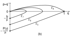
Figure 1. Trajectories corresponding to the equation $q^{\prime\prime}+\gamma q^{\prime}+f(q)=0$. (a) The case $\gamma\in(-c_{0},c_{0})$; (b) the case $\gamma\leqslant-c_{0}$.

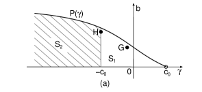
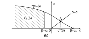
Figure 2. (a) The $\gamma$-$b$ plane about stationary solutions: each point in $S_{1}$ (resp. $S_{2}$) corresponds to a compactly supported solution (resp. a tadpole-like solution); (b) the $c$-$b$ plane about traveling waves, point $A$ corresponds to a rightward traveling semi-wave satisfying both the equation and Stefan boundary condition.

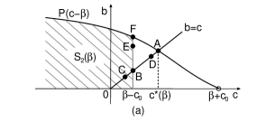
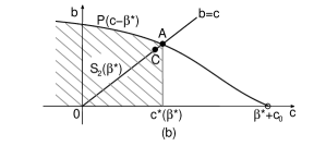
Figure 3. Points $A$ and $F$ correspond to traveling semi-waves, points $B,\ C,\ E$ correspond to tadpole-like traveling waves, point $D$ corresponds to a compactly supported traveling wave, the waves denoted by $A,\ B,\ C,\ D$ satisfy Stefan boundary condition. (a) The case $c_{0}\leqslant\beta<\beta^{*}$; (b) the case $\beta=\beta^{*}$.

(v) Tadpole-like solutions in case $\gamma\leqslant-c_{0}$: $q(\cdot)=V(\cdot-z_{0};b,\gamma)$ for any $z_{0}\in\mathbb{R}$, where for each $b\in(0,P(\gamma))$, $V\in C^{2}((-\infty,0])$ is the unique solution of (3.4) in $(-\infty,0)$ with $V(0;b,\gamma)=0$, $V(-\infty;b,\gamma)=0$ and $b=-\mu V^{\prime}(0;b,\gamma)$ (see $\Gamma_{6}$ and $\Gamma_{7}$ in Figure 1 (b)). Each point $(\gamma,b)$ in the set $S_{2}:=\{(\gamma,b)\mid 0<b<P(\gamma),\;\gamma\leqslant-c_{0}\}$ in Figure 2 (a) corresponds to such a tadpole-like solution $V(z;b,\gamma)$.

We call $V$ a tadpole-like solution since its graph has a big “head” and a boundary on the right side, and an infinite long “tail” on the left side. Similarly, when we construct a traveling wave with the form $V(x-ct;b,\gamma)$, we call it a tadpole-like traveling wave.

(vi) Strictly increasing solutions in $\mathbb{R}$ in case $\gamma\leqslant-c_{0}$: $q(\cdot)=Q(\cdot-z_{0};\gamma)$ for any $z_{0}\in\mathbb{R}$, where $Q\in C^{2}(\mathbb{R})$ is the unique solution of (3.4) in $\mathbb{R}$ with $Q(-\infty;\gamma)=0$, $Q(\infty;\gamma)=1$, $Q(0;\gamma)=1/2$ and $Q^{\prime}(z;\gamma)>0$ in $\mathbb{R}$ (see $\Gamma_{8}$ in Figure 1 (b)).

Each nonnegative stationary solution of ($P$)₁ is a solution of the problem (3.4) with $\gamma=-\beta$. Using the above results we see that, when $\beta\in(0,c_{0})$, a bounded, nonnegative stationary solution of ($P$)₁ is either $0$, or $1$, or a strictly decreasing solutions $U(\cdot-z_{0};-\beta)\ (z_{0}\in\mathbb{R})$ defined on $(-\infty,z_{0}]$, or a compactly supported solution $W(\cdot-z_{0};b,-\beta)\ (z_{0}\in\mathbb{R})$ for some $b\in(0,P(-\beta))=(0,-\mu U^{\prime}(0;-\beta))$, or a strictly increasing solution $U_{l}(\cdot-z_{0};-\beta)\ (z_{0}\in\mathbb{R})$ defined on $[z_{0},\infty)$. When $\beta\geqslant c_{0}$, a bounded, nonnegative stationary solution of ($P$)₁ is either $0$, or $1$, or a strictly decreasing solutions $U(\cdot-z_{0};-\beta)\ (z_{0}\in\mathbb{R})$ defined on $(-\infty,z_{0}]$, or a tadpole-like function $V(\cdot-z_{0};b,-\beta)\ (z_{0}\in\mathbb{R})$ for some $b\in(0,P(-\beta))=(0,-\mu U^{\prime}(0;-\beta))$, or a strictly increasing solution $Q(\cdot-z_{0};-\beta)\ (z_{0}\in\mathbb{R})$ defined in $\mathbb{R}$.

3.3. Traveling waves

If $u(t,x)=q(x-ct)$ is a traveling wave of $u_{t}=u_{xx}-\beta u_{x}+f(u)$, then $(c,q)$ solves (3.4) with $\gamma=c-\beta$, that is,

(3.7) $$q^{\prime\prime}(z)+(c-\beta)q^{\prime}(z)+f(q)=0.$$

In this paper we will use several types of traveling waves which are specified now.

(I) Traveling wave $Q(x-ct;c-\beta)$ for any $c\leqslant\beta-c_{0}$, where $q(z)=Q(z;c-\beta)$ satisfies (3.7) and

(3.8) $$q(-\infty)=0,\ q(\infty)=1,\ q(0)=\frac{1}{2},\ q^{\prime}(z)>0\mbox{ for }z\in\mathbb{R}.$$

The existence of such solutions has been given in the previous subsection.

(II) Rightward traveling semi-wave $U^{*}(x-c^{*}t)$ with $c^{*}\in(0,c_{0}+\beta)$, where $q(z)=U^{*}(z):=U(z;c^{*}-\beta)$ satisfies (3.7) with $c=c^{*}$ and

(3.9) $$q(0)=0,\ q(-\infty)=1,\ -\mu q^{\prime}(0)=c^{*},\ q^{\prime}(z)<0\mbox{ for }z\in(-\infty,0],$$

that is, $(c^{*},U^{*}(z))$ is a solution of (1.5) (cf. point A in Figure 2 (b) and in Figure 3). $U^{*}(x-c^{*}t)$ is called a traveling semi-wave as in [13] since $U^{*}(z)$ is defined only on the half-line $(-\infty,0]$.

Lemma 3.4.

Assume $\beta>0$. Then

• there exists a unique $c^{*}=c^{*}(\beta)\in(0,c_{0}+\beta)$ such that the problem (3.7) and (3.9) with $c=c^{*}$ has a solution, which is unique and denoted by $U^{*}(z)$;

• $0<\frac{\rm d}{{\rm d}\beta}c^{*}(\beta)<1$ for $\beta>0$;

• there exists a unique $\beta^{*}>c_{0}$ such that

  (3.10) $$c^{*}(\beta)-\beta+c_{0}>0\ \ {\rm(}\mbox{resp. }=0,\ <0{\rm)}\ \mbox{ when }\ \beta<\beta^{*}\ \ {\rm(}\mbox{resp. }\beta=\beta^{*},\ \beta>\beta^{*}{\rm)}.$$

Proof.

(i) For any $c<c_{0}+\beta$, the problem (3.4) with $\gamma=c-\beta<c_{0}$ has a unique strictly decreasing solution $q(\cdot)=U(\cdot;c-\beta)$ in $(-\infty,0]$, satisfying $U(0;c-\beta)=0$, $U(-\infty;c-\beta)=1$ and $U^{\prime}(\cdot;c-\beta)<0$ in $(-\infty,0]$. Denote $P(c-\beta):=-\mu U^{\prime}(0;c-\beta)$ as above, then $P(c-\beta)$ is strictly decreasing in $c\in(-\infty,c_{0}+\beta)$,

$$(P(c-\beta)-c)\big{|}_{c=0}=P(-\beta)>0\quad\mbox{and}\quad(P(c-\beta)-c)\big{|}_{c=c_{0}+\beta-0}=-c_{0}-\beta<0$$

(see Figure 2 (b)). Hence the equation $P(c-\beta)=c$ has a unique root $c=c^{*}(\beta)\in(0,c_{0}+\beta)$, that is,

(3.11) $$c^{*}(\beta)=P(c^{*}(\beta)-\beta)=-\mu U^{\prime}(0;c^{*}(\beta)-\beta).$$

(ii) Differentiating $P(c^{*}(\beta)-\beta)=c^{*}(\beta)$ in $\beta$ and using the fact $P^{\prime}(\gamma)<0$ for $\gamma<c_{0}$ we have

$$\frac{{\rm d}c^{*}(\beta)}{{\rm d}\beta}=\frac{-P^{\prime}(c^{*}(\beta)-\beta)}{1-P^{\prime}(c^{*}(\beta)-\beta)}\in(0,1).$$

(iii) Set $\beta^{*}:=P(-c_{0})+c_{0}>c_{0}$. Then $c=\beta^{*}-c_{0}$ is a root of $P(c-\beta^{*})=c$ in $(0,c_{0}+\beta^{*})$. By the definition of $c^{*}(\beta)$ and by its uniqueness we have $\beta^{*}-c_{0}=c^{*}(\beta^{*})$. Moreover, the inequalities in (ii) shows that the function $c^{*}(\beta)-\beta+c_{0}$ is strictly decreasing in $\beta>0$ and so it has a unique zero $\beta^{*}$. This proves (3.10). ∎

(III) Leftward traveling semi-wave $U^{*}_{l}(x-c^{*}_{l}t)$ in case $\beta\in(0,c_{0})$, where $c_{l}^{*}=c^{*}_{l}(\beta)\in(\beta-c_{0},0)$, $q(z)=U^{*}_{l}(z):=U_{l}(z;c^{*}_{l}-\beta)$ satisfies (3.7) with $c=c^{*}_{l}$ and

(3.12) $$q(0)=0,\ q(\infty)=1,\ -\mu q^{\prime}(0)=c^{*}_{l},\ q^{\prime}(z)>0\mbox{ for }z\in[0,\infty).$$

For any given $\beta\in(0,c_{0})$, the existence and uniqueness of such a solution can be proved as in Lemma 3.4 (i).

(IV) Tadpole-like traveling wave $V(x-ct;b,c-\beta)$ in case $\beta>c_{0}$. For any $c\in(0,\beta-c_{0}]$ and any $b\in(0,P(c-\beta))$, $V(x-ct;b,c-\beta)$ is a tadpole-like traveling wave if the function $q(z):=V(z;b,c-\beta)$ satisfies (3.7) and

(3.13) $$q(0)=q(-\infty)=0,\ q(z)>0\mbox{ for }z\in(-\infty,0)\ \mbox{and}\ -\mu q^{\prime}(0)=b$$

(cf. points $B,\ C,\ E$ in Figure 3 (a)). In particular, when $b=c$, the function $V(z;c,c-\beta)$ is a solution of (3.7) and

(3.14) $$q(0)=q(-\infty)=0,\ q(z)>0\mbox{ for }z\in(-\infty,0)\ \mbox{and}\ -\mu q^{\prime}(0)=c$$

(cf. points $B,\ C$ in Figure 3 (a)). On the existence of such solutions we have the following results.

Lemma 3.5.

Let $\beta^{*}$ be the constant given in Lemma 3.4. Assume $c_{0}<\beta<\beta^{*}$. Then

• for any $b\in(0,P(-c_{0}))$, (3.13) and (3.7) with $c=\beta-c_{0}$ has a unique tadpole-like solution $V(z;b,-c_{0})$ (cf. points $B,\ E$ in Figure 3 (a)). Moreover, there exists $z_{b}<0$ such that

  (3.15) $$V(\cdot+z_{b};b,-c_{0})\to Q(\cdot)\mbox{ locally uniformly in }\mathbb{R},\quad\mbox{as }b\to P(-c_{0});$$

• $q(z)=V^{*}(z):=V(z;\beta-c_{0},-c_{0})$ is the unique tadpole-like solution of (3.7) and (3.14) with $c=\beta-c_{0}$, that is, the unique solution of (2.7);

• for any $\delta\in(0,\beta-c_{0})$, $q(z)=V_{\delta}(z):=V(z;\beta-c_{0}-\delta,-c_{0}-\delta)$ is a tadpole-like solution of (3.7) and (3.14) with $c=\beta-c_{0}-\delta$. Moreover, $V_{\delta}(z)\to V^{*}(z)$ locally uniformly in $(-\infty,0]$ as $\delta\to 0$ (cf. point $C$ in Figure 3 (a)).

Proof.

(i) Since $c_{0}<\beta<\beta^{*}$, we have $0<\beta-c_{0}<c^{*}$ by Lemma 3.4. On the $c$-$b$ plane (see Figure 3 (a)), any point $E(\beta-c_{0},b)$ with $b\in(0,P(-c_{0}))$ corresponds to a tadpole-like solution $V(z;b,-c_{0})$ of (3.13) and (3.7) with $c=\beta-c_{0}$ (cf. trajectories $\Gamma_{6}$ or $\Gamma_{7}$ in Figure 1 (b). Note that such a solution does not necessarily satisfy Stefan condition since $b$ may be not equal to $c$). As $b\to P(\beta-c_{0})$ (i.e., point $E$ moves up to $F$ in Figure 3 (a)), the trajectory of $V(z;b,-c_{0})$ approaches the union of the trajectories of $Q$ and $U^{*}$ (i.e., $\Gamma_{6}\to\Gamma_{5}\cup\Gamma_{8}$). Denote $z_{b}:=\min\{z<0\mid V(z;b,-c_{0})=\frac{1}{2}\}$. Then the trajectory of $V(\cdot+z_{b};b,-c_{0})$ approaches that of $Q(\cdot)$ (since $Q(0)=\frac{1}{2}$), and so we obtain (3.15) by continuity.

(ii) On the $c$-$b$ plane, the line $\{b=c\}$ passes through the domain $S_{2}(\beta):=\{(c,b)\mid 0<b<P(c-\beta),0<c<\beta-c_{0}\}$ and leaves it at a point $B(\beta-c_{0},\beta-c_{0})$. This point corresponds to the desired tadpole-like solution $V^{*}(z):=V(z;\beta-c_{0},-c_{0})$.

(iii) For any small $\delta>0$, we consider the point $C(\beta-c_{0}-\delta,\beta-c_{0}-\delta)$ on the $c$-$b$ plane. Since $C\in S_{2}(\beta)\cap\{b=c\}$, it corresponds to a tadpole-like solution $V_{\delta}(z):=V(z;\beta-c_{0}-\delta,-c_{0}-\delta)$ of (3.7) and (3.14) with $c=\beta-c_{0}-\delta$. In particular, $V_{\delta}(z)$ satisfies the following initial value problem

$$\left\{\begin{array}[]{l}q^{\prime\prime}(z)-(c_{0}+\delta)q^{\prime}(z)+f(q)=0,\ \ z<0,\\ q(0)=0,\ \ -\mu q^{\prime}(0)=\beta-c_{0}-\delta.\end{array}\right.$$

Since $V^{*}$ satisfies this problem with $\delta=0$ and since $V_{\delta}$ depends on $\delta$ continuously, we have $V_{\delta}(\cdot)\to V^{*}(\cdot)$ as $\delta\to 0$, uniformly in $[-M,0]$ for any $M>0$. This proves the lemma. ∎

In a similar way, one can prove the following lemma (cf. Figure 3 (b)).

Lemma 3.6.

Assume $\beta=\beta^{*}$. Then for any small $\delta>0$, $q(z)=V^{*}_{\delta}(z):=V(z;\beta^{*}-c_{0}-\delta,-c_{0}-\delta)$ is the unique tadpole-like solution of (3.7) and (3.14) with $\beta=\beta^{*}$, $c=\beta^{*}-c_{0}-\delta$. Moreover, $V^{*}_{\delta}(\cdot)\to U^{*}(\cdot)$ locally uniformly in $(-\infty,0]$ as $\delta\to 0$, where $U^{*}(z)$ is the unique solution of (3.7) and (3.9) with $\beta=\beta^{*}$, $c^{*}=c^{*}(\beta^{*})=\beta^{*}-c_{0}$.

(V) Compactly supported traveling wave $W(x-ct;c,c-\beta)$ in case $\beta\in[c_{0},\beta^{*})$, where for any $c\in(\beta-c_{0},c^{*}(\beta))$, $q(z)=W(z;c,c-\beta)$ satisfies (3.7) and

(3.16) $$q(0)=q(-L(c,c-\beta))=0,\quad q(z)>0\mbox{ in }(-L(c,c-\beta),0)\quad\mbox{and}\quad-\mu q^{\prime}(0)=c.$$

Lemma 3.7.

Assume $c_{0}\leqslant\beta<\beta^{*}$. For any $\delta\in(0,c^{*}(\beta)-\beta+c_{0})$, $q(z)=W_{\delta}(z):=W(z;\beta-c_{0}+\delta,-c_{0}+\delta)$ is the unique solution of the problem (3.7) and (3.16) with $c=\beta-c_{0}+\delta$. Moreover, $L_{\delta}\to\infty$ and $D_{\delta}\to 1$ as $\delta\to c^{*}(\beta)-\beta+c_{0}$, where $L_{\delta}:=L(\beta-c_{0}+\delta,-c_{0}+\delta)$ denotes the width of the support of $W_{\delta}(\cdot)$, and $D_{\delta}$ denotes its height.

Proof.

We only prove the case $\beta\in(c_{0},\beta^{*})$, the proof for the case $\beta=c_{0}$ is similar.

When $c_{0}<\beta<\beta^{*}$, we have $c^{*}(\beta)-\beta+c_{0}>0$ by Lemma 3.4. On the $c$-$b$ plane (see Figure 3 (a)), the line $b=c$ leaves the domain $S_{2}(\beta)$ and enters $S_{1}(\beta):=\{(c,b)\mid 0<b<P(c-\beta),\ \beta-c_{0}<c<\beta+c_{0}\}$ at a point $B(\beta-c_{0},\beta-c_{0})$, then it passes through $S_{1}(\beta)$ and leaves it finally at $A(c^{*}(\beta),c^{*}(\beta))$. For any $\delta\in(0,c^{*}(\beta)-\beta+c_{0})$, the point $(c,b)=(\beta-c_{0}+\delta,\beta-c_{0}+\delta)$ is on the line segment $AB$ (cf. point $D$ in Figure 3 (a)), it corresponds to a trajectory like $\Gamma_{2}$ on the $q$-$p$ phase plane, and so it defines a compactly supported function $W_{\delta}(z):=W(z;\beta-c_{0}+\delta,-c_{0}+\delta)$. As $\delta\to c^{*}(\beta)-\beta+c_{0}$, the point $(\beta-c_{0}+\delta,\beta-c_{0}+\delta)$ approaches point $A$ in Figure 3 (a), this implies that its corresponding trajectory approaches the union of the trajectories of $U^{*}(\cdot)$ and $U_{l}(\cdot;c^{*}(\beta)-\beta)$ (i.e., $\Gamma_{2}\to\Gamma_{1}\cup\Gamma_{4}$ in Figure 1 (a)). Therefore, the corresponding function $W_{\delta}$ satisfies $\max\limits_{-L_{\delta}\leqslant z\leqslant 0}W_{\delta}(z)=D_{\delta}\to 1$, and the width $L_{\delta}$ of its support tends to $\infty$ as $\delta\to c^{*}(\beta)-\beta+c_{0}$. ∎

3.4. Zero number arguments

In what follows, we use $\mathcal{Z}_{I}[w(\cdot)]$ to denote the number of zeros of a continuous function $w(\cdot)$ defined in $I\subset\mathbb{R}$. The following lemma is an easy consequence of the proofs of Theorems C and D in Angenent [1].

Lemma 3.8.

Let $u:[0,T]\times[0,1]\to\mathbb{R}$ be a bounded classical solution of

(3.17) $$u_{t}=a(t,x)u_{xx}+b(t,x)u_{x}+c(t,x)u$$

with boundary conditions

$$u(t,0)=l_{0}(t),\;u(t,1)=l_{1}(t),$$

where $l_{0},l_{1}\in C^{1}([0,T])$, and each function is either identically zero or never zero for $t\in[0,T]$. In the special case where $l_{0}(t),\ l_{1}(t)\equiv 0$ we assume further that $u(t,\cdot)\not\equiv 0$ for each $t\in[0,T]$. Suppose also that

$$a,1/a,a_{t},a_{x},a_{xx},b,b_{t},b_{x},c\in L^{\infty},\mbox{ and }u(0,\cdot)\not\equiv 0\mbox{ when $l_{0}=l_{1}\equiv 0$}.$$

Then for each $t\in(0,T]$, $\mathcal{Z}_{[0,1]}[u(t,\cdot)]<\infty$. Moreover, $\mathcal{Z}_{[0,1]}[u(t,\cdot)]$ is nonincreasing in $t$ for $t\in(0,T]$, and if for some $t_{0}\in(0,T]$ the function $u(t_{0},\cdot)$ has a degenerate zero $x_{0}\in[0,1]$, then $\mathcal{Z}_{[0,1]}[u(t_{1},\cdot)]>\mathcal{Z}_{[0,1]}[u(t_{2},\cdot)]$ for all $t_{1},t_{2}\in(0,T]$ satisfying $t_{1}<t_{0}<t_{2}$.

For convenience of applications in this paper we give a variant of Lemma 3.8.

Lemma 3.9.

Let $\xi_{1}(t)<\xi_{2}(t)$ be two continuous functions for $t\in(t_{0},t_{1})$. If $u(t,x)$ is a continuous function for $t\in(t_{0},t_{1})$ and $x\in J(t):=[\xi_{1}(t),\xi_{2}(t)]$, and satisfies (3.17) in the classical sense for such $(t,x)$, with

$$u(t,\xi_{1}(t))\not=0,\;u(t,\xi_{2}(t))\not=0\mbox{ for }t\in(t_{0},t_{1}),$$

then for each $t\in(t_{0},t_{1})$, $\mathcal{Z}_{J(t)}[u(t,\cdot)]<\infty$. Moreover $\mathcal{Z}_{J(t)}[u(t,\cdot)]$ is nonincreasing in $t$ for $t\in(t_{0},t_{1})$, and if for some $s\in(t_{0},t_{1})$ the function $u(s,\cdot)$ has a degenerate zero $x_{0}\in J(s)$, then $\mathcal{Z}_{J(s_{1})}[u(s_{1},\cdot)]>\mathcal{Z}_{J(s_{2})}[u(s_{2},\cdot)]$ for all $s_{1},s_{2}$ satisfying $t_{0}<s_{1}<s<s_{2}<t_{1}$.

Proof.

For any given $t^{*}\in(t_{0},t_{1})$, we can find $\epsilon>0$ and $\delta>0$ small such that $u(t,x)\not=0$ for $t\in T_{t^{*}}:=[t^{*}-\delta,t^{*}+\delta]\subset(t_{0},t_{1})$ and $x\in[\xi_{1}(t),\xi_{1}(t^{*})+\epsilon]\cup[\xi_{2}(t^{*})-\epsilon,\xi_{2}(t)]$. Hence we may apply Lemma 3.8 with $[0,T]\times[0,1]$ replaced by $T_{t^{*}}\times[\xi_{1}(t^{*})+\epsilon,\xi_{2}(t^{*})-\epsilon]$ to see that the conclusions for $\mathcal{Z}_{J(t)}[u(t,\cdot)]$ hold for $t\in T_{t^{*}}$. Since any compact subinterval of $(t_{0},t_{1})$ can be covered by finitely many such $T_{t^{*}}$, we see that $\mathcal{Z}_{J(t)}[u(t,\cdot)]$ has the required properties over any compact subinterval of $(t_{0},t_{1})$. It follows that $\mathcal{Z}_{J(t)}[u(t,\cdot)]$ has the required properties for $t\in(t_{0},t_{1})$. ∎

In our approach we will compare the solution $u$ of ($P$) with traveling semi-wave $U^{*}$ or tadpole-like traveling wave $V^{*}$ or compactly supported traveling wave $W_{\delta}$ by studying the number of their intersection points. Now we give some preliminary results.

We use $\Psi(x-ct-C)$ (for some $c>0$ and some $C\in\mathbb{R}$) to represent one of the traveling waves $U^{*}(x-c^{*}t-C)$, $V^{*}(x-(\beta-c_{0})t-C)$ and $W_{\delta}(x-(\beta-c_{0}+\delta)t-C)$. Denote the support of $\Psi(x-ct-C)$ by $[k_{1}(t),k_{2}(t)]$, where $k_{2}(t)=ct+C$, $k_{1}(t)=-\infty$ in case $\Psi=U^{*}$ or $\Psi=V^{*}$, and $k_{1}(t)=k_{2}(t)-L_{\delta}$ in case $\Psi=W_{\delta}$. Denote

$$r(t):=\min\{h(t),k_{2}(t)\},\quad R(t):=\max\{h(t),k_{2}(t)\},\quad l(t):=\max\{g(t),k_{1}(t)\}$$

and

$$\eta(t,x):=u(t,x)-\Psi(x-ct-C),\quad x\in J(t):=[l(t),r(t)],\ t\in(t_{1},t_{2})$$

(here we only consider the case where $J(t)\neq\emptyset$ for each $t\in(t_{1},t_{2})$, otherwise, $u$ and $\Psi$ has no common domain and so there is no need to compare them). We notice that $\eta$ satisfies

$$\eta_{t}=\eta_{xx}-\beta\eta_{x}+c(t,x)\eta\quad\mbox{for }x\in(l(t),r(t)),\ t\in(t_{1},t_{2})$$

with $c(t,x):=[f(u(t,x))-f(\Psi(x-ct-C))]/\eta(t,x)$ when $\eta(t,x)\neq 0$, and $c(t,x)=0$ otherwise. Using Lemmas 3.8 and 3.9 one can obtain the following result on the number of zeros of $\eta(t,\cdot)$.

Lemma 3.10.

For any given $C\in\mathbb{R}$, let $r(t),\ R(t),\ l(t)$ and $\eta$ be defined as above. Then

• $\mathcal{Z}_{J(t)}[\eta(t,\cdot)]$ is finite and nonincreasing in $t\in(t_{1},t_{2})$;

• if $t_{0}\in(t_{1},t_{2})$ such that $r(t_{0})=R(t_{0})$, or $\eta(t_{0},\cdot)$ has a degenerate zero in the interior of $J(t_{0})$, then $\mathcal{Z}_{J(\tau_{1})}[\eta(\tau_{1},\cdot)]>\mathcal{Z}_{J(\tau_{2})}[\eta(\tau_{2},\cdot)]$ for any $t_{1}<\tau_{1}<t_{0}<\tau_{2}<t_{2}$.

Sketch of the proof. The proof is essentially identical to that of Lemma 2.3 in [14]. We give a sketch here for the readers’ convenience.

Note that when $h(t)=k_{2}(t)=r(t)=R(t)$, $x=r(t)$ becomes a degenerate zero of $\eta$ on the boundary since both $u$ and $\Psi$ satisfy Stefan condition on their right boundaries. We claim that $h(t)\equiv k_{2}(t)$ in an interval $(t_{3},t_{4})\subset(t_{1},t_{2})$ is impossible. For, otherwise, we can consider $\zeta=\eta e^{-\frac{\beta}{2}x}$ instead of $\eta$, which satisfies an equation without advection and so can be extended outside $r(t)$ as an odd function with respect to $x=r(t)$. For this extended function $x=r(t)$ is an interior degenerate zero in time interval $(t_{3},t_{4})$, this contradicts Lemma 3.8. On the other hand, $g(t)=k_{1}(t)$ at most once, and only possible in case $\Psi=W_{\delta}$. Therefore, the set of the times when $r(t)=R(t)$ or $g(t)=k_{1}(t)$ is a nowhere dense set, and for other times we have $\mathcal{Z}_{J(t)}[\eta(t,\cdot)]<\infty$ by Lemma 3.8.

Assume $r(t_{0})=R(t_{0})$ and $r(t)<R(t)$ for $t\in[t_{0}-\epsilon,t_{0})$. Assume further that $\eta(t,\cdot)$ has nondegenerate zeros $\{z_{i}(t)\}_{i=1}^{m}$ with

$$l(t)<z_{1}(t)<z_{2}(t)<\cdots<z_{m}(t)<r(t),\quad t\in[t_{0}-\epsilon,t_{0}).$$

Then by [19, Theorem 2] one can prove that $\lim\limits_{t\to t_{0}}z_{i}(t)$ exist (denoted by $\bar{z}_{i}$) and $\{\bar{z}_{i}\}_{i=1}^{m}$ are the only zeros of $\eta(t_{0},\cdot)$. Moreover, by the maximum principle we have $\bar{z}_{m}=r(t_{0})$, that is, the largest zero $z_{m}(t)$ tends to the right boundary. Then using the maximum principle again in the domain $\{(t,x)\mid t_{0}<t<t_{0}+\epsilon_{1},r(t)-\epsilon_{1}<z<r(t)\}$ for some small $\epsilon_{1}$, we can show that the boundary zero $r(t_{0})$ disappear immediately after time $t_{0}$. In summary,

$$\mathcal{Z}_{J(\tau_{1})}[\eta(\tau_{1},\cdot)]=m\geqslant\mathcal{Z}_{J(t_{0})}[\eta(t_{0},\cdot)]>\mathcal{Z}_{J(\tau_{2})}[\eta(\tau_{2},\cdot)]$$

for $t_{0}-\epsilon<\tau_{1}<t_{0}<\tau_{2}<t_{0}+\epsilon_{1}$. $\Box$

As can be expected, the presence of the advection makes the maximum points prefer to move rightward. Indeed we can show that the local maximum points concentrate near the right boundary under certain conditions.

Using zero number properties Lemma 3.9 to $u_{x}$, we see that $u_{x}(t,\cdot)$ has only nondegenerate zeros for all large $t$. Hence, $u(t,\cdot)$ has fixed number of (nondegenerate) local maximum points for large $t$.

Lemma 3.11.

Assume, for some $T\geqslant 0$, $u(t,\cdot)$ has exactly $N$ ($N$ is a positive integer) local maximum points $\{\xi_{i}(t)\}_{i=1}^{N}$ for all $t\geqslant T$, with

$$g(t)<\xi_{1}(t)<\xi_{2}(t)<\cdots<\xi_{N}(t)<h(t).$$

If $N\geqslant 2$, then

(3.18) $$\xi_{1}(t)\geqslant\beta\cdot(t-T)+C\quad\mbox{for }T\leqslant t<T_{\infty},$$

for some $C\in\mathbb{R}$, where

(3.19) $$T_{\infty}=\left\{\begin{array}[]{ll}\inf\mathcal{T},&\mbox{ if }\mathcal{T}:=\{t\geqslant T\mid\beta\cdot(t-T)+C=h(t)\}\neq\emptyset,\\ \infty,&\mbox{ if }\mathcal{T}=\emptyset.\end{array}\right.$$

Proof.

Choose $C=\frac{1}{2}[g(T)+\xi_{1}(T)]$ and define $\rho(t):=\beta(t-T)+C$, then $\rho(T)=C<\xi_{1}(T)$. Hence $T_{1}:=\inf\{s\geqslant T\mid\rho(s)=\xi_{1}(s)\}>T$.

If $T_{1}=T_{\infty}$, then (3.18) holds. Now we assume $T<T_{1}<T_{\infty}$. By the definitions of $\xi_{1}(t)$ and $T_{1}$ we have

(3.20) $$u_{x}(t,x)>0\quad\mbox{for }x\in[g(t),\rho(t)],\ T\leqslant t<T_{1},$$

and

(3.21) $$u_{x}(T_{1},\rho(T_{1}))=u_{x}(T_{1},\xi_{1}(T_{1}))=0.$$

Define

$$\zeta(t,x):=u(t,x)-u(t,2\rho(t)-x)\quad\mbox{for }x\in[l(t),\rho(t)],\ t\geqslant T,$$

with $l(t):=\max\{g(t),2\rho(t)-\xi_{N}(t)\}$. A direct calculation shows that

$$\zeta_{t}=\zeta_{xx}-\beta\zeta_{x}+c\zeta\quad\mbox{for }x\in[l(t),\rho(t)],\ t\in[T,T_{1}),$$

where $c$ is a bounded function. Since

$$\left\{\begin{array}[]{ll}\zeta(T,x)<0&\mbox{ for }x\in[l(T),\rho(T)],\\ \zeta(t,\rho(t))=0&\mbox{ for }t\in[T,T_{1}],\\ \zeta(t,l(t))<0&\mbox{ for }t\in[T,T_{1}].\end{array}\right.$$

The last inequality follows from the following analysis. By the monotonicity of $u_{x}$ and the fact that $\xi_{N}(t)$ is the rightmost local maximum point, we see that, if $\zeta(t_{1},l(t_{1}))=0$ for some $t_{1}\in(T,T_{1}]$ (denote $t_{1}$ the first of such times), then $\zeta(t_{1},l(t_{1})+\varepsilon)>0$ for some small $\varepsilon>0$. This, however, is impossible since $\zeta(t_{1},x)<0$ for all $x\in(l(t_{1}),\rho(t_{1}))$ by the maximum principle and by the fact that $\zeta(t,l(t))<0$ for $t\in[T,t_{1})$.

Now we use the Hopf lemma for $\zeta$ in the domain $\{(t,x)\mid l(t)\leqslant x\leqslant\rho(t),\ T\leqslant t\leqslant T_{1}\}$ to derive

$$\zeta(T_{1},\rho(T_{1}))=0\quad\mbox{and}\quad\zeta_{x}(T_{1},\rho(T_{1}))>0.$$

The latter, however, contradicts (3.21). This proves $T_{1}=T_{\infty}$. ∎

3.5. Upper bound estimate

In order to study the convergence of $u$ we give some precise upper bound estimates for the solutions. In this paper we always write

(3.22) $$A:=2\max\big{\{}1,\|u_{0}\|_{L^{\infty}([-h_{0},h_{0}])}\big{\}}.$$

1. Bound of $u$ near the free boundary $x=h(t)$. For any $\delta\in(0,-f^{\prime}(1))$, set

$$\bar{g}(t):=g(t),\quad\bar{h}(t):=c^{*}t-Me^{-\delta t}+H\ \mbox{ for some }M,\ H>0,$$

and

$$\bar{u}(t,x):=(1+Ae^{-\delta t})U^{*}(x-\bar{h}(t))\ \mbox{ for }x\leqslant\bar{h}(t),\ t>0,$$

where $U^{*}$ is the rightward traveling semi-wave (the solution of (1.5)). A direct calculation as in the proof of [17, Lemma 3.2] shows that $(\bar{u},\bar{g},\bar{h})$ is an upper solution of ($P$) provided $M,H>0$ are large. Hence we have

(3.23) $$u(t,x)\leqslant\bar{u}(t,x)\mbox{ for }x\in[g(t),h(t)]\mbox{ and }t>0,\quad h(t)\leqslant\bar{h}(t)\mbox{ for }t>0.$$

2. Bound of $u$ in case $\beta\geqslant c_{0}$. We define a function $f_{A}(s)\in C^{2}([0,\infty),\mathbb{R})$ such that

(3.24) $$f_{A}(s)\left\{\begin{array}[]{ll}=f^{\prime}(0)s,&0\leqslant s\leqslant 1,\\ >0,&1<s<A,\\ <0,&s>A,\end{array}\right.\quad f^{\prime}_{A}(A)<0,\quad f(s)\leqslant f_{A}(s)\leqslant f^{\prime}(0)s\ \mbox{for}\ s\geqslant 0.$$

Denote by $Q_{A}(z)$ the unique solution of (1.4) with $c=c_{0}$, with $f$ replaced by $f_{A}$ and $q(+\infty)=1$ replaced by $q(+\infty)=A$. Then by the comparison principle we have

(3.25) $$u(t,x)\leqslant Q_{A}(x-(\beta-c_{0})t+x_{0})\quad\mbox{for }x\in[g(t),h(t)],\;t>0,$$

provided $x_{0}>0$ is large enough.

Using $f_{A}$ we consider the Cauchy problem:

$$\left\{\begin{array}[]{l}(u_{1})_{t}=(u_{1})_{xx}-\beta(u_{1})_{x}+f_{A}(u_{1}),\quad x\in\mathbb{R},\;t>0,\\ u_{1}(0,x)=\tilde{u}_{0}(x):=\left\{\begin{array}[]{ll}u_{0}(x),&x\in[-h_{0},h_{0}],\\ 0,&|x|>h_{0}.\end{array}\right.\end{array}\right.$$

Since $f_{A}\geqslant f$, by the comparison principle we have

(3.26) $$u(t,x)\leqslant u_{1}(t,x),\quad x\in[g(t),h(t)],\;t>0.$$

Set $y:=x-\beta t$ and $u_{2}(t,y):=u_{1}(t,x)=u_{1}(t,y+\beta t)$. Then $u_{2}$ is a solution of

$$\left\{\begin{array}[]{l}(u_{2})_{t}=(u_{2})_{yy}+f_{A}(u_{2}),\quad y\in\mathbb{R},\;t>0,\\ u_{2}(0,y)=\tilde{u}_{0}(y)\in[0,A],\quad y\in\mathbb{R}.\end{array}\right.$$

Set $\tilde{u}(t,y):=\frac{1}{A}u_{2}(t,-y)$, then $\tilde{u}(t,y)$ is the solution of

$$\left\{\begin{array}[]{l}\tilde{u}_{t}=\tilde{u}_{yy}+\frac{1}{A}f_{A}\big{(}A\tilde{u}\big{)},\quad y\in\mathbb{R},\;t>0,\\ \tilde{u}(0,y)=\frac{1}{A}\tilde{u}_{0}(-y)\in[0,1],\quad y\in\mathbb{R}.\end{array}\right.$$

By (3.26) and by the definitions of $u_{2}$ and $\tilde{u}$ we have

(3.27) $$u(t,x)\leqslant A\tilde{u}(t,\beta t-x),\quad x\in[g(t),h(t)],\;t>0.$$

On the other hand, by Proposition 2.3 in [25] and its proof, there exist $C_{1},C_{2},t_{0}$ depending on $u_{0}$ such that

$$\tilde{u}\Big{(}t,c_{0}t-\frac{3}{c_{0}}\ln\big{(}1+\frac{t}{t_{0}}\big{)}+y\Big{)}\leqslant C_{1}Z(t,y),\quad y\geqslant h_{0},\;t>0,$$

where

(3.28) $$Z(t,y):=\frac{1}{\sqrt{t_{0}}}ye^{-\frac{c_{0}}{2}y}\big{[}C_{2}e^{\frac{-y^{2}}{4(t+t_{0})}}+h(t,y)\big{]},\quad y\in\mathbb{R},t>0,$$

with $h(t,y)$ satisfying

$$\limsup\limits_{t\to\infty}\sup\limits_{0\leqslant y\leqslant\sqrt{t+1}}|h(t,y)|\leqslant\frac{C_{2}}{2}.$$

In particular, there exists $C_{3}>0$ such that

$$\tilde{u}\Big{(}t,c_{0}t-\frac{3}{c_{0}}\ln\big{(}1+\frac{t}{t_{0}}\big{)}+y\Big{)}\leqslant C_{3}e^{-\frac{5c_{0}}{12}y},\quad y\in[0,\sqrt{t+1}].$$

Combining with (3.27) we have

(3.29) $$u(t,x)\leqslant C_{4}e^{-\frac{5c_{0}}{12}(Y(t)-x)}\quad\mbox{for }Y(t)-\sqrt{t+1}\leqslant x\leqslant\min\big{\{}Y(t),h(t)\big{\}},\;t\gg 1,$$

where $C_{4}>0$ is a constant and

(3.30) $$Y(t):=(\beta-c_{0})t+\frac{3}{c_{0}}\ln\big{(}1+\frac{t}{t_{0}}\big{)},\quad t>0.$$

Corollary 3.12.

(i) Assume $\beta=c_{0}$. Then there exists $C$ depending on $u_{0},c_{0},h_{0}$ such that

$$u(t,-h_{0})\leqslant Ct^{-\frac{5}{4}}\quad\mbox{for }t>0\mbox{ large};$$

(ii) Assume $\beta\in(c_{0},\beta^{*}]$ and $h(t)=(\beta-c_{0})t+O(1)$. Then there exists $C$ depending on $u_{0},c_{0},h_{0}$ such that

$$u(t,x)\leqslant Ct^{-\frac{5}{4}}\quad\mbox{for }x\in\Big{[}h(t)-\frac{\pi}{2},h(t)\Big{]}\mbox{ and }t>0\mbox{ large}.$$

Proof.

We only prove (ii) since (i) can be proved similarly. In Case (ii),

$$Y(t)=(\beta-c_{0})t+\frac{3}{c_{0}}\ln\big{(}1+\frac{t}{t_{0}}\big{)},$$

and so, for any $x\in[h(t)-\frac{\pi}{2},h(t)]$, we have

$$Y(t)-x=\frac{3}{c_{0}}\ln\big{(}1+\frac{t}{t_{0}}\big{)}+O(1)\in[0,\sqrt{t+1}],\quad\mbox{when }t\gg 1.$$

Using (3.29) we have

(3.31) $$u(t,x)\leqslant Ct^{-\frac{5}{4}}\quad\mbox{when }t\gg 1,$$

where $C>0$ are some constants depending on $u_{0},c_{0},h_{0}$. ∎

Remark 3.13.

For any given $m\in(0,1)$, denote

$$\chi(t):=\min\{x\in[g(t),h(t)]\mid u(t,x)=m\}\mbox{ and }\widetilde{\chi}(t):=\min\{y\in\mathbb{R}\mid\tilde{u}(t,y)=m/A\}.$$

Then by [25, Theorem 1.1] we have

$$c_{0}t-\frac{3}{c_{0}}\ln t-C\leqslant\widetilde{\chi}(t)\leqslant c_{0}t-\frac{3}{c_{0}}\ln t+C,\quad t\gg 1,$$

for some $C>0$. Hence by (3.27) we have

(3.32) $$\chi(t)\geqslant\beta t-\widetilde{\chi}(t)\geqslant(\beta-c_{0})t+\frac{3}{c_{0}}\ln t-C,\quad t\gg 1.$$

4. Influence of $\beta$ on the long time behavior of solutions

In this section we consider the influence of $\beta$ on the long time behavior of the solutions. In subsection 1 we give a locally uniformly convergence result. In subsection 2 we consider the small advection $\beta\in(0,c_{0})$ and prove Theorem 2.1. In subsection 3 we first prove the boundedness of $g_{\infty}$ for $\beta\geqslant c_{0}$, the boundedness of $h_{\infty}$ for $\beta\geqslant\beta^{*}$, and then prove Theorem 2.4 for large advection $\beta\geqslant\beta^{*}$. In subsection 4, we consider ($P$) with medium-sized advection $\beta\in[c_{0},\beta^{*})$ and prove Theorems 2.2 and 2.3. The argument for the case $\beta\in[c_{0},\beta^{*})$ are longer and much more complicated than the cases with small or large advection.

4.1. Convergence result

First we give a locally uniformly convergence result for $\beta\geqslant c_{0}$.

Lemma 4.1.

Assume $\beta\geqslant c_{0}$. Then $u(t,\cdot)$ converges as $t\to\infty$ to $0$ locally uniformly in $I_{\infty}$.

Proof.

When $\beta>c_{0}$, the conclusion follows easily from (3.25) since the upper solution $Q_{A}(x-(\beta-c_{0})t+x_{0})$ is a rightward traveling wave with positive speed $\beta-c_{0}$ and $Q_{A}(z)\to 0$ as $z\to-\infty$.

Assume $\beta=c_{0}$. Then for any $[a,b]\subset I_{\infty}$, when $t$ is sufficiently large we have

$$\frac{3}{c_{0}}\ln\big{(}1+\frac{t}{t_{0}}\big{)}-\sqrt{t+1}<x<\frac{3}{c_{0}}\ln\big{(}1+\frac{t}{t_{0}}\big{)}\quad\mbox{ for any }x\in[a,b],$$

and so by (3.29), for any $x\in[a,b]$,

$$u(t,x)\leqslant C_{4}e^{-\frac{5c_{0}}{12}\big{[}\frac{3}{c_{0}}\ln\big{(}1+\frac{t}{t_{0}}\big{)}-b\big{]}}\to 0,\quad\mbox{as }t\to\infty.$$

This proved the lemma. ∎

Theorem 4.2.

Let $(u,g,h)$ be a time-global solution of ($P$). Then as $t\to\infty$, $u(t,\cdot)$ converges to $0$ or to $1$ locally uniformly in $I_{\infty}$ when $\beta\in(0,c_{0})$; $u(t,\cdot)$ converges to $0$ locally uniformly in $I_{\infty}$ when $\beta\geqslant c_{0}$.

Moreover, $\lim_{t\to\infty}\|u(t,\cdot)\|_{L^{\infty}([g(t),h(t)])}=0$ if $I_{\infty}$ is a bounded interval.

Proof.

Using a similar argument as proving [15, Theorem 1.1], [13, Theorem 1.1], [32, Theorem 1.1], one can show that $u(t,\cdot)$ converges, as $t\to\infty$, to a stationary solution, that is, a solution $v$ of $v_{xx}-\beta v_{x}+f(v)=0$, locally uniformly in $x\in I_{\infty}$. Moreover, one can show by Hopf lemma that $v=0$ when $g_{\infty}>-\infty$ or $h_{\infty}<\infty$. In other word, the limit $v$ can not be a non-trivial solution with endpoint. Therefore, when $\beta\in(0,c_{0})$, the only possible choice for the $\omega$-limit of $u$ in the topology of $L^{\infty}_{\rm loc}(I_{\infty})$ is $0$ or $1$; when $\beta\geqslant c_{0}$, the conclusion follows from Lemma 4.1. Finally, when $I_{\infty}$ is bounded, the uniform convergence for $u$ is also proved in the same way as that in [13, 32]. ∎

4.2. Problem with small advection: $0<\beta<c_{0}$

In a similar way as proving [23, Lemma 2.2] and [13, Theorem 3.2, Corollary 4.5] one can show the following conditions for spreading and for vanishing.

Lemma 4.3.

Assume $\beta\in(0,c_{0})$. Let $(u,g,h)$ be a solution of ($P$).

(i) If $h_{0}<H^{*}:=\frac{\pi}{\sqrt{{c^{2}_{0}}-\beta^{2}}}$ and if $\|u_{0}\|_{L^{\infty}([-h_{0},h_{0}])}$ is sufficiently small, then vanishing happens;

(ii) if $h_{0}\geqslant H^{*}$, then spreading happens.

This lemma implies that, when $\beta\in(0,c_{0})$, $2H^{*}$ is a critical width of the interval $I(t)$. Spreading happens if and only if $|I_{\infty}|>2H^{*}$. This extends the results in [12, 13] for $\beta=0$, where it was shown that the critical width $2H^{*}=\frac{2\pi}{c_{0}}=\frac{\pi}{\sqrt{f^{\prime}(0)}}$.

Proof of Theorem 2.1: By Lemma 4.3 (ii) we see that spreading happens if $|I_{\infty}|>2H^{*}$. By the definition of spreading, this implies that $I_{\infty}=\mathbb{R}$. Hence both the case $g_{\infty}>-\infty$, $h_{\infty}=\infty$ and the case $g_{\infty}=-\infty$, $h_{\infty}<\infty$ are impossible. $I_{\infty}$ is either a bounded interval with width $|I_{\infty}|\leqslant 2H^{*}$ or the whole line $\mathbb{R}$. Using Theorem 4.2 and Lemma 4.3 again, we can get the spreading-vanishing dichotomy result for the long-time behavior of the solutions of ($P$). Then the sharp threshold of the initial data $\sigma\phi$ can be proved in a similar way as in [13, Theorem 5.2]. $\Box$

4.3. Boundedness of $g_{\infty}$ and $h_{\infty}$, the proof of Theorem 2.4

Whether $g_{\infty}$ and $h_{\infty}$ are bounded or not is also a part of the conclusions in the long time behavior of $(u,g,h)$. In this subsection we show that $g_{\infty}>-\infty$ if $\beta\geqslant c_{0}$, and $h_{\infty}<\infty$ if $\beta\geqslant\beta^{*}$.

We will prove these conclusions by using Corollary 3.12. For this purpose we need the monotonicity of $u_{x}$. When $\beta=0$, Du and Lou [13] proved the monotonicity of $u_{x}$ in $[h_{0},h(t)]$ and in $[g(t),-h_{0}]$. When $\beta>0$ we find that this is true only on the left side: $x\in[g(t),-h_{0}]$.

Lemma 4.4.

Assume $(u,g,h)$ is a solution of ($P$). Then

(4.1) $$g(t)+h(t)>-2h_{0}\quad\mbox{for all }t>0,$$

(4.2) $$u_{x}(t,x)>0\quad\mbox{for all }x\in[g(t),-h_{0}],\ t>0.$$

Proof.

It is easily seen by the continuity that, when $t>0$ is sufficiently small, $g(t)+h(t)>-2h_{0}$ and $u_{x}(t,x)>0$ for $g(t)\leqslant x\leqslant-h_{0}$. Define

$$T_{1}:=\sup\big{\{}s\mid g(t)+h(t)>-2h_{0}\ \mbox{for all}\ t\in(0,s)\big{\}},$$

$$T_{2}:=\sup\big{\{}s\mid u_{x}(t,x)>0\ \mbox{for any}\ x\in[g(t),-h_{0}],\ t\in(0,s)\big{\}}.$$

We prove that $T_{1}=T_{2}=+\infty$. Otherwise, either $T_{1}<T_{2}\leqslant+\infty$, or $T_{2}\leqslant T_{1}\leqslant+\infty$ and $T_{2}<+\infty$.

1. If $T_{1}<T_{2}\leqslant+\infty$, then

$$g(t)+h(t)>-2h_{0}\mbox{ for }t\in[0,T_{1})\quad\mbox{and}\quad g(T_{1})+h(T_{1})=-2h_{0}.$$

Hence

(4.3) $$g^{\prime}(T_{1})+h^{\prime}(T_{1})\leqslant 0.$$

Set $G_{T_{1}}:=\{(t,x)|t\in(0,T_{1}],x\in(g(t),-h_{0})\}$ and

$$w(t,x):=u(t,x)-u(t,-2h_{0}-x)\mbox{ in }\overline{G}_{T_{1}}.$$

Since $-h_{0}\leqslant-2h_{0}-x\leqslant-2h_{0}-g(t)\leqslant h(t)$ when $(t,x)\in\overline{G}_{T_{1}}$, $w$ is well-defined over $\overline{G}_{T_{1}}$ and it satisfies

$$w_{t}-w_{xx}-\beta w_{x}-c(t,x)w=-2\beta u_{x}(t,x)\leqslant 0\mbox{ for }(t,x)\in G_{T_{1}},$$

where $c$ is a bounded function, and

$$w(t,-h_{0})=0,\ w(t,g(t))\leqslant 0\ \mbox{for}\ t\in(0,T_{1}].$$

Moreover,

$$w(T_{1},g(T_{1}))=u(T_{1},g(T_{1}))-u(T_{1},-2h_{0}-g(T_{1}))=u(T_{1},g(T_{1}))-u(T_{1},h(T_{1}))=0.$$

Then by the strong maximum principle and the Hopf lemma, we have

$$w(t,x)<0\ \mbox{for}\ (t,x)\in G_{T_{1}},\ \mbox{and}\ w_{x}(T_{1},g(T_{1}))<0.$$

Thus

$$g^{\prime}(T_{1})+h^{\prime}(T_{1})=-\mu[u_{x}(T_{1},g(T_{1}))+u_{x}(T_{1},h(T_{1}))]=-\mu w_{x}(T_{1},g(T_{1}))>0.$$

This contradicts (4.3).

2. If $T_{2}\leqslant T_{1}\leqslant\infty$ and $T_{2}<+\infty$, then

$$u_{x}(t,x)>0,\ t\in(0,T_{2}),\ x\in[g(t),-h_{0}].$$

By the definition of $T_{2}$, there exists $y\in(g(T_{2}),-h_{0}]$ such that $u_{x}(T_{2},y)=0$. Denote $x_{0}$ the minimum of such $y$. By the continuity and the monotonicity of $g(t)$, there exists $T_{0}\in[0,T_{2})$ such that $x_{0}=g(T_{0})$. Let

$$G_{T_{2}}:=\{(t,x)|t\in(T_{0},T_{2}],\ x\in(g(t),x_{0})\},$$

$$z(t,x):=u(t,x)-u(t,2x_{0}-x)\ \mbox{for}\ (t,x)\in\overline{G}_{T_{2}}.$$

Using the maximum principle for $z(t,x)$ in $G_{T_{2}}$ as above we conclude that $z_{x}(T_{2},x_{0})>0$. This contradicts the definition of $x_{0}$.

Combining the above two steps we obtain $T_{1}=T_{2}=+\infty$. ∎

A direct consequence of Lemma 4.4 is $g_{\infty}+h_{\infty}\geqslant-2h_{0}$. So we have

Corollary 4.5.

There are only three possible situations for $I_{\infty}=(g_{\infty},h_{\infty})$: (i) $I_{\infty}=\mathbb{R}$; (ii) $I_{\infty}$ is a finite interval; and (iii) $I_{\infty}=(g_{\infty},\infty)$ with $g_{\infty}>-\infty$.

Indeed, (i) and (ii) are possible when $\beta\in(0,c_{0})$ (see Theorem 2.1), (ii) and (iii) are possible when $\beta\geqslant c_{0}$ (see Theorems 2.2, 2.3 and 2.4).

By the monotonicity of $u(t,\cdot)$ in $[g(t),-h_{0}]$, we can prove the boundedness of $g_{\infty}$.

Proposition 4.6.

Assume $\beta\geqslant c_{0}$ and $(u,g,h)$ is a solution of ($P$). Then $g_{\infty}>-\infty$.

Proof.

First we consider the case $\beta>c_{0}$. Let $f_{A}(s)$ be defined as in (3.24) and let $Q_{A}(z)$ be the unique solution of (1.4) with $c=c_{0}$, with $f$ replaced by $f_{A}$ and $q(+\infty)=1$ replaced by $q(+\infty)=A$, as in (3.25). Since

(4.4) $$Q_{A}(z)\sim-Cze^{\frac{c_{0}}{2}z}\mbox{ as }z\to-\infty$$

for some $C>0$ (cf. [2, 25]), there exist $T_{1}>0$, $C_{1}>0$ such that, when $t\geqslant T_{1}$,

$$Q_{A}(-h_{0}-(\beta-c_{0})t+x_{0}) \leqslant -2C(-h_{0}-(\beta-c_{0})t+x_{0})e^{\frac{c_{0}}{2}(-h_{0}-(\beta-c_{0})t+x_{0})}$$

$$\leqslant C_{1}te^{-\frac{c_{0}}{2}(\beta-c_{0})t}\leqslant C_{1}e^{-\frac{c_{0}}{4}(\beta-c_{0})t},$$

where $x_{0}>0$ is large such that (3.25) holds. By Lemma 4.4 and (3.25) we have

(4.5) $$u(t,x)\leqslant u(t,-h_{0})\leqslant Q_{A}(-h_{0}-(\beta-c_{0})t+x_{0})\leqslant C_{1}e^{-\frac{c_{0}}{4}(\beta-c_{0})t}$$

for $x\in[g(t),-h_{0}]$ and $t\geqslant T_{1}$. Set $\delta:=\min\{1,\frac{c_{0}}{4}(\beta-c_{0})\}$, $\epsilon_{1}:=C_{1}e^{-\frac{\beta\pi+c_{0}(\beta-c_{0})T_{1}}{4}}$,

$$k(t):=-g(T_{1})+\frac{\pi}{2}+\frac{\mu\epsilon_{1}}{\delta}(1-e^{-\delta t})\mbox{ for }t\geqslant 0$$

and

$$w(t,x):=\epsilon_{1}e^{-\delta t}e^{\frac{\beta}{2}(x+k(t))}\sin(x+k(t))\quad\mbox{ for }-k(t)\leqslant x\leqslant-k(t)+\frac{\pi}{2},\ t\geqslant 0.$$

A direct calculation shows that

$$w_{t}-w_{xx}+\beta w_{x}-f(w) = w\Big{[}1-\delta+\frac{\beta}{2}k^{\prime}(t)+\frac{\beta^{2}}{4}\Big{]}+k^{\prime}(t)\hat{w}-f(w)$$

$$\geqslant w\Big{[}1-\delta+\frac{\beta^{2}}{4}-f^{\prime}(0)\Big{]}\geqslant(1-\delta)w\geqslant 0,$$

for $-k(t)\leqslant x\leqslant-k(t)+\frac{\pi}{2},\ t>0$, where $\hat{w}=\epsilon_{1}e^{-\delta t}e^{\frac{\beta}{2}(x+k(t))}\cos(x+k(t))$,

$$-k^{\prime}(t)=-\epsilon_{1}\mu e^{-\delta t}=-\mu w_{x}(t,-k(t)),\quad t>0,$$

and

$$w\Big{(}t,-k(t)+\frac{\pi}{2}\Big{)}=\epsilon_{1}e^{\frac{\beta\pi}{4}}e^{-\delta t}\geqslant C_{1}e^{-\frac{c_{0}(\beta-c_{0})}{4}(t+T_{1})}\geqslant u(t+T_{1},x)$$

for $g(t+T_{1})\leqslant x\leqslant-h_{0}$, $t>0$. Hence for $t\geqslant 0$, either $g(t+T_{1})\geqslant-k(t)+\frac{\pi}{2}\geqslant g(T_{1})-\frac{\mu\epsilon_{1}}{\delta}$, or $u(t+T_{1},\cdot)$ and $w(t,\cdot)$ have common domain. In the latter case, by comparing them on their common domain we have

$$g(t+T_{1})\geqslant-k(t)\geqslant g(T_{1})-\frac{\pi}{2}-\frac{\mu\epsilon_{1}}{\delta}>-\infty.$$

This proves $g_{\infty}>-\infty$.

Next we consider the case $\beta=c_{0}$. By Corollary 3.12 and Lemma 4.4, there exist $T_{2}>\frac{5}{4}$ and $C>0$ such that

$$u(t,x)\leqslant u(t,-h_{0})\leqslant Ct^{-\frac{5}{4}}\mbox{ for }g(t)\leqslant x\leqslant-h_{0},\ t\geqslant T_{2}.$$

Set $\epsilon_{2}:=Ce^{-\frac{\beta\pi}{4}}$ and define

$$k_{2}(t):=-g(T_{2})+\frac{\pi}{2}+4\mu\epsilon_{2}[T_{2}^{-\frac{1}{4}}-(t+T_{2})^{-\frac{1}{4}}]\mbox{ for }t>0,$$

$$w_{2}(t,x):=\epsilon_{2}(t+T_{2})^{-\frac{5}{4}}e^{\frac{\beta}{2}(x+k_{2}(t))}\sin(x+k_{2}(t))\mbox{ for }-k_{2}(t)\leqslant x\leqslant-k_{2}(t)+\frac{\pi}{2},\ t\geqslant 0.$$

A similar discussion as above shows that $(w_{2},-k_{2},-k_{2}+\frac{\pi}{2})$ is an upper solution, and so

$$g(t+T_{2})\geqslant-k_{2}(t)\geqslant g(T_{2})-\frac{\pi}{2}-4\mu\epsilon_{2}T_{2}^{-\frac{1}{4}}>-\infty.$$

This proves the proposition. ∎

Next we prove the boundedness of $h_{\infty}$ when $\beta\geqslant\beta^{*}$.

Proposition 4.7.

Assume $\beta\geqslant\beta^{*}$ and $(u,g,h)$ is a solution of ($P$). Then $h_{\infty}<\infty$.

Proof.

1. First we consider the case $\beta>\beta^{*}$. In this case we have $c^{*}(\beta)<\beta-c_{0}$. Denote $\nu:=\beta-c_{0}-c^{*}(\beta)>0$. By (3.25), (3.23) and (4.4), there exist $T_{1}>0$, $C_{1}>0$ such that, for $x\in(g(t),h(t))$ and $t\geqslant T_{1}$, we have

$$u(t,x) \leqslant Q_{A}(x-(\beta-c_{0})t+x_{0})\leqslant Q_{A}(h(t)-(\beta-c_{0})t+x_{0})$$

$$\leqslant Q_{A}(-\nu t+H+x_{0})\leqslant-2C(-\nu t+H+x_{0})e^{\frac{c_{0}}{2}(-\nu t+H+x_{0})}$$

$$\leqslant C_{1}e^{-\frac{c_{0}\nu}{4}t}.$$

Set $\delta:=\frac{1}{2}\min\{1,\frac{c_{0}\nu}{4}\}$ and choose $T_{2}>T_{1}$ such that

$$\epsilon_{3}:=C_{1}e^{\frac{\beta\pi-c_{0}\nu T_{2}}{4}}<\frac{2}{\beta\mu}.$$

Define

$$k_{3}(t):=h(T_{2})+\frac{\pi}{2}+\frac{\mu\epsilon_{3}}{\delta}(1-e^{-\delta t})\mbox{ for }t\geqslant 0$$

and

$$w_{3}(t,x):=\epsilon_{3}e^{-\delta t}e^{\frac{\beta}{2}(x-k_{3}(t))}\cos\Big{(}x-k_{3}(t)+\frac{\pi}{2}\Big{)}\mbox{ for }k_{3}(t)-\frac{\pi}{2}\leqslant x\leqslant k_{3}(t),\ t\geqslant 0.$$

A direct calculation as in the proof of Proposition 4.6 shows that $(w_{3},k_{3}(t)-\frac{\pi}{2},k_{3}(t))$ is an upper solution and

$$h(t+T_{2})\leqslant k_{3}(t)\leqslant h(T_{2})+\frac{\pi}{2}+\frac{\mu\epsilon_{3}}{\delta}<\infty.$$

2. Next we consider the case $\beta=\beta^{*}$. We first show that, for some large $T_{3}$,

(4.6) $$u(t,x)<U^{*}(x-c^{*}(\beta^{*})t+h_{0})\mbox{ for }x\in[g(t),h(t)],\ t\geqslant T_{3},$$

where $U^{*}(x-c^{*}(\beta^{*})t+h_{0})$ is the rightward traveling semi-wave with endpoint at $c^{*}(\beta^{*})t-h_{0}$. At time $t=0$, $u(t,x)$ and $U^{*}(x+h_{0})$ intersect at $x=-h_{0}$. Then for small time $t>0$, they intersect at exact one point.

We claim that the case $c^{*}(\beta^{*})t-h_{0}<h(t)$ for all $t\geqslant 0$ is impossible. Otherwise, combining with (3.23) we have $h(t)=c^{*}(\beta^{*})t+O(1)$, and so by Corollary 3.12 there exist $T_{4}>0$ and $C>0$ such that

$$u(t,x)\leqslant Ct^{-\frac{5}{4}}\mbox{ for }h(t)-\frac{\pi}{2}\leqslant x\leqslant h(t),\ t\geqslant T_{4}.$$

Set $\epsilon_{4}:=Ce^{\frac{\beta\pi}{4}}$, $T_{5}:=\max\{1,T_{4},\frac{5}{4}+\frac{\beta\mu\epsilon_{4}}{2}\}$ and define

$$k_{4}(t):=h(T_{5})+\frac{\pi}{2}+4\mu\epsilon_{4}[T_{5}^{-\frac{1}{4}}-(t+T_{5})^{-\frac{1}{4}}],\quad t\geqslant 0,$$

$$w_{4}(t,x):=\epsilon_{4}(t+T_{5})^{-\frac{5}{4}}e^{\frac{\beta}{2}(x-k_{4}(t))}\cos\Big{(}x-k_{4}(t)+\frac{\pi}{2}\Big{)},\quad k_{4}(t)-\frac{\pi}{2}\leqslant x\leqslant k_{4}(t),\ t\geqslant 0.$$

A direct calculation shows that $(w_{4},k_{4}(t)-\frac{\pi}{2},k_{4}(t))$ is an upper solution, and so

$$h(t+T_{5})\leqslant k_{4}(t)\leqslant h(T_{5})+\frac{\pi}{2}+4\mu\epsilon_{4}T_{5}^{-\frac{1}{4}}<\infty,$$

contradicts our assumption $c^{*}(\beta^{*})t-h_{0}<h(t)$ for all $t$.

Therefore, there exists $T_{6}>0$ such that $h(T_{6})=c^{*}(\beta^{*})T_{6}-h_{0}$ and by Lemma 3.10, the unique intersection point between $u$ and $U^{*}$ disappears after $T_{6}$. This implies (4.6) holds when $x\in[g(t),h(t)]$ and $t>T_{3}$ for any $T_{3}>T_{6}$.

On the other hand, by Lemma 3.6, $V^{*}_{\delta_{1}}(z):=V(z;\beta^{*}-c_{0}-\delta_{1},-c_{0}-\delta_{1})$ approaches $U^{*}(z)$ locally uniformly in $(-\infty,0]$ as $\delta_{1}\to 0$. Hence there exists $\delta_{1}>0$ sufficiently small such that $V^{*}_{\delta_{1}}(z)$ is close to $U^{*}(z)$ and so

$$u(T_{3},x)<V^{*}_{\delta_{1}}(x-c^{*}(\beta^{*})T_{3}+h_{0})\mbox{ for }x\in[g(t),h(t)].$$

By comparison $u(t+T_{3},x)\leqslant V^{*}_{\delta_{1}}(x-(\beta^{*}-c_{0}-\delta_{1})t-c^{*}(\beta^{*})T_{3}+h_{0})$ and so $h(t+T_{3})$ is blocked by the right endpoint $(\beta^{*}-c_{0}-\delta_{1})t+c^{*}(\beta^{*})T_{3}-h_{0}$ of $V^{*}_{\delta_{1}}$:

$$h(t+T_{3})\leqslant(\beta^{*}-c_{0}-\delta_{1})t+c^{*}(\beta^{*})T_{3}-h_{0},\quad t\geqslant 0.$$

Using (3.25) we see that, for any $x\in[g(t),h(t)]$ and sufficiently large $t$,

$$u(t,x)\leqslant Q_{A}(x-(\beta^{*}-c_{0})t+x_{0})\leqslant Q_{A}(-\delta_{1}t+x_{1})\leqslant C_{2}e^{-\frac{c_{0}\delta_{1}}{4}t},$$

for some $x_{1}\in\mathbb{R}$ and $C_{2}>0$. The rest proof is similar as that in Step 1.

This proves the proposition. ∎

Proof of Theorem 2.4: The conclusions follow from Proposition 4.6, 4.7 and Theorem 4.2 immediately. $\Box$

4.4. Problem with medium-sized advection: $c_{0}\leqslant\beta<\beta^{*}$

In this subsection we consider the case $\beta\in[c_{0},\beta^{*})$. In this case, the long time behavior of the solutions is complicated and more interesting. Besides vanishing, we find some new phnomena: virtual spreading, virtual vanishing and convergence to the tadpole-like traveling wave.

In the first part, we give some sufficient conditions for vanishing; in the second part we give a necessary and sufficient condition for virtual spreading; in the third part we study the limits of $h^{\prime}(t)$ and $u(t,x)$ when vanishing and virtual spreading do not happen; in the last part we finish the proofs of Theorems 2.2 and 2.3.

4.4.1. Vanishing phenomena

When $\beta\geqslant c_{0}$, we have $g_{\infty}>-\infty$ by Proposition 4.6, which implies that $u\to 0$ locally uniformly. We now show that the convergence can be a uniform one when the initial data $u_{0}$ is sufficiently small.

Lemma 4.8.

Assume $\beta\geqslant c_{0}$ and $(u,g,h)$ is the solution of ($P$). If $\|u_{0}\|_{L^{\infty}([-h_{0},h_{0}])}$ is sufficiently small, then vanishing happens.

Proof.

Choose $\delta>0$ small such that

$$\frac{\pi^{2}}{h_{0}^{2}(1+\delta)^{2}}\geqslant 4\delta+\beta h_{0}\delta^{2}.$$

Set $k(t):=h_{0}(1+\delta-\frac{\delta}{2}e^{-\delta t})$, $\epsilon:=\frac{h_{0}^{2}\delta^{2}}{\pi\mu}(1+\frac{\delta}{2})$ and

(4.7) $$w(t,x):=\epsilon e^{-\delta t}e^{\frac{\beta}{2}(x-k(t))}\cos\frac{\pi x}{2k(t)}\ \ \mbox{ for }-k(t)\leqslant x\leqslant k(t),\ t>0.$$

A direct calculation shows that, for $x\in(-k(t),k(t))$ and $t>0$,

$$w_{t}-w_{xx}+\beta w_{x}-f(w)\geqslant\frac{1}{4}\Big{(}\frac{\pi^{2}}{h_{0}^{2}(1+\delta)^{2}}-4\delta-\beta h_{0}\delta^{2}\Big{)}w\geqslant 0.$$

On the other hand, for any $t>0$,

$$\mu w_{x}(t,-k(t))\leqslant-\mu w_{x}(t,k(t))=\frac{\pi\mu\epsilon}{2k(t)}e^{-\delta t}\leqslant\frac{\pi\mu\epsilon}{2h_{0}(1+\frac{\delta}{2})}e^{-\delta t}=\frac{\delta^{2}}{2}h_{0}e^{-\delta t}=k^{\prime}(t).$$

Hence $(w,-k,k)$ is an upper solution of ($P$). Clearly $k(0)=h_{0}(1+\frac{\delta}{2})>h_{0}$ and $w(t,\pm k(t))=0$ for $t\geqslant 0$. If $\|u_{0}\|_{L^{\infty}([-h_{0},h_{0}])}$ is small such that

$$\|u_{0}\|_{L^{\infty}([-h_{0},h_{0}])}\leqslant\epsilon e^{-\frac{\beta}{2}h_{0}(2+\frac{\delta}{2})}\cos\frac{\pi}{2+\delta}=w(0,-h_{0}),$$

then $u_{0}(x)\leqslant w(0,x)$ for $x\in[-h_{0},h_{0}]$. By the comparison principle, we have

$$-h_{0}(1+\delta)\leqslant-k(t)\leqslant g(t)<h(t)\leqslant k(t)\leqslant h_{0}(1+\delta),$$

$$\|u(t,\cdot)\|_{L^{\infty}([g(t),h(t)])}\leqslant\|w(t,\cdot)\|_{L^{\infty}([-k(t),k(t)])}\leqslant\epsilon e^{-\delta t}\to 0\quad\mbox{as }t\to\infty.$$

This proves the lemma. ∎

For any given $h_{0}>0$ and $\phi\in\mathscr{X}(h_{0})$, we write the solution $(u,g,h)$ also as $(u(t,x;\sigma\phi)$, $g(t;\sigma\phi)$,$h(t;\sigma\phi))$ to emphasize the dependence on the initial data $u_{0}=\sigma\phi$. Set

(4.8) $$E_{0}:=\{\sigma\geqslant 0\mid\mbox{vanishing happens for }u(\cdot,\cdot;\sigma\phi)\},\quad\sigma_{*}:=\sup E_{0}.$$

Lemma 4.8 implies that $\sigma\in E_{0}$ for all small $\sigma>0$. By the comparison principle we have $[0,\sigma_{*})\subset E_{0}$. In case $\sigma_{*}=\infty$ (this happens in particular when $\liminf_{s\to\infty}\frac{-f(s)}{s}\gg 1$ and $\beta=0$, see [13, Proposition 5.4]), there is nothing left to prove. Hence we only consider the case $\sigma_{*}\in(0,\infty)$.

Theorem 4.9.

Assume $c_{0}\leqslant\beta<\beta^{*}$. For any $\phi\in\mathscr{X}(h_{0})$, let $E_{0}$ and $\sigma_{*}$ be defined as in (4.8). If $\sigma_{*}\in(0,\infty)$, then $E_{0}=[0,\sigma_{*})$. If $\sigma\geqslant\sigma_{*}$, then $g(\infty;\sigma\phi)>-\infty$, $h(\infty;\sigma\phi)=\infty$, and $u(t,\cdot;\sigma\phi)\to 0$ locally uniformly in $(g(\infty;\sigma\phi),\infty)$.

Proof.

For any positive $\sigma_{0}\in E_{0}$, since $u(t,\cdot;\sigma_{0}\phi)\to 0$ uniformly, we can find a large $T_{0}>0$ such that $u(T_{0},x;\sigma_{0}\phi)<w(0,x)$, where $w(t,x)$ is defined as in (4.7), with $h_{0}$ replaced by $H:=\max\{h(\infty;\sigma_{0}\phi),-g(\infty;\sigma_{0}\phi)\}<\infty$. By continuity, there exists $\epsilon>0$ such that $u(T_{0},x;\sigma\phi)<w(0,x)$ for every $\sigma\in[\sigma_{0},\sigma_{0}+\epsilon)$. As in the proof of Lemma 4.8, we conclude that vanishing happens for $u(t,x;\sigma\phi)$, that is, $\sigma\in E_{0}$. Therefore, $E_{0}\backslash\{0\}$ is an open set, and so $E_{0}=[0,\sigma_{*})$. The rest of the conclusions follow from Theorem 4.2 and Proposition 4.6. ∎

We finish this part by giving another sufficient condition for vanishing.

Lemma 4.10.

Assume $c_{0}<\beta<\beta^{*}$. Let $(u,g,h)$ be a solution of ($P$). Then vanishing happens if there exist $t_{1}\geqslant 0$, $x_{1}\in\mathbb{R}$ such that

$$h(t_{1})\leqslant x_{1},\ u(t_{1},x)\leqslant V^{*}(x-x_{1})\mbox{ for }x\in[g(t_{1}),h(t_{1})],$$

where $V^{*}(z)$ is the tadpole-like solution as in Lemma 3.5 (ii).

Proof.

Since $V^{*}(x-(\beta-c_{0})t-x_{1})$ is a solution of ($P$)₁ satisfying Stefan free boundary condition at $x=k(t):=(\beta-c_{0})t+x_{1}$:

$$k^{\prime}(t)=\beta-c_{0}=-\mu(V^{*})^{\prime}(0)$$

by Lemma 3.5 (ii). By the comparison principle we have

$$h(t_{1}+1)<k(1),\ u(t_{1}+1,x)<V^{*}(x-\beta+c_{0}-x_{1})\mbox{ for }x\in[g(t_{1}+1),h(t_{1}+1)].$$

By Lemma 3.5 (iii), $V_{\delta}(z):=V(z;\beta-c_{0}-\delta,-c_{0}-\delta)\to V^{*}(z)$ locally uniformly in $(-\infty,0]$ as $\delta\to 0$. Hence for sufficiently small $\delta>0$, we have

$$u(t_{1}+1,x)<V_{\delta}(x-\beta+c_{0}-x_{1})\mbox{ for }x\in[g(t_{1}+1),h(t_{1}+1)].$$

Since $V_{\delta}(x-(\beta-c_{0}-\delta)t-\beta+c_{0}-x_{1})$ is a solution of ($P$)₁ satisfying Stefan free boundary condition at $x=k_{\delta}(t):=(\beta-c_{0}-\delta)t+\beta-c_{0}+x_{1}$, by comparison we have

$$h(t+t_{1}+1)\leqslant k_{\delta}(t)=(\beta-c_{0}-\delta)t+\beta-c_{0}+x_{1}.$$

A similar argument as in step 1 of the proof of Proposition 4.7 shows that $h_{\infty}<\infty$, this implies that vanishing happens by Theorem 4.2. ∎

4.4.2. A necessary and sufficient condition for virtual spreading

Lemma 4.11.

Assume $c_{0}\leqslant\beta<\beta^{*}$. Let $(u,g,h)$ be a solution of ($P$). Then virtual spreading happens if and only if, for any $\delta\in(0,c^{*}(\beta)-\beta+c_{0})$, there exist $t_{1}$ and $x_{1}$ such that

(4.9) $$u(t_{1},x)\geqslant W_{\delta}(x-x_{1})\mbox{ for }x\in[x_{1}-L_{\delta},x_{1}],$$

where $W_{\delta}(z)$, $L_{\delta}:=L(\beta-c_{0}+\delta,-c_{0}+\delta)$ are the notation in Lemma 3.7.

Proof.

The inequality (4.9) follows from the definition of virtual spreading immediately. We only need to show that (4.9) is a sufficient condition for virtual spreading.

Since $W_{\delta}(x-(\beta-c_{0}+\delta)t-x_{1})$ satisfies ($P$)₁ and Stefan free boundary condition at $x=r(t):=(\beta-c_{0}+\delta)t+x_{1}$. Comparing $u$ and $W_{\delta}$ we have

(4.10) $$u(t+t_{1},x)>W_{\delta}(x-(\beta-c_{0}+\delta)t-x_{1})\mbox{ for }x\in[r(t)-L_{\delta},r(t)].$$

In particular, this is true at $t=1$. Since $W_{\delta}(z)$ depends on $\delta$ continuously, we have

$$u(t_{1}+1,x)>W_{\delta+\epsilon}(x-(\beta-c_{0}+\delta+\epsilon)-x_{1})\mbox{ for }x\in[r(1)+\epsilon-L_{\delta+\epsilon},r(1)+\epsilon],$$

for any $\epsilon\in(0,\epsilon_{0}]$ provided $\epsilon_{0}>0$ is small. Using the comparison principle again between $u(t+t_{1}+1,x)$ and $W_{\delta+\epsilon}(x-(\beta-c_{0}+\delta+\epsilon)(t+1)-x_{1})$, we have

$$h(t+t_{1}+1)\geqslant(\beta-c_{0}+\delta+\epsilon)(t+1)+x_{1},\ t>0.$$

This implies that

(4.11) $$H(t):=h(t+t_{1}+1)-(\beta-c_{0}+\delta)t\geqslant\epsilon(t+1)+x_{1}\to\infty\mbox{ as }t\to\infty.$$

Set

(4.12) $$G(t):=g(t+t_{1}+1)-(\beta-c_{0}+\delta)t$$

and

(4.13) $$w(t,x):=u(t+t_{1}+1,x+(\beta-c_{0}+\delta)t)\mbox{ for }G(t)\leqslant x\leqslant H(t),\ t\geqslant 0.$$

Then $G(t)\to-\infty$ as $t\to\infty$ by Proposition 4.6, $w$ satisfies

(4.14) $$w(t,x)>W_{\delta}(x-(\beta-c_{0}+\delta)-x_{1})\mbox{ for }x\in[x_{1}+\beta-c_{0}+\delta-L_{\delta},x_{1}+\beta-c_{0}+\delta],\ t\geqslant 0$$

by (4.10) and

(4.15) $$\left\{\begin{array}[]{ll}w_{t}=w_{xx}-(c_{0}-\delta)w_{x}+f(w),\quad t>0,\ G(t)<x<H(t),\\ w(t,G(t))=0,\ \ G^{\prime}(t)=-\mu w_{x}(t,G(t))-(\beta-c_{0}+\delta),\quad t>0,\\ w(t,H(t))=0,\ \ H^{\prime}(t)=-\mu w_{x}(t,H(t))-(\beta-c_{0}+\delta),\quad t>0,\\ G(0)=g(t_{1}+1),\ H(0)=h(t_{1}+1),\ \ w(0,x)=u(t_{1}+1,x)\mbox{ for }G(0)\leqslant x\leqslant H(0).\end{array}\right.$$

In a similar way as proving Theorem 4.2 (cf. the proof of [13, Theorem 1.1]), one can show that $w(t,\cdot)$ converges to a stationary solution of (4.15)₁ locally uniformly in $\mathbb{R}$. By (4.14), such a stationary solution must be 1. This means spreading happens for $w$ and so virtual spreading happens for $u$. This proves the lemma. ∎

4.4.3. The limits of $h$ and $u$ when vanishing and virtual spreading do not happen

In this part we always assume $c_{0}\leqslant\beta<\beta^{*}$ and $\sigma_{*}\in(0,\infty)$ for given $\phi\in\mathscr{X}(h_{0})$, where $\sigma_{*}$ is defined by (4.8). We consider the limits of $h(t;\sigma\phi)$, $h^{\prime}(t;\sigma\phi)$ and $u(t,\cdot+h(t);\sigma\phi)$ when vanishing does not happen, that is, when $\sigma\geqslant\sigma_{*}$.

Lemma 4.12.

Assume $c_{0}\leqslant\beta<\beta^{*}$. If vanishing does not happen for a solution $u$ of ($P$), then

(4.16) $$\lim\limits_{t\to\infty}[h(t)-(\beta-c_{0})t]=+\infty.$$

Proof.

When $\beta=c_{0}$, we have $g_{\infty}>-\infty$ by Proposition 4.6. If $h_{\infty}<\infty$, then vanishing happens for $u$ by Theorem 4.2, contradicts our assumption. Therefore, (4.16) holds when $\beta=c_{0}$.

We now consider the case $c_{0}<\beta<\beta^{*}$. First we prove that

$$h(t)>(\beta-c_{0})t-h_{0}\mbox{ for any }t>0.$$

Set

$$\eta_{1}(t,x):=u(t,x)-V^{*}(x-(\beta-c_{0})t+h_{0})\mbox{ for }x\in J_{1}(t),\ t>0,$$

where

$$J_{1}(t):=[g(t),\min\{h(t),(\beta-c_{0})t-h_{0}\}]\mbox{ for }t>0.$$

It is easily seen that, for $0<t\ll 1$,

(4.17) $$(\beta-c_{0})t-h_{0}<h(t)\mbox{ and }\mathcal{Z}_{J_{1}(t)}[\eta_{1}(t,\cdot)]=1.$$

We claim that this is true for all $t>0$. Otherwise, there exists $T_{1}>0$ such that $(\beta-c_{0})t-h_{0}<h(t)$ for $0<t<T_{1}$ and $(\beta-c_{0})T_{1}-h_{0}=h(T_{1})$. By Lemma 3.10 we have $\mathcal{Z}_{J_{1}(t)}[\eta_{1}(t,\cdot)]=1$ for $0<t<T_{1}$ and $\mathcal{Z}_{J_{1}(t)}[\eta_{1}(t,\cdot)]=0$ for $t>T_{1}$. Therefore,

$$u(t,x)<V^{*}(x-(\beta-c_{0})t+h_{0})\mbox{ for }x\in I(t),\ T_{1}<t\ll T_{1}+1.$$

This implies that vanishing happens for $u$ by Lemma 4.10, contradicts our assumption.

Next we prove that, for any large $M>0$, $h(t)>(\beta-c_{0})t+M$ when $t$ is large. Without loss of generality we assume

$$u_{0}^{\prime}(-h_{0})>0,\ u_{0}^{\prime}(h_{0})<0\mbox{ and }u_{0}(x)>0\mbox{ for }x\in(-h_{0},h_{0}).$$

(Otherwise one can replace $u_{0}(x)$ by $u(1,x)$ to proceed the following analysis.) So there exists $X>h_{0}$ large such that $u_{0}(x)$ intersects $V^{*}(x-M)$ at exactly two points for any $M\geqslant X$. Set

$$\eta_{2}(t,x):=u(t,x)-V^{*}(x-(\beta-c_{0})t-M)\mbox{ for }x\in J_{2}(t),\ t>0,$$

where

$$J_{2}(t):=[g(t),\min\{h(t),(\beta-c_{0})t+M\}].$$

Then $\mathcal{Z}_{J_{2}(t)}[\eta_{2}(t,\cdot)]=2$ for $0<t\ll 1$. Denote by $\xi_{1}(t)$ and $\xi_{2}(t)$ with $\xi_{1}(t)<\xi_{2}(t)$ the two zeros of $\eta_{2}(t,\cdot)$. Then we have the following situations about the relations among $\xi_{1}(t)$, $\xi_{2}(t)$, $h(t)$ and $(\beta-c_{0})t+M$.

Case 1. $h(t)<(\beta-c_{0})t+M$ for all $t>0$. In this case, combining with (4.17) we have $h(t)=(\beta-c_{0})t+O(1)$. Using a similar argument as in step 2 of the proof of Proposition 4.7 we can derive $h_{\infty}<\infty$. This implies that vanishing happens for $u$, contradicts our assumption.

Case 2. There exists $T_{2}>0$ such that $h(t)<(\beta-c_{0})t+M$ for $0<t<T_{2}$ and $h(T_{2})=(\beta-c_{0})T_{2}+M$. This includes several subcases.

Subcase 2-1. $\xi_{1}(t)$ meets $\xi_{2}(t)$ at time $t=T_{3}<T_{2}$. In this case, $\xi_{1}(T_{3})=\xi_{2}(T_{3})$ is a degenerate zero of $\eta_{2}(T_{3},\cdot)$ and so $\mathcal{Z}_{I(t)}[\eta_{2}(t,\cdot)]=0$ for $T_{3}<t\ll T_{3}+1$. This indicates that

(4.18) $$u(t,x)<V^{*}(x-(\beta-c_{0})t-M),\quad x\in[g(t),h(t)],\ T_{3}<t\ll T_{3}+1,$$

and so vanishing happens by Lemma 4.10, contradicts our assumption.

Subcase 2-2. $\xi_{1}(t)<\xi_{2}(t)<h(t)$ for $0<t\leqslant T_{2}$. This means a new intersection point $(h(T_{2}),0)$ between $u$ and $V^{*}$ emerges on the boundary. This is impossible by Lemma 3.10.

Subcase 2-3. $\xi_{1}(t)<\xi_{2}(t)<h(t)$ for $0<t<T_{2}$ and $\xi_{1}(T_{2})=\xi_{2}(T_{2})=h(T_{2})$. This means the two intersection points between $u$ and $V^{*}$ move rightward to $(h(t),0)$ at time $T_{2}$. By Lemma 3.10, this is the unique zero of $\eta_{2}(T_{2},\cdot)$ and it will disappear after time $T_{2}$. Hence (4.18) holds for $t>T_{2}$. Then vanishing happens, a contradiction.

Subcase 2-4. $\xi_{1}(t)<\xi_{2}(t)<h(t)$ for $0<t<T_{2}$ and $\xi_{1}(T_{2})<\xi_{2}(T_{2})=h(T_{2})=(\beta-c_{0})T_{2}+M$. By Lemma 3.10, $\mathcal{Z}_{J_{2}(t)}[\eta_{2}(t,\cdot)]=1<2$ for $T_{2}<t\ll T_{2}+1$, where $J_{2}(t):=[g(t),(\beta-c_{0})t+M]$. Using the maximum principle for $\eta_{2}(t,x)$ in the domain

$$\Omega:=\{(t,x)\mid\xi_{1}(t)<x<\xi_{2}(t),\ 0<t\leqslant T_{2}\}$$

and using Hopf lemma at $(t,x)=(T_{2},h(T_{2}))=(T_{2},\xi_{2}(T_{2}))$ we have $(\eta_{2})_{x}(T_{2},h(T_{2}))<0$, that is,

(4.19) $$u_{x}(T_{2},h(T_{2}))<(V^{*})^{\prime}(0)=-\frac{\beta-c_{0}}{\mu},$$

and so

(4.20) $$h^{\prime}(T_{2})=-\mu u_{x}(T_{2},h(T_{2}))>\beta-c_{0}.$$

We claim that

(4.21) $$(\beta-c_{0})t+M<h(t)\mbox{ for all }t>T_{2}$$

and so $\mathcal{Z}_{J_{2}(t)}[\eta_{2}(t,\cdot)]=1$ for all $t>T_{2}$. Indeed, if $(\beta-c_{0})t+M$ catches up $h(t)$ again at time $t=T_{4}$, then the unique intersection point $(\xi_{1}(t),u(t,\xi_{1}(t)))$ (for $t\in[T_{2},T_{4})$) moves to $(h(t),0)$ at time $T_{4}$ and then it disappear after time $T_{4}$ by Lemma 3.10. This implies that (4.18) holds for $t>T_{4}$ and so vanishing happens, a contradiction. (4.21) is true for any $M>0$ and so (4.16) holds. ∎

Lemma 4.13.

Assume $c_{0}\leqslant\beta<\beta^{*}$. If vanishing and virtual spreading do not happen for the solution $u$ of ($P$), then

(4.22) $$\lim\limits_{t\to\infty}h^{\prime}(t)=\beta-c_{0}.$$

Proof.

We divide the proof into several steps.

Step 1. We first prove $h^{\prime}(t)>\beta-c_{0}$ for all large $t$. This is clear when $\beta=c_{0}$. We now assume $c_{0}<\beta<\beta^{*}$.

For readers’ convenience, we first sketch the idea of our proof. We put a tadpole-like traveling wave $V^{*}(x-(\beta-c_{0})t-C)$ whose right endpoint $r(t):=(\beta-c_{0})t+C$ lies right to $h_{0}$. As $t$ increasing, both $h(t)$ and $r(t)$ move rightward, but $h(t)$ moves faster by Lemma 4.12. Hence $h(t)$ catches up $r(t)$ at some time $T$. We will show that at this moment $u>V^{*}$ near $x=h(T)$ and so $h^{\prime}(T)\geqslant\beta-c_{0}$ (in fact, strict inequality holds by Hopf lemma). Since the shift $C$ of $V^{*}$ can be chosen continuously we indeed obtain $h^{\prime}(t)>\beta-c_{0}$ for all large time $t$.

Now we give the details of the proof. As in the proof of the previous lemma, there exists $X>h_{0}$ such that $u_{0}(x)$ intersects $V^{*}(x-M)$ at exactly two points for any $M\geqslant X$.

By (4.16), there exists $T_{X}>0$ such that $h(t)-(\beta-c_{0})t>X$ for all $t\geqslant T_{X}$. For any $a>h(T_{X})$ denote $T_{a}$ the unique time such that $h(T_{a})=a$. Set $X_{a}:=h(T_{a})-(\beta-c_{0})T_{a}\ (>X)$. We study the intersection points between $u(t,\cdot)$ and $V^{*}(x-(\beta-c_{0})t-X_{a})$. As in the proof of the previous lemma, only subcase 2-4 is possible: there exists $T^{*}>0$ such that

$$\xi_{1}(t)<\xi_{2}(t)<h(t)\mbox{ for }0<t<T^{*}\quad\mbox{and}\quad\xi_{1}(T^{*})<\xi_{2}(T^{*})=h(T^{*})=(\beta-c_{0})T^{*}+X_{a},$$

and as proving (4.21) we have

$$(\beta-c_{0})t+X_{a}<h(t)\quad\mbox{for all }t>T^{*}.$$

Therefore $T^{*}$ is nothing but $T_{a}$. By (4.20) we have

$$h^{\prime}(T_{a})=-\mu u_{x}(T_{a},h(T_{a}))=-\mu u_{x}(T_{a},a)>\beta-c_{0}.$$

Since $a>h(T_{X})$ is arbitrary, $T_{a}$ is continuous and strictly increasing in $a$, we indeed have

$$h^{\prime}(t)>\beta-c_{0}\quad\mbox{for all }t>T_{X}.$$

Step 2. We prove

(4.23) $$\lim\limits_{t\to\infty}[h(t)-(\beta-c_{0}+\delta)t]=-\infty\mbox{ for all }\delta\in(0,c^{*}-\beta+c_{0}).$$

For any $\delta\in(0,c^{*}-\beta+c_{0})$, we choose $\delta_{1}\in(0,\delta)$ and consider the compactly supported traveling wave $W_{\delta_{1}}(x-c_{1}t-M)$, where $c_{1}=\beta-c_{0}+\delta_{1}$, $M>0$ is a large real number such that $u_{0}(x)$ has no intersection point with $W_{\delta_{1}}(x-M)$. Clearly (4.23) is proved if we have $h(t)<c_{1}t+M$ for all $t>0$. If, otherwise, there exists some $T_{1}>0$ such that

$$h(t)<c_{1}t+M\mbox{ for }t\in[0,T_{1}),\ h(T_{1})=c_{1}T_{1}+M,$$

then there exists $T_{2}\in(0,T_{1})$ such that $h(t)$ catches up the left boundary $l_{1}(t):=c_{1}t+M-L_{\delta_{1}}$ of the support of $W_{\delta}(x-c_{1}t-M)$ at time $T_{2}$ and never lags behind it again. So in the time interval $(T_{2},T_{1})$.

$$\mathcal{Z}_{J_{1}(t)}[\zeta_{1}(t,\cdot)]=1\mbox{ for }t\in[T_{2},T_{1}],$$

where $J_{1}(t):=[l_{1}(t),h(t)]$ and

$$\zeta_{1}(t,x):=u(t,x)-W_{\delta_{1}}(x-c_{1}t-M)\mbox{ for }x\in J_{1}(t),\ t\in[T_{2},T_{1}].$$

By Lemma 3.10, the unique zero $\zeta_{1}(t,\cdot)$ moves to $(h(t),0)$ at time $t=T_{1}$ and it disappears after $T_{1}$. Hence

$$u(T_{1},x)\geqslant W_{\delta_{1}}(x-c_{1}T_{1}-M)\mbox{ for }x\in[l_{1}(T_{1}),c_{1}T_{1}+M]=[l(T_{1}),h(T_{1})].$$

This implies that virtual spreading happens for $u$ by Lemma 4.11, contradicts our assumption.

Step 3. Based on Step 2 we prove

(4.24) $$h^{\prime}(t)<\beta-c_{0}+\delta\mbox{ for large }t,$$

for any $\delta\in(0,c^{*}-\beta+c_{0})$. Fix such a $\delta$, we consider $u(t,x)$ and $W_{\delta}(x-(\beta-c_{0}+\delta)t+h_{0})$. It is easily seen that these two functions intersect at exactly one point in their common domain $J_{2}(t):=[g(t),r(t)]$ for small $t>0$, where $r(t):=(\beta-c_{0}+\delta)t-h_{0}$. By Step 2, there exists $T_{3}>0$ such that

$$r(t)<h(t)\mbox{ for }t\in[0,T_{3}),\ r(T_{3})=h(T_{3}).$$

If the left boundary $l_{2}(t):=r(t)-L_{\delta}$ of the support of $W_{\delta}(x-r(t))$ lags behind $g(t)$ till $t=T_{3}$: $l_{2}(t)<g(t)$ for $t\in[0,T_{3})$, then

$$u(T_{3},x)\leqslant W_{\delta}(x-r(T_{3}))\mbox{ for }x\in[g(T_{3}),h(T_{3})].$$

Using Hopf lemma at $h(T_{3})$ we have

(4.25) $$h^{\prime}(T_{3})=-\mu u_{x}(T_{3},h(T_{3}))<-\mu W_{\delta}^{\prime}(0)=\beta-c_{0}+\delta.$$

If there exists $T_{4}\in(0,T_{3})$ such that

$$l_{2}(t)<g(t)\mbox{ for }t\in[0,T_{4}),\ l_{2}(T_{4})=g(T_{4}).$$

Then either $W_{\delta}(x-r(T_{4}))\leqslant u(T_{4},x)$ in $[l_{2}(T_{4}),r(T_{4})]$ or $\mathcal{Z}_{J_{2}(T_{4})}[u(T_{4},\cdot)-W_{\delta}(\cdot-r(T_{4}))]=2$ by the zero number arguments. In the former case, virtual spreading happens for $u$ by Lemma 4.11, contradicts our assumption. In the latter case, we have

$$\mathcal{Z}_{[l_{2}(t),r(t)]}[u(t,\cdot)-W_{\delta}(\cdot-r(t))]=2\mbox{ for }T_{4}\leqslant t\ll T_{4}+1.$$

In a similar way as in the proof of the previous lemma we see that the only possibility is that $r(t)$ catches up $h(t)$ at $t=T_{3}$, and the other intersection point between $u(T_{3},\cdot)$ and $W_{\delta}(\cdot-r(T_{3}))$ stays on the left. Hence we have (4.25) again at time $t=T_{3}$. Using a similar idea as in step 1 of the current proof, we obtain (4.24) for all large time $t$.

Step 4. Combining Step 1 with Step 3 we have

$$\beta-c_{0}<h^{\prime}(t)<\beta-c_{0}+\delta\mbox{ for large }t.$$

Since $\delta>0$ can be arbitrarily small, we proves (4.22). ∎

Lemma 4.14.

Under the assumption of Lemma 4.13, $u(t,\cdot)$ has exactly one local maximum point for large $t$.

Proof.

Using zero number argument Lemma 3.9 to $u_{x}(t,\cdot)$ we see that $u(t,\cdot)$ has exactly $N$ local maximum points for large $t$, where $N$ is a positive integer. If $N\geqslant 2$, then by Lemma 3.11 the leftmost maximum point $\xi_{1}(t)$ moves right at a speed not less than $\beta$. On the other hand, (4.22) indicates $h(t)$ moves right at a speed $\beta-c_{0}$. Therefore, after some time, $\xi_{1}(t)$ reaches $h(t)$, this is a contradiction. ∎

Theorem 4.15.

Assume that vanishing and virtual spreading do not happen for the solution $u$ of ($P$).

• If $c_{0}<\beta<\beta^{*}$, then

  (4.26) $$\lim\limits_{t\to\infty}\left\|u(t,\cdot)-V^{*}(\cdot-h(t))\right\|_{L^{\infty}(I(t))}=0;$$

• If $\beta=c_{0}$, then

  (4.27) $$\lim\limits_{t\to\infty}\left\|u(t,\cdot)\right\|_{L^{\infty}(I(t))}=0;$$

Proof.

1. We first prove the locally uniform convergence near $h(t)$. Set $w(t,x):=u(t,x+h(t))$ and $G(t):=g(t)-h(t)$ for $t\geqslant 0$. Then

(4.28) $$\left\{\begin{array}[]{ll}w_{t}=w_{xx}-(\beta-h^{\prime}(t))w_{x}+f(w),&t>0,\ G(t)<x<0,\\ w(t,G(t))=0,\ G^{\prime}(t)=-\mu w_{x}(t,G(t))+\mu w_{x}(t,0),&t>0,\\ w(t,0)=0,\ h^{\prime}(t)=-\mu w_{x}(t,0),&t>0,\\ G(0)=-2h_{0},\ \ w(0,x)=u_{0}(x+h_{0}),&-2h_{0}\leqslant x\leqslant 0.\end{array}\right.$$

It is easy to know that $G_{\infty}:=\lim_{t\to\infty}G(t)=-\infty$. Since $w\in C^{1+\nu/2,2+\nu}([1,\infty)\times[G(t),0])$, $h\in C^{1+\nu/2}([1,\infty))$ for any $\nu\in(0,1)$ and $h^{\prime}(t)\to\beta-c_{0}$ by Lemma 4.13, there exists a sequence $\{t_{n}\}_{n=1}^{\infty}$ satisfying $t_{n}\to\infty$ as $n\to\infty$ such that

$$w(t+t_{n},x)\to v(t,x)\mbox{ as }n\to\infty\mbox{ locally uniformly in }(t,x)\in\mathbb{R}\times(-\infty,0],$$

and $v$ is a solution of

$$\left\{\begin{array}[]{ll}v_{t}=v_{xx}-c_{0}v_{x}+f(v),&t\in\mathbb{R},\ x<0,\\ v(t,0)=0,\ v_{x}(t,0)=-\frac{\beta-c_{0}}{\mu},&t\in\mathbb{R}.\end{array}\right.$$

In case $\beta\in(c_{0},\beta^{*})$, we show that $v(t,x)\equiv V^{*}(x)$ for all $t\in\mathbb{R}$. If this is not true, then there exists $(t_{0},x_{0})\in\mathbb{R}\times(-\infty,0)$ such that $v(t_{0},x_{0})\neq V^{*}(x_{0})$. Then for sufficiently small $\epsilon>0$, when $t\in(0,\epsilon)$ we have $v(t_{0}+t,x_{0})\neq V^{*}(x_{0})$. Using zero number result Lemma 3.8 for $\eta(t,x):=v(t_{0}+t,x)-V^{*}(x)$ in $(t,x)\in[0,\epsilon]\times[x_{0},0]$, we see that $\mathcal{Z}_{[x_{0},0]}[\eta(t,\cdot)]<\infty$ for $t\in(0,\epsilon)$, and it decreases strictly once it has a degenerate point in $[x_{0},0]$. This contradicts the fact that $x=0$ is a degenerate zero of $\eta(t,\cdot)$ for all $t\in(0,\epsilon)$. Therefore, $v(t,x)\equiv V^{*}(x)$, and so $w(t+t_{n},x)\to V^{*}(x)$ as $n\to\infty$ locally uniformly in $(t,x)\in\mathbb{R}\times(-\infty,0]$. By the uniqueness of $V^{*}(x)$ we actually proves $u(t,\cdot+h(t))=w(t,\cdot)\to V^{*}(\cdot)$ as $t\to\infty$ uniformly in $[-M,0]$ for any $M>0$.

In case $\beta=c_{0}$, a similar discussion as above shows that $v(t,x)\equiv 0$ and so $u(t,\cdot+h(t))\to 0$ as $t\to\infty$ uniformly in $[-M,0]$ for any $M>0$.

2. We prove the uniform convergence in $I(t)$ in case $c_{0}<\beta<\beta^{*}$. For any small $\epsilon>0$, there exists a large $M>0$ such that

$$V^{*}(x)\leqslant V^{*}(-M)\leqslant\frac{\epsilon}{3}\mbox{ for }x\leqslant-M.$$

Taking $T>0$ sufficiently large, by Step 1 we have

(4.29) $$G(t)<-M,\quad\|u(t,\cdot+h(t))-V^{*}(\cdot)\|_{L^{\infty}([-M,0])}<\frac{\epsilon}{3}\mbox{ for }t\geqslant T.$$

Hence, the function $u(t,\cdot+h(t))$ has a maximum point in $[-M,0]$. It is the unique maximum point by Lemma 4.14. Hence $u(t,\cdot+h(t))$ is increasing in $[G(t),-M]$, and so

$$0\leqslant u(t,x+h(t))\leqslant u(t,h(t)-M)\leqslant V^{*}(-M)+\frac{\epsilon}{3}\leqslant\frac{2\epsilon}{3}\quad\mbox{for }x\in[G(t),-M],\ t\geqslant T.$$

This implies that

$$\|u(t,\cdot+h(t))-V^{*}(\cdot)\|_{L^{\infty}([G(t),-M])}\leqslant\epsilon\mbox{ for }t\geqslant T.$$

Combining with (4.29) we proves (4.26).

3. We now prove (4.27) in case $\beta=c_{0}$. By Lemma 4.14, $u(t,\cdot)$ has exactly one maximum point $\xi(t)$ when $t$ is large, say, when $t\geqslant T$ for some $T>0$. There are three cases:

Case 1. $u(t,\xi(t))\to 0$ as $t\to\infty$;

Case 2. $u(t,\xi(t))\to 1$ as $t\to\infty$;

Case 3. There exist $d\in(0,1)$ and a sequence $\{t_{n}\}_{n=1}^{\infty}\subset[T,\infty)$ with $t_{n}\to\infty$ such that $u(t_{n},\xi(t_{n}))=d$ for $n=1,2,\cdots$.

The limit in (4.27) follows from Case 1 immediately. We now derive contradictions for Case 2 and Case 3.

Case 2. By Lemma 3.7, there exists $\delta_{1}\in(0,c^{*}(\beta))$ such that the equation in ($P$) has a compactly supported traveling wave $W_{\delta_{1}}(x-{\delta_{1}}t)$ with

(4.30) $$W_{\delta_{1}}(0)=W_{\delta_{1}}(-L_{\delta_{1}})=0,\quad D_{\delta_{1}}:=\max\limits_{-L_{\delta_{1}}\leqslant z\leqslant 0}W_{\delta_{1}}(z)=\frac{1}{2}\ \ \mbox{ and }\ \ {\delta_{1}}=-\mu W^{\prime}_{\delta_{1}}(0).$$

By Lemmas 4.1 and 4.4, $u(t,\cdot)\to 0$ as $t\to\infty$ uniformly in $[g(t),2L_{\delta_{1}}]$, by the result in step 1 above, $u(t,\cdot)\to 0$ as $t\to\infty$ uniformly in $[h(t)-2L_{\delta_{1}},h(t)]$. Hence we may assume that, for some $T_{1}>T$,

$$2L_{\delta_{1}}<\xi(t)<h(t)-2L_{\delta_{1}}\mbox{ and }u(t,\xi(t))>D_{\delta_{1}}=\frac{1}{2}\mbox{ for all }t\geqslant T_{1}.$$

Now we consider the traveling wave $w_{1}(t,x):=W_{\delta_{1}}(x-{\delta_{1}}t+{\delta_{1}}T_{1}-g_{\infty})$. Clearly, when $t=T_{1}$ it has no contact point with $u(T_{1},x)$. Since it moves rightward with speed ${\delta_{1}}>0$ and since $h^{\prime}(t)\to 0$, the right endpoint $r_{1}(t):={\delta_{1}}t-{\delta_{1}}T_{1}+g_{\infty}$ of $w_{1}$ reaches $x=h(t)$ after some time. Before that, $r_{1}(t)$ first meets $g(t)$ at time $T_{2}>T_{1}$, and then its left endpoint $l_{1}(t):=r_{1}(t)-L_{\delta_{1}}$ meets $g(t)$ at time $T_{3}>T_{2}$. By the zero number argument, for $t\in[T_{2},T_{3})$ we have $\mathcal{Z}_{[g(t),r_{1}(t)]}[w_{1}(t,\cdot)-u(t,\cdot)]=1$, and for $T_{3}<t\ll T_{3}+1$, either

(4.31) $$w_{1}(t,x)<u(t,x)\quad\mbox{for }x\in[l_{1}(t),r_{1}(t)],$$

or, $\mathcal{Z}_{[l_{1}(t),r_{1}(t)]}[w_{1}(t,\cdot)-u(t,\cdot)]=2$. In the latter case, the two contact points between $w_{1}$ and $u$ can not remain and move across $x=\xi(t)$ where $u(t,\xi(t))>\frac{1}{2}\geqslant w_{1}(t,\xi(t))$. Therefore, before $w_{1}(t,x)$ moves into the interval $[h(t)-L_{\delta_{1}},h(t)]$, the two contact points disappear at some time $T_{4}>T_{3}$, and so (4.31) holds for $t=T_{4}$. Once (4.31) holds at some time, it holds for all larger time since $w_{1}$ is a lower solution of ($P$). This leads to virtual spreading for $u$ by Lemma 4.11, a contradiction.

Case 3. As above we select a compactly supported traveling wave $W_{{\delta_{2}}}(x-{\delta_{2}}t)$ for some ${\delta_{2}}\in(0,c^{*}(\beta))$ such that

(4.32) $$W_{{\delta_{2}}}(0)=W_{{\delta_{2}}}(-L_{{\delta_{2}}})=0,\quad D_{{\delta_{2}}}:=\max\limits_{-L_{{\delta_{2}}}\leqslant z\leqslant 0}W_{{\delta_{2}}}(z)=W_{{\delta_{2}}}(-\tilde{z})=d\ \ \mbox{ and }\ \ {\delta_{2}}=-\mu W^{\prime}_{{\delta_{2}}}(0),$$

where $-\tilde{z}\in(-L_{{\delta_{2}}},0)$ is the maximum point of $W_{{\delta_{2}}}(z)$. By the locally uniform convergence in the above step 1 and in Lemma 4.1, there exists $n_{0}$ such that

(4.33) $$2L_{{\delta_{2}}}<\xi(t_{n})<h(t_{n})-2L_{{\delta_{2}}}\mbox{ for all }n\geqslant n_{0}.$$

Since $\xi(t_{n})-{\delta_{2}}t_{n}<h(t_{n})-{\delta_{2}}t_{n}\to-\infty$ as $n\to\infty$, there exists $n_{1}>n_{0}$ such that

$$C:=\xi(t_{n_{1}})-{\delta_{2}}t_{n_{1}}+{\delta_{2}}t_{n_{0}}+\tilde{z}\leqslant g_{\infty}.$$

Now we consider the traveling wave $w_{2}(t,x):=W_{{\delta_{2}}}(x-{\delta_{2}}t+{\delta_{2}}t_{n_{0}}-C)$ for $t\geqslant t_{n_{0}}$. Since $w_{2}(t_{n_{0}},x)=W_{{\delta_{2}}}(x-C)$, $w_{2}(t_{n_{0}},\cdot)$ has no contact point with $u(t_{n_{0}},x)$. Since $w_{2}$ moves rightward with speed ${\delta_{2}}>0$ and since $h^{\prime}(t)\to 0$, the right endpoint $r_{2}(t):={\delta_{2}}t-{\delta_{2}}t_{n_{0}}+C$ of $w_{2}$ reaches $x=h(t)$ after some time. Before that, $r_{2}(t)$ first meets $g(t)$ at some time $T_{5}>t_{n_{0}}$, and then the left endpoint $l_{2}(t):=r_{2}(t)-L_{{\delta_{2}}}$ of $w_{2}$ meets $g(t)$ at some time $T_{6}>T_{5}$. We remark that $T_{6}<t_{n_{1}}$. In fact, by (4.33) we have

$$r_{2}(t_{n_{1}})={\delta_{2}}t_{n_{1}}-{\delta_{2}}t_{n_{0}}+C=\xi(t_{n_{1}})+\tilde{z}>2L_{{\delta_{2}}}>g(T_{6})+L_{{\delta_{2}}}=r_{2}(T_{6}).$$

Now, for $t\in[T_{5},T_{6})$, using the zero number argument we have $\mathcal{Z}_{[g(t),r_{2}(t)]}[w_{2}(t,\cdot)-u(t,\cdot)]=1$. For $T_{6}<t\ll T_{6}+1$, we have either

(4.34) $$w_{2}(t,x)\leqslant u(t,x)\quad\mbox{for }x\in[l_{2}(t),r_{2}(t)],$$

or, $\mathcal{Z}_{[l_{2}(t),r_{2}(t)]}[w_{2}(t,\cdot)-u(t,\cdot)]=2$. (4.34) can not be true, since it implies virtual spreading for $u$ by Lemma 4.11. In case $w_{2}(t,\cdot)-u(t,\cdot)$ has two zeros for $T_{6}<t\ll T_{6}+1$, by the zero number argument, the two zeros unite to be one degenerate zero $\xi(t_{n_{1}})$ at time $t_{n_{1}}$ (note that $\xi(t_{n_{1}})$ is the maximum point of both $w_{2}(t_{n_{1}},\cdot)$ and $u(t_{n_{1}},\cdot)$). So after $t_{n_{1}}$, $w_{2}$ and $u$ have no contact points. This implies that $w_{2}(t,x)<u(t,x)$ ($w_{2}>u$ is impossible since the support of $u$ is wider than that of $w_{2}$). This again leads to virtual spreading for $u$ by Lemma 4.11, a contradiction.

This proves Theorem 4.15. ∎

Remark 4.16.

By Lemma 4.13 we have $h(t)=(\beta-c_{0})t+\varrho(t)$ for some $\varrho(t)=o(t)$. Hence the uniform convergence in (4.26) can be rewritten as (2.6).

4.4.4. Proofs of Theorems 2.2 and 2.3

In the last of this subsection we prove Theorem 2.2 and Theorem 2.3. Remember we use $(u(t,x;\sigma\phi),g(t;\sigma\phi),h(t;\sigma\phi))$ to denote the solution of ($P$) with initial data $u_{0}=\sigma\phi$ for some given $\phi\in\mathscr{X}(h_{0})$. Define $E_{0}$ and $\sigma_{*}$ as in (4.8), and when $c_{0}\leqslant\beta<\beta^{*}$, denote

$$E_{1}:=\{\sigma>0\mid\mbox{virtual spreading happens for }(u,g,h)\},\quad\sigma^{*}:=\inf E_{1}.$$

By the comparison principle we have $[\sigma,\infty)\subset E_{1}$ if $\sigma\in E_{1}$. Thus $(\sigma^{*},\infty)\subset E_{1}$.

Proof of Theorem 2.2: If $\sigma_{*}=\infty$, then there is nothing left to prove. We assume $\sigma_{*}\in(0,\infty)$ in the following.

We first prove $\sigma_{*}=\sigma^{*}$. Otherwise, $\sigma_{*}<\sigma^{*}$, and so there exist $\sigma_{1},\ \sigma_{2}\in(\sigma_{*},\sigma^{*})$ with $\sigma_{1}<\sigma_{2}$. By the strong comparison principle we have

$$g(t;\sigma_{1}\phi)>g(t;\sigma_{2}\phi),\quad h(t;\sigma_{1}\phi)<h(t;\sigma_{2}\phi)$$

and

$$u(t,x;\sigma_{1}\phi)<u(t,x;\sigma_{2}\phi)\ \mbox{ for }x\in I^{\sigma_{1}}(t):=[g(t;\sigma_{1}\phi),h(t;\sigma_{1}\phi)],\ t>0.$$

Since these inequalities are strict at $t=1$, there exists $\epsilon>0$ small such that

$$u(1,x;\sigma_{1}\phi)<u(1,x-\epsilon;\sigma_{2}\phi)\mbox{ for }x\in I^{\sigma_{1}}(1).$$

By the comparison principle again we have

$$u(t,x;\sigma_{1}\phi)<u(t,x-\epsilon;\sigma_{2}\phi)\mbox{ for }x\in I^{\sigma_{1}}(t),\ t\geqslant 1.$$

And so

(4.35) $$u(t,x+h(t;\sigma_{1}\phi);\sigma_{1}\phi)<u(t,x+h(t;\sigma_{1}\phi)-\epsilon;\sigma_{2}\phi)\mbox{ for }x\in[g(t;\sigma_{1}\phi)-h(t;\sigma_{1}\phi),0],\ t\geqslant 1.$$

By Theorem 4.15 (i), both $u(t,x+h(t;\sigma_{1}\phi);\sigma_{1}\phi)$ and $u(t,x+h(t;\sigma_{2}\phi);\sigma_{2}\phi)$ converge to the tadpole-like function $V^{*}(x)$ uniformly. Taking limits as $t\to\infty$ in (4.35) we deduce a contradiction by $h(t;\sigma_{1}\phi)-\epsilon-h(t;\sigma_{2}\phi)\leqslant-\epsilon$. This proves $\sigma_{*}=\sigma^{*}$.

It is easily shown as in the proof of Theorem 4.9 that $E_{0}\setminus\{0\}$ is open, and $E_{1}$ is open by Lemma 4.11, so neither vanishing nor virtual spreading happens for $(u(t,x;\sigma\phi)$, $g(t;\sigma\phi)$,$h(t;;\sigma\phi))$ with $\sigma=\sigma^{*}$. Thus $u(t,x;\sigma^{*}\phi)$ is a transition solution and it converges to $V^{*}$ as in Theorem 4.15 and Remark 4.16.

Other conclusions in Theorem 2.2 follow from the previous lemmas and theorems. $\Box$

Proof of Theorem 2.3: If $\sigma_{*}=\infty$, then there is nothing left to prove. If $\sigma_{*}\in(0,\infty)$ and $\sigma^{*}=\infty$, then vanishing happens for $u(t,x;\sigma\phi)$ with $\sigma<\sigma_{*}$, and virtual vanishing happens for $u(t,x;\sigma\phi)$ with $\sigma\geqslant\sigma_{*}$. Finally we consider the case $0<\sigma_{*}\leqslant\sigma^{*}<\infty$. We show that $E_{1}$ is an open set. Indeed, if $\sigma_{1}\in E_{1}$, then for any $\delta\in(0,c^{*}(\beta))$ there exists $T_{1}>0$, $x_{1}\in\mathbb{R}$ such that

$$u(T_{1},x;\sigma_{1}\phi)>W_{\delta}(x-x_{1})\mbox{ for }x\in[x_{1}-L_{\delta},x_{1}],$$

since $u(T_{1},\cdot;\sigma_{1}\phi)$ depends on $\sigma_{1}$ continuously, there exists $\epsilon>0$ such that

$$u(T_{1},x;\sigma\phi)>W_{\delta}(x-x_{1})\mbox{ for }x\in[x_{1}-L_{\delta},x_{1}],$$

for any $\sigma\in[\sigma_{1}-\epsilon,\sigma_{1}+\epsilon]$. By Lemma 4.11, virtual spreading happens for $(u(t,x;\sigma\phi)$, $g(t;\sigma\phi)$,$h(t;\sigma\phi))$. Hence $E_{1}$ is an open set, and so $E_{1}=(\sigma^{*},\infty)$.

This proves the theorem. $\Box$

5. Uniform convergence when (virtual) spreading happens

In the main results Theorems 2.1, 2.2 and 2.3, we observe (virtual) spreading phenomena, which is the case where the solution converges to $1$ locally uniformly in a fixed or moving coordinate frame. In this section we consider the asymptotic profiles for such solutions in the whole domain.

Throughout this section we assume $0<\beta<\beta^{*}$.

5.1. Locally uniform convergence of the front

We first describe the asymptotic profile near the front $x=h(t)$. In a similar way as [17, 30, 33] one can show that

Proposition 5.1.

Assume $0<\beta<\beta^{*}$. If (virtual) spreading happens for a solution of ($P$), then there exists $H_{\infty}\in\mathbb{R}$ such that

(5.1) $$\lim\limits_{t\to\infty}[h(t)-c^{*}t]=H_{\infty},\ \lim\limits_{t\to\infty}h^{\prime}(t)=c^{*},$$

(5.2) $$\lim\limits_{t\to\infty}u(t,\cdot+h(t))=U^{*}(\cdot)\mbox{ locally uniformly in }(-\infty,0].$$

For small advection: $0<\beta<c_{0}$, one can give a uniform convergence for the solution $(u,g,h)$ of ($P$) as in [17, 30, 33].

Proposition 5.2.

Assume $0<\beta<c_{0}$. If spreading happens for a solution $(u,g,h)$ of ($P$), then there exist $G_{\infty},\ H_{\infty}\in\mathbb{R}$ such that (5.1) holds and

$$\lim\limits_{t\to\infty}[g(t)-c_{l}^{*}t]=G_{\infty},\ \lim\limits_{t\to\infty}g^{\prime}(t)=c_{l}^{*},$$

$$\lim\limits_{t\to\infty}\|u(t,\cdot)-U^{*}(\cdot-c^{*}t-H_{\infty})\cdot U_{l}^{*}(\cdot-c_{l}^{*}t-G_{\infty})\|_{L^{\infty}([g(t),h(t)])}=0,$$

if we extend $U^{*}$ and $U^{*}_{l}$ to be zero outside their supports.

5.2. Locally uniform convergence of the back

In this subsection we show that, when $c_{0}\leqslant\beta<\beta^{*}$, the back of a virtual spreading solution $u$ converges to a traveling wave $Q$ locally uniformly. We will use the following definition:

Definition 5.3 ([18]).

Let $u_{1}$, $u_{2}$ be two entire solutions of $u_{t}=u_{xx}-\beta u_{x}+f(u)$ satisfying $u_{1x}(t,x)>0$ and $u_{2x}(t,x)>0$ for all $x\in\mathbb{R},t\in\mathbb{R}$. We say that $u_{1}$ is steeper than $u_{2}$ if for any $t_{1}$, $t_{2}$ and $x_{1}$ in $\mathbb{R}$ such that $u_{1}(t_{1},x_{1})=u_{2}(t_{2},x_{1})$, we have either

$$u_{1}(\cdot+t_{1},\cdot)\equiv u_{2}(\cdot+t_{2},\cdot)\mbox{ or }(u_{1})_{x}(t_{1},x_{1})>(u_{2})_{x}(t_{2},x_{1}).$$

As above, $u_{1}$ and $u_{2}$ are called entire solutions since they are defined for all $t\in\mathbb{R}$. The above property implies that the graph of the solution $u_{1}$ (at any chosen time moment $t_{1}$) and that of the solution $u_{2}$ (at any chosen time moment $t_{2}$) can intersect at most once unless they are identical, and that if they intersect at a single point, then $u_{1}-u_{2}$ is negative on the left-hand side of the intersection point, while positive on the right-hand side.

Theorem 5.4.

Assume $\beta\in[c_{0},\beta^{*})$. If virtual spreading happens for a solution $(u,g,h)$ of ($P$), then there exists a continuous function $\theta(t)$ with $\theta(t)=o(t)$ and $\theta(t)\to\infty\ (t\to\infty)$ such that for any $M>0$,

(5.3) $$\lim\limits_{t\to\infty}\|u(t,\cdot)-Q(\cdot-(\beta-c_{0})t-\theta(t))\|_{L^{\infty}([g(t),(\beta-c_{0})t+\theta(t)+M])}=0.$$

Proof.

The proof is long and is divided into several steps. We will use $C$ and $T$ to denote positive constants which may be different case by case.

Step 1. A rough estimate for the speed of the back. For any $\delta_{1}\in(0,c^{*}(\beta)-\beta+c_{0})$, we consider the compactly supported traveling wave $W_{\delta_{1}}(x-c_{1}t)$ with $c_{1}=\beta-c_{0}+\delta_{1}$, where $W_{\delta_{1}}(z):=W(z;c_{1},-c_{0}+\delta_{1})$ is the solution of (3.7) and (3.16) with $c=c_{1}$, whose support is $[-L_{\delta_{1}},0]=[-L(c_{1},-c_{0}+\delta_{1}),0]$. As in Lemma 3.7 we denote $D_{\delta_{1}}:=\max\limits_{-L_{\delta_{1}}\leqslant z\leqslant 0}W_{\delta_{1}}(z)$. Write

(5.4) $$m:=\frac{1}{2}\inf\{D_{\delta}\mid 0<\delta<c^{*}(\beta)-\beta+c_{0}\}.$$

Then $m\in(0,1)$ by the phase plane analysis.

By our assumption, virtual spreading happens: $u(t,\cdot+ct)\to 1$ locally uniformly in $\mathbb{R}$ for some $c>0$. Hence for any given $\delta_{1}\in(0,c^{*}-\beta+c_{0})$ there exist a large $T_{0}$ and $r\in\mathbb{R}$ such that

$$u(T_{0},x)\geqslant W_{\delta_{1}}(x-r)\quad\mbox{for }x\in[r-L_{\delta_{1}},r].$$

By comparison we have

$$u(t+T_{0},x)>W_{\delta_{1}}(x-c_{1}t-r)\quad\mbox{for }x\in[r+c_{1}t-L_{\delta_{1}},r+c_{1}t],\ t>0.$$

Therefore $\chi(t):=\min\{x\in[g(t),h(t)]\big{|}u(t,x)=m\}$ satisfies

(5.5) $$\chi(t+T_{0})<c_{1}t+r\quad\mbox{for }t>0.$$

Combining with (3.32) we have

(5.6) $$(\beta-c_{0})t+\frac{3}{c_{0}}\ln t-C\leqslant\chi(t)\leqslant(\beta-c_{0}+\delta_{1})t+C,\quad t\gg 1.$$

Step 2. Truncation of the solution. Instead of $u$ we will consider its truncation on $[g(t),\xi(t)]$ for some $\xi(t)\in(g(t),h(t))$.

Let $\epsilon\in(0,\frac{1}{2}(1-m))$ be any given small constant. We define $\xi(t)$ as a position near $h(t)$ where $u$ takes value $1-\epsilon$. More precisely, by the definition of the rightward traveling semi-wave $U^{*}(x-c^{*}(\beta)t)$, there exists $M_{1}=M_{1}(\epsilon)>0$ sufficiently large such that $U^{*}(-M_{1})>1-\frac{\epsilon}{2}$. By (5.2), $u(t,h(t)-M_{1})>1-\epsilon$ for sufficiently large $t$, and so there exists $\xi(t)\in[h(t)-M_{1},h(t)]$ such that

(5.7) $$u(t,\xi(t))=1-\epsilon,\quad\mbox{for large }t.$$

By (5.6) and (5.1) we have

(5.8) $$\xi(t)-\chi(t)\geqslant h(t)-M_{1}-\chi(t)\geqslant(c^{*}-\beta+c_{0}-\delta_{1})t+O(1)\to\infty,\quad\mbox{as }t\to\infty.$$

Since the convergence in (5.2) holds in fact in $C^{2}_{\rm loc}((-\infty,0])$ topology by parabolic estimate, it follows from $U^{*}_{x}(x)<0$ that

(5.9) $$u_{x}(t,x)<0\mbox{ for }x\in[h(t)-2M_{1},h(t)]\mbox{ and }t\gg 1.$$

So the leftmost local maximum point $\xi_{1}(t)$ of $u(t,\cdot)$ satisfies $\xi_{1}(t)<h(t)-2M_{1}<\xi(t)$ for $t\gg 1$.

We now show that

(5.10) $$u(t,x)\geqslant 1-\epsilon\mbox{ for }x\in[\xi_{1}(t),\xi(t)],\ t\gg 1.$$

In case $u(t,\cdot)$ has exactly one local maximum point $\xi_{1}(t)$ for large $t$, (5.10) holds since $u(t,\cdot)$ is decreasing in $[\xi_{1}(t),\xi(t)]$ and $u(t,\xi(t))=1-\epsilon$. We now consider the case that $u(t,\cdot)$ has exactly $N\ (\geqslant 2)$ local maximum points $\{\xi_{i}(t)\}_{i=1}^{N}$ with $g(t)<\xi_{1}(t)<\cdots<\xi_{N}(t)<h(t)$ for large $t$. We remark that this case is possible only if $\beta<c^{*}(\beta)$. In fact, when $\beta\geqslant c^{*}(\beta)$, by (3.18) and (5.1) we have

$$0<h(t)-\xi_{1}(t)<(c^{*}(\beta)-\beta)t+C\leqslant C,\quad t\gg 1.$$

This contradicts the locally uniform convergence (5.2) and the fact that $U^{*}$ is a strictly decreasing function. So, in the following, we assume that

(5.11) $$\beta<c^{*}(\beta)\quad\mbox{and}\quad\xi_{1}(t)\geqslant\beta t-C\mbox{ for some }C>0.$$

Choose a small $\delta\in(0,c_{0})$ and consider the solution $q(z):=W(z;b,-\delta)$ of (3.4) with $\gamma=-\delta$, where $b\in(0,P(-\delta))$. This solution corresponds to a point $G\in S_{1}$ as in Figure 2 (a), and its trajectory is a curve like $\Gamma_{2}$ in Figure 1 (a). When $b\to P(-\delta)$, the trajectory $\Gamma_{2}\to\Gamma_{1}$ in Figure 1 (a). As in subsection 3.2, for the above given $\epsilon>0$ and $\delta\in(0,c_{0})$, there exists $b=b(\epsilon,\delta)\in(0,P(-\delta))$ such that $\mathscr{W}(z):=W(z;b(\epsilon,\delta),-\delta)$ and $\mathcal{L}=L(b(\epsilon,\delta),-\delta)$ satisfy

$$\mathscr{W}(0)=\mathscr{W}(-\mathcal{L})=0,\quad\mathscr{W}(z)>0\mbox{ for }z\in(-\mathcal{L},0),$$

$$\mathscr{W}(\hat{z})=\max\limits_{-\mathcal{L}\leqslant z\leqslant 0}\mathscr{W}(z)=1-\epsilon\quad\mbox{for some }\hat{z}\in(-\mathcal{L},0),$$

We prove (5.10) by contradiction. By (5.9) we only need to prove (5.10) for $x\in[\xi_{1}(t),h(t)-2M_{1}]$. Assume that there exist a time sequence $\{t_{n}\}_{n=1}^{\infty}$ and a sequence $\{y_{n}\}_{n=1}^{\infty}$ with $t_{n}\to\infty$ and $y_{n}\in[\xi_{1}(t_{n}),h(t_{n})-2M_{1}]$ such that

(5.12) $$u(t_{n},y_{n})<1-\epsilon\mbox{ for all }n.$$

For each $n$, we define a continuous function of $\tau$ by

$$\psi_{n}(\tau):=h(\tau)+(\beta-\delta)(t_{n}-\tau)-y_{n}-M_{1}-\hat{z}.$$

It is easily seen that

$$\psi_{n}(t_{n})\geqslant h(t_{n})-(h(t_{n})-2M_{1})-M_{1}-\hat{z}>0.$$

For $\rho\in(0,1)$, by $y_{n}\geqslant\xi_{1}(t_{n})\geqslant\beta t_{n}-C$ we have

$$\psi_{n}(\rho t_{n}) = h(\rho t_{n})+(\beta-\delta)(1-\rho)t_{n}-y_{n}+O(1)$$

$$\leqslant [c^{*}\rho-(\beta-\delta)\rho-\delta]t_{n}+O(1)\to-\infty\mbox{ as }n\to\infty,$$

provided $\rho>0$ is sufficiently small. Hence for such a $\rho$ and for any large $n$, there exists $\tau_{n}\in(\rho t_{n},t_{n})$ such that $\psi_{n}(\tau_{n})=0$.

For any large $n$, by (5.2) we have

$$u(\tau_{n},x)\geqslant U^{*}(x-h(\tau_{n}))-\frac{\epsilon}{2}\geqslant\mathscr{W}(x-h(\tau_{n})+M_{1}),\quad x\in[h(\tau_{n})-M_{1}-\mathcal{L},h(\tau_{n})-M_{1}].$$

Set $r_{n}(t):=(\beta-\delta)t+h(\tau_{n})-M_{1}$. Since $\mathscr{W}(x-r_{n}(t))$ is a compactly supported traveling wave of ($P$)₁, and its right endpoint

$$r_{n}(t)=(\beta-\delta)t+c^{*}\tau_{n}+H_{\infty}-M_{1}+o(1)<h(t+\tau_{n})=c^{*}t+c^{*}\tau_{n}+H_{\infty}+o(1)$$

by (5.1) and (5.11), provided $n$ is sufficiently large. Hence $\mathscr{W}(x-r_{n}(t))$ is a lower solution of ($P$) and by the comparison principle we have

$$u(t+\tau_{n},x)\geqslant\mathscr{W}(x-r_{n}(t))\ \mbox{ for }x\in[r_{n}(t)-\mathcal{L},r_{n}(t)],\ t>0.$$

In particular, at $t=t_{n}-\tau_{n}>0$ and $x=y_{n}$, by $\psi_{n}(\tau_{n})=0$ we have

$$1-\epsilon>u(t_{n},y_{n})\geqslant\mathscr{W}(-\hat{z})=1-\epsilon,$$

a contradiction. This proves (5.10).

In what follows, we write $\hat{u}(t,x):=u(t,x)\big{|}_{x\in[g(t),\xi(t)]}$ as a truncation of $u$.

Step 3. Truncation of tadpole-like traveling waves. For any $b\in(0,P(-c_{0}))$ recall that $V(z;b,-c_{0})$ is a tadpole-like solution of (3.4) (cf. point $H$ in Figure 2 (a)). We choose $b=b(\epsilon)$ near $P(-c_{0})$ such that

$$\max\limits_{z\leqslant 0}V(z;b(\epsilon),-c_{0})=V(\bar{z};b(\epsilon),-c_{0})=1-2\epsilon,$$

for some $\bar{z}<0$. In a similar way as above, we write

$$\widehat{V}(x-(\beta-c_{0})t):=V(x-(\beta-c_{0})t;b(\epsilon),-c_{0})\big{|}_{x\in(-\infty,\bar{z}+(\beta-c_{0})t]}$$

as a truncation $V$.

Step 4. Comparison between $\hat{u}$ and $\widehat{V}$. To study the asymptotic profile of $\hat{u}$, we compare $\hat{u}$ with a family of the shifts of $\widehat{V}$. Without loss of generality, we may assume $u(t,x)$ satisfies all the properties in steps 1-3 from time $t=0$. Since $\hat{u}_{x}(0,g(0))>0$, one can choose $X>0$ large such that $\hat{u}(0,x)$ and $\widehat{V}(x-\hat{x})$ (for any $\hat{x}\geqslant X$) intersect at exactly one point $\hat{y}$, and

$$\hat{u}(0,x)<\widehat{V}(x-\hat{x})\mbox{ for }x\in[g(0),\hat{y}),\ \hat{u}(0,x)>\widehat{V}(x-\hat{x})\mbox{ for }x\in(\hat{y},\min\{\xi(0),\bar{z}+\hat{x}\}).$$

Since the back of $u(t,\cdot)$ moves rightward faster than $(\beta-c_{0})t+\frac{3}{c_{0}}\ln t-C$ by (3.32), it will exceed $\widehat{V}(x-(\beta-c_{0})t-\hat{x})$ at some time $\hat{T}>0$, that is, their intersection point $(y(t),\hat{u}(t,y(t)))$ starting from $(\hat{y},\hat{u}(0,\hat{y}))$ exists only in time interval $[0,\hat{T}]$.

For each $\hat{x}\geqslant X$, both $\hat{u}(t,x)$ and $\widehat{V}(x-(\beta-c_{0})t-\hat{x})$ are solutions of ($P$)₁. We now compare them and show that for $t\in[0,\hat{T})$,

(5.13) $$\left\{\begin{array}[]{l}\mbox{there exists }y(t)\in(g(t),\xi(t))\cap(-\infty,\eta(t)]\mbox{ such that }\\ \hat{u}(t,x)<\widehat{V}(x-(\beta-c_{0})t-\hat{x})\mbox{ for }x\in[g(t),y(t)),\\ \hat{u}(t,x)>\widehat{V}(x-(\beta-c_{0})t-\hat{x})\mbox{ for }x\in(y(t),\min\{\xi(t),\eta(t)\}\big{]}.\end{array}\right.$$

where $\eta(t):=(\beta-c_{0})t+\hat{x}+\bar{z}$. By the comparison principle, this is true provide we exclude the following two possibilities:

(A) the right endpoint $(\xi(t),1-\epsilon)$ of $\hat{u}(t,\cdot)$ touches $\widehat{V}$ at some time $t\in(0,\hat{T})$;

(B) the right endpoint $(\eta(t),1-2\epsilon)$ of $\widehat{V}(x-(\beta-c_{0})t-\hat{x})$ touches $\hat{u}$ at some time $t\in(0,\hat{T})$.

(A) of course is impossible because $\hat{u}(t,\cdot)$ takes value $1-\epsilon$ at $x=\xi(t)$, bigger than $\max\widehat{V}$. (B) is impossible when $\eta(t)\in[\xi_{1}(t),\xi(t)]$ since in this case $\hat{u}(t,\eta(t))\geqslant 1-\epsilon>\max\widehat{V}$ by (5.10). When $\eta(t)<\xi_{1}(t)$, $\widehat{V}_{x}(x-(\beta-c_{0})t-\hat{x})\big{|}_{x=\eta(t)}=\widehat{V}_{x}(\bar{z})=0$ and $\hat{u}_{x}(t,\eta(t))>0$. Hence $(\eta(t),1-2\epsilon)$ can not be a new emerging intersection point between $\hat{u}$ and $\widehat{V}$. This excludes the possibility of (B).

Step 5. Slope of the back of $u(t,\cdot)$. By (5.13) and by the Hopf lemma, at the unique intersection point $(y(t),\hat{u}(t,y(t)))$ between $\hat{u}$ and $\widehat{V}$ we have

$$\hat{u}(t,y(t))=\widehat{V}(y(t)-(\beta-c_{0})t-\hat{x})\quad\mbox{and}\quad\hat{u}_{x}(t,y(t))>\widehat{V}_{x}(y(t)-(\beta-c_{0})t-\hat{x}).$$

Denote $y^{0}$ the unique root of $\widehat{V}(z)=m$ in $(-\infty,\bar{z})$. For any given large $t$, we take $\hat{x}=\chi(t)-(\beta-c_{0})t-y^{0}$, then the function $\hat{u}(t,x)$ and $\widehat{V}(x-(\beta-c_{0})t-\hat{x})$ intersect exactly at $x=\chi(t)$:

$$\hat{u}(t,\chi(t))=m=\widehat{V}(y^{0})=\widehat{V}(\chi(t)-(\beta-c_{0})t-\hat{x}).$$

By the Hopf lemma we have

(5.14) $$\hat{u}_{x}(t,\chi(t))>\widehat{V}_{x}(y^{0}).$$

Step 6. Convergence of the back of $u$ and the slope of the limit function. For any increasing sequence $\{t_{n}\}_{n=0}^{\infty}$ with $t_{n}\to\infty\ (n\to\infty)$, we set $x_{n}:=\chi(t_{n})$ and define

$$\hat{u}_{n}(t,x):=\hat{u}(t+t_{n},x+x_{n})\mbox{ for }g(t+t_{n})-x_{n}\leqslant x\leqslant\xi(t+t_{n})-x_{n},\ t>-t_{n}.$$

Clearly, $\hat{u}_{n}(0,0)=\hat{u}(t_{n},x_{n})=m$ for $n\in\mathbb{N}$. For any given $t\in\mathbb{R}$, $g(t+t_{n})-x_{n}\to-\infty$ as $n\to\infty$ and by (5.1) and (5.8) we have

$$\xi(t+t_{n})-x_{n} = \xi(t+t_{n})-\xi(t_{n})+[\xi(t_{n})-\chi(t_{n})]$$

$$\geqslant h(t+t_{n})-M_{1}-h(t_{n})+[\xi(t_{n})-\chi(t_{n})]$$

$$= c^{*}t+O(1)+[\xi(t_{n})-\chi(t_{n})]\to\infty\mbox{ as }n\to\infty.$$

Since $\hat{u}_{n}(t,x)$ is bounded in $L^{\infty}$ norm, by parabolic estimate, it is also bounded in $C^{1+\nu/2,2+\nu}$ $([-M,M]\times[-M,M])$ norm for any $M>0$ and any $\nu\in(0,1)$. By Cantor’s diagonal argument, there exists a subsequence $\{n_{j}\}$ of $\{n\}$ such that

$$\lim\limits_{j\to\infty}\hat{u}_{n_{j}}(t,x)=w(t,x)\mbox{ in }C^{1,2}_{\rm loc}(\mathbb{R}^{2})\mbox{ topology},$$

where $w\in C^{1,2}(\mathbb{R}^{2})$ is an entire solution of ($P$)₁ with $w(0,0)=m$. By (5.14) we have

(5.15) $$w_{x}(0,0)=\lim\limits_{j\to\infty}(\hat{u}_{n_{j}})_{x}(0,0)=\lim\limits_{j\to\infty}\hat{u}_{x}(t_{n_{j}},x_{n_{j}})=\lim\limits_{j\to\infty}\hat{u}_{x}(t_{n_{j}},\chi(t_{n_{j}}))\geqslant\widehat{V}_{x}(y^{0}).$$

For the solution $Q(z)$ of (3.7)-(3.8) with $c=\beta-c_{0}$, there exists a unique $y^{*}\in\mathbb{R}$ such that $Q(y^{*})=m$. By the phase plane analysis (Lemma 3.5 (i)), $V(\cdot+y^{0};b(\epsilon),-c_{0})=\widehat{V}(\cdot+y^{0})\to Q(\cdot+y^{*})$ in $C_{\rm loc}^{2}(\mathbb{R})$ topology, as $\epsilon\to 0$, or equivalently, as $b(\epsilon)\to P(-c_{0})$. Taking limit as $\epsilon\to 0$ in (5.15) we have

(5.16) $$w_{x}(0,0)\geqslant Q^{\prime}(y^{*}).$$

On the other hand, both $u_{1}(t,x):=Q(x-(\beta-c_{0})t+y^{*})$ and $u_{2}(t,x):=w(t,x)$ are entire solutions of ($P$)₁. By [18, Lemma 2.8], $u_{1}$ is steeper than $u_{2}$ in the sense of Definition 5.3. In particular, taking $t_{1}=t_{2}=x_{1}=0$ in Definition 5.3 we have $u_{1}(0,0)=Q(y^{*})=m=w(0,0)=u_{2}(0,0)$. Hence

$$w(t,x)\equiv Q(x-(\beta-c_{0})t+y^{*})\quad\mbox{for all }t,\ x\in\mathbb{R}$$

by Definition 5.3 and the inequality (5.16).

Therefore, $\lim\limits_{j\to\infty}\hat{u}_{n_{j}}(t,x)=Q(x-(\beta-c_{0})t+y^{*})$ in $C^{1,2}_{\rm loc}(\mathbb{R}^{2})$ topology. By the uniqueness of the limit function $Q$ we have

$$\lim\limits_{n\to\infty}u_{n}(t,x)=\lim\limits_{n\to\infty}u(t+t_{n},x+\chi(t_{n}))=Q(x-(\beta-c_{0})t+y^{*})\mbox{ in }C^{1,2}_{\rm loc}(\mathbb{R}^{2})\mbox{ topology}.$$

Since $\{t_{n}\}$ is an arbitrarily chosen sequence we obtain

$$\lim\limits_{\tau\to\infty}u(t+\tau,x+\chi(\tau))=Q(x-(\beta-c_{0})t+y^{*})\mbox{ in }C^{1,2}_{\rm loc}(\mathbb{R}^{2})\mbox{ topology}.$$

Taking $t=0$ we have

(5.17) $$\lim\limits_{\tau\to\infty}u(\tau,x+\chi(\tau))=Q(x+y^{*})\mbox{ in }C^{2}_{\rm loc}(\mathbb{R})\mbox{ topology}.$$

Define

$$\theta(\tau):=\chi(\tau)-(\beta-c_{0})\tau-y^{*},$$

which is a continuous function of $\tau$. Then by (5.6) we have

$$\frac{3}{c_{0}}\ln\tau-C\leqslant\theta(\tau)\leqslant\delta_{1}\tau+C,\quad\tau\gg 1.$$

Since this is true for any small $\delta_{1}>0$ (see Step 1) we have $\theta(\tau)=o(\tau)\ (\tau\to\infty)$. Thus by (5.17) we have

(5.18) $$\lim\limits_{\tau\to\infty}[u(\tau,x)-Q(x-(\beta-c_{0})\tau-\theta(\tau))]=0$$

uniformly in $[(\beta-c_{0})\tau+\theta(\tau)-M,(\beta-c_{0})\tau+\theta(\tau)+M]$ for any $M>0$.

Step 7. Complement of the proof. For any $\varepsilon_{0}>0$, there exists $M>0$ such that $Q(z)\leqslant Q(-M)\leqslant\varepsilon_{0}$ for $z<-M$. For this $M$, we choose $T>0$ large such that when $t>T$ we have

$$u(t,(\beta-c_{0})t+\theta(t)-M)\leqslant 2Q(-M)\leqslant 2\varepsilon_{0}$$

by (5.18). $u(t,\cdot)$ is increasing in $[g(t),(\beta-c_{0})t+\theta(t)-M]$ by Lemma 3.11, hence, when $t>T$ and $x\in[g(t),(\beta-c_{0})t+\theta(t)-M]$ we have

$$|u(t,x)-Q(x-(\beta-c_{0})t-\theta(t))|\leqslant u(t,(\beta-c_{0})t+\theta(t)-M)+Q(-M)\leqslant 3\varepsilon_{0}.$$

Combining with (5.18) we obtain the conclusion (5.3). ∎

5.3. Uniform convergence

In this subsection, we complete the proof of Theorem 2.5.

Proof of Theorem 2.5: (2.9), (2.10) and (2.11) are proved in Propositions 5.1 and 5.2. We only need to prove (2.12) for $c_{0}\leqslant\beta<\beta^{*}$. For any given small $\varepsilon>0$, we will prove

(5.19) $$|u(t,x)-U^{*}(x-c^{*}t-H_{\infty})\cdot Q(x-(\beta-c_{0})t-\theta(t))|<C\varepsilon\quad\mbox{ for }x\in I(t)\mbox{ and large }t,$$

where $C>0$ is a constant independent of $t$ and $x$.

By Lemma 3.7, for any $\delta\in(0,c^{*}(\beta)-\beta+c_{0})$ the problem ($P$) has a compactly supported traveling wave $W_{\delta}(x-(\beta-c_{0}+\delta)t)$, where $W_{\delta}(z)$ (with support $[-L_{\delta},0]$) is the unique solution of the problem (3.7) and (3.16), whose maximum and maximum point are denoted by $D_{\delta}$ and $-z_{\delta}$, respectively. Moreover, for the above given $\varepsilon>0$, Lemma 3.7 also indicates that, there exists $\delta_{\varepsilon}\in(0,c^{*}(\beta)-\beta+c_{0})$ such that

$$D_{\delta}=W_{\delta}(-z_{\delta})\in(1-\varepsilon,1)\mbox{ when }\delta\in(\delta_{\varepsilon},c^{*}(\beta)-\beta+c_{0}).$$

We select $\delta_{1},\delta_{0},\delta_{2}\in(\delta_{\varepsilon},c^{*}(\beta)-\beta+c_{0})$ with $\delta_{1}>\delta_{0}>\delta_{2}$ and fix them. For $i=1$ and $2$, denote $\kappa_{i}=(1-D_{\delta_{i}})/(3\varepsilon)$, then $\kappa_{i}\in(0,\frac{1}{3})$.

By the definitions of $U^{*}(z)$ and $Q(z)$, there exists $M(\varepsilon)>0$ such that when $M>M(\varepsilon)$,

(5.20) $$1-\varepsilon\leqslant U^{*}(z)\leqslant 1\mbox{ for }z\leqslant-M,\qquad 1-\varepsilon\leqslant Q(z)\leqslant 1\mbox{ for }z\geqslant M$$

and there exists $M(\delta_{1},\delta_{2})>M(\varepsilon)$ such that when $M>M(\delta_{1},\delta_{2})$,

(5.21) $$Q(z)>D_{\delta_{1}}+\kappa_{1}\varepsilon\mbox{ for }z\in[M-L_{\delta_{1}},M],\qquad U^{*}(z)>D_{\delta_{2}}+\kappa_{2}\varepsilon\mbox{ for }z\in[-2M,-2M+L_{\delta_{2}}].$$

In what follows we fix an $M>M(\delta_{1},\delta_{2})>M(\varepsilon)$.

Since the solution $\eta(t)$ of the problem

$$\eta_{t}=f(\eta),\quad\eta(0)=1+\|u_{0}\|_{L^{\infty}}$$

is an upper solution of ($P$) and since $\eta(t)\to 1$ as $t\to\infty$, there exists a time $T_{1}=T_{1}(\varepsilon)>0$ such that

(5.22) $$u(t,x)<1+\varepsilon\quad\mbox{ for }x\in I(t),\ t>T_{1}.$$

By Theorem 5.4, there exists $T_{2}>T_{1}$ such that when $t>T_{2}$ we have

(5.23) $$|u(t,x)-Q(x-(\beta-c_{0})t-\theta(t))|<\kappa_{1}\varepsilon\mbox{ for }x\in I_{l}(t):=[g(t),(\beta-c_{0})t+\theta(t)+M],$$

where $\theta(t)$ is a continuous positive function with $\theta(t)=o(t)$ and $\theta(t)\to\infty\ (t\to\infty)$. By Proposition 5.1, there exists $T_{3}>T_{2}$ such that when $t>T_{3}$ we have

(5.24) $$|u(t,x)-U^{*}(x-c^{*}t-H_{\infty})|<\kappa_{2}\varepsilon\mbox{ for }x\in I_{r}(t):=[h(t)-2M,h(t)],$$

(we extend $U^{*}(z)$ to be zero for $z>0$ if necessary). We now prove

(5.25) $$u(t,x)\geqslant 1-\varepsilon\mbox{ for }x\in I_{c}(t):=[(\beta-c_{0})t+\theta(t)+M,h(t)-2M]\mbox{ and large }t.$$

Once this is proved, combining it with the above results we obtain (5.19) with $C=3$.

In the following we prove (5.25) by contradiction. Assume that there exist a time sequence $\{t_{n}\}_{n=1}^{\infty}$ with $t_{n}\to\infty$ and a sequence $\{y_{n}\}$ with $y_{n}\in I_{c}(t_{n})$ for each $n$ such that

(5.26) $$u(t_{n},y_{n})<1-\varepsilon\quad\mbox{for all }n.$$

We divide the interval $I_{c}(t)$ into $I^{1}_{c}(t)$ and $I^{2}_{c}(t)$, where

$$I^{1}_{c}(t):=[(\beta-c_{0})t+\theta(t)+M,(\beta-c_{0}+\delta_{0})t],\quad I^{2}_{c}(t):=[(\beta-c_{0}+\delta_{0})t,h(t)-2M].$$

Our idea to derive contradictions is the following. We put a compactly supported traveling wave $W_{\delta_{1}}(x-(\beta-c_{0}+\delta_{1})t+C_{1})$ (resp. $W_{\delta_{2}}(x-(\beta-c_{0}+\delta_{2})t+C_{2})$) under $u(t+\tau,x)$ at time $t=0$ in the interval $I_{l}(\tau)$ (resp. $I_{r}(\tau)$), and then as $t$ increases to $t_{n}-\tau$, its maximum point exactly reaches $y_{n}\in I^{1}_{c}(t_{n})$ (resp. $y_{n}\in I^{2}_{c}(t_{n})$), this leads to a contradiction.

First we consider the case that $\{y_{n}\}$ has a subsequence (denoted it again by $\{y_{n}\}$) such that $y_{n}\in I^{1}_{c}(t_{n})$ for each $n$. Define a continuous function of $\tau$:

$$\psi_{n}^{(1)}(\tau):=\delta_{1}\tau-\theta(\tau)+y_{n}-(\beta-c_{0}+\delta_{1})t_{n}-M+z_{\delta_{1}}\mbox{ for }\tau\leqslant t_{n}.$$

Since $y_{n}\in I^{1}_{c}(t_{n})$, it is easily seen that

$$\psi_{n}^{(1)}(t_{n})=y_{n}-(\beta-c_{0})t_{n}-\theta(t_{n})-M+z_{\delta_{1}}\geqslant z_{\delta_{1}}>0,$$

and for $\rho_{1}=\frac{1}{2}(1-\frac{\delta_{0}}{\delta_{1}})\in(0,1)$ we have

$$\psi_{n}^{(1)}(\rho_{1}t_{n})\leqslant(\rho_{1}\delta_{1}+\delta_{0}-\delta_{1})t_{n}+O(1)\to-\infty\mbox{ as }n\to\infty.$$

Hence, when $n$ is sufficiently large, there exists $\tau_{n}\in(\rho_{1}t_{n},t_{n})$ such that $\psi_{n}^{(1)}(\tau_{n})=0$. For such a large $n$, by (5.23) and (5.21) we have

$$u(\tau_{n},x)\geqslant Q(x-(\beta-c_{0})\tau_{n}-\theta(\tau_{n}))-\kappa_{1}\varepsilon\geqslant D_{\delta_{1}}\geqslant W_{\delta_{1}}(x-X)\quad\mbox{ for }x\in[X-L_{\delta_{1}},X],$$

where $X:=(\beta-c_{0})\tau_{n}+\theta(\tau_{n})+M$. Using comparison principle we have

$$u(t+\tau_{n},x)\geqslant W_{\delta_{1}}(x-(\beta-c_{0}+\delta_{1})t-X)\mbox{ for }x\in J_{1}(t),\ t>0,$$

where $J_{1}(t):=[(\beta-c_{0}+\delta_{1})t+X-L_{\delta_{1}},(\beta-c_{0}+\delta_{1})t+X]$. By $\psi_{n}^{(1)}(\tau_{n})=0$ we have

$$y_{n}=(\beta-c_{0}+\delta_{1})(t_{n}-\tau_{n})+X-z_{\delta_{1}}\in J_{1}(t_{n}-\tau_{n}).$$

Hence by taking $t=t_{n}-\tau_{n}$ and $x=y_{n}$ we have

$$1-\varepsilon>u(t_{n},y_{n})\geqslant W_{\delta_{1}}(y_{n}-(\beta-c_{0}+\delta_{1})(t_{n}-\tau_{n})-X)=W_{\delta_{1}}(-z_{\delta_{1}})=D_{\delta_{1}}>1-\varepsilon,$$

a contradiction.

Next we consider the case that $\{y_{n}\}$ has a subsequence (denoted it again by $\{y_{n}\}$) such that $y_{n}\in I^{2}_{c}(t_{n})$ for each $n$. The proof is similar as above. Define a continuous function

$$\psi_{n}^{(2)}(\tau):=h(\tau)-(\beta-c_{0}+\delta_{2})\tau-2M+L_{\delta_{2}}-y_{n}+(\beta-c_{0}+\delta_{2})t_{n}-z_{\delta_{2}}\mbox{ for }\tau\leqslant t_{n}.$$

Since $y_{n}\in I^{2}_{c}(t_{n})$, it is easily seen that

$$\psi_{n}^{(2)}(t_{n})=h(t_{n})-2M+L_{\delta_{2}}-y_{n}-z_{\delta_{2}}\geqslant L_{\delta_{2}}-z_{\delta_{2}}>0,$$

and for $\rho_{2}\in(0,1)$ we have

$$\psi_{n}^{(2)}(\rho_{2}t_{n}) \leqslant h(\rho_{2}t_{n})-(\beta-c_{0}+\delta_{2})\rho_{2}t_{n}-y_{n}+(\beta-c_{0}+\delta_{2})t_{n}+O(1)$$

$$= c^{*}(\beta)\rho_{2}t_{n}+(\beta-c_{0}+\delta_{2})(1-\rho_{2})t_{n}-y_{n}+O(1)$$

$$\leqslant [-\rho_{2}(\beta-c_{0}+\delta_{2})+c^{*}(\beta)\rho_{2}-\delta_{0}+\delta_{2}]t_{n}+O(1).$$

Since $\delta_{0}>\delta_{2}$, the coefficient of $t_{n}$ in the last line is negative when $\rho_{2}>0$ is sufficiently small. Hence for such a $\rho_{2}$, $\psi_{n}^{(2)}(\rho_{2}t_{n})\to-\infty$ as $n\to\infty$. Consequently, for any large $n$, there exists $\tau^{\prime}_{n}\in(\rho_{2}t_{n},t_{n})$ such that $\psi_{n}^{(2)}(\tau^{\prime}_{n})=0$. By (5.24) and (5.21) we have

$$u(\tau^{\prime}_{n},x)\geqslant U^{*}(x-c^{*}\tau^{\prime}_{n}-H_{\infty})-\kappa_{2}\varepsilon>D_{\delta_{2}}\geqslant W_{\delta_{2}}(x-X^{\prime})\quad\mbox{ for }x\in[X^{\prime}-L_{\delta_{2}},X^{\prime}],$$

where $X^{\prime}:=h(\tau^{\prime}_{n})-2M+L_{\delta_{2}}$. By the comparison principle we have

$$u(t+\tau^{\prime}_{n},x)\geqslant W_{\delta_{2}}(x-(\beta-c_{0}+\delta_{2})t-X^{\prime})\mbox{ for }x\in J_{2}(t),\ t>0,$$

where $J_{2}(t):=[(\beta-c_{0}+\delta_{2})t+X^{\prime}-L_{\delta_{2}},(\beta-c_{0}+\delta_{2})t+X^{\prime}]$. By $\psi_{n}^{(2)}(\tau^{\prime}_{n})=0$ we have

$$y_{n}=(\beta-c_{0}+\delta_{2})(t_{n}-\tau^{\prime}_{n})+X^{\prime}-z_{\delta_{2}}\in J_{2}(t_{n}-\tau^{\prime}_{n}).$$

Hence at $t=t_{n}-\tau^{\prime}_{n}$ and $x=y_{n}$ we have

$$1-\varepsilon>u(t_{n},y_{n})\geqslant W_{\delta_{2}}(y_{n}-(\beta-c_{0}+\delta_{2})(t_{n}-\tau^{\prime}_{n})-X^{\prime})=W_{\delta_{2}}(-z_{\delta_{2}})=D_{\delta_{2}}>1-\varepsilon,$$

a contradiction.

This completes the proof of Theorem 2.5. $\Box$

References

- [1] S.B. Angenent, The zero set of a solution of a parabolic equation, J. Reine Angew. Math., 390 (1988), 79-96.
- [2] D.G. Aronson and H.F. Weinberger, Multidimensional nonlinear diffusions arising in population genetics, Adv. Math., 30 (1978), 33-76.
- [3] I.E. Averill, The Effect of Intermediate Advection on Two Competing Species, Doctor of Philosophy, Ohio State University, Mathematics, 2012.
- [4] M. Ballyk and H. Smith, A model of microbial growth in a plug flow reactor with wall attachment, Math. Biosci., 158 (1999), 95-126.
- [5] F. Belgacem and C. Cosner, The effect of dispersal along environmental gradients on the dynamics of populations in heterogeneous environment, Can. Appl. Math. Quart., 3 (1995), 379-397.
- [6] H. Berestycki and F. Hamel, Front propagation in periodic excitable media, Comm. Pure Appl. Math., 55 (2002), no.8, 949-1032.
- [7] G. Bunting, Y. Du, and K. Krakowski, Spreading speed revisited: analysis of a free boundary model, Netw. Heterog. Media 7(4) (2012), 583-603.
- [8] J. Byers and J. Pringle, Going against the flow: retention, range limits and invasions in advective environments, Mar. Ecol. Prog. Ser., 313 (2006), 27-41.
- [9] X. Chen and A. Friedman, A free boundary problem arising in a model of wound healing, SIAM J. Math. Anal., 32 (2001), 778-800.
- [10] Y. Du and Z.M. Guo, The Stefan problem for the Fisher-KPP equation, J. Diff. Eqns., 253 (2012), 996-1035.
- [11] Y. Du and Z.M. Guo, Spreading-vanishing dichotomy in the diffusive logistic model with a free boundary II, J. Diff. Eqns., 250 (2011), 4336-4366.
- [12] Y. Du and Z. Lin, Spreading-vanishing dichtomy in the diffusive logistic model with a free boundary, SIAM J. Math. Anal., 42 (2010), 377–405.
- [13] Y. Du and B. Lou, Spreading and vanishing in nonlinear diffusion problems with free boundaries, J. Eur. Math. Soc., to appear. (arXiv:1301.5373)
- [14] Y. Du, B. Lou and M. Zhou, Nonlinear diffusion problems with free boundaries: convergence and transition speed, preprint.
- [15] Y. Du and H. Matano, Convergence and sharp thresholds for propagation in nonlinear diffusion problems, J. Eur. Math. Soc., 12 (2010), 279-312.
- [16] Y. Du, H. Matano and K. Wang, Regularity and asymptotic behavior of nonlinear Stefan problems, Arch. Rational Mech. Anal., 212 (2014), 957-1010.
- [17] Y. Du, H. Matsuzawa and M. Zhou, Sharp estimate of the spreading speed determined by nonlinear free boundary problems, SIAM J. Math. Anal., 46 (2014), 375-396.
- [18] A. Ducrot, T. Giletti and H. Matano, Existence and convergence to a propagating terrace in one-dimensional reaction-diffusion equations, Trans. Amer. Math. Soc., 366 (2014), 5541-5566.
- [19] F.J. Fernandez, Unique continuation for parabolic operators. II, Comm. Part. Diff. Eqns. 28 (2003), 1597-1604.
- [20] H. Gu, On a non-monotone traveling semi-wave of the Fisher-KPP equation with advection, preprint.
- [21] H. Gu and X. Liu, Long time behavior of solutions of a reaction-advection-diffusion equation with free and Robin boundary conditions, in preparation.
- [22] H. Gu and B. Lou, On the Allen-Cahn equation with advection and free boundaries, in preparation.
- [23] H. Gu, Z. Lin and B. Lou, Long time behavior of solutions of a diffusion-advection logistic model with free boundaries, Appl. Math. Letters, 37 (2014), 49-53.
- [24] H. Gu, Z. Lin and B. Lou, Different asymptotic spreading speeds induced by advection in a diffusion problem with free boundaries, Proc. Amer. Math. Soc., to appear. (arXiv:1302.6345)
- [25] F. Hamel, J. Nolen, J. Roquejoffre, and L. Ryzhik, A short proof of the logarithmic Bramson correction in Fisher-KPP equations, Netw. Heterog. Media, 8 (2013), 275-289.
- [26] D. Hilhorst, M. Iida, M. Mimura and H. Ninomiya, A competition-diffusion system approximation to the classical two-phase stefan problem, Japan J. Indust. Appl. Math., 18 (2001), 161-180.
- [27] D. Hilhorst, M. Mimura and R. Schätzle, Vanishing latent heat limit in a Stefan-like problem arising in biology, Nonlinear Anal. RWA, 4 (2003), 261-285
- [28] S.B. Hsu and Y. Lou, Single phytoplankton species growth with light and advection in a water column, SIMA J. Appl. Math. 70 (2010), 2942-2974.
- [29] J. Huisman, M. Arrayas, U. Ebert, and B. Sommeijer, How do sinking phytoplankton species manage to persist?, Amer. Naturalist, 159 (2002), 245-254.
- [30] Y. Kanako and H. Matsuzawa, Spreading speed and sharp asymptotic profiles of solutions in free boundary problems for reaction-advection-diffusion equations , preprint.
- [31] Y. Kaneko and Y. Yamada, A free boundary problem for a reaction-diffusion equation appearing in ecology, Adv. Math. Sci. Appl. 21 (2011) 467-492.
- [32] X. Liu and B. Lou, Asymptotic behavior of solutions to diffusion problems with Robin and free boundary conditions, Math. Model. Nat. Phenom., 8 (2013), 18-32.
- [33] X. Liu and B. Lou, Long time behavior of solutions of a reaction-diffusion equation with Robin and free boundary conditions, preprint.
- [34] N. A. Maidana, H. Yang, Spatial spreading of West Nile Virus described by traveling waves, J. Theoretical Bio., 258 (2009), 403-417.
- [35] I.G. Petrovski, Ordinary Differential Equations, Prentice-Hall, Englewood Cliffs, New Jersey, 1966, Dover, New York, 1973.
- [36] A. Potapov and M. Lewis, Climate and competition: the effect of moving range boundaries on habitat invasibility, Bull. Math. Biol., 66(5) (2004), 975-1008.
- [37] G.A. Riley, H. Stommel, and D.F. Bumpus, Quantitative ecology of the plankton of the western North Atlantic, Bulletin of the Bingham Oceanographic Collection Yale University 12 (1949), 1-169.
- [38] L.I. Rubinstein, The Stefan Problem, American Mathematical Society, Providence, RI, 1971.
- [39] N. Shigesada and A. Okubo, Analysis of the self-shading effect on algal vertical distribution in natural waters, J. Math. Biol., 12 (1981), 311-326.
- [40] D.C. Speirs and W.S.C. Gurney, Population persistence in rivers and estuaries, Ecology 8(5) (2001), 1219-1237.
- [41] O. Vasilyeva and F. Lutscher, Population dynamics in rivers: analysis of steady states, Can. Appl. Math. Q., 18(4) (2010), 439-469.
- [42] M.X. Wang, The diffusive logistic equation with a free boundary and sign-changing coefficient, J. Diff. Eqns., (258) 2015, 1252-1266.
- [43] P. Zhou and D.M. Xiao, The diffusive logistic model with a free boundary in heterogeneous environment, J. Diff. Eqns., 256 (2014), 1927-1954.