Localized Nonlinear Waves in a Two-Mode Nonlinear Fiber

Abstract

We find that diverse nonlinear waves such as soliton, Akhmediev breather, and rogue waves, can emerge and interplay with each other in a two-mode coupled system. It provides a good platform to study interaction between different kinds of nonlinear waves. In particular, we obtain dark rogue waves analytically for the first time in the coupled system, and find that two rogue waves can appear in the temporal-spatial distribution. Possible ways to observe these nonlinear waves are discussed.

OCIS codes: 190.4370, 190.5530, 190.3100, 060.4370

I Introduction

Solitons are localized waves arising from the interplay between self-focusing (self-defocusing) and dispersion effect, and could be one of the intense studies in nonlinear science. The well-known solitons of the scalar nonlinear Schr$\ddot{o}$dinger equation (NLSE) have been studied in many different systems including plasmas, optical fibers and cold atoms, mainly including bright soltons 1 ; 2 ; 3 ; 4 and dark solitons Burger ; 6 ; 7 ; 8 ; 9 ; Wu . In addition to solitons, the NLSE admits other classes of localized structure, such as Akhmediev breather (AB) N.Akhmediev , and rogue waves (RW) Shrira . Moreover, the AB and RW have been observed in one-mode nonlinear fibers experimentally Kibler .

Recently, the studies for solitons have been extended to multi-component coupled systems. It has been reported that the bright-bright(B-B), dark-dark(D-D), bright-dark(B-D) solitons can exist in different parameters regimes Kockaert ; Park ; Kanna ; Lakshmanan ; Zhao . The bright-dark soliton dynamics have been observed experimentally in Becker . Besides these solitons, studies have indicated that there exist other kinds of nonlinear localized waves in the coupled system, such as AB Park ; Forest , and vector RWs Ling2 . These studies indicate that nonlinear waves in coupled system are much more diverse than the ones in uncoupled systems.

In this paper, we study diverse families of nonlinear localized waves in a two-mode optical fiber. The proper conditions for these nonlinear waves are given explicitly. Notably, interactions between different kinds of nonlinear waves can be observed analytically. For example, bright or dark soliton interplay with RW could be observed, which provides a good platform to study interaction between RW and other nonlinear waves. Moreover, we prove that dark RW indeed can exist in one component of the coupled system, and report that two RWs could appear in temporal-spatial distribution. Especially, there are some additional requirements on the nonzero backgrounds for vector RWs, which is quite different from the RW in single-component nonlinear system. As an example to demonstrate possibilities to observe these nonlinear waves, we present one possible way to create RW in the two-mode nonlinear fiber system.

The paper is organized as follows. In Section II, we present three families of nonlinear localized wave solutions and discuss the explicit conditions under which they could exist in detail. In Section III, the possibilities to observe them are discussed. The conclusion and discussion are made in Section IV.

II Analytical vector nonlinear wave solutions

It is well known that coupled NLS equations are often used to describe the interaction among the modes in nonlinear optics. We begin with the well known two-coupled NLSE in dimensionless form

$$i\frac{\partial\psi_{1}}{\partial z}+\sigma_{1}\frac{\partial^{2}\psi_{1}}{\partial t^{2}}+[2g_{1}|\psi_{1}|^{2}+2g_{2}|\psi_{2}|^{2}]\psi_{1}=0,$$ (1)

$$i\frac{\partial\psi_{2}}{\partial z}+\sigma_{2}\frac{\partial^{2}\psi_{2}}{\partial t^{2}}+[2g_{1}|\psi_{1}|^{2}+2g_{2}|\psi_{2}|^{2}]\psi_{2}=0,$$ (2)

where $\psi_{1}$ and $\psi_{2}$ are complex envelopes of the electric fields of the two modes. $z$ denotes propagation distance, and $t$ represents the retarded time. The $\sigma_{1}$ and $\sigma_{2}$ depend on the signs of the group velocity dispersion(GVD) in each mode, i.e., $\sigma=+1$ for anomalous GVD and $\sigma=-1$ for normal GVD. Here, we just consider the anomalous GVD case, $\sigma_{1}=\sigma_{2}=1$. $g_{1},g_{2}$ are nonlinear parameters determined by properties of the Kerr medium with electrostrictive mechanism of nonlinearity Afanasyev . When $g_{1}=g_{2}=g$, it will become the well-known Manakov model Park ; Haelterman .

The Eq.(1) has been solved to get soliton solution on trivial background through Hirota bilinear method in Lakshmanan . Performing Darboux-transformation from a trivial seed solution, one could get the bright-bright solitons Zhao . It has been reported that solitons could collide inelastically and there are shape-changing collisions for coupled system, which are different from uncoupled system Lakshmanan . However, it is not possible to study B-D soliton, ABs or RWs on trivial background. Next, we will solve it from nontrivial seed solutions. The nontrivial seed solutions are derived as follows

$$\psi_{10} = s_{1}\exp{[i\theta_{1}[t,z]]}$$ (3)

$$= s_{1}\exp{[ik_{1}t+i(2g_{1}s_{1}^{2}+2g_{2}s_{2}^{2}-ik_{1}^{2})z]},$$

$$\psi_{20} = s_{2}\exp{[i\theta_{2}[t,z]]}$$ (4)

$$= s_{2}\exp{[ik_{2}t+i(2g_{1}s_{1}^{2}+2g_{2}s_{2}^{2}-ik_{2}^{2})z]},$$

where $s_{1}$ and $s_{2}$ are two arbitrary real constants, and denote the backgrounds in which localized nonlinear waves emerge. $k_{1}$ and $k_{2}$ denote the frequencies of the plane wave background in the two modes respectively. We will solve the coupled system analytically through Darboux transformation method, which can transfer nonlinear problem to linear one. The corresponding Lax-pair of Eq.(1) with $g_{1},g_{2}>0$ can be derived as

$$\partial_{t}\left(\begin{array}[]{c}\Phi_{1}\\ \Phi_{2}\\ \Phi_{3}\end{array}\right) = U\left(\begin{array}[]{c}\Phi_{1}\\ \Phi_{2}\\ \Phi_{3}\end{array}\right),$$ (11)

$$\partial_{z}\left(\begin{array}[]{c}\Phi_{1}\\ \Phi_{2}\\ \Phi_{3}\end{array}\right) = V\left(\begin{array}[]{c}\Phi_{1}\\ \Phi_{2}\\ \Phi_{3}\end{array}\right),$$ (18)

where

$$U=\left(\begin{array}[]{ccc}-i\frac{2}{3}\lambda&\sqrt{g_{1}}\psi_{1}&\sqrt{g_{2}}\psi_{2}\\ -\sqrt{g_{1}}\bar{\psi}_{1}&\frac{i}{3}\lambda&0\\ -\sqrt{g_{2}}\bar{\psi}_{2}&0&\frac{i}{3}\lambda\end{array}\right),$$

$$V=U\lambda+\left(\begin{array}[]{ccc}J_{1}&i\sqrt{g_{1}}\psi_{1t}&i\sqrt{g_{2}}\psi_{2t}\\ i\sqrt{g_{1}}\bar{\psi}_{1t}&J_{2}&-i\sqrt{g_{1}g_{2}}\psi_{2}\bar{\psi}_{1}\\ i\sqrt{g_{2}}\bar{\psi}_{2t}&-i\sqrt{g_{1}g_{2}}\bar{\psi}_{2}\psi_{1}&J_{3}\end{array}\right),$$

and

$$J_{1} = ig_{1}|\psi_{1}|^{2}+ig_{2}|\psi_{2}|^{2}$$

$$J_{2} = -ig_{1}|\psi_{1}|^{2},$$

$$J_{3} = -ig_{2}|\psi_{2}|^{2}.$$

Hereafter, the overbar denotes the complex conjugate. With spectral parameter $\lambda$ and the nontrivial seed solutions, one can solve the following equation of $\tau$ to get the diagonalized or Jordan forms of $U$ and $V$ through the method presented in Park . Then, one could get nonlinear wave solutions through performing Darboux transformation method. The equation of $\tau$, which is the eigenvalue equation of the transformed $U$, is calculated as

$$\tau^{3}+a_{1}\tau+b_{1}=0,$$ (19)

where

$$a_{1} = bc-ab-ac+g_{1}s_{1}^{2}+g_{2}s_{2}^{2},$$

$$b_{1} = abc-g_{1}s_{1}^{2}c-g_{2}s_{2}^{2}b,$$

$$a = i2\frac{\lambda}{3}+\frac{i}{3}(k_{1}+k_{2}),$$

$$b = i\frac{\lambda}{3}+\frac{i}{3}(2k_{1}-k_{2}),$$

$$c = i\frac{\lambda}{3}+\frac{i}{3}(2k_{2}-k_{1}).$$

There will be three cases for the roots $\tau_{j}$. Each one corresponds to a different family of nonlinear waves in the coupled systems.

Case1: The three roots are all different, we find that there are bright-dark solitons pair interplay with Akhmediev breather (B-DAB), and Akhmediev breathers-Akhmediev breathers (ABs-ABs) solutions in the coupled system.

Case2: There are one single root and double roots, the bright-dark interplay with rogue waves (B-DRW), Akhmediev breather-Akhmediev breather interplay with RW (AB-ABRW) solutions could exist in the coupled system.

Case3: There are triple roots, the RWs with no other type nonlinear waves solutions could exist with certain conditions.

We find that there are many explicit requirements on signals or backgrounds for different kinds of vector nonlinear waves. It should be pointed out that similar studies have been done on nontrivial backgrounds in Park ; Forest ; Ling2 ; Baronio . Distinct from them, we investigate all possible cases and report explicit conditions for these nonlinear wave solutions in the nonlinear coupled systems. The whole analysis would help us to understand the relations between vector solitons, breathers, and RWs. Furthermore, we report that there are some new types of nonlinear waves, such as dark rouge waves, just two rouge waves in temporal-spatial distribution. Next, we will discuss these three circumstances.

II.1 Bright-dark solitons interplay with Akhmediev breather, and Akhmediev breathers-Akhmediev breathers

When $\tau_{j}$ (j=1,2,3) are three different roots for Eq.(7), we can solve the Lax-pair to get $\Phi_{1}$, $\Phi_{2}$, $\Phi_{3}$ as

$$\Phi_{1}[t,z] = (\Phi_{01}+\Phi_{02}+\Phi_{03})$$ (20)

$$\times\text{Exp}\left[\frac{I}{3}(\theta_{1}[t,z]+\theta_{2}[t,z])\right],$$

$$\Phi_{2}[t,z] = \left(-\frac{\sqrt{g_{1}}s_{1}}{\tau_{1}-b}\Phi_{01}-\frac{\sqrt{g_{1}}s_{1}}{\tau_{2}-b}\Phi_{02}-\frac{\sqrt{g_{1}}s_{1}}{\tau_{3}-b}\Phi_{03}\right)$$ (21)

$$\times\text{Exp}\left[\frac{I}{3}(\theta_{2}[t,z]-2\theta_{1}[t,z])\right],$$

$$\Phi_{3}[t,z] = \left(-\frac{\sqrt{g_{2}}s_{2}}{\tau_{1}-c}\Phi_{01}-\frac{\sqrt{g_{2}}s_{2}}{\tau_{2}-c}\Phi_{02}-\frac{\sqrt{g_{2}}s_{2}}{\tau_{3}-c}\Phi_{03}\right)$$ (22)

$$\times\text{Exp}\left[\frac{I}{3}(\theta_{1}[t,z]-2\theta_{2}[t,z])\right],$$

where

$$\Phi_{01}[t,z] = A_{1}\text{Exp}[\tau_{1}t+I\tau_{1}^{2}z+2(\lambda-k_{1}-k_{2})\tau_{1}z/3]$$

$$\times\text{Exp}[F[z]],$$

$$\Phi_{02}[t,z] = A_{2}\text{Exp}[\tau_{2}t+I\tau_{2}^{2}z+2(\lambda-k_{1}-k_{2})\tau_{2}z/3]$$

$$\times\text{Exp}[F[z]],$$

$$\Phi_{03}[t,z] = A_{3}\text{Exp}[\tau_{3}t+I\tau_{3}^{2}z+2(\lambda-k_{1}-k_{2})\tau_{3}z/3]$$

$$\times\text{Exp}[F[z]],$$

where $\lambda=a_{0}+ib_{0}$ and $F[z]=2I/9(\lambda^{2}+(k_{1}+k_{2})\lambda+k_{1}^{2}+k_{2}^{2}-k_{1}k_{2}+3g_{1}s_{1}^{2}+3g_{2}s_{2}^{2})z$. Between these expressions, the parameters $a_{0}$, $b_{0}$, $A_{j}(j=1,2,3)$, and $s_{1}$, $s_{2}$ are all real numbers which relate with the initial condition of soliton or AB, such as initial coordinate , initial velocity, and initial shape. Then, one can perform the following Darboux transformation to get one family of solutions for Eq.(1) and (2)

$$\psi_{1} = \psi_{10}-\frac{1}{\sqrt{g_{1}}}\frac{i(\lambda-\bar{\lambda})\bar{u}}{1+|u|^{2}+|v|^{2}},$$ (23)

$$\psi_{2} = \psi_{20}-\frac{1}{\sqrt{g_{2}}}\frac{i(\lambda-\bar{\lambda})\bar{v}}{1+|u|^{2}+|v|^{2}},$$ (24)

where $u=\frac{\Phi_{2}}{\Phi_{1}}$ and $v=\frac{\Phi_{3}}{\Phi_{1}}$. This is a generic solution which can be used to study the properties of B-D solitons, AB-AB, B-AB, and D-AB for coupled nonlinear systems. To get B-B solitons, it is much easier to solve the Lax-pair form trivial seed solution, namely, $\psi_{10}=\psi_{20}=0$. Based on the generic solution, it is more convenient to study their dynamics on different nontrivial backgrounds for the coupled systems. We find that there are much more abundant nonlinear waves on the nontrivial background than the ones on the trivial background.

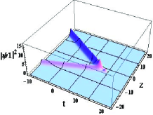
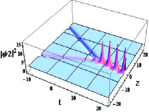
Figure 1: (color online) The evolution plot of B-DAB in the coupled system, (a) for bright soliton in $\psi_{1}$ component and (b) for dark with an AB in $\psi_{2}$ component. It is seen that the bright soliton in one field is reflected like hard wall by the AB in the other one. The dark soliton is reflected well by the AB too. The coefficients are $a_{0}=0,b_{0}=1.2,g_{1}=g_{2}=0.25,s_{1}=0.001,s_{2}=2,A_{1}=1,A_{2}=4,A_{3}=3,k_{1}=-0.5$, and $k_{2}=0.5$.

When $s_{1}\rightarrow 0$, $s_{2}\neq 0$, with the certain parameters, the bight-dark interplay with AB (B-DAB) could exist, such as Fig. 1. Particularly, Fig. 1(a) shows that one bright soliton in $\psi_{1}$ component is reflected by the other one’s density distribution. Considering that the density distribution of one component could be seen as nonlinear potential distribution for solitons in the other field, it is not hard to understand the refection effect. Correspondingly, one can observe a dark soliton collide with a AB and its shape is changed in Fig. 1(b). The reflecting inelastic collisions happen between nonlinear waves with different structures. Considering that Becker et al. have observed dark soliton collide with the B-D soliton in BEC Becker , it is believed there are some possibilities to observe the refection collision presented here.

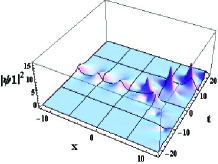
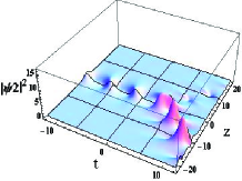
Figure 2: (color online) The evolution plot of ABs-ABs in two components coupled system. (a) for ABs soliton in $\psi_{1}$ component and (b) for ABs in $\psi_{2}$ component. It is shown that one AB collides with a AB inelastically. The coefficients are $a_{0}=0,b_{0}=1.2,g_{1}=g_{2}=0.25,s_{1}=1,s_{2}=1,A_{1}=1,A_{2}=4,A_{3}=3,k_{1}=-0.5$, and $k_{2}=0.5$.

When $s_{1}\neq 0$ and $s_{2}\neq 0$, there are many kinds of different soliton and AB appearing in the coupled system. In the nontrivial background, ABs-ABs could exist. The reflection between AB and AB can be observed, just as shown in Fig. 2(a). Two ABs could collide inelastically and then merge into one AB, as shown in Fig. 2(b). Inelastic collision for dark, bright, AB with AB could exist under some certain conditions. These characters could be used to design optical switches in nonlinear optics.

II.2 Bright-dark solitons or Akhmediev Breather interplay with Rogue Wave

It is found that when the equation of $\tau$ has double roots, namely, $\tau_{1}=-2\tau_{2}$ and $\tau_{2}=\tau_{3}$, there is a certain requirement on the spectral parameter $\lambda$. The parameter $\lambda$ which mainly determines the form of initial signals should satisfy the equation as follows

$$[3(k_{1}+k_{2})^{2}+4(C-A)]\lambda^{4}$$

$$+[4(k_{1}+k_{2})^{3}+(k_{1}+k_{2})(8C-6A)-4B]\lambda^{3}$$

$$+[4(k_{1}+k_{2})^{2}C+4C^{2}/3-A^{2}-6(k_{1}+k_{2})B]\lambda^{2}$$

$$+[4(k_{1}+k_{2})C^{2}/3-2AB]\lambda+\frac{4C^{3}}{27}-B^{2}=0,$$ (25)

where

$$A = 2(2k_{1}-k_{2})(2k_{2}-k_{1})+(k_{1}+k_{2})^{2}+9g_{1}s_{1}^{2}+9g_{2}s_{2}^{2},$$

$$B = 9g_{1}s_{1}^{2}(2k_{2}-k_{1})+(k_{1}+k_{2})(2k_{1}-k_{2})(2k_{2}-k_{1})$$

$$+9g_{2}s_{2}^{2}(2k_{1}-k_{2}),$$

$$C = (k_{1}+k_{2})^{2}-(2k_{1}-k_{2})(2k_{2}-k_{1})+9g_{1}s_{1}^{2}+9g_{2}s_{2}^{2}.$$

Under this requirement condition, the roots of $\tau$ will be given as

$$\tau_{1} = -2\tau_{2},$$ (26)

$$\tau_{2} = \tau_{3}=\frac{H_{1}(\lambda)}{H_{2}(\lambda)},$$ (27)

where

$$H_{1}(\lambda) = I[2\lambda^{3}+3(k_{1}+k_{2})\lambda^{2}+(2(2k_{1}-k_{2})(2k_{2}-k_{1})$$

$$+(k_{1}+k_{2})^{2}+9g_{1}s_{1}^{2}+9g_{2}s_{2}^{2})\lambda$$

$$+9g_{2}s_{2}^{2}(2k_{1}-k_{2})+9g_{1}s_{1}^{2}(2k_{2}-k_{1})$$

$$+(k_{1}+k_{2})(2k_{1}-k_{2})(2k_{2}-k_{1})],$$

$$H_{2}(\lambda) = 6\lambda^{2}+6(k_{1}+k_{2})\lambda+2(k_{1}+k_{2})^{2}$$

$$-2(2k_{1}-k_{2})(2k_{2}-k_{1})+18g_{1}s_{1}^{2}+18g_{2}s_{2}^{2}.$$

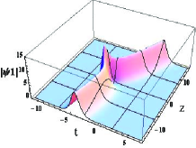
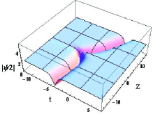
Figure 3: (color online) The evolution of B-DRW in the coupled system, (a) for one bright soliton with RW in $\psi_{1}$ component and (b) for one dark with a RW in $\psi_{2}$ component. It is shown that one dark soliton collides with RW elastically. Bright soliton are attracted by RW when being next to it. The coefficients are $a_{0}=-0.1,b_{0}=-2,g_{1}=g_{2}=0.25,s_{1}=0.01,s_{2}=2,A_{1}=1,A_{2}=4,A_{3}=3,k_{1}=-1$, and $k_{2}=0.1$.

Under these conditions, one RW appears, namely, the AB in previous part will evolve as a RW. And the RW with other type nonlinear waves solution is given in Appendix A. One can see that the form of solution partly includes rational functions. When the amplitude of one component’s background $s_{1}\rightarrow 0$, and $s_{2}>0$, the bright-dark interplay with RW (B-DRW) could be observed, such as Fig. 3. It is seen from Fig. 3(a) that the bright soliton is attracted by the RW, and collide with it, then the shape of dark soliton is unchanged after RW disappearing. When $s_{1},s_{2}>0$, the ABs emerge with RW (AB-ABRW) in each component, such as Fig. 4. One normal RW appears around $t=0$ place near $z=0$ in the first component field, and correspondingly, one dark RW emerges in the second component, which can be well shown by density distribution plot near $z=0$. Moreover, the relative location between bright or dark solitons and RW can be varied through changing the parameters $A_{j}$. Especially, when $A_{1}=0$, the AB-ABRW solution will correspond to pure one vector RW solution, shown in Fig. 4(c) and (d). In Fig. 4(d), it is shown well that the dark RW indeed exists in the second component. The similar dark RWs have been expected in mixed BEC system through numeric stimulation in Bludov2 . Namely, we could obtain analytical dark RW solution with the corresponding parameters in Fig. 4(d). Furthermore, when $A_{3}=0$, the solution will become AB-AB solution with no RW any more. The parameter $A_{2}$ just affects the place where RW appears.

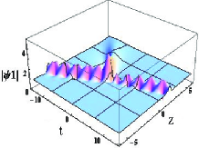
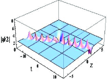
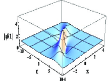
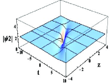
Figure 4: (color online) The plot of AB-ABRW in the coupled system, (a) for AB with a RW in $\psi_{1}$ component and (b) for AB with a dark RW in $\psi_{2}$ component. For (a) and (b), $A_{1}=1,A_{2}=4$. (c) The plot of one RW in $\psi_{1}$ component and (d) The plot of one RW in $\psi_{2}$ component. It is seen that the RW in $\psi_{2}$ component is a dark one. (c) and (d) with $A_{1}=A_{2}=0$. The other coefficients are $a_{0}=-0.53,b_{0}=2.26,g_{1}=g_{2}=0.5,s_{1}=1,s_{2}=2,A_{3}=3,k_{1}=-1$, and $k_{2}=0.1$.

On arbitrary nontrivial background, when the initial condition can be given as nearly with the certain $\lambda$ before, there are many possibilities to observe one RW interacted with bright, dark, or ABs. These interaction phenomena are impossible to be observed for scalar NLS system, for bright, dark solitons and RW can not exist simultaneously with the same conditions. The generalized nonlinear waves solution provides us a good platform to study the interactions between RW and other type nonlinear waves. On the other hand, the nonlinear wave solution partly including rational functions corresponds to a RW with other type nonlinear waves. When $A_{1}=0$, the AB-ABRW solution will be all rational form and it is one vector RW solution. One could guess that the vector RWs with no other type nonlinear waves solution could have the all rational form, just like RW solution in uncoupled system. Then, we will try to derive the all rational form solutions.

II.3 Rogue Waves with no other nonlinear waves

When $\tau$ has triple roots, we can derive the solutions with all rational functions, which usually correspond to RWs phenomena Shrira ; N.Akhmediev . Interestingly, we find that there are some certain requirements on the nontrivial backgrounds of the two components for these RWs solutions. The conditions are required as

$$g_{1}s_{1}^{2} = g_{2}s_{2}^{2},$$ (28)

$$|k_{1}-k_{2}| = \sqrt{g_{1}}s_{1},$$ (29)

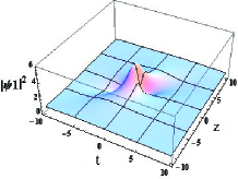
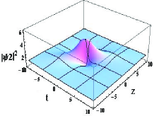
Figure 5: (color online) The evolution plot of only one RW in coupled system, (a) for one RW in $\psi_{1}$ component, (b) for one RW in $\psi_{2}$ component. The coefficients are $g_{1}=g_{2}=0.25,s_{1}=s_{2}=1,A_{1}=1,A_{2}=1,A_{3}=0,k_{1}=0.55$, and $k_{2}=0.05$.

which means that there are requirement on the nonlinear parameter and the amplitude of each component, and the difference of their wave vectors should be related with nonlinear parameter and the amplitude in a certain way. Then, RWs without any other type waves, could be observed possibly on the certain backgrounds. Meanwhile, the ideal initial conditions for the RW are presented in the coupled system. The parameter $\lambda$ which mainly determines the initial shape of vector nonlinear waves, should be set with

$$\lambda=-\frac{k_{1}+k_{2}}{2}+I\frac{3\sqrt{3}}{2}\sqrt{g_{1}}s_{1}.$$ (30)

With these certain conditions, the generic form of vector RWs could be given as

$$\psi_{1} = [1+\frac{3\sqrt{3g_{1}}s_{1}W_{1}(t,z)}{1+|u|^{2}+|v|^{2}}]s_{1}e^{i\theta_{1}(t,z)},$$ (31)

$$\psi_{2} = [1+\frac{3\sqrt{3g_{1}}s_{1}W_{2}(t,z)}{1+|u|^{2}+|v|^{2}}]s_{2}e^{i\theta_{2}(t,z)},$$ (32)

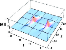
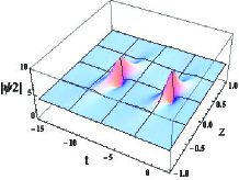
Figure 6: (color online) The evolution plot of two RWs in coupled system, (a) for two similar RWs in $\psi_{1}$ component, (b) for two similar RWs in $\psi_{2}$ component. The coefficients are $g_{1}=g_{2}=0.25,s_{1}=s_{2}=4,A_{1}=1,A_{2}=1,A_{3}=0.2,k_{1}=2.05$, and $k_{2}=0.05$.

where $u=W_{1}(t,z)\sqrt{g_{1}}s_{1}$, and $v=W_{2}(t,z)\sqrt{g_{2}}s_{2}$. The expressions of $W_{1,2}(t,z)$ are all rational functions, presented in Appendix B. Therefore, the vector waves solution could be vector RWs solution, which can be verified by the following RWs plots. When $g_{1}=g_{2}=1$, the RWs solution could become the RWs in Ling2 . When $A_{3}=0$, only one RW can be observed in both components, shown in Fig. 5. The density of them are distinct in temporal-spatial distribution, and their structures are similar to the well-known RW in single-component system. When $A_{3}\neq 0$, there are two RWs appearing in the temporal-spatial distribution, shown in Fig. 6. There are two RWs appearing in temporal-spatial distribution, which is very distinct from the higher-order RW in uncoupled system. In the uncoupled systems, it is nor possible to observe just two RWs appearing in the whole temporal-spatial distribution even for higher-order RWs Ling ; J.K.Yang .

When parameters $A_{j}$ vary, namely, the initial nonlinear waves are slightly different, the RWs properties will be changed. For example, when they are next to each other, the classical shape of RW Akhmediev ; Bludov , called eye shape, could be changed, such as fig. 7. However, the RW solution form is an ideal condition. It could be very hard to realize them precisely. From the generic solution Eq.(11) and (12), when the initial condition is a bit different from the ideal initial condition, one can observe the character of their evolution, such as Fig. 8. Comparing Fig. 6 and Fig. 8, we can know that the vector RW could be seen as a limit case of the general solution under the certain requirement condition. When the initial conditions are similar to the ideal one, the evolution of them will be close to the vector RWs. This is similar to the case that RW is the limit of AB in the uncoupled system Kibler .

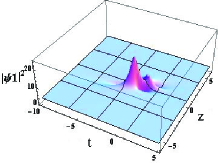
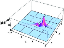
Figure 7: (color online) The evolution plot of two vector RWs in the coupled system, (a) for two different RWs in $\psi_{1}$ component, (b) for two different RWs in $\psi_{2}$ component. It is seen that dark RW could be observed in one component of the coupled system. The coefficients are $g_{1}=g_{2}=0.5,s_{1}=s_{2}=2,A_{1}=0,A_{2}=0,A_{3}=158,k_{1}=0.807$, and $k_{2}=0.05$.

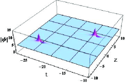
Figure 8: (Color online) The evolution of whole ABs-ABs density in the coupled system. The initial condition approaches the ideal condition for RWs, and the corresponding required backgrounds are set. It is seen that the evolution of them is close to RWs in Fig.6. The explicit coefficients are $a_{0}=-1.05,b_{0}=5.196,g_{1}=g_{2}=0.25,s_{1}=s_{2}=4,A_{1}=1,A_{2}=1,A_{3}=6,k_{1}=2.05$, and $k_{2}=0.05$.

III Possibilities to observe these vector nonlinear waves

Considering the experiments on RW in nonlinear fibers with anomalous GVD Kibler ; Solli ; Dudley , which have shown that the simple scalar NLS could describe nonlinear waves in nonlinear fibers well, we expect that these different vector nonlinear waves could be observed in two-mode nonlinear fibers. As an example, we discuss how to observe the vector RWs. One can introduce two distinct modes to a nonlinear fiber operating in the anomalous GVD regime Afanasyev ; Ueda , then the ideal condition could be given in detail. Firstly, we assume the nonlinear coefficients for the two modes are equal, namely, $g_{1}=g_{2}=0.25$. The GVD coefficients are $\sigma_{1}=\sigma_{2}=1$ in the normalized units. The spontaneous development of RW seeded from some perturbation should be on the continuous waves as the ones in Kibler ; Solli ; Dudley . Experimentally, one can use proper picosecond or nanosecond pulses which are close to the ideal continuous waves for RW development Dudley2 . The amplitudes of the backgrounds should be equal, $s_{1}=s_{2}=1$ in the normalized units. One mode laser’s frequency $k_{2}=0.05$, and the other’s is $k_{1}=k_{2}+0.5$. Then the ideal initial optical shape can be given by Eq.(19) and (20) with $\lambda=-\frac{k_{1}+k_{2}}{2}+I\frac{3\sqrt{3}}{4}$. Under these conditions, the vector RWs could be observed in the nonlinear fiber. The RW distribution is on the retarded time dimension, similar to temporal optical solitons.

On the other hand, it is well known that there are spatial optical solitons in planar waveguide. The similar conditions can be derived directly through coordinates transformation for the coupled NLS in a planar waveguide Cambournac . The RWs in multi-mode planar waveguide could be observed too. Additionally, considering the studies on two-components Bose-Einstein condensate(BEC) Doktorov ; Das ; Becker , we expect that the vector RWs could also be observed with the condition.

IV Discussion and Conclusion

In summary, we obtain B-DAB, ABs-ABs, B-DRW, AB-ABRW, and vector RWs solutions for the coupled model. The corresponding conditions for their emergence are presented explicitly. In particular, when the parameter $\lambda$, which mainly determines the shape of initial signals, satisfies Eq.(13), there are ideal initial signals existing which can evolve to one RW with other types nonlinear waves, namely, B-DRW or AB-ABRW, etc. It provides possibilities to observe interactions between RW and other type nonlinear waves. This is an interesting subject for RW studies, since these phenomena are impossible to be observed in the single-component nonlinear systems.

Just under the conditions Eq.(16) and (17), which are the certain requirements on both backgrounds of the two components, the initial condition approaching the ideal one Eq.(19) and (20) with $\lambda$ given by Eq.(18), would evolve to the vector RWs with no other type nonlinear waves. From the ideal condition, one can know that the two vector RWs can not exist when the two backgrounds are relatively static. This is very different from RW in the uncoupled system, for which there is no requirement on nontrivial background Kibler . Additionally, dark RW, predicted in mixed BEC system through numeric stimulation in Bludov2 , is observed analytically here. Moreover, one possible way to observe vector RWs in a two-mode nonlinear fiber is presented here.

Recently, the higher-order modulation instability with RWs has been observed in nonlinear fiber optics in Erkintalo . There are many possibilities to observe similar phenomena in coupled nonlinear fiber system. We will continue to study this subject in the future work.

Appendix A: The analytic form for B-DRW AND AB-ABRW WAVES

The RW with other type solitons could be derived as

$$\psi_{1} = \psi_{10}-\frac{1}{\sqrt{g_{1}}}\frac{i(\lambda-\bar{\lambda})\Phi_{1}\bar{\Phi}_{2}}{|\Phi_{1}|^{2}+|\Phi_{2}|^{2}+|\Phi_{3}|^{2}},$$ (33)

$$\psi_{2} = \psi_{20}-\frac{1}{\sqrt{g_{2}}}\frac{i(\lambda-\bar{\lambda})\Phi_{1}\bar{\Phi}_{3}}{|\Phi_{1}|^{2}+|\Phi_{2}|^{2}+|\Phi_{3}|^{2}},$$ (34)

where

$$\Phi_{1}[t,z] = (\Phi_{01}+\Phi_{02}+\Phi_{03})$$

$$\times\text{Exp}\left[\frac{I}{3}(\theta_{1}[t,z]+\theta_{2}[t,z])\right],$$

$$\Phi_{2}[t,z] = (\frac{-\sqrt{g_{1}}s_{1}}{\tau_{1}-I\lambda/3-I(2k_{1}-k_{2})/3}\Phi_{01}[t,z]$$

$$+\frac{-\sqrt{g_{1}}s_{1}}{\tau_{2}-I\lambda/3-I(2k_{1}-k_{2})/3}\Phi_{02}[t,z]$$

$$+\frac{-\sqrt{g_{1}}s_{1}-\frac{-\sqrt{g_{1}}s_{1}}{\tau_{2}-I\lambda/3-I(2k_{1}-k_{2})/3}}{\tau_{2}-I\lambda/3-I(2k_{1}-k_{2})/3}\Phi_{03}[t,z])$$

$$\times\text{Exp}\left[\frac{I}{3}(\theta_{2}[t,z]-2\theta_{1}[t,z])\right],$$

$$\Phi_{3}[t,z] = (\frac{-\sqrt{g_{2}}s_{2}}{\tau_{1}-I\lambda/3-I(2k_{2}-k_{1})/3}\Phi_{01}[t,z]$$

$$+\frac{-\sqrt{g_{2}}s_{2}}{\tau_{2}-I\lambda/3-I(2k_{2}-k_{1})/3}\Phi_{02}[t,z]$$

$$+\frac{-\sqrt{g_{2}}s_{2}-\frac{-\sqrt{g_{2}}s_{2}}{\tau_{2}-I\lambda/3-I(2k_{2}-k_{1})/3}}{\tau_{2}-I\lambda/3-I(2k_{2}-k_{1})/3}\Phi_{03}[t,z])$$

$$\times\text{Exp}\left[\frac{I}{3}(\theta_{1}[t,z]-2\theta_{2}[t,z])\right],$$

and

$$\Phi_{01} = A_{1}\text{Exp}[\tau_{1}t+I\tau_{1}^{2}z+2(\lambda-k_{1}-k_{2})\tau_{1}z/3],$$

$$\Phi_{02} = (A_{3}t+2A_{3}I\tau_{2}z+2/3A_{3}(\lambda-k_{1}-k_{2})z+A_{2})$$

$$\times\text{Exp}[\tau_{2}t+I\tau_{2}^{2}z+2(\lambda-k_{1}-k_{2})\tau_{2}z/3],$$

$$\Phi_{03} = A_{3}\text{Exp}[\tau_{2}t+I\tau_{2}^{2}z+2(\lambda-k_{1}-k_{2})\tau_{2}z/3].$$

Between the above expressions, the parameter $\lambda$ is the solution of Eq.(13).

Appendix B: The analytic form for $W_{1,2}$

The expressions of $W_{1,2}$ are

$$W_{1,2}(t,z) = \frac{1}{K_{1,2}}+\frac{1}{K_{1,2}^{2}}+\frac{P_{1,2}(t,z)}{Q(t,z)}$$

where

$$K_{1} = \frac{i(k_{1}-k_{2})}{2}-\frac{\sqrt{3g_{1}}s_{1}}{2},$$

$$K_{2} = \frac{i(k_{2}-k_{1})}{2}-\frac{\sqrt{3g_{1}}s_{1}}{2},$$

and

$$Q(t,z) = \frac{1}{2}A_{3}t^{2}+\frac{2}{9}(\lambda-k_{1}-k_{2})^{2}A_{3}z^{2}+(A_{2}+A_{3})t$$

$$+\frac{2}{3}(\lambda-k_{1}-k_{2})(A_{2}+A_{3})z+iA_{3}z$$

$$+\frac{2}{3}(\lambda-k_{1}-k_{2})A_{3}tz+A_{1}+A_{2}+A_{3},$$

$$P_{1,2}(t,z) = \frac{A_{3}}{K_{1,2}^{3}}-\frac{1}{K_{1,2}^{2}}M(t,z),$$

$$M(t,z) = \frac{1}{2}A_{3}t^{2}+\frac{2}{9}(\lambda-k_{1}-k_{2})^{2}A_{3}z^{2}+A_{2}t$$

$$+\frac{2}{3}(\lambda-k_{1}-k_{2})A_{2}z+iA_{3}z$$

$$+\frac{2}{3}(\lambda-k_{1}-k_{2})A_{3}tz+A_{1}.$$

Between the above expressions, the parameter $\lambda$ is given by Eq.(18).

References

- (1) K. E. Strecker,G.B. Partridge, A.G. Truscott, R.G. Hulet , ”Formation and propagation of matter-wave soliton trains ”, Nature (London) 417, 150 (2002); T.C. Hernandez, V.E. Villargan, V.N. Serkin, GM Aguero, TL Belyaeva, MR Pena, and LL Morales, ”Dynamics of solitons in the model of nonlinear Schrödinger equation with an external harmonic potential: I. Bright solitons” , Quantum Electron. 35, 778-786 (2005).
- (2) P. G. Kevrekidis, G. Theocharis, D.J. Frantzeskakis,Boris A. Malomed, ”Feshbach Resonance Management for Bose-Einstein Condensates ”, Phys. Rev. Lett. 90, 230401 (2003); K.H. Han, H.J. Shin, ”Nonautonomous integrable nonlinear Schrödinger equations with generalized external potentials”, Journ. Phys. A 42, 335202 (2009).
- (3) L. Khaykovich, F. Schreck, G. Ferrari, T. Bourdel, J. Cubizolles, L. D. Carr, Y. Castin, C. Salomon, ”Formation of a Matter-Wave Bright Soliton”, Science 296, 1290 (2002).
- (4) W.B. Cardoso, A.T. Avelar, D. Bazeia, ”Modulation of breathers in cigar-shaped Bose CEinstein condensates ”, Phys. Lett. A 374, 2640-2645 (2010).
- (5) S. Burger, K. Bongs, S. Dettmer, W. Ertmer, and K. Sengstock , ”Dark Solitons in Bose-Einstein Condensates ”, Phys. Rev. Lett. 83, 5198 (1999).
- (6) J. Denschlag, J.E. Simsarian, D.L. Feder,Charles W. Clark, L. A. Collins, J. Cubizolles, L. Deng, E. W. Hagley, K. Helmerson, W. P. Reinhardt, S. L. Rolston, B. I. Schneider, W. D. Phillips, ”Generating Solitons by Phase Engineering of a Bose-Einstein Condensate”, Science 287, 97 (2000).
- (7) T. Busch and J. R. Anglin, ”Motion of dark solitons in trapped Bose-Einstein condensates ”, Phys. Rev. Lett. 84, 2298 (2000).
- (8) C.K. Law, C.M. Chan, P.T. Leung, and M.-C. Chu , ”Motional Dressed States in a Bose-Einstein Condensate: Superfluidity at Supersonic Speed”, Phys. Rev. Lett. 85, 1598 (2000).
- (9) B.P. Anderson, P.C. Haljan, C.A. Regal,D. L. Feder, L. A. Collins, C. W. Clark, and E. A. Cornell , ”Watching Dark Solitons Decay into Vortex Rings in a Bose-Einstein Condensate ”, Phys. Rev. Lett. 86, 2926 (2001).
- (10) B. Wu, J. Liu, Q. Niu, ”Controlled generation of dark solitons with phase imprinting ”, Phys. Rev. Lett. 88, 034101 (2002).
- (11) N. Akhmediev, A. Ankiewicz, Solitons, Nonlinear Pulses and Beams (Chapman and Hall, 1997; N. Akhmediev, J.M. Soto-Crespo,and A. Ankiewicz, ”Extreme waves that appear from nowhere: On the nature of rogue waves”, Phys. Lett. A 373, 2137-2145 (2009).
- (12) V.I. Shrira, V.V. Geogjaev, ”What makes the Peregrine soliton so special as a prototype of freak waves? ”, J. Eng. Math. 67, 11-22 (2010).
- (13) B. Kibler, J. Fatome, C. Finot, G. Millot, F. Dias, G. Genty, N. Akhmediev, J. M. Dudley, ”The Peregrine soliton in nonlinear fibre optics”, Nature Phys. 6, 790 (2010).
- (14) Q.H. Park, and H.J. Shin, ”Systematic construction of multicomponent optical solitons ”, Phys. Rev. E 61, 3093 (2000).
- (15) P. Kockaert, P. Tassin, G.V. Sande, I. Veretennicoff, and M. Tlidi , ”Negative diffraction pattern dynamics in nonlinear cavities with left-handed materials ”, Phys. Rev. A 74, 033822 (2006).
- (16) T. Kanna, M. Lakshmanan, ”Exact Soliton Solutions, Shape Changing Collisions, and Partially Coherent Solitons in Coupled Nonlinear Schrödinger Equations”, Phys. Rev. Lett. 86, 5043 (2001).
- (17) M. Vijayajayanthi, T. Kanna, and M. Lakshmanan, ”Bright-dark solitons and their collisions in mixed N-coupled nonlinear Schrödinger equations”, Phys. Rev. A 77, 013820 (2008); M. Vijayajayanthi, T. Kanna and M. Lakshmanan, ”Multisoliton solutions and energy sharing collisions in coupled nonlinear Schrödinger equations with focusing, defocusing and mixed type nonlinearities”, Europ. Phys. Journ. - Special Topics 173, 57-80 (2009).
- (18) L.C. Zhao, S.L. He, ”Matter wave solitons in coupled system with external potentials”, Phys. Lett. A 375, 3017-3020 (2011).
- (19) C. Becker, S. Stellmer, P.S. Panahi, S. Dorscher, M. Baumert, Eva-Maria Richter, Jochen Kronjager, Kai Bongs,Klaus Sengstock, ”Oscillations and interactions of dark and dark Cbright solitons in Bose CEinstein condensates ”, Nature phys. 4, 496-501 (2008).
- (20) M.G. Forest, S.P. Sheu, and P.C. Wright, ”On the construction of orbits homoclinic to plane waves in integrable coupled nonlinear Schrödinger systems ”, Phys. Lett. A 266, 24 (2000).
- (21) B.L. Guo, L.M. Ling, ”Rogue Wave, Breathers and Bright-Dark-Rogue Solutions for the Coupled Schrödinger Equations ”, Chin. Phys. Lett. 28, 110202 (2011).
- (22) F. Baronio, A. Degasperis, M. Conforti, and S. Wabnitz, ”Solutions of the Vector Nonlinear Schrödinger Equations: Evidence for Deterministic RogueWaves”, Phys. Rev. Lett. 109, 044102 (2012).
- (23) B. Crosignani and P. Di Porto, ”Soliton propagation in multimode optical fibers”, Opt. Lett. 6, 329 (1981); V. V. Afanasyev, Yu. S. Kivshar, V. V. Konotop, V. N. Serkin, ”Dynamics of coupled dark and bright optical solitons”, Opt. Lett. 14, 805 (1989).
- (24) M. Haelterman and A. Sheppard, ”Bifurcation phenomena and multiple soliton-bound states in isotropic Kerr media ”, Phys. Rev. E 49, 3376 (1994).
- (25) Y.V. Bludov, V.V. Konotop, and N. Akhmediev, Eur. Phys. J. Special Topics 185, 169-180 (2010).
- (26) B.L. Guo, L.M. Ling, Q. P. Liu , ”Nonlinear Schrödinger equation: Generalized Darboux transformation and rogue wave solutions ”, Phys. Rev. E 85, 026607 (2012).
- (27) Y. Ohta, J.K. Yang, ”General high-order rogue waves and their dynamics in the nonlinear Schrödinger equation”, Proc. R. Soc. A 468, 1716-1740 (2012).
- (28) Y.V. Bludov, V.V. Konotop, and N. Akhmediev, ”Matter rogue waves ”, Phys. Rev. A 80, 033610 (2009).
- (29) N. Akhmediev, A. Ankiewicz, M. Taki, ”Waves that appear from nowhere and disappear without a trace ”, Phys. Lett. A 373, 657-678 (2009).
- (30) D.R. Solli, C.Ropers, P.Koonath, B.Jalali, ”Optical rogue waves ”, Nature 450, 1054-1057 (2007).
- (31) J. M. Dudley, G. Genty, B. J. Eggleton, ”Harnessing and control of optical rogue waves in supercontinuum generation,” Opt. Express 16, 3644-3651 (2008).
- (32) Tetsuji Ueda and William L. Lath, ”Dynamics of coupled solitons in nonlinear optical fibers”, Phys. Rev. A 42, 563 (1990).
- (33) J. M. Dudley, G. Genty, F. Dias, B. Kibler, N. Akhmediev, ”Modulation instability, Akhmediev Breathers and continuous wave supercontinuum generation”, Opt. Express 17, 21497-21508 (2009).
- (34) C. Cambournac, T. Sylvestre, H. Maillotte, B. Vanderlinden, P. Kockaert, Ph. Emplit, and M. Haelterman , ”Symmetry-breaking instability of multimode vector solitons ”, Phys. Rev. Lett. 89, 083901 (2002).
- (35) P. Das, T.S. Raju, U. Roy, and Prasanta K. Panigrahi, ”Sinusoidal excitations in two-component Bose-Einstein condensates in a trap”, Phys. Rev. A 79, 015601 (2009).
- (36) E. V. Doktorov, V. M. Rothos, Y. S. Kivshar, ”Full-time dynamics of modulational instability in spinor Bose-Einstein condensates”, Phys. Rev. A 76, 013626 (2007).
- (37) M. Erkintalo, K. Hammani, B. Kibler,C. Finot, N. Akhmediev, J. M. Dudley, and G. Genty, ”Higher-Order Modulation Instability in Nonlinear Fiber Optics”, Phys. Rev. Lett. 107, 253901 (2011).