Outer Billiards with Contraction: Attracting Cantor Sets

Abstract

We consider the outer billiards map with contraction outside polygons. We construct a 1-parameter family of systems such that each system has an open set in which the dynamics is reduced to that of a piecewise contraction on the interval. Using the theory of rotation numbers, we deduce that every point inside the open set is asymptotic to either a single periodic orbit (rational case) or a Cantor set (irrational case). In particular, we deduce existence of an attracting Cantor set for certain parameter values. Moreover, for a different choice of a 1-parameter family, we prove that the system is uniquely ergodic; in particular, the entire domain is asymptotic to a single attractor.

1 Introduction

Let $P$ be a convex polygon in the plane and $0<\lambda<1$ be a real number. Given a pair $(P,\lambda)$, we define the outer billiards with contraction map $T$ as follows. For a generic point $x\in\mathbb{R}^{2}\backslash P$, we can find a unique vertex $v$ of $P$ such that $P$ lies on the left of the ray starting from $x$ and passing through $v$. Then on this ray, we pick a point $y$ that lies on the other side of $x$ with respect to $v$ and satisfies $|xv|:|vy|=1:\lambda$. We define $Tx=y$ (Figure 1). The map $T$ is well-defined for all points on $\mathbb{R}^{2}\backslash P$ except for points on the union of singular rays extending the sides of $P$.

Figure 1: Outer billiards with contraction

The case $\lambda=1$ corresponds to the usual outer billiards map. This map has been studied by many people [14, 21, 19, 22, 11, 20]; [23] is a classical reference. We first point out that while it is highly nontrivial to show that the outer billiards map can have unbounded orbits for certain polygons [18], it is straightforward to see that with any contraction $0<\lambda<1$, every orbit is bounded. While the system itself has several interesting behavior, we state a few motivations to study outer billiards with contraction.

• Electrical engineering: It is known that the outer billiards map is connected to certain systems from electrical engineering [5, 7, 6]. Then, applying contraction may model more realistic systems in which dissipation of energy occurs; see [4].

• Application to the outer billiards map: By considering the limit $\lambda\rightarrow 1$, one gains some information regarding the structure of the set of periodic points of the outer billiards map. See [12] for some illustrations of this phenomenon.

• An analogy of inner billiards with contraction: Contractive inner billiards have been studied, for example, in [9, 10]. Then it is natural to consider the outer billiards counterpart; we have learned this motivation from [8].

Recent papers [3, 15] discuss a few more motivations to study piecewise contractions in general.

Experiment suggests that when we pick $P$ and $\lambda$ at random, (1) there are only finitely many periodic orbits and (2) all orbits are asymptotically periodic. Indeed, these two phenomena are expected from a generic piecewise contracting map; [3, 15, 1] prove exactly results of this kind. In [3], authors consider a large class of piecewise affine contractions on the plane and show that for almost every choice of parameters, any orbit is attracted to a periodic one. In [15, 1], authors consider piecewise contractions on the interval and show that the number of periodic orbits is always finite, and asymptotic periodicity for almost every choice of parameters by adding a smoothness assumption on each piece. We point out special cases where regularity statements (1) and (2) above can be explicitly proved: When $P$ is either a triangle, parallelogram, or a regular hexagon, then for each $0<\lambda<1$, there exists only finitely many periodic orbits for $T$ and all orbits are asymptotically periodic. Proofs of this fact are carried out in [12, 8], using different methods.

In a sense, our goal will be the opposite to that of aforementioned papers. The main result of this paper is the following.

Theorem.

There exists uncountably many pairs $(P,\lambda)$ for which $T$ has a Cantor set as an attractor.

It will turn out that the set of parameter values where we can show existence of such Cantor sets also have zero measure in the parameter space. As far as we know, it is the first explicit description of a 2-dimensional system (that is not a direct product of two 1-dimensional systems) having an attracting Cantor set. An outline is as follows:

1. We find 1-parameter family of pairs $(P,\lambda)$ which has a thin forward invariant rectangle. (Definition 3.1, Lemma 3.1)

2. The thin rectangle is divided into two rectangles, and the dynamics on each rectangle is reduced to a one-dimensional piecewise affine contraction. (Definition 3.2, Lemma 3.2)

3. We show that the rotation numbers of these maps are well-defined and vary continuously with the parameter. (Lemma 3.3)

4. If this rotation number is irrational, there must be an attracting Cantor set. (Theorem 1)

5. Finally, we conclude the proof by show that the rotation number is non-constant as a function of the parameter by computing 2 examples. (Theorem 2)

A brief theory of rotation numbers for discontinuous circle maps is given in Section 2, and the above outline is carried out in Section 3. In Section 4, we consider more general parameter values and discuss global behavior of the system. In particular, we show that there are cases where the attracting Cantor set is the global attractor.

2 Rotation Theory for Discontinuous Circle Maps

Recall that the rotation number for a circle homeomorphism $f:S^{1}\rightarrow S^{1}$ is defined by

$$\rho(F)=\lim_{n\rightarrow\infty}\frac{F^{n}(x)-x}{n}$$ (1)

where $F$ is any lift of $f$ into a homeomorphism of $\mathbb{R}$ and $x$ is an arbitrary real number. Once we fix $F$, this limit exists and independent on $x$. If we have two lifts $F_{1}$ and $F_{2}$, then $\rho(F_{1})-\rho(F_{2})$ is an integer so that the rotation number of $f$, $\rho(f)$ is uniquely determined mod 1. Then, $\rho(f)$ is rational if and only if $f$ has a periodic point. On the other hand, when $\rho(f)$ is irrational, the $\omega$-limit set of a point (which is independent on the point) is either the whole circle or a Cantor set.

Rhodes and Thompson, in [16, 17], develops a theory of rotation number for a large class of functions $f:S^{1}\rightarrow S^{1}$. We only state the results that we need. A map (not necessarily continuous) $f:S^{1}\rightarrow S^{1}$ is in class $\mathcal{S}$ if and only if it has a lift $F:\mathbb{R}\rightarrow\mathbb{R}$ such that $F$ is strictly increasing and $F(x+1)=F(x)+1$ for all $x\in\mathbb{R}$. Now given such a lift $F$, since it is strictly increasing, we can define $F^{-}$ and $F^{+}$, where they are continuous everywhere from the left and from the right, respectively and coincide with $F$ whenever $F$ is continuous. Then we consider the filled-graph of $F$ defined by

$$\Gamma(F):=\{(x,y)|0\leq x\leq 1,\,F^{-}(x)\leq y\leq F^{+}(x)\}$$

which is simply the graph of $F$ where all the jumps are filled with vertical line segments. We have restricted the set to the region $0\leq x\leq 1$ to make it compact. We will consider the Hausdorff metric on the collection of $\Gamma(F)$ where $F$ is some lift of $f\in\mathcal{S}$.

In terms of this theory, it does not matter how maps are defined at points of discontinuity. Therefore, we follow the convention of [2]; for maps in $\mathcal{S}$, a periodic point (or periodic orbit) of $f$ will mean a periodic point (or periodic orbit) of a map which might differ from $f$ at some points of discontinuity. With this convention, we have the following theorems.

Theorem.

[16] The rotation number $\rho(f)$ is well-defined for $f\in\mathcal{S}$ up to mod 1 by the equation 1 where $F$ is any strictly increasing degree 1 lift of $f$. This number does not change if we redefine $f$ at its points of discontinuity. Moreover, $\rho(f)$ is rational if and only if $f$ has a periodic point.

Theorem.

[17] Let $F_{\theta}$ be a family of strictly increasing degree 1 functions $\mathbb{R}\rightarrow\mathbb{R}$ for $\theta\in[0,1]$. If $\Gamma(F_{\theta})\rightarrow\Gamma(F_{0})$ as $\theta\rightarrow 0$ in the Hausdorff topology, then $\rho(F_{\theta})\rightarrow\rho(F_{0})$.

Finally, regarding the $\omega$-limit set we refer to [2].

Theorem.

[2] If $f\in\mathcal{S}$ has a rational rotation number $p/q$, $\omega(x)$ gives a $q$-periodic orbit of $f$ for all $x\in S^{1}$. If $f$ has an irrational rotation number, $\omega(x)=\omega(y)$ for all $x,y\in S^{1}$ and it is either $S^{1}$ or homeomorphic to a Cantor set.

3 Attracting Cantor Sets

We begin with some general discussion of the system. When $P$ is a convex $n$-gon, with clockwisely oriented vertices $A_{1},...,A_{n}$, then let $S$ denote the union of $n$ singular rays $\overrightarrow{A_{1}A_{2}},...,\overrightarrow{A_{n-1}A_{n}},\overrightarrow{A_{n}A_{1}}$ where $T$ is not well-defined. Then map $T$ is well-defined indefinitely on the set $X:=\mathbb{R}^{2}\backslash\big{(}P\cup(\cup_{i=0}^{\infty}T_{\lambda}^{-i}S)\big{)}$, which has full measure on $\mathbb{R}^{2}\backslash P$. We say that an ordered set of points $(w_{1},...,w_{n})$ is a periodic orbit if for each $1\leq i\leq n$, either $w_{i}\in X$ and $Tw_{i}=w_{i+1}$ (where $w_{n+1}:=w_{1})$ or $w_{i}\in S$ and $w_{i+1}$ is one of (at most) two natural choices for $Tw_{i}$ which would make $T$ continuous from one side of the plane. Note that this generalized notion of a periodic orbit is consistent with the one described in the previous section.

Now we proceed to the description of our 1-parameter family of systems, with parameter $a$ varying in the closed interval $[0.3,0.6]$. The polygon $P$ will be the quadrilateral with vertices $A=(0,1)$, $B=(a,1)$, $C=(1,0.2)$, and $D=(0,0)$. The contraction factor $\lambda$ will be equal to 0.8, independent on $a$. For simplicity, we will write $\lambda$ instead of $0.8$. We also set $\mu=\lambda^{-1}$

Let us describe how the points in Figure 2 are constructed. To begin with, the point $F$ (respectively, $G$) lies on the line $\overleftrightarrow{AD}$ (resp. $\overleftrightarrow{BC}$) and satisfies $|\overline{AD}|:|\overline{DF}|=\lambda$ (resp. $|\overline{BC}|:|\overline{CG}|=1:\mu$). Then we see that the line $\overleftrightarrow{FG}$ is parallel to the line $\overleftrightarrow{AB}$. Then the point $E$ (resp. $H$) is the intersection of the line $\overleftrightarrow{AB}$ with $\overleftrightarrow{DG}$ (resp. $\overleftrightarrow{AB}$ with $\overleftrightarrow{FC}$). Finally, we pick the point $I^{\prime}$ on the segment $\overline{BH}$ which satisfies $|\overline{AB}|:|\overline{BI^{\prime}}|=\lambda:1$. Then we define $I$ to be the point on the segment $\overline{EA}$ such that $T^{2}I=I^{\prime}$.

Figure 2: Constructing extra points

We say that a region $Y\subset\mathbb{R}^{2}\backslash P$ is forward invariant if for each $x\in Y\cap X$, there exists $n>0$ such that $T^{n}x\in Y$.

Definition 3.1 (The Invariant Rectangles).

Let $(-l,1)$ be the coordinates for the point $E$. For sufficiently small $\epsilon>0$, we define $R_{1}$ as the closed filled-in rectangular region with vertices $(0,1)$, $(0,1+\epsilon^{2})$, $(-l+\epsilon,1)$, and $(-l+\epsilon,1+\epsilon^{2})$. Then reflect $R_{1}$ over $\overline{EA}$ to obtain $R_{2}$.

Lemma 3.1 (Invariance).

For sufficiently small $\epsilon>0$,

1. any point in $R_{1}$ has a forward interate in $R_{2}$ and vice versa. In particular, $R_{1}$ and $R_{2}$ are forward invariant regions, and

2. Set $\hat{f}$ and $\hat{g}$ as the first-return maps to regions $R_{1}$ and $R_{2}$, respectively Then these maps preserve the vertical partition of the rectangles; that is, if two points in $R_{1}$ (or in $R_{2}$) have the same $x$-coordinates, there forward iterates also have the same $x$-coordinates. Moreover, given a point in $R_{1}$ (resp. $R_{2}$), the sequence of $y$-coordinates formed by its $\hat{f}$-iterates ($\hat{g}$-iterates, resp.) converges to $1$, which is the $y$-coordinate of $\overline{EA}$.

The dynamics is not well-defined at certain points on $R_{1}\cup R_{2}$. For example, the segment obtained as the intersection of those two rectangles is singular. We always follow the convention that the dynamics at such points is defined to be the one that makes $T$ continuous in the region we are looking at. That is, the segment $\overline{BH}$, viewed as a subset of $T^{2}(R_{1})$, will reflect on the vertex $A$, but viewed as a subset of $T^{2}(R_{2})$, it will reflect on the vertex $B$.

Proof.

The line passing through the point $I$ and perpendicular to $\overline{EA}$ divides $R_{2}$ into two closed rectangles $R_{2l}$ (on the left) and $R_{2r}$ (on the right). The first claim is proved with the following three crucial containments: (see Figures 3 and 4)

• $T^{3}R_{1}\subset R_{2}$

• $T^{4}R_{2l}\subset R_{2r}$

• $T^{3}R_{2r}\subset R_{1}$ (which together with $T^{3}R_{1}\subset R_{2}$ implies $T^{6}R_{2r}\subset R_{2}$)

Let us prove above containments. First we note that for $\epsilon>0$ small, every points on the image $T(R_{1}\cup R_{2})$ lies below the line $\overleftrightarrow{BC}$ so that entire rectangle $T(R_{1}\cup R_{2})$ reflects on the vertex $C$ and not $B$ (this is the only place we need $\epsilon$ to be small). Hence $T^{2}(R_{1}\cup R_{2})$ is another rectangle intersecting $\overline{BH}$. Now, to prove $T^{3}R_{1}\subset R_{2}$, it is enough to check that the $x$-coordinate of the point $H$, when reflected and contracted by $\lambda$ at the vertex $A$, is contained in the segment $R_{1}\cap R_{2}$. This holds for all $0.3\leq a\leq 0.6$. Next, it is obvious from $T^{3}R_{1}\subset R_{2}$ that $T^{3}R_{2r}\subset R_{1}$. Lastly, it is another calculation to show that $T^{4}R_{2l}\subset R_{2r}$ for all $0.3\leq a\leq 0.6$.

Next, since each iterate of $T$ contracts the distance between the point and either the line $\overleftrightarrow{AB}$ or $\overleftrightarrow{FG}$ by $\lambda$ and it takes for points in $R_{1}\cup R_{2}$ at least $T^{3}$ to return to $R_{1}\cup R_{2}$, the convergence towards the segment $\overline{EA}$ is exponential. ∎

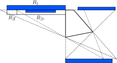
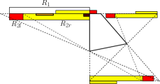
Figure 3: Forward iterates of $R_{1}$; $T^{3}R_{1}\subset R_{2}$ for $a=0.3$ (left) and $a=0.6$ (right)

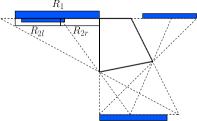
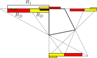
Figure 4: Forward iterates of $R_{2}$; $T^{4}R_{2l}\subset R_{2r}$ and $T^{6}R_{2r}\subset R_{2}$ for for $a=0.3$ (left) and $a=0.6$ (right)

Definition 3.2 (One-dimensional Systems).

Let $I_{\epsilon}$ be the interval obtained by the intersection $R_{1}\cap R_{2}$. Given a point $p=(p_{1},1)$ on the interval $I_{\epsilon}$, pick $\delta>0$ small enough that $(p_{1},1+\delta)\in R_{1}$. Vertically project $\hat{f}(p_{1},1+\delta)$ onto $I_{\epsilon}$ and define it to be $f(p)$. This map $f:I_{\epsilon}\rightarrow I_{\epsilon}$ is well-defined independent on the choice of $\delta$. Note that if we have two different $\epsilon_{1}>\epsilon_{2}$, the map $f$ coincides on the intersection $I_{\epsilon_{1}}\cap I_{\epsilon_{2}}=I_{\epsilon_{1}}$. Therefore we take the limit $\epsilon\rightarrow 0^{+}$ and then $f$ is well-defined on the segment $\overline{EA}$. Similarly, using $\hat{g}$ we define $g$ on the segment $\overline{EA}$.

That is, the map $f$ ($g$, resp.) describes the dynamics of the upper rectangle $R_{1}$ (the lower rectangle $R_{2}$, resp.).

Lemma 3.2 (Reduction to One-dimensional Systems).

Let $p\in X\cap(R_{1}\cup R_{2})$. Then $\omega_{T}(p)\cap(R_{1}\cup R_{2})=\omega_{T}(p)\cap\overline{EA}=\omega_{f}(p^{\prime})\cup\omega_{g}(p^{\prime\prime})$, where $p^{\prime}$ and $p^{\prime\prime}$ are vertical projections of some forward $T$-iterates of $p$ which lies on $R_{1}$ and $R_{2}$, respectively.

Proof.

Let $x\in\omega_{T}(p)\cap\overline{EA}$. We have a sequence $T^{n_{1}}p,T^{n_{2}}p,...$ on $R_{1}\cup R_{2}$ which converges to $x$. Then infinitely many of them lie on $R_{1}$ and hence we get a subsequence which we can as well write in the form $\hat{f}^{m_{1}}p,\hat{f}^{m_{2}}p,...$. That is, $x\in\omega_{\hat{f}}(p)$. We have $f\circ\mathrm{Proj}=\mathrm{Proj}\circ\hat{f}$ where $\mathrm{Proj}$ is the projection map from $R_{1}\cup R_{2}$ onto $\overline{EA}$. Therefore, $x\in\omega_{f}(p^{\prime})$.

Let $x\in\omega_{f}(p^{\prime})$. By our assumption, there is a point $p\in X\cap(R_{1}\cup R_{2})$ that $p^{\prime}$ is the projection of some $T^{n}p\in R_{1}$. From the sequence of points $f^{n_{1}}(p^{\prime}),f^{n_{2}}(p^{\prime}),...$ that converges to $x$, we get a sequence of points $\hat{f}^{m_{1}}p,\hat{f}^{m_{2}}p,$… that also converges to $x$. Since $\hat{f}$ is just some iterates of $T$, we get $x\in\omega_{T_{\lambda}}(p)\cap\overline{EA}$.

Notice that this result still holds when we view $f$ and $g$ as discontinuous circle maps. This identification may create new periodic orbits which cannot be obtained from the dynamics of $T$, but such a periodic orbit, even when it exists, will not attract any regular points as $\omega$-limit sets remain the same. ∎

Now we prove an important lemma which shows that the 1-dimensional systems $g$ and $f$ have well-defined rotation numbers.

Lemma 3.3 (Rotation Number).

The rotation number of $g$ and $f$ are well-defined mod 1. Moreover, these rotation numbers vary continuously in the parameter $a$.

Proof.

We apply an orientation preserving affine map from the interval $\overline{EA}$ onto $[0,1]$ so that $g$ and $f$ are now maps $[0,1]\rightarrow[0,1]$. Then it is a straightforward computation to show that

$$g(x)=\begin{cases}\lambda^{4}(x-1+h/l)+1&0<x<1-h/l\\ \lambda^{6}(x-1)+(1-y/l)&1-h/l<x\leq 1\end{cases}$$ (2)

where

$$l =\mu+(1-a)\mu^{2}=|\overline{EA}|$$ (3)

$$h =l-a\mu^{3}=|\overline{IA}|$$ (4)

$$y =\lambda(1+\lambda)(1+a\lambda^{2}-\lambda^{3})$$ (5)

are positive constants. For the rotation number of $g$ to be well-defined, we only need to check that it is injective (as it is strictly increasing on each interval of continuity), which is equivalent to showing that two sets $T^{4}R_{2l}$ and $T^{6}R_{2r}$ are disjoint subsets of $R_{2}$ (see Figure 4 and also Figure 5 for visual verifications of this fact). This is again equivalent to checking $\lim_{x\rightarrow 0^{+}}g(x)>g(1)$ which is proved by a simple computation. We then define a lift

$$G(x)=\begin{cases}g(x)&0<x\leq 1-h/l\\ g(x)+1&1-h/l<x\leq 1\end{cases}$$

on $(0,1]$ and extend to $\mathbb{R}$ by $G(x+1)=G(x)+1$.

Next we argue continuity of the rotation number. Given five parameters $\lambda_{1}$, $\lambda_{2}$, $c_{1}$, $c_{2}$, and $t$, which all lie in $(0,1)$, we can associate the following function:

$$H(x)=\begin{cases}\lambda_{1}x+c_{1}&0<x\leq t\\ \lambda_{2}x+c_{2}+1&t<x\leq 1\end{cases}.$$

For each $0.3\leq a\leq 0.6$, $G$ takes above form for appropriate parameters. If we fix four parameters and vary the remaining one continuously, (the closure of) the filled-graph of $H$ varies continuously in the Hausdorff topology. It is clear that varying $a$ continuously moves five parameters continuously, which implies that the rotation number varies continuously as well.

Similarly, $f$ is a piecewise linear contraction with slopes $\lambda^{10}$ and $\lambda^{6}$. A similar sequence of computations shows that $f$ is injective and that the rotation number $\rho(f)$ is well-defined as well. ∎

Theorem 1.

For each $0.3\leq a\leq 0.6$, when $\rho(g)$ is rational, there is a unique attracting $T$-periodic orbit such that every orbit starting from $X\cap(R_{1}\cup R_{2})$ is asymptotic to, and when $\rho(g)$ is irrational, every orbit starting from $X\cap(R_{1}\cup R_{2})$ is asymptotic to a unique invariant Cantor set.

Proof.

We have seen that any point in $R_{1}$ has an iterate in $R_{2}$ and vice versa. Hence we know that a $f$-periodic orbit will induce a $g$-periodic orbit and vice versa. Therefore, $\rho(f)$ is rational if and only if $\rho(g)$ is rational.

Now assume that $\rho(g)$ is rational. Then the limit set of any point for $f$ and $g$ is finite, so by Lemma 3.2, the limit set $\omega_{T}(p)$ for $p\in X\cap(R_{1}\cup R_{2})$ is finite as well; this gives an attracting periodic orbit for $T$. Now given a periodic orbit for $T$ intersecting $R_{1}\cup R_{2}$. By restriction, we obtain a periodic orbit of $g$. Now we claim that there cannot be more than two periodic orbits. This is geometrically clear in the case when $\rho(g)=0$ (see Figure 5). So assume that the denominator of $\rho(g)$ is $r\geq 2$. The map $g$ is a piecewise contraction on two intervals $I_{1}=[0,1-h/l]$ and $I_{2}=[1-h/l,1]$, and since $g(I_{1})\subset I_{2}$ (which is equivalent to $T^{3}R_{1}\subset R_{2}$ in our original system), we see that $g^{2}=g\circ g$ is a piecewise contraction on at most three intervals. In the same way, $g^{r}$ is a piecewise contraction on at most $2r-1$ intervals ($r\geq 2$). We know from the rotation theory that each periodic orbit of $g$ has (minimal) period $r$. Hence for two or more periodic orbits for $g$ to exist, $g^{r}$ must have at least $2r$ fixed points. However, on each continuity interval for $g^{r}$, its graph can intersect the diagonal $y=x$ at most once since the slope is less than $1$.

Next we assume that $\rho(g)$ is irrational. The $\omega$-limit sets of $g$ and $f$ cannot be the entire circle since they should be invariant under a contraction. Then $\omega_{f}(p^{\prime})$ and $\omega_{g}(p^{\prime\prime})$ are both homeomorphic to Cantor sets for $p\in X\cap(R_{1}\cup R_{2})$, and $\omega_{T}(p)\cap\overline{EA}$ is homeomorphic to a Cantor set, being a union of two Cantor sets. Now, $\omega_{T}(p)$ is obtained by taking the union of finitely many iterates of $\omega_{T}(p)\cap\overline{EA}$, so it is a Cantor set as well. ∎

The main result of [15] says that $g$ can have at most two attracting periodic orbits; in this case we have reduced the number to 1 due to the extra condition $g(I_{1})\subset I_{2}$. We are not claiming that this is the only periodic orbit; but it is the only attracting one. We also note that if the rotation number of $g$ is rational and has denominator $r$, then the corresponding attracting $T$-periodic orbit has period greater than $3r$. In particular, we have proved:

Corollary 3.1.

In the parameter range $0.3\leq a\leq 0.6$, there are attracting periodic orbits for $T$ of arbitrarily high period intersecting $R_{1}\cup R_{2}$.

Theorem 2.

For uncountably many choices of $a$, there exists a Cantor set which attracts all points in $R_{1}\cup R_{2}$.

Proof.

Let us compute $\rho(g)$ when $a=0.3$ and $a=0.6$. In the former case, we have $g(1-h/l)<1-h/l$. Therefore, by the intermediate value theorem, there is a fixed point and $\rho(g)=0$. When $a=0.6$, $g(1-h/l)>1-h/l$ and there are no fixed points which means $\rho(g)\neq 0$. (Figure 5) Therefore, there are uncountably many values of $a$ between 0.3 and 0.6 such that $\rho(g)$ and $\rho(f)$ are irrational. ∎

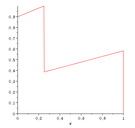
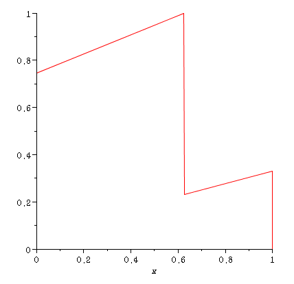
Figure 5: Graphs of $g$ for $a=0.3$ and $0.6$ (left, right)

4 Discussions

4.1 The Triangular Transition

In this subsection, we will first discuss the behavior of the map $T$ when $\lambda$ is close to $0.8$ near the singular line $\overleftrightarrow{AB}$, and state the results of previous section for more general parameters.

The outer billiards map, either with or without contraction, is invariant under affine transformations of the plane. That is, if a convex polygon $P$ is mapped to another polygon $Q$ by an orientation-preserving affine map, the dynamics of $T$ (either with or without contraction) outside $P$ and $Q$ are conjugated by a linear map. Up to affine transformations, any convex quadrilateral is represented by a pair of reals $(a,b)$ where $0<a$, $b<1$, and $ab<1$. This pair represents the quadrilateral with vertices $A=(0,1)$, $B=(a,1)$, $C=(1,b)$, and $D=(0,0)$. Moreover, we can cyclically rename the vertices; the permutation $(A,B,C,D)$$\rightarrow$$(D,A,B,C)$ correspond to the transformation $(a,b)\mapsto(1-b,(1-1/a)/(1-b))$ and one can easily check from this that we can further assume $0<a<1$ and $0<b<1$ without loss of generality.

Let us say that a periodic orbit is triangular if its period is 3. If we consider quadrilaterals satisfying $a+b\leq 1$, then two triangular periodic orbits exist in disjoint ranges of $\lambda$. It can be proved by a simple computation. Furthermore, let us say that a periodic orbit is regular if every point lies on the set $X$. Otherwise, a periodic orbit will be called degenerate. While a regular periodic orbit is necessarily locally attracting, a degenerate periodic orbit of odd period is never locally attracting.

Proposition 4.1.

If $a+b\leq 1$, the quadrilateral $(a,b)$ has the regular triangular periodic orbit skipping the vertex $A$ (resp. vertex $B$) precisely in the range $a<\lambda<1-b$ (resp. $1-b<\lambda<1$).

That is, at the critical value $\lambda=1-b$, two triangular periodic orbits both exist but in degenerate forms; each periodic orbit has two points on the line $\overleftrightarrow{AB}$. Also, we note that in the range $\lambda\in(a,1)\backslash\{1-b\}$, some neighborhood of the singular ray extending $\overline{AB}$ is attracted to the triangular periodic orbit. However, when $\lambda=1-b$, both of them are not attracting (since the period is odd), so it is believable that a new attractor should appear to compensate for this loss. We have seen in Corollary 3.1 and Theorem 2 that such a new attractor is either a degenerate periodic orbit of high period or a Cantor set.

To illustrate this by an example, let us consider the quadrilateral $P=(0.5,0.2)$. In this specific case, in the range $a=0.5<\lambda<0.8=1-b$, the whole domain is asymptotic to the triangular orbit skipping $A$ (left one in Figure 6), while in the range $0.8<\lambda<0.85$, the whole domain is attracted to the triangular orbit skipping $B$. (right one in Figure 6) At the critical value $\lambda=0.8$, a degenerate periodic orbit of period 10 (one of the ten points lies near the midpoint of the edge $\overline{AB}$) suddenly appears and attracts the whole domain. In general for different quadrilaterals, a few other periodic orbits can simultaneously exist near the bifurcation value $\lambda=1-b$ but the ones that exist for values of $\lambda$ smaller than $1-b$ are qualitatively different from the ones that exist for $\lambda$ greater than $1-b$. See [12] for more explanations and pictures regarding this issue.

We state the most general parameter range in which considerations from the previous section apply without any extra effort.

Theorem 3.

Let $(a,b)$ satisfy $0<a,b<1$, $a+b\leq 1$, $a<1+\lambda-\lambda^{3}-\lambda^{4}$. Then with $P=(a,b)$ and $\lambda=1-b$, $g$ is likewise well-defined piecewise contraction given by the formula 2 whose rotation number is well-defined, and when $\rho(g)$ is rational, at most two periodic orbits exist and every point in $X\cap(R_{1}\cup R_{2})$ is asymptotic to one of them, and when $\rho(g)$ is irrational, every point in $X\cap(R_{1}\cup R_{2})$ is asymptotic to a unique Cantor set.

We show in Figure 7 how the rotation number $\rho(g)$ varies in the parameter plane $0<a,b<1$, $a+b\leq 1$, $a<1+\lambda-\lambda^{3}-\lambda^{4}$. Without the inequality $a<1+\lambda-\lambda^{3}-\lambda^{4}$ (which guarantees $T^{3}R_{1}\subset R_{2}$ among other things), the dynamics is quite different and more complicated. The central “band” corresponds to $\rho=0.5$, and the large upper and lower regions correspond to $\rho=0$. If we fix $b\in(0,0.5)$ and then the graph of the function $a\mapsto\rho(g_{a,b})$ (where $g_{a,b}$ is the map $g$ with the polygon $P=(a,b)$) is a devil’s staircase.

Next, let us take a look at cases where the rotation numbers are rational. In Figure 8, the bifurcation attracting periodic orbits are drawn for $P=(a,b=0.15)$ where $a=$0.30, 0.33, 0.34, 0.35, 0.40, 0.50 in clockwise order starting from the top left picture. They correspond to rotation numbers 1, 6/7, 4/5, 3/4, 2/3, 1/2, respectively. One can easily see that the period increases in proportion to the denominator of the rotation number.

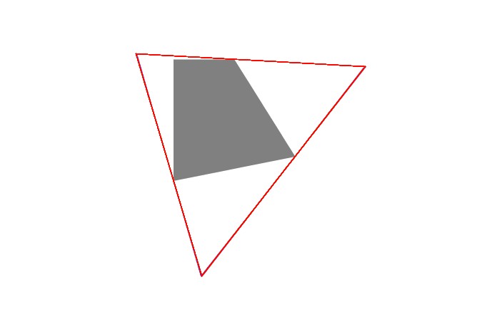
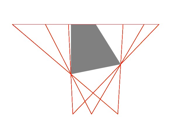
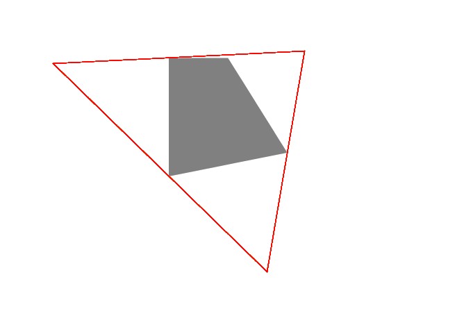
Figure 6: Attracting periodic orbits for $P=(0.5,0.2)$ when $\lambda=0.75,0.8,0.85$ (from left to right)

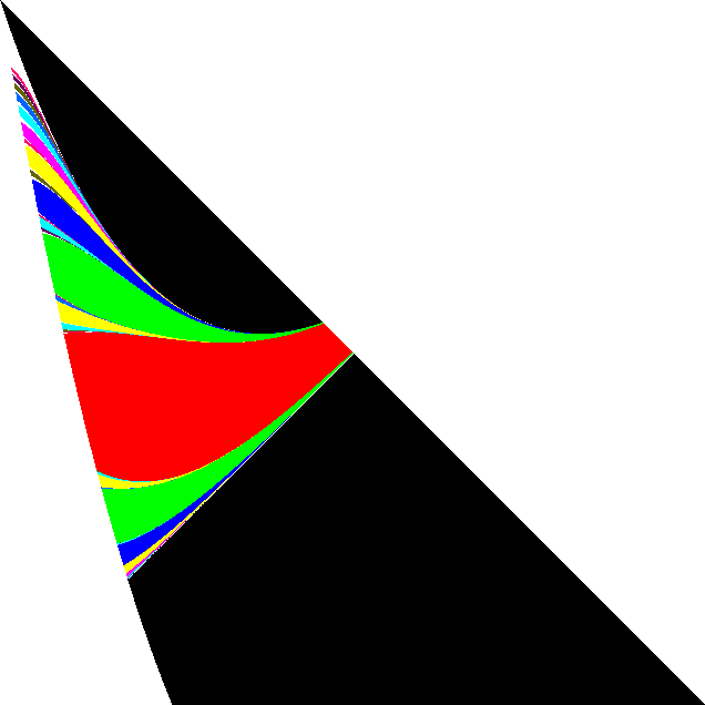
Figure 7: Rotation number $\rho(g)$ as a function of $a$ and $b$; the top left corner is $a=b=0$, and the horizontal axis is $b$.

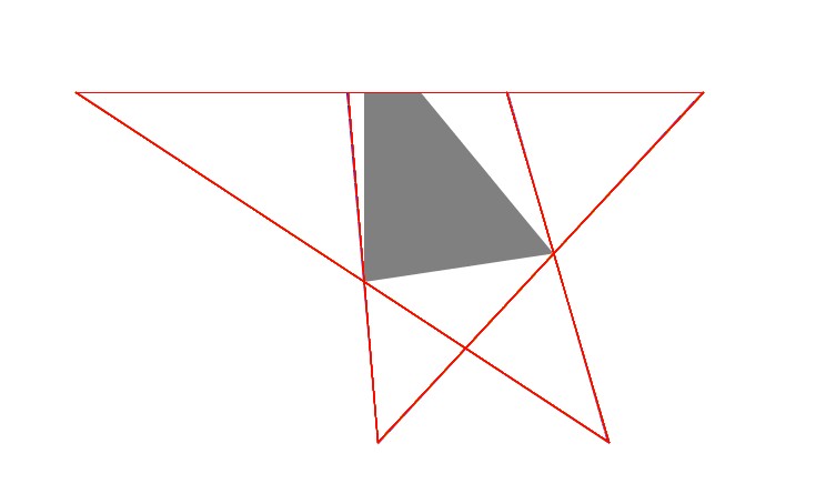
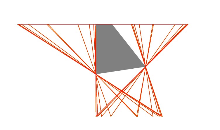
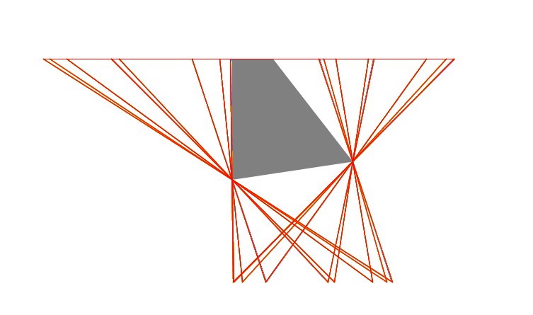
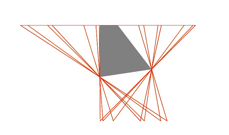
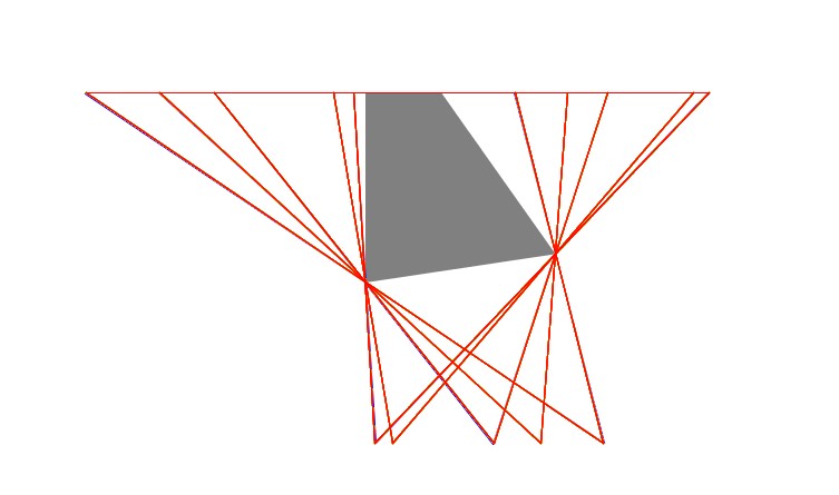
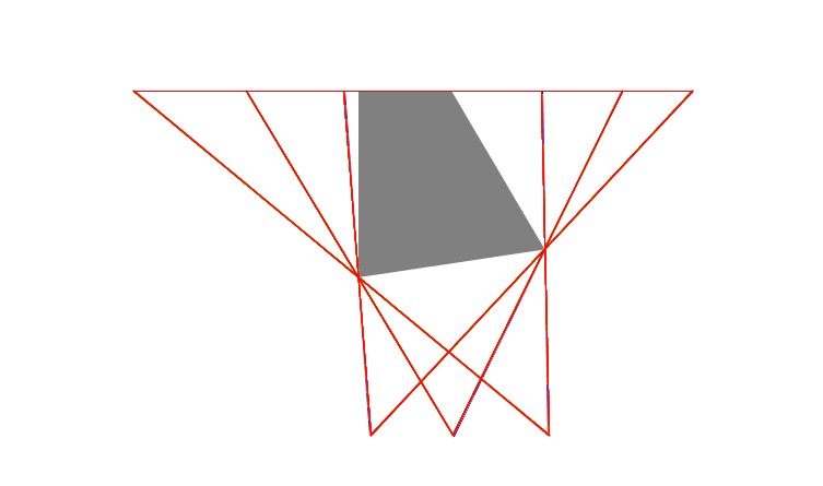
Figure 8: Attracting periodic orbits for various rational rotation numbers

4.2 Global Uniqueness and Unique Ergodicity

One might suspect that the set of points in $\mathbb{R}^{2}\backslash P$ that are asymptotic to the attractor constructed above is rather small. Indeed, experiment suggests that for most pairs of $(a,b)$ considered in the previous subsection, every regular point $p\in\mathbb{R}^{2}\backslash P$ has a forward iterate in $R_{1}\cup R_{2}$. Or equivalently, the inverse iterates of $R_{1}\cup R_{2}$ covers the whole domain $\mathbb{R}^{2}\backslash P$. While this seems to hold in particular for the 1-parameter family of quadrilaterals considered the previous section, we will only prove this statement for the parameters $0.4\leq a\leq 0.5$ and $b=0.4$ (hence $\lambda=0.6$). Later it will become clear why this statement is easier to verify for small $\lambda$.

For each pair $(a,b)$, we denote the unique attractor for points in $X\cap(R_{1}\cup R_{2})$ by $K_{(a,b)}$.

Theorem 4.

In the parameter range $0.4\leq a\leq 0.5$ and $b=0.4$ ($\lambda=0.6$), the entire domain is asymptotic to $K_{(a,b)}$. In particular, there exists values of $(a,b)$ for which the entire domain is asymptotic to a single Cantor set.

Proof.

We first note that when $a=0.4$, $\rho(g)=0$ and when $a=0.5$, $\rho(g)=1/3$. Hence, there exist values of $a$ between $0.4\leq a\leq 0.5$ such that $\rho(g)$ is irrational. Now the proof consists of showing three statements:

1. First, we construct a forward-invariant ball $\mathcal{B}$ such that every point in $\mathbb{R}^{2}\backslash P$ has a forward iterate in $\mathcal{B}$.

2. Then we construct a pentagonal region $Z_{0}$ which for all $\epsilon>0$ (thickness of the rectangles $R_{1}$ and $R_{2}$) satisfies $T^{N(\epsilon)}Z_{0}\subset R_{1}\cup R_{2}$ for some large $N(\epsilon)>0$.

3. Finally, we show that $\mathcal{B}\subset Z_{0}\cup T^{-1}Z_{0}\cup T^{-2}Z_{0}\cup T^{-3}Z_{0}$.

Then from 1, 2, and 3, we are done; any point in $\mathbb{R}^{2}\backslash P$ has a forward iterate in $\mathcal{B}$ (by 1), and then it has a forward iterate in $Z_{0}$ (by 3), which has a forward iterate in $R_{1}\cup R_{2}$ (by 2). These statement will be proved in Lemmas 4.1, 4.2, and 4.3, respectively.∎

Lemma 4.1.

Take $\epsilon^{\prime}>0$ arbitrary. Consider the max metric on the plane: $||(x,y)||=\max\{|x|,|y|\}$ and we define $\mathcal{B}$ be the ball of radius $2+\epsilon^{\prime}$ in this metric with center $(0.5,0.5)$. Then for $0.4\leq a\leq 0.5$ and $b=0.4$, it is forward-invariant and every point in $\mathbb{R}^{2}\backslash P$ has a forward iterate in $\mathcal{B}$.

Proof.

This follows from a general fact; let $||\cdot||$ be any norm on the plane, and let $\{v_{1},...,v_{n}\}$ be the set of vertices of $P$. Then for a point $w\in\mathbb{R}^{2}\backslash P$, let us assume that

$$||w||=\frac{1+\lambda}{1-\lambda}\max_{i}||v_{i}||+\delta$$

where $\delta>0$. Since $Tw=(1+\lambda)v-\lambda w$ for some vertex $v$ of $P$, we have

$$||Tw||\leq(1+\lambda)\max||v_{i}||+\lambda\frac{1+\lambda}{1-\lambda}\max||v_{i}||+\lambda\delta=\frac{1+\lambda}{1-\lambda}\max_{i}||v_{i}||+\lambda\delta$$

and hence

$$\limsup_{n\rightarrow\infty}||T^{n}w||\leq\frac{1+\lambda}{1-\lambda}\max_{i}||v_{i}||.$$

Moreover, when we have

$$||w||\leq\frac{1+\lambda}{1-\lambda}\max_{i}||v_{i}||,$$

we deduce

$$||Tw||\leq\frac{1+\lambda}{1-\lambda}\max_{i}||v_{i}||.$$

Now, in our circumstances we have $\lambda=0.6$ and $||v_{i}||=0.5$ for all $i$, with respect to the center $(0.5,0.5)$. Hence any ball of radius strictly greater than $2$ centered at $(0.5,0.5)$ will do the job. ∎

We will now present the region $Z_{0}$. For this, it is necessary to construct some extra points: (see Figure 10)

• $D^{1}=(0,\frac{8}{3})$: the point on $\overrightarrow{DA}$ such that $|D^{1}A|:|AD|=1/\lambda$.

• $C^{1}=(-\frac{5}{3},-\frac{2}{3})$: the point on $\overrightarrow{CD}$ such that $|C^{1}D|:|DC|=1/\lambda$.

• $D^{2}=(\frac{8}{3},-\frac{152}{45})$: the point on $\overrightarrow{D^{1}C}$ such that $|D^{2}C|:|CD^{1}|=1/\lambda$.

• $L=(\frac{8}{3},-\frac{2a+3}{5(1-a)})$: the intersection of $\overleftrightarrow{BC}$ with the vertical line through $D^{2}$.

• $L^{1}=(-\frac{40}{9},\frac{2a+3}{3(1-a)})$: the point on $\overrightarrow{LD}$ such that $|L^{1}D|:|DL|=1/\lambda$.

• $C^{2}=(\frac{25}{9},\frac{34}{9})$: the point on $\overrightarrow{C^{1}A}$ such that $|C^{2}A|:|AC^{1}|=1/\lambda$.

• $E=(\frac{5}{9}(8-5a),1)$: the intersection of the line $\overleftrightarrow{AB}$ with the line $\overleftrightarrow{L^{1}C^{1}}$.

• $E^{1}=(\frac{25}{27}(8-5a),1)$: the point on $\overrightarrow{EA}$ such that $|E^{1}A|:|AE|=1/\lambda$.

• $M=(\frac{5}{9}\frac{34a-49}{2a-5},\frac{2}{9}\frac{34a-49}{2a-5})$: the intersection of $\overleftrightarrow{C^{2}J^{1}}$ with $\overleftrightarrow{CD}$.

• $M^{1}=(-\frac{25}{27}\frac{34a-49}{2a-5}+\frac{8}{3},-\frac{10}{27}\frac{34a-49}{2a-5}+\frac{16}{15})$: the point on $\overrightarrow{MC}$ such that $|M^{1}C|:|CM|=1/\lambda$.

• $A^{1}=(\frac{8a}{3},1)$: the point on $\overrightarrow{AB}$ such that $|A^{1}B|:|BA|=1/\lambda$. Here it is important that the $x$-coordinate of $A^{1}$ is greater than the $x$-coordinate of $C$.

• $A^{2}=(-\frac{40a}{9}+\frac{8}{3},-\frac{3}{5})$: the point on $\overrightarrow{A^{1}C}$ such that $|A^{2}C|:|CA^{1}|=1/\lambda$.

We have four extra points whose coordinates will not be important.

• $N_{1}$: the intersection of the vertical line through $A^{1}$ with the line $BC$.

• $N_{2}$: the intersection of the vertical line through $A^{2}$ with the line $DC$.

• $N_{3}$: the intersection of the horizontal line through $A^{2}$ with the line $DC$.

• $N_{4}$: the intersection of the horizontal line through $D^{1}$ with the vertical line through $L^{1}$.

Now we are ready to define the region $Z_{0}$ as well as other regions $Z_{1},...,Z_{6}$. We orient the vertices in clockwise order. Again, see Figure 10.

• $Z_{0}$: this is the pentagon with vertices $L^{1},N_{4},D^{1},D$, and $C^{1}$. For this to be well-defined, we check that the $y$-coordinate of $D^{1}$ is greater than or equal to the $y$-coordinate of $L^{1}$ in the range $a\in[0.4,0.5]$. Indeed, for $a=0.5$, points $N_{4}$ and $L^{1}$ coincides and $Z_{0}$ becomes a quadrilateral.

• $Z_{1}$: this is the quadrilateral with vertices $D^{1},C^{2},E^{1}$, and $A$.

• $Z_{2}$: this is the quadrilateral with vertices $A^{1},E^{1},L$, and $N_{1}$.

• $Z_{3}$: this is the triangle with vertices $B,A^{1}$, and $N_{1}$.

• $Z_{4}$: this is the right-angle triangle with vertices $N_{2},A^{2},$ and $N_{3}$.

• $Z_{5}:$ this is the pentagon with vertices $N_{3},G,L,D^{2},$ and $M^{1}$.

• $Z_{6}$: this is the quadrilateral with vertices $N_{2},C,G,$ and $A^{2}$.

Lemma 4.2.

For all $\epsilon>0$, there exists large $N>0$ such that $T^{N}Z_{0}\subset R_{1}\cup R_{2}$ where $\epsilon$ is the thickness of rectangles $R_{1}$ and $R_{2}$.

Proof.

The segment $\overline{EA}$ divides $Z_{0}$ to two regions; denote them by $Z_{0}^{+}$ (one above) and $Z_{0}^{-}$ (one below). Note that these regions contain the segment $\overline{EA}$, which is the domain of our first-return maps $f$ and $g$ analyzed in the previous section. Therefore, it is enough to prove that $Z_{0}$ is forward-invariant and that points in $Z_{0}$ converge to the line segment $\overline{EA}$ under the iteration of the first-return map to $Z_{0}$. This proof is parallel to the proof of Lemma 3.1 and we will only sketch it. See Figure 9.

Consider the rectangle which has three vertices $N_{4},D^{1},$ and $A$. This rectangle contains $Z_{0}^{+}$. Then it is elementary to check that $T^{3}$ of this rectangle is again a rectangle contained in $Z_{0}^{-}$ with one vertex $A$. The $y$-coordinates of points in $Z_{0}^{+}$ relative to $1$ (the $y$-coordinate of the line $AB$) have contracted by $\lambda^{3}$ in $T^{3}(Z_{0}^{+})$.

Next, note that $T^{3}(Z_{0}^{-})$ naturally splits into two regions, say $Z^{\prime}$ (the one on the left) and $Z^{\prime\prime}$ (the one on the right), by the vertical line $AD$. First, $Z^{\prime}$ is contained in $Z_{0}^{+}$ so we are good. Next, $T(Z^{\prime\prime})$ is contained in $Z_{0}^{-}$ and we note that the $y$-coordinates of the points in $T(Z^{\prime\prime})$ relative to $1$ have contracted by $\lambda^{4}$. We are done. ∎

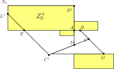
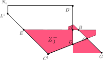
Figure 9: Left: $T^{3}Z_{0}^{+}\subset Z_{0}^{-}$, right: $T^{3}Z_{0}^{-}=Z^{\prime}\cup Z^{\prime\prime}$ where $Z^{\prime}\subset Z_{0}^{+}$ and $T(Z^{\prime\prime})\subset Z_{0}^{-}$. (drawn for $a=0.4$)

The following is the most tedious lemma to prove. It will be much harder to prove for larger values of $\lambda$.

Lemma 4.3.

$\mathcal{B}\subset Z_{0}\cup T^{-1}Z_{0}\cup T^{-2}Z_{0}\cup T^{-3}Z_{0}$.

Proof.

We prove $\mathcal{B}\subset\cup_{i=0}^{6}Z_{i}$ and $\cup_{i=0}^{6}Z_{i}\subset Z_{0}\cup T^{-1}Z_{0}\cup T^{-2}Z_{0}\cup T^{-3}Z_{0}$.

For the first statement, it is enough to check the following for all $a\in[0.4,0.5]$, each of which is a simple computation using the expression for coordinates given above:

• the $x$-coordinate of $C^{1}$ is strictly less than $-1.5$.

• the $y$-coordinates of $M^{1}$ and $D^{2}$ are both strictly less than $-1.5$.

• the $x$-coordinate of $L$ is strictly greater than $2.5$.

• the $y$-coordinate of $D^{1}$ is strictly greater than $2.5$.

• finally, the point $(2.5,2.5)$ (upper right corner) lies below the line $C^{2}E^{1}$.

In Figure 10, the ball of radius $2$ is drawn for the case $a=0.4$.

The second statement is reduced to check all of the following:

• $T(Z_{1})=Z_{0}^{-}$: this is simply how $Z_{1}$ is defined.

• $T(Z_{2})\subset Z_{0}^{+}$: enough to check that the vertex $L$, after reflecting on $B$, gets inside $Z_{0}^{+}$.

• $T^{2}(Z_{3})\subset Z_{0}^{-}$: this is straightforward.

• $T(Z_{4})\subset Z_{2}$: enough to check that the vertex $N_{3}$, after reflecting on $C$, gets inside the segment $\overline{A^{1}E^{1}}.$ Hence $T^{2}(Z_{4})\subset Z_{0}$.

• $T(Z_{5})\subset Z_{1}$: this follows from the definition of $Z_{5}$. Hence $T^{2}(Z_{5})\subset Z_{0}$.

• $T(Z_{6})\subset Z_{3}$: this is simply how $Z_{6}$ is defined. Hence $T^{3}(Z_{6})\subset Z_{0}$.

We are done. ∎

For each pair $(a,b)$ satisfying $0<a,b<1$, $a+b\leq 1$, $a<1+\lambda-\lambda^{3}-\lambda^{4}$ $(\lambda=1-b$), recall that we had a unique attractor $K_{(a,b)}$ for points in $X\cap(R_{1}\cup R_{2})$. Then we have the following result.

Theorem 5.

For each $(a,b)$, there is a unique Borel $T$-invariant probability measure $\mu_{(a,b)}$ supported on the set $K_{(a,b)}$, such that for each continuous function $\phi$ on $\mathbb{R}^{2}\backslash P$,

$$\lim_{n\rightarrow\infty}\frac{\sum_{i=0}^{n-1}\phi(T^{i}x)}{n}\rightarrow\int\phi|_{K_{(a,b)}}d\mu_{(a,b)}$$

holds for all $x\in X\cap(R_{1}\cup R_{2})$, and for all $x\in X$ for parameters in the range $a\in[0.4,0.5]$, $b=0.4$.

Proof.

We first prove that $g$ is uniquely ergodic (that is, $g$ has only one Borel invariant probability measure supported on the common $\omega$-limit set of its regular points). In the case when $\rho(g)$ is rational, every orbit is asymptotic to a single periodic orbit and hence the atomic probability measure supported on this periodic orbit is the unique invariant measure. When $\rho(g)$ is irrational, we repeat the unique ergodicity argument for the circle homeomorphism (with irrational rotation number) explained in detail in [13]. One can still construct a semiconjugacy between $g$ and the irrational rotation by angle $\rho(g)$.

In the same way, $f$ is uniquely ergodic as well, and we obtain an invariant probability measure of $T$ by a linear combination of invariant measures for $f$ and $g$ (viewed as measures on the segment $\overline{EA}$) and their pushforwards by $T$. Moreover, given an invariant measure for $T$ supported on $K_{a}$, we obtain invariant measures for $f$ and $g$. Therefore, $T$ is uniquely ergodic on the union of $X\cap(R_{1}\cup R_{2})$ and its forward iterates.

Now the statement regarding the Birkhoff average holds for $f$ and $g$ and therefore it holds for $T$ as well. ∎

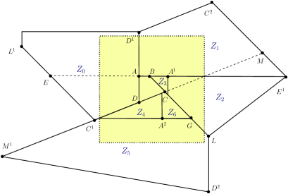
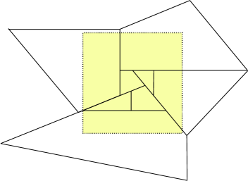
Figure 10: Extra points and regions, drawn for $a=0.4$ (above) and $a=0.5$ (below)

References

- [1] Rafael A. Rosales Arnaldo Nogueira, Benito Pires. Asymptotically periodic piecewise contractions of the interval. arXiv:1206.5676, 2013.
- [2] Romain Brette. Rotation numbers of discontinuous orientation-preserving circle maps. Set-Valued Analysis, Volume 11, Number 4:359–371, 2003.
- [3] Henk Bruin and Jonathan H. B. Deane. Piecewise contractions are asymptotically periodic. Proc. Amer. Math. Soc., 137(4):1389–1395, 2009.
- [4] Eleonora Catsigeras, Álvaro Rovella, and Ruben Budelli. Contractive piecewise continuous maps modeling networks of inhibitory neurons. Int. J. Pure Appl. Math., 61(4):381–407, 2010.
- [5] Christopher Chase, Joseph Serrano, and Peter J. Ramadge. Periodicity and chaos from switched flow systems: contrasting examples of discretely controlled continuous systems. IEEE Trans. Automat. Control, 38(1):70–83, 1993.
- [6] Leon O. Chua and Tao Lin. Chaos in digital filters. IEEE Trans. Circuits and Systems, 35(6):648–658, 1988.
- [7] Jonathan H. B. Deane. Piecewise isometries: applications in engineering. Meccanica, 41(3):241–252, 2006.
- [8] Eugene Gutkin Gianluigi Del Magno, Jos Pedro Gaivao. Dissipative outer billiards: a case study. arXiv:1310.4724, 2013.
- [9] Pedro Duarte Jos Pedro Gaiv o Diogo Pinheiro Gianluigi Del Magno, Jo o Lopes Dias. Chaos in the square billiard with a modified reflection law. arxiv.org/pdf/1112.1753, 2012.
- [10] Pedro Duarte Jos Pedro Gaiv o Diogo Pinheiro Gianluigi Del Magno, Jo o Lopes Dias. Srb measures for hyperbolic polygonal billiards. arXiv:1302.1462, 2013.
- [11] Eugene Gutkin and Nándor Simányi. Dual polygonal billiards and necklace dynamics. Comm. Math. Phys., 143(3):431–449, 1992.
- [12] In-Jee Jeong. Outer billiards with contraction. Senior Thesis, Brown University, 2013.
- [13] A. Katok and B. Hasselblatt. Introduction to the Modern Theory of Dynamical Systems. Cambridge Univ. Press, Cambridge, 1995.
- [14] Julien Cassaigne Nicolas Bedaride. Outer billiard outside regular polygons. J. London Math. Soc., 2011.
- [15] Arnaldo Nogueira and Benito Pires. Dynamics of piecewise contractions of the interval. arXiv:1206.5676, 2012.
- [16] Frank Rhodes and Christopher L. Thompson. Rotation numbers for monotone functions on the circle. J. London Math. Soc. (2), 34(2):360–368, 1986.
- [17] Frank Rhodes and Christopher L. Thompson. Topologies and rotation numbers for families of monotone functions on the circle. J. London Math. Soc. (2), 43(1):156–170, 1991.
- [18] Richard Evan Schwartz. Unbounded orbits for outer billiards. I. J. Mod. Dyn., 1(3):371–424, 2007.
- [19] Richard Evan Schwartz. Outer billiards on kites, volume 171 of Annals of Mathematics Studies. Princeton University Press, Princeton, NJ, 2009.
- [20] Richard Evan Schwartz. Outer billiards, arithmetic graphs, and the octagon. arXiv:1006.2782, 2010.
- [21] Richard Evan Schwartz. Outer billiards on the Penrose kite: compactification and renormalization. J. Mod. Dyn., 5(3):473–581, 2011.
- [22] S. Tabachnikov. On the dual billiard problem. Adv. Math., 115(2):221–249, 1995.
- [23] Serge Tabachnikov. Billiards. Panor. Synth., (1):vi+142, 1995.