Contact Manifolds in a Hyperbolic System
of Two Nonlinear Conservation Laws

Abstract

This paper deals with a hyperbolic system of two nonlinear conservation laws, where the phase space contains two contact manifolds. The governing equations are modelling bidisperse suspensions, which consist of two types of small particles that are dispersed in a viscous fluid and differ in size and viscosity. For certain parameter choices quasi-umbilic points and a contact manifold in the interior of the phase space are detected. The dependance of the solutions structure on this contact manifold is examined. The elementary waves that start in the origin of the phase space are classified. Prototypic Riemann problems that connect the origin to any point in the state space and that connect any state in the state space to the maximum line are solved semi-analytically.

1 Introduction

Polydisperse suspensions can be described by balance equations as $N$ superimposed continuous phases, where particles of species $i$, associated with a volume fraction $\phi_{i}$, distinguish in properties like size, density and viscosity [7, 12]; models with similar solution structure describe traffic and pedestrian flows [4, 8]. For the considered model of bidisperse suspension, the solution structure of the solution to the initial value problem for standard batch settling tests has been studied for the cases when strict hyperbolicity is assured [5] and when the phase space provides elliptic regions [6]. The focus of this contribution is on the impact of a contact manifold in the interior of the phase space, that emerges for certain parameter settings. This contact manifold has the physical property of coinciding particle settling velocities, and thus has a practical relevance, since one general goal in the process control of solid-liquid separation processes is to reduce segregation effects [10].

The generic form of kinematic sedimentation models for polydisperse suspensions consists of the system of $N$ first-order hyperbolic equations

$$\partial_{t}\phi_{i}+\partial_{x}f_{i}(\Phi)=0,\quad f_{i}(\Phi)=\phi_{i}v_{i}(\Phi),\quad i=1,\dots,N,$$ (1)

where $t$ is time, $x$ is depth and the velocity components $v_{i}(\Phi)$ depend on the concentration vector $\Phi=(\phi_{1},\dots,\phi_{N})^{\mathrm{T}}$. The unknown $\Phi$ denotes the vector of volume fractions of the solids phases and is contained by the phase space of physically relevant concentrations

$$\mathcal{D}_{\Phi^{\infty}}:=\bigg{\{}\Phi=(\phi_{1},\dots,\phi_{N})^{\mathrm{T}}\in\mathbb{R}^{N}:\begin{array}[]{l}\phi_{1}\geq 0,\ldots,\,\phi_{N}\geq 0,\\ \phi:=\phi_{1}+\ldots+\phi_{N}\leq\phi^{\infty}\end{array}\bigg{\}},$$ (4)

where the total concentration $\phi:=\phi_{1}+\ldots+\phi_{N}$ is bounded from above by the maximum packing concentration $\phi^{\infty}$. The maximum packing manifold

$$\partial^{\infty}:=\{\Phi=(\phi_{1},\dots,\phi_{N})^{\mathrm{T}}:\phi:=\phi_{1}+\dots+\phi_{N}=\phi^{\infty}\}.$$ (5)

is the set of all maximal states.

The resulting system of conservation laws is actually a system of mass balances for different solids species, where the nonlinear flux function

$$\boldsymbol{f}(\Phi):=(f_{1}(\Phi),\dots,f_{N}(\Phi))^{\mathrm{T}}$$

can be derived from the corresponding momentum balances [7, 12, 24] The components describe the flow process of the dispersed solids phases in a liquid, where the dispersed phases are considered as a continuum. The flux function has components

$$f_{i}(\Phi)=\phi_{i}v_{i}(\Phi),\qquad v_{i}(\Phi)=u_{i}(\Phi)-\Phi^{\mathrm{T}}\mbox{{\boldmath$u$}},\;\quad i=1,\dots,N,$$ (6)

with $\mbox{{\boldmath$u$}}=(u_{1}(\Phi),\dots,u_{N}(\Phi))^{\mathrm{T}}$, where the absolute velocity $v_{i}=v_{i}(\Phi)$ of a representative solids particle depends on a linear combination of the solid-fluid relative (“slip”) velocities

$$u_{i}(\Phi):=v_{i}(\Phi)-v_{\mathrm{f}},$$ (7)

which are relative to the fluid velocity $v_{\mathrm{f}}$. The flux function model (6) is closed by specifying the relative velocity as

$$u_{i}(\Phi)=v_{\infty i}V_{i}(\Phi),$$ (8)

where the constant $v_{\infty i}$ is the Stokes velocity, which quantifies the settling velocity of a single particle in a fluid, and $V_{i}(\Phi)$ is the hindered-settling velocity that is an non-increasing function of the components of $\Phi$, see [3]. Following Richardson and Zaki [28], the hindered-settling velocity is set as

$$V_{i}(\Phi):=\begin{cases}(1-\phi)^{n_{i}-1}&\text{if $0\leq\phi\leq\phi^{\infty}$,}\\ 0&\text{otherwise,}\end{cases}\quad i=1,\dots,N,$$ (9)

where the exponent $n_{i}>1$ accounts for the slow down of the process at increasing concentrations. Assumptions (8) and (9) can be combined as

$$u_{i}(\Phi)=v_{\infty i}(1-\phi)^{n_{i}-1}$$ (10)

for $\Phi\in\mathcal{D}_{\Phi^{\infty}}$.

Strictly hyperbolic systems of conservation laws, where the eigenvalues of the Jacobian matrix of the flux function are real and distinct, provide a relatively well understood framework for the solution of Riemann problems [15]. In [12], strict hyperbolicity of the system (1) with flux function (6) has been first shown for $N=2$ and later on in [7] for general $N$, but up to then only for coinciding hindered-settling factors $V_{1}(\phi)=V_{2}(\phi)=\dots=V_{N}(\phi)$, which depend on the total concentration $\phi$. For a model with the more general hindrance factor (9), this implies to have constant exponents $n_{1}=n_{2}=\dots=n_{N}$, a restriction that turned out to be unnecessary: In [3], it is shown that strict hyperbolicity also holds for general $N\geq 2$ and relative velocities of form $V_{i}(\Phi)=V_{i}(\phi)$ as long as the inequality

$$u_{i}^{\prime}(1-\phi)-u_{i}<0$$ (11)

holds for all $i=1,\dots,N$, where $u_{i}^{\prime}$ denotes the derivative with respect to $\phi$; in this situation the only restriction on the hindered-settling function $V_{i}(\Phi)=V_{i}(\phi)$ is to depend on the total concentration $\phi$. The inequality (11) is satisfied in particular when the relative velocities are ordered as $u_{1}>u_{2}>\dots>u_{n}$ for any $\phi$. This holds in the case of the hindered-settling function (9) for the situation if the parameters are ordered as

$$v_{\infty 1}>v_{\infty 2}>\dots>v_{\infty N}\quad\text{with}\quad n_{1}<n_{2}<\dots<n_{N}.$$ (12)

In [17], a secular equation framework was established that allows to verify strict hyperbolicity by checking a simple algebraic criterion; this framework has been applied to the considered model with a Richardson-Zaki hindered settling function having constant exponent. In [9], this framework was adapted to the same general model setting as in [3], i.e. with size-dependent hindered settling factors that not necessarily take the form (9). Subsequently, in [11] the secular equation framework was applied to a series of choices of hindered-settling functions.

Preliminary numerical simulations of Riemann problems for $N=3$ with arbitrary parameter choices (not exposed here) showed that strict hyperbolicity might fail as coincidence of eigenvalues occurs, providing an abrupt change of the solution structure. The fact that this phenomenon of abrupt change already appears for $N=2$ made us to look for analytical insights in this situation, which lead to the present contribution.

This contribution deals with the wave classification for $2\times 2$ systems of conservation laws that arise as one-dimensional kinematic models for the sedimentation of bidisperse suspensions. The analytical examination of bidisperse suspensions gives insights to flow properties of polydisperse suspensions, which are mixtures of small solid particles dispersed in a viscous fluid. In this contribution the focus is on models for particle suspension where all particles are assumed to have the same density. Specifically, in this contribution, the properties of the $2\times 2$ system (1) (with $N=2$), flux function (6) and closures (8), (9) are studied. The model of our interest contemplates the following specifications, which is done in opposition to (12), which would guarantee strict hyperbolicity:

(S1) $v_{\infty 1}\,\,\,>\,\,\,v_{\infty 2}\,\,\,>\,\,\,0$,

(S2) $n_{1}\,\,\,>\,\,\,n_{2}\,\,\,>\,\,\,1$,

(S3) $\phi^{\infty}\,\,\equiv\,\,1$.

For $N=2$ and $V_{i}(\phi)$ given by (9) the flux function $\boldsymbol{f}(\Phi)=(f_{1}(\Phi),f_{2}(\Phi))^{\mathrm{T}}$ takes the form

$$f_{1}(\Phi)=\phi_{1}\Bigl{(}v_{\infty 1}(1-\phi_{1})(1-\phi)^{n_{1}-1}-v_{\infty 2}\phi_{2}(1-\phi)^{n_{2}-1}\Bigr{)},$$

$$f_{2}(\Phi)=\phi_{2}\Bigl{(}v_{\infty 2}(1-\phi_{2})(1-\phi)^{n_{2}-1}-v_{\infty 1}\phi_{1}(1-\phi)^{n_{1}-1}\Bigr{)},$$

for values $\Phi\in\mathcal{D}_{\Phi^{\infty}}$ and $f_{1}(\Phi)=f_{2}(\Phi)=0$ otherwise. A special interest consists in the classification of the solution structure of the Riemann problem

$$\Phi(t=0,x)=\begin{cases}\Phi^{-}\quad\text{if}\quad x<0,\\ \Phi^{+}\quad\text{if}\quad x>0.\end{cases}$$ (13)

For convenience, the Riemann problem consisting of the system of PDEs (1) with initial condition (13) is referred to as $\mathrm{RP}(\Phi^{-},\Phi^{+})$, with left and right values $\Phi^{-}$ and $\Phi^{+}$, respectively, to be specified.

The application of this model is the batch settling process of an initially homogeneous suspension in a closed container described by the initial-boundary value problem

$$\partial_{t}\phi_{i}+\partial_{x}f_{i}(\Phi)=0,\quad i=1,2,$$

$$\Phi(0,x)=\Phi_{0}(x),\quad 0\leq x\leq L,$$ (14)

$$f_{i}(\Phi)=0,\quad x\in\{0,L\},\quad i=1,2,$$ (15)

where $L$ is the domain height and the components of the flux-density vector $\boldsymbol{f}(\Phi)=(\smash{f_{1}}(\Phi),\smash{f_{2}}(\Phi))^{\mathrm{T}}$ are given by (6). Because of the zero-flux boundary condition (15), the initial-boundary data (14) and (15) can be replaced by the Cauchy data

$$\Phi(0,x)=\Phi_{0}(x)=\begin{cases}O&\text{for $x<0$,}\\ \Phi_{0}&\text{for $0\leq x\leq L$,}\\ \Phi^{\infty}&\text{for $x>L$,}\end{cases}$$ (16)

where $O:=(0,\,0)^{\mathrm{T}}$ is the origin and $\Phi^{\infty}$ is a state on the maximum concentration manifold (5). Therefore, the Riemann problems $\mathrm{RP}(O,\Phi)$ and $\mathrm{RP}(\Phi,\Phi^{\infty})$ are of particular interest. This contribution reveals analytical insights into the solution structure of the Riemann problem $\mathrm{RP}(O,\Phi)$. From an application point of view, the Riemann problem $\mathrm{RP}(O,\Phi)$ describes the interactions on the upper interface between clear liquid and initially homogeneous suspension during a batch settling process.

With respect to related work, several studies on weakly hyperbolic systems, i.e. systems that are hyperbolic but not strictly hyperbolic, are developed for models of multi-phase flow in porous media. For three-phase flow in porous media, the Corey model with convex permeability leads to a single isolated point, the so-called umbilic point, in which strict hyperbolicity fails [13, 20, 21, 25, 29]; another loss of hyperbolicity occurs when a the phase space contains an elliptic region as it occurs for the Stone model [18]. To solve Riemann problems, the wave-curve method has been applied, in which a sequence of elementary waves are connected. When strict hyperbolicity fails, it is not sufficient to consider the method of Liu to deal with non-convex fluxes; rather one has also to considers non-local branches of the Hugoniot locus [14]. The wave-curve method has been applied to the injection problem, where a gas-water mixture is injected in a porous medium containing oil [2]. For a system of two conservation laws with a quadratic flux function the solution in the neighborhood of the umbilic point has been classified in [16, 25, 29]. Following the idea of studying the solution behavior in the neighborhood of an umbilic point, in the case of a quadratic flux function four different types of umbilic points corresponding to different shapes of the close by integral curves could be identified [29]. In the Corey model with convex permeability only two types of umbilic points occur [25]. According to the proposed classification, certain types of Riemann problems have been considered in [20]. A systematic classification of solutions of the Riemann problem for non-strictly hyperbolic systems of two conservations laws, which count with an umbilic point and with the identity viscosity matrix has been carried out in [30, 31]. A non-local Hugoniot locus leads to non-classical waves and in some cases to transitional shocks [1, 23]. These transitional shocks are sensitive to the regularization by a non-identical viscosity matrix.

2 Basic definitions

In this paragraph several definitions [16, 19, 26] are collocated in order to facilitate the appropriate classification for the system under study.

Definition 1.

The Hugoniot locus of a state $\Phi^{-}$, denoted as $\mathcal{H}(\Phi^{-})$, is the set of all states $\Phi^{+}$ that satisfy the Rankine-Hugoniot condition

$$f(\Phi^{+})-f(\Phi^{-})=\sigma(\Phi^{+}-\Phi^{-}),$$ (17)

where $\sigma=\sigma(\Phi^{-},\,\Phi^{+})$ is the propagation velocity of the discontinuity.

The shock classification according to Lax [22] is used in order to refer to a subset of the Hugoniot locus that corresponds to a certain wave family. The corresponding admissible shocks are classified depending on inequalities between the first and the second eigenvalues at both sides of the discontinuity and the discontinuity speed itself, see e.g. [22, 30].

Definition 2.

Three kinds of classical admissible shocks can be distinguished. The classification applies between a left state $\Phi^{-}$ and a right state $\Phi^{+}$ which are connected by the Rankine-Hugoniot condition (17) with jump velocity $\sigma=\sigma(\Phi^{-},\,\Phi^{+})$:

1-Lax shock: $\lambda_{1}(\Phi^{+})\leq\sigma\leq\lambda_{1}(\Phi^{-})$ and $\sigma\leq\lambda_{2}(\Phi^{+})$

2-Lax shock: $\lambda_{2}(\Phi^{+})\leq\sigma\leq\lambda_{2}(\Phi^{-})$ and $\lambda_{1}(\Phi^{-})\leq\sigma$

Over-compressive shock (OC): $\lambda_{2}(\Phi^{+})<\sigma<\lambda_{1}(\Phi^{-})$

Left- and right-characteristic shocks are included in this shock type definition. They occur when a shock speed coincides with the characteristic speed. Whereas by definition an over-compressible shock cannot be characteristic, the limit of the inequalities above are included in the 1-Lax and 2-Lax shocks, which are also called first and second shock waves.

An inflection manifold $\mathcal{I}_{i}$ is determined for all states $\Phi$ where the $i$-th eigenvalue attains a maximum or minimum value along the integral curve of the same family.

Definition 3 (Inflection curve).

The $i$-th inflection manifold is defined as

$$\mathcal{I}_{i}:=\big{\{}\Phi\in\mathcal{D}_{\Phi^{\infty}}\,:\,\nabla\lambda_{i}(\Phi)\cdot r_{i}(\Phi)=0\big{\}},$$

where $\lambda_{i}$ is the $i$-th eigenvalue of the Jacobian matrix of the flux function and $r_{i}$ is the corresponding eigenvector.

In the sense of the invariant manifolds defined in [32], we introduce the following concept

Definition 4.

An $i$-th contact manifold occurs when the $i$-th integral curve passing through a state $\Phi^{o}$ coincides with a part of the Hugoniot locus $\mathcal{H}(\Phi^{o})$, such that any state $\Phi$ on this intersection satisfies

$$\lambda_{i}(\Phi^{o})=\sigma(\Phi^{o},\,\Phi)=\lambda_{i}(\Phi),$$

for the shock speed $\sigma(\Phi^{o},\,\Phi)$.

A necessary condition for establishing an $i$-th contact manifold is that the integral curve is not a rarefaction in the usual sense, but that the characteristic speed is fixed along the curve.

For states on a contact manifold the following transitivity rule holds. If $\Phi_{1}$ and $\Phi_{2}$ mutually belong to the Hugoniot locus of the other, connected by a shock of speed $\sigma=\sigma(\Phi_{1},\,\Phi_{2})$ and if $\Phi_{2}$ is on the Hugoniot locus of a state $\Phi_{3}$ by a shock of the same speed $\sigma$, then $\Phi_{1}$ belongs to $\mathcal{H}(\Phi_{3})$ and $\sigma(\Phi_{1},\,\Phi_{3})$ also coincides with $\sigma$. This is the essence of the Triple Shock Rule [13, 14, 19]. Another useful version establish the following.

Lemma 1.

Let $\Phi_{1},\,\Phi_{2},\,\Phi_{3}$ be non-collinear states such that $\Phi_{1},\,\Phi_{2}$ belong to $\mathcal{H}(\Phi_{3})$ and $\Phi_{1}$ belongs to $\mathcal{H}(\Phi_{2})$, then $\sigma(\Phi_{1},\,\Phi_{2})=\sigma(\Phi_{2},\,\Phi_{3})=\sigma(\Phi_{1},\,\Phi_{3}).$

On a contact manifold, rarefactions are indistinguishable from shocks; all speeds match a characteristic speed. Remarkably, a Hugoniot locus with constant characteristic speed is planar and coincides with the integral curves [32].

3 Contact manifold

If the specifications (S1) and (S2) of the considered model hold, then a contact manifold inside the phase space can be identified. This manifold turns out to be decisive for the characterization of solutions of Riemann problems, in particular because the origin is connected to this manifold by a right characteristic shock.

Definition 5.

A set $\mathcal{C}(\Phi^{\mathrm{\star}})$ is defined as a subset of the phase space $D_{\Phi^{\infty}}$ which contains a state $\Phi^{\mathrm{\star}}=(\phi^{\mathrm{\star}}_{1},\phi^{\mathrm{\star}}_{2})$ that is connected to other states by the property

$$\mathcal{C}(\Phi^{\mathrm{\star}}):=\{\Phi\in D_{\Phi^{\infty}}:v_{1}(\Phi)=v_{2}(\Phi)=v_{1}(\Phi^{\mathrm{\star}})\}.$$ (18)

The state $\Phi^{\mathrm{\star}}$ is a representative of the set $\mathcal{C}(\Phi^{\mathrm{\star}})$. The definition of a set $\mathcal{C}(\Phi^{\mathrm{\star}})$ unifies two complementary properties:

1. $v_{1}(\Phi)=v_{2}(\Phi)$ for all $\Phi\in\mathcal{C}(\Phi^{\mathrm{\star}})$,

2. $v_{i}(\Phi^{-})=v_{i}(\Phi^{+})$ for $\Phi^{-},\Phi^{+}\in\mathcal{C}(\Phi^{\mathrm{\star}})$ and $i=1,\,2$.

Property (1) describes the local coincidence of velocities of different phases in one particular state, whereas property (2) describes the constancy of the velocities of a single family along the manifold.

The following Lemma is a generic result, stating that, a set $\mathcal{C}(\Phi^{\mathrm{\star}})$ is a contact manifold whenever the flux function has a certain structure.

Lemma 2.

If the flux function of the system (1) has the structure

$$f_{i}(\Phi)=\phi_{i}v_{i}(\Phi)$$ (19)

then, for any $\Phi^{\mathrm{\star}}\in D_{\Phi^{\infty}}$, the set $\mathcal{C}(\Phi^{\mathrm{\star}})$ is a contact manifold with constant shock speed

$$\sigma(\Phi^{-},\Phi^{+})=v_{1}(\Phi^{\mathrm{\star}}).$$ (20)

Moreover, if the structure of the flux function (19) is such that the absolute velocity $v$ depends on the total concentration $\phi$, namely

$$v_{i}(\Phi)=v_{i}(\phi),$$ (21)

then the contact manifold $\mathcal{C}(\Phi^{\mathrm{\star}})$ consists of the line

$$\mathcal{C}(\Phi^{\mathrm{\star}})=\{\Phi\in\mathcal{D}_{\Phi^{\infty}}:\phi_{1}+\phi_{2}=\phi^{\mathrm{\star}}\},$$ (22)

where $\phi^{\mathrm{\star}}=\phi^{\mathrm{\star}}_{1}+\phi^{\mathrm{\star}}_{2}$ is the total concentration of $\Phi^{\mathrm{\star}}$.

Proof.

By definition (18) any states $\Phi^{-},\Phi^{+}\in\mathcal{C}(\Phi^{\mathrm{\star}})$ satisfy that

$$v_{1}(\Phi^{-})=v_{2}(\Phi^{-})=v_{1}(\Phi^{+})=v_{2}(\Phi^{+})=v_{1}(\Phi^{\mathrm{\star}}).$$

such that one can factorize

$$\phi_{i}^{+}v_{i}(\Phi^{+})-\phi_{i}^{-}v_{i}(\Phi^{-})=v_{1}(\Phi^{\mathrm{\star}})(\phi_{i}^{+}-\phi_{i}^{-}),\quad i=1,2.$$ (23)

From the specific structure of the flux function (19) one recognizes that equation (23) states the Rankine-Hugoniot condition (17) with shock speed (20). This establishes that all states on a set $\mathcal{C}(\Phi^{\mathrm{\star}})$ belong mutually to the Hugoniot locus of each other and any two states on a set $\mathcal{C}(\Phi^{\mathrm{\star}})$ can be connected by a shock of the same speed.

Since shock speeds locally converge to an eigenvalue, on a manifold with constant shock speed any two states $\Phi^{-}$ and $\Phi^{+}$ have an eigenvalue that coincides with the shock speed,

$$\lambda_{i}(\Phi^{-})=\lambda_{i}(\Phi^{+})=v_{1}(\Phi^{\mathrm{\star}}),$$

such that Definition 4 of a contact manifold follows.

The shape of a manifold $\mathcal{C}(\Phi^{\mathrm{\star}})$ to be a line can be deduced from property (21) which assures that the absolute velocities are constant on the line (22), i.e. $v_{1}(\Phi)=v_{2}(\Phi)$ for all $\Phi\in\mathcal{C}(\Phi^{\mathrm{\star}})$. ∎

With this Lemma, nothing yet is said about the existence of such a contact manifold for the considered model equation. Neither it is decided to which characteristic family the contact manifold belongs, whether to the first or the second one.

A further characterization of a set $\mathcal{C}(\Phi^{\mathrm{\star}})$ is developed in the sequel, starting from properties that can be derived from the generic structure of the model, leading to properties that depend on particular model specifications. A property that can be used in several instances is

$$v_{i}(\Phi)=v_{j}(\Phi)\quad\Leftrightarrow\quad u_{i}(\Phi)=u_{j}(\Phi),\qquad i,j\in\{1,\,2\},$$ (24)

which follows directly from (7). Property (24) assures that condition (21) is satisfied for the model under consideration, where the flux function has the structure (6) complemented by constitutive assumptions (8) and (9).

Up to now it has been shown that any set $\mathcal{C}(\Phi^{\mathrm{\star}})$ is a contact manifold, which has in addition the shape of a line. In the next Lemma it is shown that for the considered model specifications such manifolds effectively exist.

Lemma 3.

If conditions (S1) and (S2) are satisfied, then two distinct contact manifolds exist in the domain $\mathcal{D}_{\Phi^{\infty}}$, namely

$$\mathcal{C}(\Phi^{\infty}) := \partial^{\infty}=\{\Phi=(\phi_{1},\,\phi_{2})^{\mathrm{T}}:\;\phi_{1}+\phi_{2}=\phi^{\infty}\},$$ (25)

$$\mathcal{C}(\Phi^{\mathrm{x}}) := \{\Phi=(\phi_{1},\,\phi_{2})^{\mathrm{T}}:\;\phi_{1}+\phi_{2}=\phi^{\mathrm{x}}\}.$$ (26)

The manifold $\mathcal{C}(\Phi^{\infty})$ is represented by any state $\Phi^{\infty}\in\partial^{\infty}$. A representative state $\Phi^{\mathrm{x}}$ that defines the contact manifold $\mathcal{C}(\Phi^{\mathrm{x}})$ that is distinct to the manifold $\mathcal{C}(\Phi^{\infty})$ can be identified as

$$\Phi^{\mathrm{x}}=(\phi^{\mathrm{x}},\,0)^{\mathrm{T}},\quad\phi^{\mathrm{x}}=1-(v_{2\infty}/v_{1\infty})^{1/(n_{1}-n_{2})}.$$ (27)

Proof.

First, it is shown that the boundary $\partial^{\infty}$ is a contact manifold. For any state $\Phi^{\infty}\in\partial^{\infty}$ one has $u_{1}(\Phi^{\infty})=u_{2}(\Phi^{\infty})=0$. By property (24) one gets $v_{1}(\Phi^{\infty})=v_{2}(\Phi^{\infty})=0$ for any state $\Phi^{\infty}\in\partial^{\infty}$, satisfying the Definition (18) of the set $\mathcal{C}(\Phi^{\mathrm{\star}})$, which by Lemma 2 is a contact manifold.

To show that there is an additional contact manifold $\mathcal{C}(\Phi^{\mathrm{x}})$, one has to find a set of states $\Phi^{\mathrm{x}}\not\in\mathcal{C}(\Phi^{\infty})$ such that $v_{1}(\Phi^{\mathrm{x}})=v_{2}(\Phi^{\mathrm{x}})$. Because of property (24) it is equivalent to find a $\Phi^{\mathrm{x}}$ such that $u_{1}(\Phi^{\mathrm{x}})=u_{2}(\Phi^{\mathrm{x}})$. Resolving

$$v_{1\infty}(1-\phi^{\mathrm{x}})^{n_{1}}=v_{2\infty}(1-\phi^{\mathrm{x}})^{n_{2}}$$

with respect to $\phi^{\mathrm{x}}$, which is the total concentration of any representant $\Phi^{\mathrm{x}}$, gives (27). The conditions on the parameters (S1) and (S2) guarantees that $\phi^{\mathrm{x}}\in(0,1)$ exists. ∎

Throughout this work, the notation $\mathcal{C}(\Phi^{\mathrm{\star}})$ is used to refer to a generic contact manifold, whereas $\mathcal{C}(\Phi^{\mathrm{x}})$ and $\mathcal{C}(\Phi^{\infty})$ refer to specific contact manifolds with assigned representative values $\Phi^{\mathrm{x}}$ and $\Phi^{\infty}$, respectively. It turns out that the contact manifolds $\mathcal{C}(\Phi^{\mathrm{x}})$ and $\mathcal{C}(\Phi^{\infty})$ form transversal branches of the Hugoniot locus of the origin.

Lemma 4 (Hugoniot locus of origin).

The Hugoniot locus $\mathcal{H}(O)$ of the origin $O=(0,\,0)^{T}$ consists of four branches: the two coordinate axes as local branches,

$$\partial^{1}:=\{\Phi=(\phi,\,0)^{\mathrm{T}},\;\phi\in[0,1]\},\quad\partial^{2}:=\{\Phi=(0,\,\phi)^{\mathrm{T}},\;\phi\in[0,1]\},$$ (28)

with variable shock speed

$$\sigma(O,\Phi)=v_{i}(\Phi)\quad\text{for}\quad\Phi\in\partial^{i},\quad i=1,2,$$ (29)

and the two contact manifolds $\mathcal{C}(\Phi^{\mathrm{x}})$ and $\mathcal{C}(\Phi^{\infty})$, identified as (25) and (26), as transversal branches with constant shock speed

$$\sigma(O,\Phi)=v_{1}(\Phi)=v_{2}(\Phi)\quad\text{for}\quad\Phi\in\mathcal{C}(\Phi^{\mathrm{\star}}).$$ (30)

Proof.

With the structure of the flux function (6) the Rankine-Hugoniot condition (17) connecting the origin $O$ with any state $\Phi$ takes the form

$$\sigma(O,\Phi)\phi_{i}=v_{i}(\Phi)\phi_{i},\quad i=1,\,2.$$

This system of two equations has two possible kinds of solution: On the local branches on the axes, $\partial^{1}$ and $\partial^{2}$ , one of the two equations becomes obsolete, since both sides vanish on the considered axis. Therefore, the velocity of the remaining equation determines the shock speed as (29). On the transversal branches, $\mathcal{C}(\Phi^{\mathrm{x}})$ and $\mathcal{C}(\Phi^{\infty})$, no such cancellation occurs such that for a solution the velocities are required to be equal, giving speed (30). ∎

The triple shock rule as stated in Lemma 1 applies to the connection of the origin to any state $\Phi\in\mathcal{C}(\Phi^{\mathrm{\star}})$ having speed (30) with any middle state $\Phi^{M}\in C(\Phi^{\mathrm{\star}})$ having speed (20). Indeed, $O,\,\Phi,\,\Phi^{M}$ are not collinear, thus we have $\sigma(O,\,\Phi^{M})=\sigma(\Phi^{M},\,\Phi)=\sigma(O,\,\Phi)$. This means that any (shock) solution $O\rightarrow\Phi$ can be constructed by the shock $O\rightarrow\Phi^{M}$ followed by a second shock $\Phi^{M}\rightarrow\Phi$ of same speed; both solutions determines the same wave pattern, so the same solution.

Another useful property is the convertibility of the relative velocity $u_{i}(\Phi)$ with the absolute velocity $v_{i}(\Phi)$ on the edges:

Lemma 5.

For states on the edges, $\Phi\in\partial^{i},i=1,2$, one has

$$v_{i}(\Phi)=(1-\phi)u_{i}(\Phi).$$ (31)

Proof.

A state $\Phi\in\partial^{i}$ on an axis has the representation $\Phi=\phi\delta_{i1}e_{1}+\phi\delta_{i2}e_{2}$, where $e_{k},\;k=1,2$, are unit basic vectors and $\delta_{ik}$ is the Kronecker symbol.

Then, the definition of the relative velocity $v_{i}(\Phi)$ reduces to

$$v_{i}(\Phi)=u_{i}(\Phi)-\Phi^{\mathrm{T}}\mbox{{\boldmath$u$}}=u_{i}(\Phi)-\phi u_{i}(\Phi)=(1-\phi)u_{i}(\Phi),$$

which establishes the announcement (31). ∎

4 Characteristic speeds

System (1) can be written in quasi-linear form as

$$\Phi_{t}+\boldsymbol{J}(\Phi)\Phi_{x}=0,$$

where $\boldsymbol{J}(\Phi)$ is the Jacobian matrix of the vector valued flux function $\boldsymbol{f}(\Phi):=(f_{1}(\Phi),\dots,f_{N}(\Phi))^{\mathrm{T}}$. The structure of the Jacobian matrix is examined for general $N$ in [3, 11]; for $N=2$ it becomes

$$\boldsymbol{J}(\Phi)=\begin{pmatrix}J_{11}(\Phi)&J_{12}(\Phi)\\ J_{21}(\Phi)&J_{22}(\Phi)\end{pmatrix}=\begin{pmatrix}v_{1}+u_{11}\phi_{1}&u_{12}\phi_{1}\\ u_{21}\phi_{2}&v_{2}+u_{22}\phi_{2}\\ \end{pmatrix},$$ (32)

or, componentwise,

$$J_{ij}=v_{i}\delta_{i\smash{j}}+\phi_{i}u_{ij},\quad i,j=1,2,$$

where $\delta_{ij}$ is the Kronecker symbol, $v_{i}$ is the absolute velocity (7), and $u_{ij}$ is specified as

$$u_{ij}=u_{ij}(\Phi)=u_{i}^{\prime}(\Phi)-\Phi^{\mathrm{T}}\boldsymbol{u}^{\prime}(\Phi)-u_{j}(\Phi),\quad i,j=1,2,$$ (33)

where $\boldsymbol{u}^{\prime}(\Phi)=\Bigl{(}u_{1}^{\prime}(\Phi)\;\;u_{2}^{\prime}(\Phi)\Bigr{)}^{\mathrm{T}}$.

Recall that a system is strictly hyperbolic if the Jacobian matrix of the flux function has distinct real eigenvalues. For $N=2$, a system of conservation laws (1) is strictly hyperbolic if the discriminant

$$\Delta_{\Phi}:=\bigl{(}J_{11}(\Phi)-J_{22}(\Phi)\bigr{)}^{2}-4J_{12}(\Phi)J_{21}(\Phi)$$

of the Jacobian matrix (32) of the flux function $\boldsymbol{f}$ is positive. For a hindered settling factor given by (9) strict hyperbolicity holds for identical exponents $n_{1}=n_{2}$, see [12], which is proofed by showing algebraically that $\Delta_{\Phi}>0$ for $\Phi$ in the interior of the phase space $\mathcal{D}_{\Phi^{\infty}}$ for a specification (S3) with $\phi^{\infty}=1$; moreover, strict hyperbolicity also holds for the case with different exponents $n_{1}\neq n_{2}$. This can be shown by a straightforward calculation [3], which yields the discriminant composed by a sum of a square and a positive term

$$\Delta_{\Phi}=[(n_{1}\phi_{1}-1)u_{1}(\Phi)-(n_{2}\phi_{2}-1)u_{2}(\Phi)]^{2}+4n_{1}n_{2}\phi_{1}\phi_{2}u_{1}(\Phi)u_{2}(\Phi).$$ (34)

This term is positive because of conditions (S1) and (S2) together with the bounds $\phi_{1},\phi_{2}\geq 0,\phi=\phi_{1}+\phi_{2}\leq 1$ given by definition of the invariance domain $\mathcal{D}_{\Phi^{\infty}}$ and the definition of $u_{i}(\Phi)$. The positivity of the discriminant $\Delta_{\Phi}>0$ indicates strict hyperbolicity of the system (1).

In the sequel, the structure of the eigensystem of the Jacobian matrix $\boldsymbol{J}$ of the flux function (6) is derived. The eigenvalue calculation is tedious but straightforward, leading to the following Lemma.

Lemma 6.

The eigenvalues of the Jacobian matrix (32) are calculated as

$$\begin{split}\lambda_{1,2}=\displaystyle{\frac{{\displaystyle{1}}}{{\displaystyle{2}}}}\bigl{[}v_{1}+v_{2}\bigr{]}-\displaystyle{\frac{{\displaystyle{1}}}{{\displaystyle{2}}}}\bigl{[}n_{1}\phi_{1}u_{1}+n_{2}\phi_{2}u_{2}\bigr{]}\pm\displaystyle{\frac{{\displaystyle{1}}}{{\displaystyle{2}}}}\sqrt{\Delta_{\Phi}},\end{split}$$

where $\Delta_{\Phi}$ is the discriminant that has the form (34).

With help of this eigenvalue specification, the characterization of the contact manifold can be completed by the following Theorem, which is formulated for any set $\mathcal{C}(\Phi^{\mathrm{\star}})$, such that it applies particularly for the sets $\mathcal{C}(\Phi^{\mathrm{x}})$ and $\mathcal{C}(\Phi^{\infty})$.

Theorem 1.

The eigenvalues for any state $\Phi\in\mathcal{C}(\Phi^{\mathrm{\star}})$ can be specified as

$$\lambda_{1}(\Phi^{\mathrm{\star}})=v_{1}(\Phi^{\mathrm{\star}})-\sqrt{\Delta_{\Phi^{\mathrm{\star}}}}\quad\text{and}\quad\lambda_{2}(\Phi)=v_{1}(\Phi^{\mathrm{\star}}).$$ (35)

Therefore, any set $\mathcal{C}(\Phi^{\mathrm{\star}})$ is a contact manifold with respect to the second characteristic family.

Proof.

Since any state $\Phi$ in the set $\mathcal{C}(\Phi^{\mathrm{\star}})$ is (by definition) characterized by the property $v_{1}(\Phi)=v_{2}(\Phi)=v_{1}(\Phi^{\mathrm{\star}})$, the eigenvalues become

$$\lambda_{1,2}(\Phi) =v_{1}(\Phi^{\mathrm{\star}})-\displaystyle{\frac{{\displaystyle{1}}}{{\displaystyle{2}}}}\bigl{[}n_{1}\phi_{1}u_{1}(\Phi)+n_{2}\phi_{2}u_{2}(\Phi)\bigr{]}\pm\displaystyle{\frac{{\displaystyle{1}}}{{\displaystyle{2}}}}\sqrt{\Delta_{\Phi}}$$

$$=v_{1}(\Phi^{\mathrm{\star}})-\displaystyle{\frac{{\displaystyle{1}}}{{\displaystyle{2}}}}\sqrt{\Delta_{\Phi}}\pm\displaystyle{\frac{{\displaystyle{1}}}{{\displaystyle{2}}}}\sqrt{\Delta_{\Phi}},$$

giving the pair of eigenvalues (35). Here, the last step is justified by property (24), i.e. the equivalence of the equalities $v_{1}(\Phi)=v_{2}(\Phi)$ and $u_{1}(\Phi)=u_{2}(\Phi)$: Namely, one can relate the term in the parenthesis to the discriminant (34) as

$$\bigl{[}n_{1}\phi_{1}u_{1}+n_{2}\phi_{2}u_{2}\bigr{]}^{2}=[n_{1}\phi_{1}u_{1}-n_{2}\phi_{2}u_{2}]^{2}+4n_{1}n_{2}\phi_{1}\phi_{2}u_{1}u_{2}=\Delta_{\Phi},$$

which is valid in the special case when $u_{1}(\Phi)=u_{2}(\Phi)$.

The association of the contact manifold to the second family can be seen by the fact that the eigenvalue $\lambda_{2}$, according to the established values in (35), is constant on $\mathcal{C}(\Phi^{\mathrm{\star}})$, $\lambda_{2}(\Phi)\equiv v_{1}(\Phi^{\mathrm{\star}})$ for all $\Phi\in\mathcal{C}(\Phi^{\mathrm{\star}})$. With the shock speed established in (20) in Lemma 2, for the connection of any two states on $\mathcal{C}(\Phi^{\mathrm{\star}})$, one gets

$$\lambda_{2}(\Phi^{-})=\sigma(\Phi^{-},\Phi^{+})=\lambda_{2}(\Phi^{+})$$

for all $\Phi^{-},\Phi^{+}\in\mathcal{C}(\Phi^{\mathrm{\star}})$ establishing that any set $\mathcal{C}(\Phi^{\mathrm{\star}})$ is a contact manifold. ∎

Theorem 1 applies to both contact manifold $\mathcal{C}(\Phi^{\mathrm{x}})$ and $\mathcal{C}(\Phi^{\infty})$. For the line $\mathcal{C}(\Phi^{\infty})$ the contact manifold is in addition characteristic with respect to the first characteristic family.

For $\Phi\in\mathcal{C}(\Phi^{\mathrm{x}})$ the smaller eigenvalue $\lambda_{1}$ depends on the discriminant and only the bigger eigenvalue $\lambda_{2}(\Phi)\equiv v_{1}(\Phi^{\mathrm{x}})$ is constant, Thus, a contact manifold $\mathcal{C}(\Phi^{\mathrm{\star}})$ is an integral curve of the second family. On the maximum packing manifold for $\Phi\in\partial^{\infty}=\mathcal{C}(\Phi^{\infty})$, where $\phi_{1}+\phi_{2}=1$ holds, both eigenvalues vanish: $\lambda_{1}(\Phi)=\lambda_{2}(\Phi)=0$.

Theorem 1 states explicit expressions for the eigenvalues on the contact manifold $\mathcal{C}(\Phi^{\mathrm{x}})$ and $\mathcal{C}(\Phi^{\infty})$, which form part of the Hugoniot locus of the origin as identified in Lemma 4. The remaining eigenvalues along the Hugoniot locus of the origin can be evaluated directly from the general eigenvalues according to Lemma 6. For $\Phi$ on an edge $\partial^{i},\;i=1,\,2$, i.e., $\phi_{i}=0$ for some $i=1,\,2$, as specified in (28), the discriminant reduces to $\Delta_{\Phi}=[u_{3-i}(\Phi)(n_{3-i}\phi_{3-i}-1)]^{2}$, where the subindex $3-i$ becomes $2$ on the axis $\partial^{1}$ and $1$ on the axis $\partial^{2}$. A simple calculation shows that for $\Phi=(\phi,\,0)^{T}\in\partial^{1}$ the eigenvalues are

$$\lambda_{1,\,2}(\Phi) \,\,\,=\,\,\, \frac{1}{2}\Big{\{}\big{[}(1\mp 1)-(2+(1\mp 1)n_{1})\phi\big{]}u_{1}(\Phi)+(1\pm 1)u_{2}(\Phi)\Big{\}}$$

$$\,\,\,=\,\,\, \begin{cases}u_{2}(\Phi)-\phi u_{1}(\Phi),\\ (1-(1+n_{1})\phi)u_{1}(\Phi),\end{cases}\!\!\!\!\!\!$$

and for $\Phi=(0,\,\phi)^{T}\in\partial^{2}$ the eigenvalues are

$$\lambda_{1,\,2}(\Phi) \,\,\,=\,\,\, \frac{1}{2}\Big{\{}(1\mp 1)u_{1}(\Phi)+\big{[}(1\pm 1)-(2+(1\pm 1)n_{2})\phi\big{]}u_{2}(\Phi)\Big{\}}$$

$$\,\,\,=\,\,\, \begin{cases}(1-(1+n_{2})\phi)u_{2}(\Phi),\\ u_{1}(\Phi)-\phi u_{2}(\Phi).\end{cases}\!\!\!\!\!\!$$

Within these eigenvalue characterizations we can distinguish the two types

$$\begin{cases}\lambda_{a}(\Phi)\,\,:=\,\,(1-(1+n_{i})\phi)u_{i}(\Phi),&\quad\mbox{for}\quad\Phi\in\partial_{i},\;i=1,2,\\ \lambda_{b}(\Phi)\,\,:=\,\,u_{3-i}(\Phi)-\phi u_{i}(\Phi),&\quad\mbox{for}\quad\Phi\in\partial_{i},\;i=1,2,\end{cases}\!\!\!\!\!\!$$ (36)

where the subindex $3-i$ denominates the complementary index. The notation $\lambda_{a}(\Phi),\lambda_{b}(\Phi)$ with new subindices instead of $\lambda_{1}(\Phi),\lambda_{2}(\Phi)$ is used since the order

$$\lambda_{a}(\Phi)=\lambda_{1}(\Phi)\leq\lambda_{2}(\Phi)=\lambda_{b}(\Phi)$$ (37)

cannot be always guaranteed. However, the notation $\lambda_{1}$, $\lambda_{2}$ is used whenever the order (37) can be assured, e.g. at the origin, where

$$\lambda_{1}(O)=\lambda_{a}(O)=v_{\infty 2}<v_{\infty 1}=\lambda_{b}(O)=\lambda_{2}(O).$$

Generally, order changes can occur on both axes, as can be seen from Fig. 3 (b). The order (37) holds only in the absence of such order changes. However, the occurrence of coincidence points does not affect the subsequent classification. In the sequel, it is shown how the eigenvalues $\lambda_{a}(\Phi)$ and $\lambda_{b}(\Phi)$ assume the role of the eigenvalue of the first or the second family in dependence of the value $\phi$.

4.1 Inflection curves

The highly non-linear structure of the flux function makes it difficult, if not impossible to obtain an explicit formula for inflection manifolds [16]. However, a characterization for states on the coordinate axes of the phase space can be obtained, since the inflection points there correspond to those of scalar equations. Namely, the eigenvalue $\lambda_{a}(\Phi)$ has the same form as the first derivative of the scalar flux function ($N=1$), whereas there is no correspondence for the additional eigenvalue $\lambda_{b}(\Phi)$, which emerges for the $2\times 2-$system ($N=2$). The derivative

$$\lambda_{a}^{\prime}(\phi)=n_{i}\bigl{(}(1+n_{i})\phi-2\bigr{)}u_{i}(\Phi)/(1-\phi),\quad i=1,2$$ (38)

is well defined for $\phi\in[0,\,1)$. From (38) we have that $\lambda_{a}^{\prime}(\phi)$ may vanish at $\phi=1$ and at $\phi^{\diamond}=2/(1+n_{i})$; the first case is less relevant because it represents a state on a vertex of the phase space. We have that $\phi^{\diamond}\in(0,\,1)$ since $n_{i}$ is larger than one due to condition (S2). Thus the state $\phi^{\diamond}$ represents an inflection point and the states $\Phi^{\diamond}_{i}$ such that $\phi_{i}=\phi^{\diamond}$ and $\phi_{j}=0$ for $i\neq j\in\{1,2\}$ belong to an inflection manifold. The pertinence of the inflection points to the first characteristic family can be shown for general parameter settings.

Lemma 7.

There is at least one inflection point on each axis of the phase space (4), having locations $\Phi^{\diamond}_{1}:=\bigl{(}2/(1+n_{1}),\,0\bigr{)}^{T}$ and $\Phi^{\diamond}_{2}:=\bigl{(}0,\,2/(1+n_{2})\bigr{)}^{T}$. Moreover, the corresponding eigenvalues belong to the first characteristic family.

Proof.

The location of the inflection points on the axes is obtained by finding the zeros of the corresponding eigenvalue derivatives (38).

The attribution of the inflection points to a certain characteristic family is done by comparing the magnitudes of the eigenvalues $\lambda_{a}(\Phi^{\diamond}_{i})$ and $\lambda_{b}(\Phi^{\diamond}_{i})$, both given by (36): Substituting $\phi^{\diamond}=2/(1+n_{i})$ one observes that

$$\lambda_{a}(\Phi^{\diamond}_{i})+\phi^{\diamond}u_{i}(\Phi^{\diamond}_{i})=(1-n_{i}\phi^{\diamond})u_{i}(\Phi^{\diamond}_{i})=\frac{1-n_{i}}{1+n_{i}}u_{i}(\Phi^{\diamond}_{i}).$$

Since $u_{i}$, $u_{j}$ are nonnegative and $(1-n_{i})/(1+n_{i})$ is always negative by the parameter setting (S2), we have that

$$\lambda_{a}(\Phi^{\diamond}_{i})<u_{j}(\Phi^{\diamond}_{i})-\phi^{\diamond}u_{i}(\Phi^{\diamond}_{i})=\lambda_{b}(\Phi^{\diamond}_{i}).$$

Thus, in the inflection points on the axes, the eigenvalue $\lambda_{a}$ corresponds to the first (smaller) eigenvalue $\lambda_{1}$ such that the eigenvalue order (37) holds. ∎

4.2 Eigenvectors

The Jacobian matrix (32) with components (33) can be written as a rank two modification

$$\boldsymbol{J}=D+\sum_{k=1}^{2}a_{k}b_{k}^{\mathrm{T}}=D+BA^{\mathrm{T}}$$ (39)

of the diagonal matrix $D=\mathrm{diag}(v_{1},v_{2})\in\mathbb{R}^{2\times 2}$, where

$$B=\begin{pmatrix}\phi_{1}u_{1}^{\prime}(\Phi)&-\phi_{1}\\ \phi_{2}u_{2}^{\prime}(\Phi)&-\phi_{2}\end{pmatrix},\quad A=\begin{pmatrix}1&u_{1}+\Phi^{\mathrm{T}}\mbox{{\boldmath$u$}}^{\prime}(\Phi)\\ 1&u_{2}+\Phi^{\mathrm{T}}\mbox{{\boldmath$u$}}^{\prime}(\Phi)\end{pmatrix}.$$ (40)

In a rank two modification one introduces column vectors $a_{k},b_{k}\in\mathbb{R}^{2},\;k\in\{1,2\}$, in matrices $A,B\in\mathbb{R}^{2\times 2}$ which both have rank two. The formula for the components of a right eigenvector can be deduced from secular equations and is given as a function of eigenvalues [11]

$$r_{ij}(\lambda)=\displaystyle{\frac{{\displaystyle{1}}}{{\displaystyle{v_{j}-\lambda}}}}\biggl{[}b_{j}^{1}\sum_{k=1}^{2}\displaystyle{\frac{{\displaystyle{a_{k}^{1}b_{k}^{2}}}}{{\displaystyle{v_{k}-\lambda}}}}-b_{j}^{2}\biggl{(}1+\sum_{k=1}^{N}\displaystyle{\frac{{\displaystyle{a_{k}^{1}b_{k}^{1}}}}{{\displaystyle{v_{k}-\lambda}}}}\biggr{)}\bigg{]},$$ (41)

where the parameters

$$a_{j}^{1}=1,\quad a_{j}^{2}=u_{j}(\Phi)+\Phi^{\mathrm{T}}\mbox{{\boldmath$u$}}^{\prime},\quad b_{j}^{1}=\phi_{j}u_{j}^{\prime},\quad b_{j}^{2}=-\phi_{j},$$ (42)

correspond to the entries of the matrices $A$ and $B$ in (40). Whereas formula (41) holds for general rank two modifications of form (39), which are valid for system of arbitrary size, the following Lemma breaks it down for the considered model with $N=2$.

Lemma 8.

The right eigenvectors of the Jacobian matrix (32) are functions of the corresponding eigenvalues $\lambda_{i}(\Phi),i=1,2$, given as

$$r(\Phi,\lambda_{i}(\Phi))=\begin{pmatrix}\phi_{1}(v_{2}(\Phi)-\lambda_{i}(\Phi))+\phi_{1}\phi_{2}(u_{2}^{\prime}(\Phi)-u_{1}^{\prime}(\Phi))\\ \phi_{2}(v_{1}(\Phi)-\lambda_{i}(\Phi))-\phi_{1}\phi_{2}(u_{2}^{\prime}(\Phi)-u_{1}^{\prime}(\Phi))\end{pmatrix}.$$ (43)

Proof.

By the abbreviation

$$\Lambda_{j}=\displaystyle{\frac{{\displaystyle{\phi_{j}}}}{{\displaystyle{v_{j}-\lambda}}}},$$

one can rewrite the eigenvector (41) with parameters (42) compactly as

$$r_{*j}(\Phi,\lambda(\Phi))=\Lambda_{j}\Biggl{[}1+\sum_{k=1}^{2}\Lambda_{k}(u_{k}^{\prime}-u_{j}^{\prime})\Biggr{]},\quad j=1,2,$$

with the components

$$r_{*1}=\Lambda_{1}\bigl{[}1+\Lambda_{2}(u_{2}^{\prime}-u_{1}^{\prime})\bigr{]}=\displaystyle{\frac{{\displaystyle{\phi_{2}}}}{{\displaystyle{v_{2}-\lambda}}}}+\displaystyle{\frac{{\displaystyle{\phi_{1}\phi_{2}(u_{1}^{\prime}-u_{2}^{\prime})}}}{{\displaystyle{(v_{1}-\lambda)(v_{2}-\lambda)}}}},$$

$$r_{*2}=\Lambda_{2}\bigl{[}1+\Lambda_{1}(u_{1}^{\prime}-u_{2}^{\prime})\bigr{]}=\displaystyle{\frac{{\displaystyle{\phi_{1}}}}{{\displaystyle{v_{1}-\lambda}}}}+\displaystyle{\frac{{\displaystyle{\phi_{1}\phi_{2}(u_{2}^{\prime}-u_{1}^{\prime})}}}{{\displaystyle{(v_{1}-\lambda)(v_{2}-\lambda)}}}}.$$

Multiplying by $(v_{1}-\lambda)(v_{2}-\lambda)$ the eigenvectors get the form (43). ∎

Special eigenvectors, in particular those for the values of the Hugoniot locus of the origin, can be obtained from either exploiting the structure of the Jacobian matrix (32) or from using the analytical form of the eigenvectors (43). For instance, the eigenvectors on a set $\mathcal{C}(\Phi^{\mathrm{\star}})$ that correspond to the second eigenvalue $\lambda_{2}(\Phi^{\mathrm{\star}})=v_{1}(\Phi^{\mathrm{\star}})$ have the form

$$r_{2}(\Phi^{\mathrm{\star}})=\begin{pmatrix}1\\ -1\end{pmatrix}.$$ (44)

In the origin one has $r_{1}(O)=(0,\;1)^{\mathrm{T}}$ and $r_{2}(O)=(1,\;0)^{\mathrm{T}}$.

4.3 Illustration of a benchmark example

For illustration, a benchmark example (Example 1) is considered with parameter setting

$$v_{\infty 1}=1,\,v_{\infty 2}=1/2,\qquad and\qquad n_{1}=4,\,n_{2}=3,$$ (45)

that satisfies specifications (S1)–(S3). The integral curves in the $\phi_{1}\phi_{2}-$coordinate plane are shown in Fig. 1 (left). The arrows point into the direction of increasing eigenvalues. The first characteristic family is crossing all lines of constant $\phi$ and the second family is connecting the axes. It can be recognized that the second family is genuinely nonlinear, whereas genuine nonlinearity of the first family is lost at an inflection manifold, where the corresponding eigenvalues take their minimum.

The direction of increasing eigenvalues of the second characteristic family switches at the contact manifold. This direction switch impacts on the solution structure of the Riemann problem $\mathrm{RP}(O,\Phi^{+})$, depending on which side of the contact manifold the right state $\Phi^{+}$ is positioned, see Fig. 1 (right) for results of simulations by a finite difference method. Only a slight change of the Riemann data provokes a fundamental change of the solution path in the phase space.

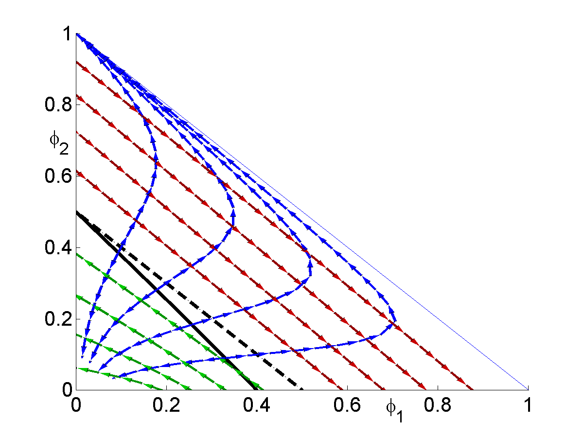
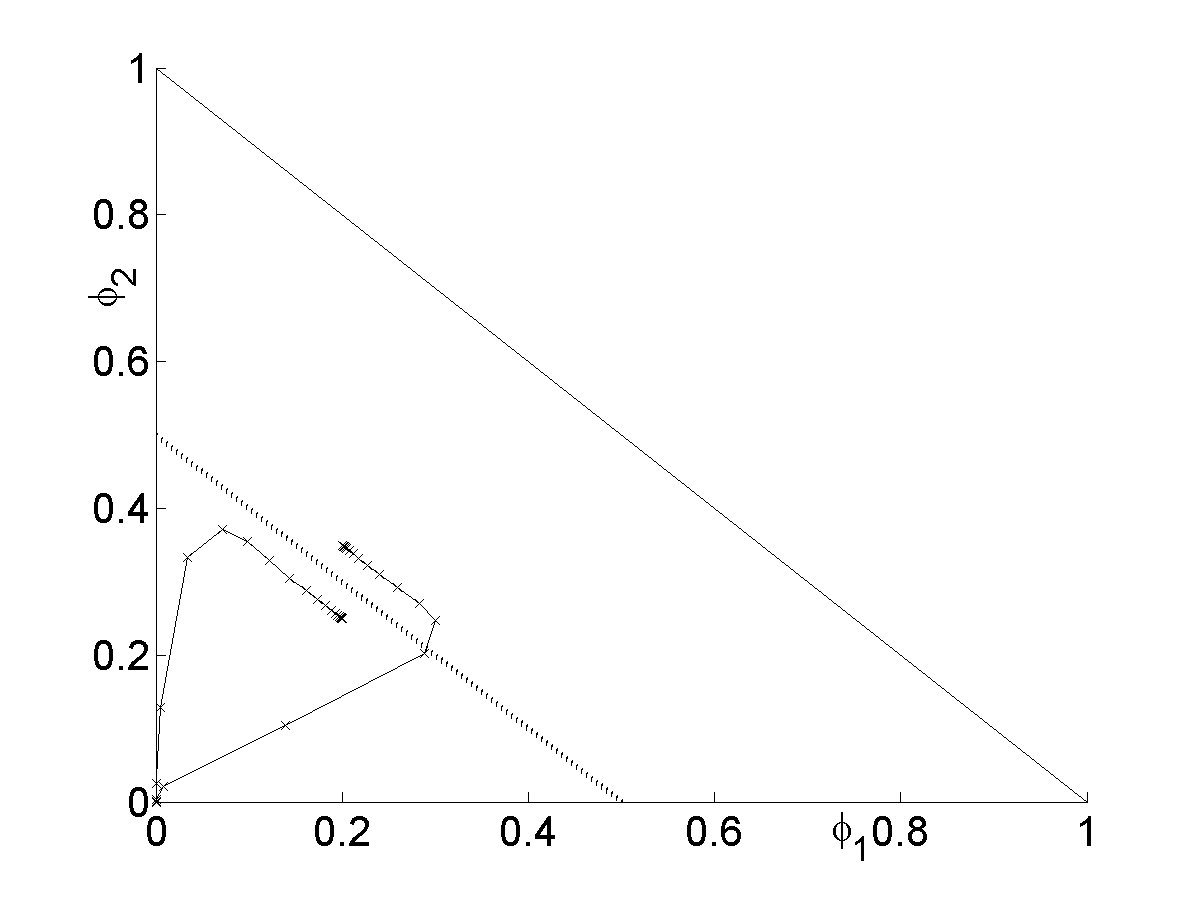
Figure 1: Phase space of Example 1 with parameters (45). Left: Integral curves in the $\phi_{1}\phi_{2}-$coordinate plane: First family (crossing all lines with constant $\phi$) and second family (connecting the axis). The integral curves point into the direction of increasing eigenvalues; contact manifold (dashed), inflection manifold of the first family (solid). Right: Solution of Riemann problems $RP(O,(0.2,0.25))$, $\mathrm{RP}(O,(0.2,0.35))$ by a finite difference method (low resolution).

5 Quasi-umbilic point

The best examined cases of the loss of hyperbolicity are related to an “umbilic point” [20, 25, 29], which is an isolated point where strict hyperbolicity fails. A description of new types of isolated points with loss of hyperbolicity is given in [27]. In particular, if there is a connected set of points with loss of hyperbolicity, then more refined characterizations are needed. For instance, a generalization of the umbilic point is the coincidence point.

Definition 6.

A point $\Phi$ is called a coincidence point of the PDE (1) with flux function $\boldsymbol{f}(\Phi)$ if the eigenvalues of the Jacobian matrix $\boldsymbol{J}(\Phi)$ of the flux function coincide at this point. We say that a coincidence point $\Phi^{*}$ is an umbilic point if it satisfies the following conditions:

(H1) The Jacobian matrix $\boldsymbol{J}(\Phi^{*})$ is diagonalizable.

(H2) There is a neighborhood $V$ of $\Phi^{\mathrm{\star}}$ such that $\boldsymbol{J}(\Phi)$ has distinct eigenvalues for all $\Phi\in V\backslash\{\Phi^{*}\}$.

Typically, we would expect that umbilic points are isolated coincidence points. However, the previous definition of an umbilic point may fail in either of the two conditions. Following [26], we classify an isolated coincidence point where condition (H1) fails as a quasi-umbilic point. It seems that the classification of quasi-umbilic points appears at the first time in [26], in [27] a detailed description is given.

Lemma 9.

There is a unique coincidence point on $\Phi\in\partial^{1}$. Upon the choice of parameters there may exist up to two coincidence points on $\Phi\in\partial^{2}$.

Proof.

By definition, a state $\Phi$ is a coincidence point if and only if $\lambda_{a}(\Phi)=\lambda_{b}(\Phi)$ holds. Namely, from the eigenvalue expression (36), one has a coincident point on axis $\Phi\in\partial^{1}$ if there exists some $\phi_{1}\in[0,\,1]$ such that $(1-n_{1}\phi_{1})u_{1}(\Phi)=u_{2}(\Phi)$ holds. Therefore, we must look for such a value $\phi_{1}$ which is a zero root of $R_{1}(\phi)-v_{\infty 2}/v_{\infty 1}=0$, where

$$R_{1}(\phi):=(1-n_{1}\phi)(1-\phi)^{n_{1}-n_{2}}.$$

Notice that by (S1) and (S2) the ratio $v_{\infty 2}/v_{\infty 1}$ is smaller than one and that the power $n_{1}-n_{2}$ is positive. Since $R_{1}(0)=1$, $R_{1}(1/n_{1})=0$ and $R_{1}^{\prime}(\phi)=-n_{1}(1-\phi)^{n_{1}-n_{2}}-(n_{1}-n_{2})(1-n_{1}\phi)(1-\phi)^{n_{1}-n_{2}-1}$ is negative for all $\phi\in[0,\,1/n_{1}]$, we conclude that $R_{1}(\phi)=v_{\infty 2}/v_{\infty 1}$ occurs at a single point, say $\phi^{u}$, which is the unique zero root of $R_{1}(\phi)-v_{\infty 2}/v_{\infty 1}=0$. Let us denote such a state as $Q_{1}:=(\phi^{u},\,0)^{T}$.

Similarly, for the axis $\Phi\in\partial^{2}$, from the eigenvalue expression (36), we look for a value $\phi_{2}\in[0,\,1]$ (while $\phi_{1}=0$) which is a zero root of $R_{2}(\phi)-v_{\infty 1}/v_{\infty 2}=0$, where

$$R_{2}(\phi):=(1-n_{2}\phi)(1-\phi)^{n_{2}-n_{1}},\qquad\phi\neq 1.$$

Notice that $R_{2}(0)=1$ and $R_{2}(1/n_{2})=0$ hold, and since $n_{1}>n_{2}>1$, in the limit $\lim_{\phi\rightarrow 1-}R_{2}(\phi)=-\infty$ holds. Moreover, $R_{2}(\phi)$ is positive for $\phi\in[0,\,1/n_{2})$ and negative for $\phi\in(1/n_{2},\,1)$. As the ratio $v_{\infty 1}/v_{\infty 2}$ is larger than one, there is no coincidence point if $R_{2}(\phi)$ is always smaller than such a ratio. For $\phi\in[0,\,1)$ we have

$$R_{2}^{\prime}(\phi) = -n_{2}(1-\phi)^{n_{2}-n_{1}}-(n_{1}-n_{2})(1-n_{2}\phi)(1-\phi)^{n_{2}-n_{1}-1}$$

$$= [-n_{2}(1-\phi)+(n_{2}-n_{1})(1-n_{2}\phi)](1-\phi)^{n_{2}-n_{1}-1}.$$

Thus, a single extremum of $R(\phi)$ occurs at

$$\phi^{m}:=\displaystyle{\frac{{\displaystyle{n_{1}-2n_{2}}}}{{\displaystyle{(n_{1}-n_{2}-1)n_{2}}}}}$$ (46)

There is one single coincidence point on the axis if $R_{2}(\phi^{m})=v_{\infty 1}/v_{\infty 2}$. The existence of two coincidence points occurs if $R_{2}(\phi^{m})$ is larger than $v_{\infty 1}/v_{\infty 2}$; say $Q_{2}:=(0,\,\phi^{u}_{2})^{\mathrm{T}}$, $Q_{3}:=(0,\,\phi^{u}_{3})^{\mathrm{T}}$ where $R_{2}(\phi^{u}_{2})=R_{2}(\phi^{u}_{3})=v_{\infty 1}/v_{\infty 2}$. ∎

The necessary and sufficient conditions for coincidence points on $\partial^{2}$ are difficult to evaluate. Let us define the ratio $W:=v_{\infty 1}/v_{\infty 2}$. On the one hand we know that $V$ exceeds one due to condition (S1). On the other hand the powers $n_{1}$, $n_{2}$ are also free parameters. Some calculations are possible if the difference between $n_{1}$ and $n_{2}$ is a natural number. For example, for $n_{1}-n_{2}=1$, there are two coincidence points if $n_{2}>W$; for $n_{1}-n_{2}=2$, there are two coincidence points if $n_{2}>2(W+\sqrt{W^{2}-W})$; for $n_{1}-n_{2}=3$, there are two coincidence points if $4n_{2}^{3}-27W(n_{2}-1)^{2}>0$. The inequality $R_{2}(\phi_{m})<1$ holds for powers satisfying $n_{2}+1<n_{1}<2n_{2}$, and for $\phi_{m}$ definied in (46). In this case there are not coincidences on the axis $\partial^{2}$.

For $\Phi=(\phi,0)^{\mathrm{T}}$ the Jacobian matrix is an upper triangular matrix and for $\Phi=(0,\phi)^{\mathrm{T}}$ a lower triangular matrix. In both cases the Jacobian matrix is diagonalizable. In view of Definition (6), condition (H2) is satisfied, but (H1) not necessarily. Given that the diagonalization is valid for all $\Phi\in\partial^{1}$, the coincidence point $Q_{1}=(\phi^{u},0)^{\mathrm{T}}$ is a quasi-umbilic point, where the Jacobian matrix has the form

$$\begin{pmatrix}c_{\sigma}&*\\ 0&c_{\sigma}\end{pmatrix}$$

is a Jordan block with $*\neq 0$ and therefore not diagonalizable. This means that (H1) is violated, but (H2) is satisfied. Therefore, from Lemma 9 we have the following result.

Corollary 1.

Any isolated coincidence point on the boundary turns out to be quasi-umbilic.

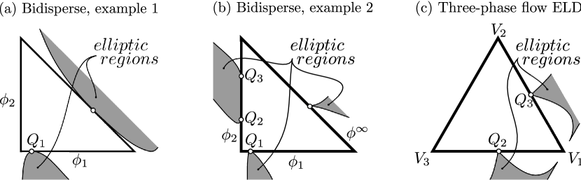
Figure 2: Extended domains. Concentration and saturation triangles are marked by a bold solid line, shaded regions contain states with complex eigenvalues of the flux Jacobian. In (a) the Example 1 reveals two quasi-umbilic points at the boundary of elliptic regions; the point $Q_{1}$ was detected by our analysis. In (b) the Example 2 shows the three quasi-umbilic points detected by the previous analysis, another one appears at the boundary of the elliptic regions. The plot in (c) represents the ELD where the two quasi-umbilic points also belong to the boundary of elliptic regions.

For illustration of the behavior of the coincidence points the flux functions (6) are continuously extended beyond the phase space by considering relative velocities (10) without the cut-off (9). The visualization in Fig. 2 shows that the identified quasi-umbilic point happens to belong to an elliptic/hyperbolic boundary; thus, it is clear that $\lambda_{1}(Q_{1})=\lambda_{2}(Q_{1})$ holds. Such a concept is introduced in [26], and here, their flux functions are also extended by letting the dominated quadratic terms to act outside the physical domain. In this case the quasi-umbilic points also belong to an elliptic/hyperbolic boundary, see Fig. 2 (c).

For the bidisperse model with parameter specifications (S1)–(S3) two general examples are considered. Besides Example 1 with parameter setting (45), Example 2 has the parameters

$$v_{1\infty}=1,v_{2\infty}=1/2,\qquad n_{1}=4.6,n_{2}=1.5.$$ (47)

For the ELD model (Equal-Lighter-Density fluids) case in Rodríguez-Bermúdez and Marchesin (2013) the parameters are chosen as $\rho_{1}=2.0>1.0=\rho_{2}=\rho_{3}$.

6 Shock classification of Hugoniot locus of origin

In this Section the types of shocks which are connected to the origin are classified. The shock classification of Definition 2 distinguishes three different types of admissible shocks, namely 1-Lax, 2-Lax and overcompressive shocks. The locations of the shocks on the Hugoniot $\mathcal{H}(O)$ of the origin $O=(0,\,0)^{T}$ are identified in Lemma 4; it includes in particular two contact manifolds. The shock classification builds on the eigenvalue analysis of Section 4 by comparing the shock speed and the eigenvalues in each state on the Hugoniot locus.

A key feature for the determination of the shock type consists of the order switch of the relative velocities at the threshold concentration $\phi^{\mathrm{x}}$,

$$\begin{cases}u_{1}(\Phi)>u_{2}(\Phi)\quad\text{for}\quad\phi\in[0,\phi^{\mathrm{x}}),\\ u_{1}(\Phi)=u_{2}(\Phi)\quad\text{for}\quad\phi\in\{\phi^{\mathrm{x}},\phi^{\infty}\},\\ u_{1}(\Phi)<u_{2}(\Phi)\quad\text{for}\quad\phi\in(\phi^{\mathrm{x}},\phi^{\infty}),\end{cases}$$ (48)

which is a direct consequence of the definition of the relative velocity (8), (9), together with the specifications (S1) and (S2).

A visual guide for the shock classification of shocks between the origin and states on the edges $\partial^{1}$ and $\partial^{2}$ is given by Fig. 3, where the shock speeds are compared to the characteristic speeds. The shock classification is essentially obtained by speed comparisons. In the following Theorem, the shock characterization is established for general parameter choices.

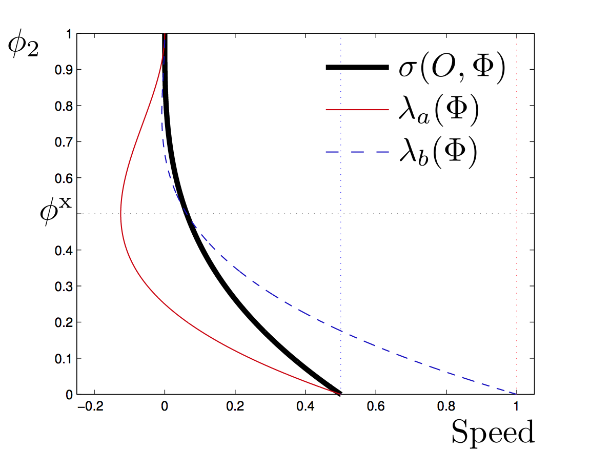
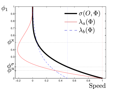
(a)	(b)

Figure 3: Eigenvalues and shock speeds of shocks from the origin to (a) the states $\Phi=(0,\,\phi)\in\partial^{2},\,\phi\in[0,\,1]$, (b) the states $\Phi=(\phi,\,0)\in\partial^{1},\,\phi\in[0,\,1]$. Bold solid curves represent the shock speed $\sigma(O,\,\Phi)$. The eigenvalues (characteristic speeds) given in (36) are represented as light solid curves for $\lambda_{a}(\Phi)$ and dashed curves for $\lambda_{b}(\Phi)$. The dotted horizontal lines represent heights corresponding to $\phi^{\mathrm{x}}$, $\phi^{\sigma}$, and $\phi^{u}$, ordered from top to bottom.

Theorem 2.

The Riemann problem

$$\mathrm{RP}(O,\Phi),\;\Phi\in\mathcal{H}(O)=\partial^{1}\cup\partial^{2}\cup\mathcal{C}(\Phi^{\mathrm{x}})\cup\mathcal{C}(\Phi^{\infty})$$

connecting the origin to a state of its Hugoniot locus is solved by a single shock of speed $\sigma=\sigma(O,\Phi)$, which can be classified as follows according to Definition 2.

Classification for $\Phi=(\phi_{1},0)^{\mathrm{T}}\in\partial^{1}$:

$$\begin{array}[]{rcl}\mbox{2-Lax: }&\lambda_{1,\,2}(\Phi)\,\leq\,\sigma\,<\,\lambda_{2}(O)\,\mbox{ and }\,\lambda_{1}(O)\,<\,\sigma&\,\mbox{ for }\,\phi_{1}\in(0,\,\phi^{\sigma}),\\ &\lambda_{1,\,2}(\Phi)\,\leq\,\sigma\,<\,\lambda_{2}(O)\,\mbox{ and }\,\lambda_{1}(O)\,=\,\sigma&\,\mbox{ for }\,\phi_{1}=\phi^{\sigma}.\\ \mbox{OC: }&\lambda_{1,\,2}(\Phi)\,<\,\sigma\,<\,\lambda_{1,\,2}(O)&\,\mbox{ for }\,\phi_{1}\in(\phi^{\sigma},\,\phi^{\mathrm{x}}).\\ \mbox{1-Lax: }&\lambda_{1}(\Phi)\,<\,\sigma\,<\,\lambda_{1,\,2}(O)\,\mbox{ and }\,\sigma\,=\,\lambda_{2}(\Phi)&\,\mbox{ for }\,\phi_{1}\in\{\phi^{\mathrm{x}},\phi^{\infty}\},\\ &\lambda_{1}(\Phi)\,<\,\sigma\,<\,\lambda_{1,\,2}(O)\,\mbox{ and }\,\sigma\,<\,\lambda_{2}(\Phi)&\,\mbox{ for }\,\phi_{1}\in(\phi^{\mathrm{x}},\,\phi^{\infty}).\\ \end{array}$$ (49)

The threshold value $\phi^{\sigma}$ is given as

$$\phi^{\sigma}=1-\,\,^{n_{1}}\!\!\!\!\sqrt{v_{\infty 2}/v_{\infty 1}}.$$ (50)

Classification for $\Phi=(0,\phi_{2})^{\mathrm{T}}\in\partial^{2}$:

$$\begin{array}[]{rcl}\mbox{1-Lax: }&\lambda_{1}(\Phi)\,<\,\sigma\,<\,\lambda_{1,\,2}(O)\,\mbox{ and }\,\sigma\,<\,\lambda_{2}(\Phi)&\,\mbox{ for }\,\phi_{2}\in(0,\phi^{\mathrm{x}}),\\ &\lambda_{1}(\Phi)\,<\,\sigma\,<\,\lambda_{1,\,2}(O)\,\mbox{ and }\,\sigma\,=\,\lambda_{2}(\Phi)&\,\mbox{ for }\,\phi_{2}\in\{\phi^{\mathrm{x}},\phi^{\infty}\}.\\ \mbox{OC: }&\lambda_{1,\,2}(\Phi)\,<\,\sigma\,<\,\lambda_{1,\,2}(O)&\,\mbox{ for }\,\phi_{2}\in(\phi^{\mathrm{x}},\,\phi^{\infty}).\\ \end{array}$$ (51)

Classification for $\Phi\in\mathcal{C}(\Phi^{\mathrm{x}})$:

$$\begin{array}[]{rcl}\mbox{1-Lax: }&\lambda_{1}(\Phi)\,<\,\sigma\,<\,\lambda_{1,\,2}(O)\,\mbox{ and }\,\sigma\,=\,\lambda_{2}(\Phi).\end{array}$$ (52)

Classification for $\Phi\in\mathcal{C}(\Phi^{\infty})$:

$$\begin{array}[]{rcl}\mbox{1-Lax: }&\lambda_{1}(\Phi)\,=\,\sigma\,<\,\lambda_{1,\,2}(O)\,\mbox{ and }\,\sigma\,=\,\lambda_{2}(\Phi).\end{array}$$ (53)

Strict inequalities in the shock type classification (49)-(53) mean that the corresponding shocks are not characteristic shocks. For instance, for $\Phi\in\partial^{1}$ there are no 1-Lax shocks characteristic at the left datum $O$.

Proof.

The proof is done in two main steps:
    1.- The first step is to relate the characteristic speeds $\lambda_{1,2}(O)$ and $\lambda_{a,b}(\Phi)$ to the shock speed $\sigma(O,\Phi)$ in dependence of the position of $\Phi$.
    2.- The second step consists in determining which shock classification applies according to Definition 2.

Table 1 gives an overview on the speed magnitudes for right states on the axes $\partial^{1}$ and $\partial^{2}$.

		$<\sigma(O,\Phi)$		$>\sigma(O,\Phi)$
$\partial^{1}:$	$\phi<\phi^{\sigma}$	$\lambda_{a,b}(\Phi)$	$\lambda_{1}(O)$		$\lambda_{2}(O)$	2-Lax
	$\phi\in(\phi^{\sigma},\phi^{\mathrm{x}}$)	$\lambda_{a,b}(\Phi)$			$\lambda_{1,2}(O)$	OC
	$\phi>\phi^{\mathrm{x}}$	$\lambda_{a}(\Phi)$		$\lambda_{b}(\Phi)$	$\lambda_{1,2}(O)$	1-Lax
$\partial^{2}:$	$\phi<\phi^{\mathrm{x}}$	$\lambda_{a}(\Phi)$		$\lambda_{b}(\Phi)$	$\lambda_{1,2}(O)$	1-Lax
	$\phi>\phi^{\mathrm{x}}$	$\lambda_{a,b}(\Phi)$			$\lambda_{1,2}(O)$	OC

Table 1: Shock classification on Hugoniot locus of origin for states on the axes $\partial^{1}$ and $\partial^{2}$. First column: Location on the axis. Second column: Characteristic speeds less than $\sigma(O,\Phi)$. Third column: Characteristic speeds larger than $\sigma(O,\Phi)$. Forth column: Shock type.

$\lambda_{2}(O)$ compared to $\sigma(O,\,\Phi)$ on $\partial^{1}$ and $\partial^{2}$

On the axes $\Phi\in\partial^{i}\backslash O$ the shock speed is limited as

$$\sigma(O,\Phi)=v_{i}(\Phi)<v_{\infty i}=\begin{cases}v_{\infty 1}=\lambda_{2}(O),&\quad\text{if}\quad i=1,\\ v_{\infty 2}=\lambda_{1}(O)<\lambda_{2}(O),&\quad\text{if}\quad i=2,\end{cases}$$ (54)

since the shock speed

$$\sigma(O,\,\Phi)=v_{i}(\Phi)=(1-\phi_{i})u_{i}(\Phi)=v_{\infty i}(1-\phi_{i})^{n_{i}},\quad i=1,\,2,$$

is monotonically decreasing on both axes $\partial^{1}$ and $\partial^{2}$. (Note that (54) excludes 2-Lax shocks on edge $\partial^{2}$.)

$\lambda_{a}(\Phi)$ compared to $\sigma(O,\,\Phi)$ on $\partial^{1}$ and $\partial^{2}$

The eigenvalue $\lambda_{a}(\Phi)$ as specified in (36) leads to common properties for both axes. For all points $\Phi\in\partial^{i}\backslash O,\;i\in\{1,2\}$, along the axes one has

$$\begin{split}\lambda_{a}(\Phi)&=[1-(1+n_{i})\phi_{i}]u_{i}(\Phi)\\ &<(1-\phi_{i})u_{i}(\Phi)=v_{i}(\Phi)=\sigma(O,\Phi),\quad i=1,2,\end{split}$$ (55)

due to properties that apply on the axes, namely, the speed convertibility (31) and the shock speed (29).

$\lambda_{b}(\Phi)$ compared to $\sigma(O,\,\Phi)$ on $\partial^{1}$ and $\partial^{2}$

The composition of the eigenvalue $\lambda_{b}(\Phi)$ depends on the inequality (48) between the relative velocities $u_{1}(\Phi)$ and $u_{2}(\Phi)$, and induces quite different behaviors on the edges. On the axis $\partial^{1}$ the eigenvalue $\lambda_{b}(\Phi)$ behaves as

$$\begin{cases}\lambda_{b}(\Phi)<\sigma(O,\,\Phi)\quad\text{for}\quad\phi_{1}\in(0,\,\phi^{\mathrm{x}}),\\ \lambda_{b}(\Phi)=\sigma(O,\,\Phi)\quad\text{for}\quad\phi_{1}\in\{\phi^{\mathrm{x}},\phi^{\infty}\},\\ \lambda_{b}(\Phi)>\sigma(O,\,\Phi)\quad\text{for}\quad\phi_{1}\in(\phi^{\mathrm{x}},\,\phi^{\infty}),\end{cases}$$ (56)

because on $\partial^{1}$, the inequalities (48) between $u_{1}(\Phi)$ and $u_{2}(\Phi)$ implies that for the interval $\phi_{1}\in[0,\,\phi^{\mathrm{x}})$ the eigenvalue (36) satisfies

$$\lambda_{b}(\Phi)=u_{2}(\Phi)-\phi_{1}u_{1}(\Phi)<(1-\phi_{1})u_{1}(\Phi)=\sigma(O,\,\Phi),$$

and for the other interval, where $\phi_{1}\in(\phi^{\mathrm{x}},\,\phi^{\infty}]$, the inequality sign switches.

On the axis $\partial^{2}$ one has

$$\begin{cases}\lambda_{b}(\Phi)>\sigma(O,\Phi)\quad\text{for}\quad\phi_{2}\in[0,\phi^{\mathrm{x}}),\\ \lambda_{b}(\Phi)=\sigma(O,\Phi)\quad\text{for}\quad\phi_{2}\in\{\phi^{\mathrm{x}},\phi^{\infty}\},\\ \lambda_{b}(\Phi)<\sigma(O,\Phi)\quad\text{for}\quad\phi_{2}\in(\phi^{\mathrm{x}},\phi^{\infty}),\end{cases}$$ (57)

since, from the inequalities (48) for $\phi_{2}\in[0,\phi^{\mathrm{x}})$, one obtains

$$\lambda_{b}(\Phi)=u_{1}(\Phi)-\phi_{2}u_{2}(\Phi)>(1-\phi_{2})u_{2}(\Phi)=\sigma(O,\,\Phi)$$

and for $\phi\in(\phi^{\mathrm{x}},\phi^{\infty}]$ the inequality sign switches.

On the edge $\partial^{2}$ the value of $\lambda_{b}(\Phi)$ determines whether the shock is 1-Lax or over-compressive. The shock type is decided by the relative magnitudes of $u_{1}(\Phi)$ contra $u_{2}(\Phi)$: The equality $u_{1}(\Phi)=u_{2}(\Phi)$ only holds for $\phi_{2}=\phi^{\mathrm{x}}$ (and $\phi_{2}=\phi^{\infty}$). On edge $\partial^{1}$ there is a coincidence of eigenvalues, see also Lemma 9.

$\lambda_{1}(O)$ compared to $\sigma(O,\,\Phi)$ on $\partial^{1}$ and $\partial^{2}$

Note that, along both axes $\sigma(O,\Phi)$ is a monotonically decreasing function with $\sigma(O,\Phi^{\infty})=0$. By (54) is assured that $\sigma(O,\Phi)<\lambda_{1}(O)$ holds for all states on the axis $\partial^{2}\backslash O$. However, this does not hold for all states on the axis $\partial^{1}\backslash O$.

Since $\lim_{\varepsilon\rightarrow 0}\sigma(O,(\varepsilon,0))=\lambda_{2}(O)>\lambda_{1}(O)>0$ on the axis $\partial^{1}$, there exists a state $\Phi^{\sigma}=(\phi^{\sigma},0)^{\mathrm{T}}$ such that $\sigma(O,\Phi^{\sigma})=\lambda_{1}(O)$. In this state $\Phi^{\sigma}$ the equality

$$\sigma(O,\Phi^{\sigma})=v_{1}(\Phi^{\sigma})=v_{\infty 1}(1-\phi_{\sigma})^{n_{1}}=v_{\infty 2}=\lambda_{1}(O)$$

holds, from which the characterization of $\phi^{\sigma}$ by (50) can be deduced. The shock speed $\sigma(O,\Phi)$ relates to $\lambda_{1}(O)$ in dependence of $\phi^{\sigma}$ as

$$\begin{cases}\sigma(O,\,\Phi)>\lambda_{1}(O)\quad\text{for}\quad\phi_{1}\in[0,\,\phi^{\sigma}),\\ \sigma(O,\,\Phi)=\lambda_{1}(O)\quad\text{for}\quad\phi_{1}=\phi^{\sigma},\\ \sigma(O,\,\Phi)<\lambda_{1}(O)\quad\text{for}\quad\phi_{1}\in(\phi^{\sigma},\,\phi^{\infty}].\end{cases}$$ (58)

Together with the previously established (54), (55) and (56) the discrimination (58) implies that, on the axis $\partial^{1}$, for $\phi<\Phi^{\sigma}$ there is a 2-Lax shock, whereas for $\Phi^{\sigma}<\phi<\phi^{\mathrm{x}}$ the shock is over-compressive.

By (55), (56), for $\phi\in(\phi^{\mathrm{x}},\phi^{\infty})$, on axis $\partial^{1}$ there is a clear separation between the shock speeds:

$$\lambda_{1}(\Phi)=\lambda_{a}(\Phi)<\sigma(O,\Phi)<\lambda_{b}(\Phi)=\lambda_{2}(\Phi).$$ (59)

This separation allows an association of the eigenvalues according to (37). The same way, by (55), (57) for $\phi\in(0,\phi^{\mathrm{x}})$ on $\partial^{2}$ there is a clear separation between the shock speeds (59) that establishes the eigenvalues order (37). For $\phi\in(\phi^{\mathrm{x}},\phi^{\infty})$ there is no clear eigenvalue separation, which however does not affect the fact that the shock is over-compressive.

Now we are able to conclude the shock classification on the axes: Putting the inequalities (54), (55), (57) together gives the shock classification (51) for right states on the axis $\partial^{2}$. Putting the inequalities (54), (55), (56), (58) together gives the shock classification (49) for right states on the axis $\partial^{1}$.

Contact manifold $\mathcal{C}(\Phi^{\mathrm{x}})$

The shock classification for states on the contact manifold $\Phi\in\mathcal{C}(\Phi^{\mathrm{x}})$ assures that all states are connected to the origin by a 1-Lax shock: Since the functions $v_{1}(\Phi)$ and $v_{2}(\Phi)$ take their maximum in the origin $O$ and the origin is not part of the contact manifold, one has the strict inequality

$$\sigma(O,\Phi)=v_{1}(\Phi^{\mathrm{x}})<v_{\infty 1}=\lambda_{1}(O)<v_{\infty 2}=\lambda_{2}(O).$$ (60)

By the eigenvalue characterization (35) for states on $\mathcal{C}(\Phi^{\mathrm{x}})$, and noting that $\Delta_{\Phi}>0$ for all $\Phi\in\mathcal{C}(\Phi^{\mathrm{x}})$, one gets

$$\lambda_{1}(\Phi)<\sigma(O,\Phi)=v_{1}(\Phi)=\lambda_{2}(\Phi)$$ (61)

for all $\Phi\in\mathcal{C}(\Phi^{\mathrm{x}})$. The properties (60) and (61) are summarized in the shock classification (52).

Contact manifold $\partial^{\infty}=\mathcal{C}(\Phi^{\infty})$

For states on the maximum packing manifold $\Phi\in\partial^{\infty}$ one has vanishing eigenvalues,

$$0=\lambda_{1}(\Phi)=\lambda_{2}(\Phi)=\sigma(O,\Phi)<\lambda_{1}(O)<\lambda_{2}(O),$$

which leads to classification (53). ∎

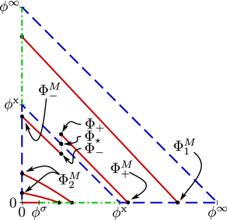
Figure 4: Different shock types for states connected to the origin. Continuous curves are 2-Lax shocks, dashed curves are 1-Lax shocks and dotted-dashed are over-compressive shocks. The Hugoniot locus of the origin comprises the three edges and the contact manifolds $\mathcal{C}(\Phi^{\mathrm{x}})$, $\mathcal{C}(\Phi^{\infty})$. Also some 2-Lax shock curves from arbitrarily chosen generic points $\Phi_{1}^{M}$, $\Phi_{2}^{M}$, $\Phi_{-}^{M}$ and $\Phi_{+}^{M}$ are indicated. Reference values on the horizontal axis $\partial^{1}$ are $\phi^{\sigma}$, $\phi^{\mathrm{x}}$ and $\phi^{\infty}$, on the vertical axis $\partial^{2}$ are $\phi^{\mathrm{x}}$ and $\phi^{\infty}$.

Figure 4 displays the different shock types for states connected with the origin, as elaborated in Theorem 2. The 1-Lax states of $\mathcal{H}(O)$ are shown as dashed lines.

States on the contact manifold $\mathcal{C}(\Phi^{\mathrm{x}})$ satisfy the 1-Lax conditions being characteristic in the second family at the right state. In the same manner, the states on the maximum packing $\mathcal{C}(\Phi^{\infty})=\partial^{\infty}$ satisfy to be 1-Lax shocks which are characteristic at the right state with respect to both families. On the edge $\partial^{2}$, at $\Phi^{\mathrm{x}}=(0,\,\phi^{\mathrm{x}})^{\mathrm{T}}$ and $\Phi^{\infty}=(0,\,\phi^{\infty})^{\mathrm{T}}$ the shocks are 1-Lax and characteristic at the right states, say $\sigma(O,\,\Phi^{\mathrm{x}})=\lambda_{2}(\Phi^{\mathrm{x}})$ and $\sigma(O,\,\Phi^{\infty})=\lambda_{2}(\Phi^{\infty})$. On the edge $\partial^{1}$, at $\Phi^{\mathrm{x}}=(\phi^{\mathrm{x}},\,0)^{\mathrm{T}}$, $\Phi^{\sigma}=(\phi^{\sigma},\,0)^{\mathrm{T}}$ and $\Phi^{\infty}=(\phi^{\infty},\,0)^{\mathrm{T}}$ the shocks are 2-Lax, over-compressive and 1-Lax, respectively, being characteristic at left or right states, say $\sigma(O,\,\Phi^{\mathrm{x}})=\lambda_{1}(O)$, $\sigma(O,\,\Phi^{\sigma})=\lambda_{2}(\Phi^{\sigma})$ and $\sigma(O,\,\Phi^{\infty})=\lambda_{2}(\Phi^{\infty})$. Several states located in Fig. 3 (b) have characteristic shocks: If $\Phi\in\mathcal{C}(\Phi^{\mathrm{x}})$ then the shock is right characteristic for the second family, if $\phi=\phi^{\infty}$ then it is characteristic for both families, and if $\Phi=(0,\,\phi^{\sigma})^{\mathrm{T}}$ then the shock is 2-Lax but left characteristic in the first family.

7 Riemann problems

In this Section, we construct the solution of the Riemann problems $\mathrm{RP}(O,\,\Phi)$ and $\mathrm{RP}(\Phi,\,\Phi^{\infty})$, where $O=(0,\,0)^{\mathrm{T}}$, $\Phi^{\infty}\in\partial^{\infty}$, and $\Phi\in\mathcal{D}_{\Phi^{\infty}}$ is a generic right or left state in the phase space. These Riemann problems are derived from the standard initial condition (16).

7.1 The Riemann problem $\mathrm{RP}(O,\,\Phi)$

The behavior of solutions to the Riemann problem $\mathrm{RP}(O,\Phi)$ depends on the position of $\Phi$ in the interior of $\mathcal{D}_{\Phi^{\infty}}$ with respect to the contact manifold $\mathcal{C}(\Phi^{\mathrm{x}})$, which splits the domain into two regions:

$$\mathcal{D}_{\mathrm{x}}^{-} := \{\Phi\in\mathcal{D}_{\Phi^{\infty}}\,:\,\phi<\phi^{\mathrm{x}}\},$$

$$\mathcal{D}_{\mathrm{x}}^{+} := \{\Phi\in\mathcal{D}_{\Phi^{\infty}}\,:\,\phi>\phi^{\mathrm{x}}\},$$

where $\mathcal{C}(\Phi^{\mathrm{x}})=\mathrm{cl}\bigl{(}\mathcal{D}_{\mathrm{x}}^{-}\bigr{)}\cap\mathrm{cl}\bigl{(}\mathcal{D}_{\mathrm{x}}^{+}\bigr{)}$ marks the intersection of the closures of those two regions. The main difference between both domains is the opposite direction of the characteristic speeds on the integral curves. In $\mathcal{D}_{\mathrm{x}}^{-}$ the second eigenvalue increases from the edge $\partial^{1}$ to the edge $\partial^{2}$, and, reversely, in $\mathcal{D}_{\mathrm{x}}^{+}$ the second eigenvalue increases from the edge $\partial^{2}$ to the edge $\partial^{1}$. See the orientation of the second rarefactions in Fig. 1, where the arrows point into the directions of increasing eigenvalues.

A Riemann solution from $O$ to any state $\Phi$ in $\mathcal{D}_{\Phi^{\infty}}$ generally consists of a 1-Lax shock followed by a 2-Lax shock. For $\Phi$ belonging to $\mathcal{D}_{\mathrm{x}}^{-}$ the middle state that intersects the 1-wave with the 2-wave is denoted by $\Phi_{-}^{M}$, and for $\Phi$ belonging to $\mathcal{D}_{\mathrm{x}}^{+}$ the middle state is denoted by $\Phi_{+}^{M}$. In both cases the middle state $\Phi^{M}$ belongs to the 1-Lax locus of the origin $O$. Since both waves are shocks any middle state $\Phi_{+}^{M}$ or $\Phi_{-}^{M}$ is located at $\mathcal{H}(\Phi)\cup\mathcal{H}(O)$. It turns out that $\Phi_{+}^{M}$ belongs to the edge $\partial^{1}$ and $\Phi_{-}^{M}$ belongs to the edge $\partial^{2}$.

For a right state $\Phi\in\mathcal{D}_{\mathrm{x}}^{-}$ the solution of $RP(O,\,\Phi)$ comprises the 1-Lax shock from $O$ to a state $\Phi^{M}=(0,\,\phi^{M})^{T}$ such that $\phi^{M}\in(0,\,\phi^{\mathrm{x}})$ and the 2-Lax shock from $\Phi^{M}$ to $\Phi$. Similarly, for a right state $\Phi\in\mathcal{D}_{\mathrm{x}}^{+}$ the solution of $RP(O,\,\Phi)$ comprises the 1-Lax shock from $O$ to a state $\Phi^{M}=(\phi^{M},\,0)^{T}$ such that $\phi^{M}\in(\phi^{\mathrm{x}},\,\phi^{\infty})$ and the 2-Lax shock from $\Phi^{M}$ to $\Phi$. Such cases are depicted in Fig. 4; the former as $\Phi_{-}\in\mathcal{D}_{\mathrm{x}}^{-}$ and the latter as $\Phi_{+}\in\mathcal{D}_{\mathrm{x}}^{+}$.

The solution of the Riemann problem $RP(O,\,\Phi)$ with $\Phi$ on the Hugoniot locus of $O$ comprises a single shock from $O$ to $\Phi$ with a classification that depends on the position of $\Phi$ and is elaborated in Theorem 2:

1. For $\Phi=(\phi,\,0)^{\mathrm{T}}$ with $\phi\in(\phi^{\sigma},\,\phi^{\mathrm{x}})$ the shock is over-compressive,

2. For $\Phi=(0,\,\phi)^{\mathrm{T}}$ with $\phi\in(\phi^{\mathrm{x}},\,\phi^{\infty})$ the shock is over-compressive,

3. For $\Phi=(\phi,\,0)^{\mathrm{T}}$ with $\phi\in(0,\,\phi^{\sigma})$ the shock is 2-Lax,

4. For any other $\Phi$ in $\mathcal{H}(O)$ the shock is 1-Lax.

For a state $\Phi\in\mathcal{C}(\Phi^{\mathrm{x}})$, the solution of the Riemann problem $RP(O,\,\Phi)$ consists of a single 1-Lax shock from $O$ to $\Phi$. The two consecutive shocks from $O$ to $(0,\,\phi^{\mathrm{x}})^{T}$ and from $(0,\,\phi^{\mathrm{x}})^{\mathrm{T}}$ to $\Phi$ have both the same speed $v_{1}(\phi^{\mathrm{x}})=v_{2}(\phi^{\mathrm{x}})$, which in turn is the same speed of the direct shock from $O$ to $\Phi$. Since all these shocks have the same speed, the middle state $(0,\,\phi^{\mathrm{x}})^{\mathrm{T}}$ is “invisible” in the solution profile in the physical space; this is because of Lemma 1. Therefore, the solution structure for $\Phi\in\mathcal{D}_{\Phi^{\infty}}$ is represented as

$$O\xrightarrow{\mathrm{1-Lax}}\Phi^{M}\xrightarrow{\mathrm{2-Lax}}\Phi.$$

For $\Phi\in\mathcal{C}(\Phi^{\mathrm{x}})$ the middle state $\Phi^{M}$ may assume any other state on the same contact manifold and even collapse with $\Phi$.

Please refer to Fig. 4 and notice that as any $\Phi_{-}\in\mathcal{D}_{\mathrm{x}}^{-}$ tends to a $\Phi\in\mathcal{C}(\Phi^{\mathrm{x}})$ the middle state $\Phi_{-}^{M}$ tends to $(0,\,\phi^{\mathrm{x}})^{T}$. Similarly, as $\Phi_{+}\in\mathcal{D}_{\mathrm{x}}^{+}$ tends to a $\Phi\in\mathcal{C}(\Phi^{\mathrm{x}})$, the state $\Phi_{+}^{M}$ tends to $(\phi^{\mathrm{x}},\,0)^{\mathrm{T}}$. Thus, we notice a continuous dependence of solutions to the Riemann problem $RP(O,\,\Phi)$ on the right datum.

7.2 The Riemann problem $RP(\Phi,\,\Phi^{\infty})$

In this Section, the dependence of the solution structure on the exponents $n_{1}$ and $n_{2}$ is illustrated by two examples, Example 1 and Example 2 with the corresponding parameter setting (45) and (47), respectively. In the Example 1, the solution consists of a simple 1-wave comprising a shock followed by a rarefaction or a single rarefaction. The solution structure of Example 2 depends on the existence of one or two detached inflection curves for the first characteristic family. As $\mathcal{C}(\Phi^{\infty})$ is a contact manifold, the goal is to consider a generic state $\Phi\in\mathcal{D}_{\Phi^{\infty}}$ from which waves reaching any state in $\Phi^{\infty}\in\partial^{\infty}$ are constructed.

Construction for Example 1. The construction for Example 1 can be orientated by the integral curves and the inflection manifold in Figure 1. In Figure 1 (a) the inflection manifold $\mathcal{I}_{1}$ of the first family is shown as a solid curve, which is almost a straight line, connecting the states $\Phi^{\diamond}_{1}=(0.4,\,0)^{\mathrm{T}}$ and $\Phi^{\diamond}_{2}=(0,\,0.5)^{\mathrm{T}}$, compare Lemma 7. Therefore, a wave curve starting at a state on the upper-right hand side of $\mathcal{I}_{1}$ follows a centered rarefaction of the first family until the maximum packing manifold $\partial^{\infty}$ is reached. The final rarefaction point is $(0,\,1)^{\mathrm{T}}$, unless the starting state is on the $\partial^{1}$ axis, in such a case, the final rarefaction point is $(1,\,0)^{\mathrm{T}}$.

The characteristic velocities near the contact manifold $\mathcal{C}(\Phi^{\infty})$ are close to zero, and the characteristic directions are close to $r_{2}=r_{1}=(1,\,-1)^{\mathrm{T}}$, see (44). If the left state $\Phi$ is on the lower-left side of the inflection $\mathcal{I}_{1}$ then the wave is obtained by a backward 1-wave construction. Namely, all shocks from a state $\Phi$ at the lower-left hand side of $\mathcal{I}_{1}$ are connected to a state $\Phi^{M}\in\mathcal{H}(\Phi)$ on the right of $\mathcal{I}_{1}$ satisfying $\sigma(\Phi,\,\Phi^{M})=\lambda_{1}(\Phi^{M})$. Therefore, the solution for such a state $\Phi$ comprises the 1-Lax shock from $\Phi$ to $\Phi^{M}$ which is characteristic at $\Phi^{M}$, and the rarefaction curve from $\Phi^{M}$ to $(0,\,1)^{\mathrm{T}}$, or $(1,\,0)^{\mathrm{T}}$ if $\Phi$ belongs to $\partial^{1}$.

Construction of Example 2. The construction of Example 2 is visualized in Figure 5. The integral curves of the first family change their growth direction at two detached parts of the inflection manifold $\mathcal{I}_{1}$, namely $\mathcal{T}$ and $\mathcal{B}$, see Figure 5 (a). This growth direction change is the key in the distinct structure of the solution of $RP(\Phi,\,\Phi^{\infty})$ solutions in both Examples.

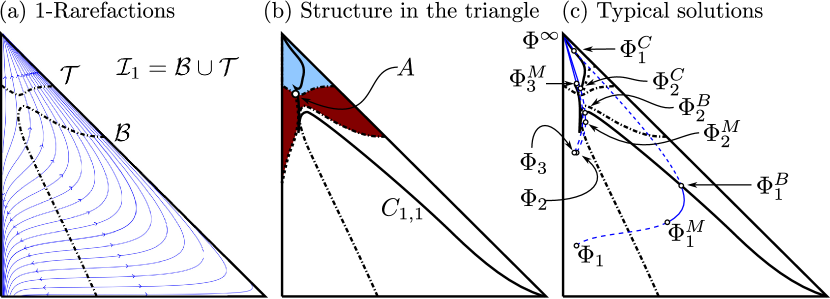
Figure 5: Curves of Example 2. In (a) the first family rarefaction curves are plotted as continuous curves, the arrows point into the direction of increasing eigenvalues. The dash-dotted curves are the inflection manifold $\mathcal{I}_{1}$ splitted into the two branches $\mathcal{T}$ and $\mathcal{B}$. In (b) the solid curve $C_{1,1}$ is the double-contact of the first family (notice the two components, one in the light region and one another in the white region); $A$ is the state where a limit shock curve from $\mathcal{T}$ does not cross $\mathcal{B}$. In the presentation of the wave curve solutions in (c) the continuous curves correspond to rarefaction fans and the dashed curves correspond to shock waves.

In Fig. 5 (b) the light and dark shaded regions represent right states $\Phi$ for which the solutions are similar to that of Example 1:

1. When the states belong to the upper corner above $\mathcal{T}$ inside the light shaded region, then the wave curve comprises a single 1-rarefaction connecting the state $\Phi$ moving along increasing eigenvalues $\lambda_{1}$ towards $\Phi^{\infty}=(1,\,0)^{\mathrm{T}}$;

2. For a left state $\Phi$ in the dark shaded region, a characteristic 1-Lax shock to a middle state in the light shaded region crosses $\mathcal{T}$, from this middle state a first family rarefaction follows to the maximum package concentration.

The construction of $RP(\Phi,\,\Phi^{\infty})$ solutions for $\Phi$ in the white region of Figure 5 (b) is outlined in the sequel. There are three cases of right characteristic 1-Lax shocks that connect a state $\Phi$ to a state $\Phi^{M}\in\mathcal{H}(\Phi)$ such that $\sigma(\Phi,\,\Phi^{M})=\lambda_{1}(\Phi^{M})$ :

(1) The shock curve crosses once $\mathcal{B}$;

(2) The shock curve crosses once $\mathcal{T}$;

(3) The shock curve crosses twice $\mathcal{B}$ and once $\mathcal{T}$.

In Figure 5 (c) the left states of the cases (1) are represented by $\Phi_{1}$ and $\Phi_{2}$, the case (2) is represented by point 2 above and, case (3) is represented by $\Phi_{3}$. The wave curves starting from $\Phi_{1}$, $\Phi_{2}$ and $\Phi_{3}$ have the following structure:

$$\Phi_{1}\xrightarrow{\mathrm{1-Lax}}\big{|}\Phi_{1}^{M}\xrightarrow{\mathrm{1-rar}}\Phi_{1}^{B}\big{|}\xrightarrow{\mathrm{1-Lax}}\big{|}\Phi_{1}^{C}\xrightarrow{\mathrm{1-rar}}\Phi^{\infty},$$ (62)

$$\Phi_{2}\xrightarrow{\mathrm{1-Lax}}\big{|}\Phi_{2}^{M}\xrightarrow{\mathrm{1-rar}}\Phi_{2}^{B}\big{|}\xrightarrow{\mathrm{1-Lax}}\big{|}\Phi_{2}^{C}\xrightarrow{\mathrm{1-rar}}\Phi^{\infty},$$ (63)

$$\Phi_{3}\xrightarrow{\mathrm{1-Lax}}\big{|}\Phi_{3}^{M}\xrightarrow{\mathrm{1-rar}}\Phi^{\infty},$$ (64)

where the symbol $\big{|}$ indicates where a shock is characteristic. For case (3) the construction of the shock curves proceeds as before, namely a 1-Lax shock followed by a 1-rarefaction connecting a middle state $\Phi^{M}$ in the light shade region in Fig. 5 (b) with $\Phi^{\infty}$. For case (i), with $i=1$ or $2$, the characteristic shock $(\Phi_{i},\,\Phi_{i}^{M})$ precedes a 1-rarefaction from $\Phi_{i}^{M}$ towards $\mathcal{B}$ at a state $\Phi_{i}^{B}$ on $C_{1,1}$, from there another 1-Lax left and right characteristic shock connects to a state $\Phi_{i}^{C}$ on the other side of $C_{1,1}$. From $\Phi_{i}^{C}$ the wave curve is terminated by the 1-rarefaction to $\Phi^{\infty}$.

If the state $\Phi_{2}$ is approximated to a state $\Phi_{3}$ then a continuous change in the solution profile is observed such that the wave group (63) collapses to the wave group (64). Indeed, if $\Phi_{2}$ comes closer to $\Phi_{3}$, then $\Phi_{2}^{M}$ comes closer to $\Phi_{2}^{B}$ and $\Phi_{2}^{C}$ to $\Phi_{3}^{M}$ in such a way that the shock speeds $\sigma(\Phi_{2},\,\Phi_{2}^{M})$ and $\sigma(\Phi_{2}^{B},\,\Phi_{2}^{C})$ approximate $\sigma(\Phi_{3},\,\Phi_{3}^{M})$, until, in the limit, the 1-rarefaction wave from $\Phi_{2}^{M}$ to $\Phi_{2}^{B}$ disappears.

References

- [1] A. Azevedo, D. Marchesin, B. Plohr and K. Zumbrun (2002) “Capillary instability in models for three-phase flow”, Zeitschrift für Angewandte Mathematik und Physik (ZAMP) 53: 713–746.
- [2] A.V. Azevedo, A.J. de Souza, F. Furtado, D. Marchesin and B. Plohr (2010) “The solution by the wave curve method of three-phase flow in virgin reservoirs”, Transp. Porous Media 83: 99–125.
- [3] D.K. Basson, S. Berres and R. Bürger (2009) “On models of polydisperse sedimentation with particle-size-specific hindered-settling factors”, Appl. Math. Modelling 33: 1815–1835.
- [4] S. Benzoni-Gavage and R. M. Colombo (2003) “An n-populations model for traffic flow”, Eur. J. Appl. Math. 14: 587–612.
- [5] S. Berres and R. Bürger (2007) “On Riemann problems and front tracking for a model of sedimentation of polydisperse suspensions”, ZAMM 87: 665–691.
- [6] S. Berres and R. Bürger (2008) “On the settling of a bidisperse suspension with particles having different sizes and densities”, Acta Mecanica 201: 47–62.
- [7] S. Berres, R. Bürger, K.H. Karlsen and E.M. Tory (2003) “Strongly degenerate parabolic-hyperbolic systems modeling polydisperse sedimentation with compression”, SIAM J. Appl. Math. 64: 41–80.
- [8] S. Berres, R. Ruiz-Baier, H. Schwandt and Elmer Tory (2011) “An adaptive finite-volume method for a model of two-phase pedestrian flow”, Netw. Het. Media 6: 401–423.
- [9] S. Berres and T. Voitovich (2009) “On the spectrum of a rank two modification of a diagonal matrix for lin-earized fluxes modelling polydisperse sedimentation”. In Tadmor, Eitan (ed.) et al., Hyperbolic problems. Theory, numerics and applications. Contributed talks. Proceedings of Hyp2008. American Mathematical Society (AMS). Proceedings of Symposia in Applied Mathematics 67(2): 409–418.
- [10] P.M. Biesheuvel (2000) “Particle segregation during pressure filtration for cast formation”, Chem. Eng. Sci. 55: 2595–2606.
- [11] R. Bürger, R. Donat, P. Mulet and C.A. Vega (2010) “Hyperbolicity analysis of polydisperse sedimentation models via a secular equation for the flux Jacobian”, SIAM Journal of Applied Mathematics 70: 2186–2213.
- [12] R. Bürger, K.H. Karlsen, E.M. Tory and W.L. Wendland (2002) “Model equations and instability regions for the sedimentation of polydisperse suspensions of spheres”, ZAMM Z. Angew. Math. Mech. 82: 699–722.
- [13] P. Castañeda, F. Furtado and D. Marchesin (2014) “On singular points for convex permeability models”, Hyperbolic Problems: Theory, Numerics, Applications, Proc. of Hyp2012, eds. F. Ancona, A. Bressan, P. Marcati, and A. Marson, AIMS Series on Appl. Math. 8: 415–422.
- [14] P. Castañeda, E. Abreu, F. Furtado and D. Marchesin. “On a universal structure for immiscible three-phase flow in virgin reservoirs”. (Submitted.)
- [15] C.M. Dafermos (2000) “Hyperbolic Conservation Laws in Continuum Physics”, Springer Verlag, Berlin.
- [16] A. de Souza (1992) “Stability of singular fundamental solutions under perturbations for flow in porous media”, Mat. Aplic. Comp. 11: 73–115.
- [17] R. Donat and P. Mulet (2010) “A secular equation for the Jacobian matrix of certain multi-species kinematic flow models”, Numer. Methods Partial Differential Equations 26: 159–175.
- [18] F.J. Fayers (1989) “Extension of Stone’s method 1 and conditions for real characteristic three-phase flow”, SPE Reservoir Engineering, 437–445.
- [19] F. Furtado (1989) Structural Stability of Nonlinear Waves for Conservation Laws, PhD Thesis, NYU.
- [20] E. Isaacson, D. Marchesin, B. Plohr and B. Temple (1988) “The Riemann problem near a hyperbolic singularity: the classification of solutions of quadratic Riemann problems”, SIAM J. Appl. Math. 48: 1009–1032.
- [21] E. Isaacson, D. Marchesin, B. Plohr and B. Temple (1992) “Multiphase flow models with singular Riemann problems”, Mat. Apl. Comput. 11: 147–166.
- [22] P. Lax (1957) “Hyperbolic systems of conservation laws II”, Commun. Pure Appl. Math. 10: 537–566.
- [23] A. Majda and R.L. Pego (1985) “Stable viscosity matrices for systems of conservation laws”, J. Differential Equations 56: 229–262.
- [24] J.H. Masliyah (1979) “Hindered settling in a multiple-species particle system”, Chem. Eng. Sci. 34: 1166–1168.
- [25] V. Matos, P. Castañeda and D. Marchesin (2014) “Classification of the umbilic point in immiscible three-phase flow in porous media”, Hyperbolic Problems: Theory, Numerics, Applications, Proc. of Hyp2012, eds. F. Ancona, A. Bressan, P. Marcati, and A. Marson, AIMS Series on Appl. Math. 8: 791–799.
- [26] P. Rodríguez-Bermúdez and D. Marchesin (2013) “Riemann solutions for vertical flow of three phases in porous media: simple cases”, J. Hyperbolic Differ. Equ. 10(2): 335–370.
- [27] P. Rodríguez-Bermúdez and D. Marchesin (2014) “Loss of strict hyperbolicity for vertical three-phase flow in porous media”, Hyperbolic Problems: Theory, Numerics, Applications, Proc. of Hyp2012, eds. F. Ancona, A. Bressan, P. Marcati, and A. Marson, AIMS Series on Appl. Math. 8: 881–888.
- [28] J.F. Richardson, W.N. Zaki (1954) “Sedimentation and fluidization: Part I.”, Trans. Inst. Chem. Engrs. (London) 32, 35–53.
- [29] D.G. Schaeffer and M. Shearer (1987) “The classification of 2 x 2 systems of non-strictly hyperbolic conservation laws with application to oil recovery”, Comm. Pure and Appl. Math. 40: 141–178.
- [30] S. Schecter, D. Marchesin and B. Plohr (1996) “Structurally stable Riemann solutions”, J. Differential Equations 126: 303–354.
- [31] S. Schecter, B.J. Plohr, D. Marchesin (2001) “Classification of codimension-one Riemann solution”, J. Dyn. Diff. Equ. 13: 523–588.
- [32] B. Temple (1983) “Systems of conservation laws with invariant submanifolds”, Trans. Amer. Math. Soc. 280: 781–795.