Theory of Linear Optical Absorption in Diamond Shaped Graphene Quantum Dots

Abstract

In this paper, optical and electronic properties of diamond shaped graphene quantum dots (DQDs) have been studied by employing large-scale electron-correlated calculations. The computations have been performed using the $\pi$-electron Pariser-Parr-Pople model Hamiltonian, which incorporates long-range Coulomb interactions. The influence of electron-correlation effects on the ground and excited states has been included by means of the configuration-interaction approach, used at various levels. Our calculations have revealed that the absorption spectra are red-shifted with the increasing sizes of quantum dots. It has been observed that the first peak of the linear optical absorption, which represents the optical gap, is not the most intense peak. This result is in excellent agreement with the experimental data, but in stark contrast to the predictions of the tight-binding model, according to which the first peak is the most intense peak, pointing to the importance of electron-correlation effects.

I Introduction

Graphene, a two-dimensional, one atom thick layer of graphite, with carbon atoms arranged in a honeycomb lattice, has attracted enormous attention among researchers in recent years due to the possibilities of appealing applications in the field of nanoelectronics¹. However, a major drawback of pure graphene from the viewpoint of electronic devices, in general, and opto-electronic devices, in particular, is its zero band gap. This problem has stimulated tremendous amount of experimental and theoretical efforts in attempting to formulate techniques to introduce a band gap in graphene². It has been observed that reducing the dimensionality of graphene opens up the band gap on account of quantum confinement. One-dimensional periodic graphene nanostructures such as graphene nanoribbons (GNRs) have band gaps ranging from zero (metallic) to rather large values (semiconducting), depending on the width of the ribbon, and the nature of edge termination³. Opening up the band-gap further, by reducing the dimension of GNRs, has been made possible by fabrication of stable zero-dimensional graphene quantum dots (GQDs)^{4; 5; 6}. The band-gaps of GNRs are $\approx$0.4 eV, while the band-gaps of GQDs can be tuned up to $\approx$3 eV by decreasing their size ⁷. This appealing feature of GQDs enhances the prospects of utilization of such materials in lasers, light-emitting diodes (LEDs), solar cells, bio-imaging sensors,⁸ and optically addressable qubits in quantum information science.⁹ Since, electronic excitation determine the photophysics of GQDs which is vital for all these applications, it is essential to have a detailed understanding of their low-lying excited states which can be probed by optical means.

Because of aforesaid possibilities of applications of GQDs, significant studies, experimental, as well as theoretical, on the electronic and optical properties of GQDs have been performed lately. Experimental studies on GQDs (in the size range of 5-35 nm) by Kim et al.⁷ have revealed that while the absorption peak energies decrease with increasing size of the GQDs, the photoluminescence (PL) spectra exhibit a decrease in energy as the average size of GQDs increases up to $\sim$17 nm, followed by an increase in the peak energy with increasing average size of GQDs. They accredited this abnormal behavior of PL spectra to the presence of edge variations associated with size-dependent shape in GQDs. However, single-particle spectroscopic measurements carried out by Xu et al.¹⁰ have shown that size differences of GQDs do not affect the peak positions and spectral line-shapes. Experiments on photoexcited GQDs have also indicated that emission intensity decreases when GQDs are excited to singlet states ($S_{1}$, $S_{2}$, $S_{3}$), while it increases sharply when they are excited to $S_{4}$, or higher excited states ¹¹. In addition, several experimental studies have shown that the optical band-gap is dependent on the size of the GQDs, giving rise to different excitation/emission spectra as well as PL spectra of different colors. ^{12; 13} Further, it has been observed that PL behavior is strongly associated with the presence of microstructures in GQDs and hence, are affected by edge effects as well as emission sites ¹⁴. Thus, it is essential to have a detailed knowledge of the atoms which significantly contribute to the optical band-gap.

As far as theoretical studies are concerned, Yamijala et al.¹⁵ have performed a detailed study of the structural stability, electronic, magnetic and optical properties of rectangular shaped graphene quantum dots as a function of their size, as well as under the application of electric field, using first-principles density functional theory (DFT). However, DFT based calculations are known to underestimate the band gap, and provide a reasonable description of the excited states only when they do not exhibit significant configuration mixing. Yan et al.¹⁶ have employed a tight-binding (TB) model to predict the band gap of GQDs as a function of their size. Theoretical calculations using the TB model have also been utilized to study the optical properties of hexagonal ¹⁷ and triangular graphene quantum dots as a function of their size and type of edge ¹⁸. However, TB method is unreliable in predicting low-lying excited states because it does not include electron-electron interactions. In addition, calculations of optical properties of large graphene quantum dots employing first-principles DFT have also been performed by Schumacher. ¹⁹ Recent first principles DFT calculations on diamond-shaped graphene nanopatches have revealed that these systems display well-defined magnetic states which can be selectively tuned by the application of electric field.²⁰ However, to the best of our knowledge, till date there is no existing literature (experimental as well as theoretical) on the optical properties of diamond shaped graphene quantum dots.

Motivated by aforementioned theoretical and experimental studies of GQDs, in this work we present a systematic study of the electronic structure and the optical properties of diamond-shaped graphene quantum dots (DQDs) which exhibit a mixture of zigzag edges and armchair corners, and we hope that our studies will motivate experimentalists to explore optical properties of these nanostructures. For this purpose, we have employed a methodology based upon Pariser-Parr-Pople (PPP) model Hamiltonian,^{21; 22} which is an effective $\pi$-electron model, including long-range electron-electron interactions. We have used this approach in several works in our group dealing with conjugated polymers,^{23; 24; 25; 26; 27; 28; 29} polyaromatic hydrocarbons,^{30; 31} graphene nanoribbons,^{32; 33} and graphene nanodisks.³⁴ PPP model has an advantage over the TB model in that it incorporates long-range Coulomb interactions among the $\pi$-electrons, essential for taking into account influence of electron correlation effects. Further, it considers the interactions of $\pi$-electrons with a minimal basis, therefore, as compared to ab initio approaches, it yields highly accurate results with fewer computational resources. In this work, we present theoretical calculations of the electronic structure and linear optical absorption spectra of DQDs of varying sizes employing a configuration-interaction (CI) methodology,^{23; 24; 25; 26; 27; 28; 29} so as to account for electron-correlation effects in their ground and excited states. As far as experiments are concerned, it is impossible to synthesize bare graphene quantum dots of high symmetry, because, due to the dangling bonds, edges will undergo significant reconstruction, leading to distorted shapes. Nevertheless, several polycyclic aromatic hydrocarbons (PAHs) have been synthesized which are nothing but graphene quantum dots of high symmetry, but with edges passivated by hydrogen atoms,³⁵ a few of which we had studied in earlier works.^{30; 31} Of the quantum dots considered here, hydrogen passivated counterpart of DQD with 16 carbon atoms (DQD-16, henceforth) is called pyrene, while that of DQD with 30 carbon atoms (DQD-30) is known as dibenzo[bc,kl]coronene, both of which have been well-studied in the chemical literature.³⁵ A large number of experimental measurements of optical absorption of pyrene in vapor,³⁶ solution,^{37; 38; 39; 40} and matrix isolated phases^{41; 42; 43; 44} have been performed, and our results on DQD-16 are in excellent agreement with them. Clar and Schmidt⁴⁵ measured the gas-phase absorption spectrum of dibenzo[bc,kl]coronene, and our calculations on DQD-30 are in very good agreement with the experimental results. We also computed the absorption spectrum of next larger quantum dot DQD-48, whose structural properties have been studied theoretically by several authors,^{46; 47; 48; 49} but it has not been synthesized as yet.

Theoretically, Canuto et al.,⁵⁰ computed the absorption spectrum of pyrene employing the intermediate neglect of differential overlap (INDO/S) semi-empirical quantum mechanical technique along with singles configuration interaction (SCI) method, while Gudipati et al.,⁴² calculated the excitation energies and oscillator strengths of pyrene using the complete neglect of differential overlap (CNDO/S) model, coupled with the truncated singles and doubles configuration interaction (SDCI) method. Parac et al.,⁵¹ and Malloci et al.,⁵² employed the time dependent density functional theory (TDDFT) technique to compute the excitation energies and photoabsorption cross-sections of pyrene, respectively. Malloci et al.,⁵³ also calculated the photoabsorption cross-section of dibenzo[bc,kl]coronene using the TDDFT technique. Several authors have studied the structural stability of the PAH equivalent of DQD-48 (C₄₈H₁₈) by employing first-principles DFT-based methodologies.^{46; 47; 48; 49} Additionally, Karki et al.⁴⁷ also studied the variation of the optical gap with increasing size of the PAH clusters, while Boersma et al.,⁴⁶ and Pathak et al.⁴⁹ calculated their infrared spectra. Denis et al.,⁴⁸ analysed the effect of addition of azomethine ylide on the binding energy of C${}_{48}\mbox{H}_{18}$.

Based upon our calculations, we predict the variation in the behavior of linear absorption spectrum with increasing size of DQDs, and our results are in significant variance with the predictions of the TB model. We also identify the atoms which play a significant role in the band gap, and thus the optical spectrum of the DQDs.

The remainder of this paper is organized as follows. In section II, we present a brief overview of the theoretical methodology adopted by us. In section III, we present and discuss the results, followed by conclusions in section IV. An Appendix representing detailed information about many-particle wave-functions of excited states contributing to the optical absorption peaks is presented at the end of the paper.

II Computational Details

The schematic diagram of the geometry of DQDs considered in this work is given in Fig.1. Different DQDs can be identified by the total number of carbon atoms $n$, and will be denoted as DQD-$n$, henceforth. In our calculations, all quantum dots are assumed to lie in the $x-y$ plane, with the shorter diagonal of the DQD assumed to be along the $x$-axis, and the longer one along the $y$-axis. All carbon-carbon bond lengths and bond angles have been chosen as 1.4 Å, and 120^o, respectively. The point group of DQDs is $D$_2h, with $1{}^{1}$A_g being the ground state. Then, as per electric-dipole selection rules, the symmetries of the one-photon excited states are ¹B_2u and ¹B_3u.

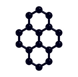
(a)

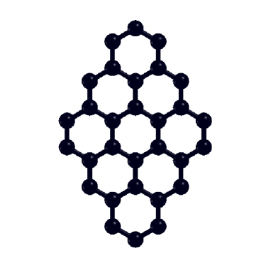
(b)

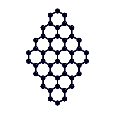
(c)

Figure 1: Schematic diagram of diamond shaped graphene quantum dots consisting of 16 atoms, 30 atoms and 48 atoms, respectively.

These calculations have been carried out by employing the PPP model Hamiltonian^{21; 22}, given by

$$H = - \sum_{i,j,\sigma}t_{ij}\left(c_{i\sigma}^{\dagger}c_{j\sigma}+c_{j\sigma}^{\dagger}c_{i\sigma}\right) + U\sum_{i}n_{i\uparrow}n_{i\downarrow} + \sum_{i<j}V_{ij}(n_{i}-1)(n_{j}-1)$$ (1)

where $c_{i\sigma}^{\dagger}($c${}_{i\sigma})$ creates (annihilates) a $\pi$ orbital of spin $\sigma$, localized on the ith carbon atom while the total number of electrons with spin $\sigma$ on atom $i$ is indicated by $n$${}_{i}=\sum_{\sigma}c_{i\sigma}^{\dagger}c_{i\sigma}$. The second and third terms in Eq. 1 denote the electron-electron repulsion terms, with the parameters $U$, and $V_{ij}$ representing the on-site, and the long-range Coulomb interactions, respectively. The matrix elements $t_{ij}$ depicts one-electron hops, which in our calculations, have been restricted to nearest neighbours, with the value $t{}_{0}$= 2.4 eV, consistent with our earlier calculations on conjugated polymers,^{23; 24; 25; 26; 27; 28; 29} and polyaromatic hydrocarbons.^{30; 31}

Parameterization of the Coulomb interactions is done according to the Ohno relationship ⁵⁴

$$V_{ij}=U/\kappa_{i,j}(1+0.6117R_{i,j}^{2})^{\nicefrac{{1}}{{2}}}$$ (2)

where $\kappa_{i,j}$ represents the dielectric constant of the system which replicates screening effects, $U$ as described above is the on-site electron-electron repulsion term, and $R_{i,j}$ is the distance (in Å) between the $i$th and $j$th carbon atoms. In the present work, we have done calculations adopting both “screened parameters”⁵⁵ with $U=8.0$ eV, $\kappa_{i,j}=2.0(i\neq j)$ and $\kappa_{i,i}=1.0$, as also the “standard parameters” with $U=11.13$ eV, and $\kappa_{i,j}=1.0$. We observe that our calculations employing the screened parameters, proposed by Chandross and Mazumdar,⁵⁵ are in better agreement with the experimental results, as compared to those performed using standard parameters, consistent with the trends observed in our earlier works as well.^{24; 27}

The first step of our calculations is to find the self-consistent solutions at the Restricted Hartree-Fock (RHF) level, employing the PPP Hamiltonian (cf. Eq. 1), using a code developed in our group.³⁴ These solutions, in which electrons occupy the lowest energy orbitals, comprise the HF ground state. This is followed by correlated calculations at the quadruple configuration interaction (QCI) level, or at the multi-reference singles-doubles configuration interaction (MRSDCI) level, depending upon the size of DQD. In the QCI approach, up to quadruple excitations from the HF ground state are considered, and, thus, it requires significant amount of computational resources. Therefore, QCI calculations can be performed only for small systems (in our case, for DQD-16). For larger DQDs, MRSDCI approach has been employed. In MRSDCI calculations, singly and doubly excited configurations from the reference configurations of the selected symmetry subspace are considered while generating the CI matrix.^{56; 57} Subsequently these CI wave functions are used to compute transition electric dipole matrix elements between various states, required for computing the optical absorption spectra. From the calculated spectra, important excited states giving rise to various peaks are identified, and the dominant reference configurations contributing to these excited states are included to enhance the new reference space. This procedure is iterated until the desired absorption spectrum converges to an acceptable tolerance. With the increasing sizes of the DQDs, the number of molecular orbitals of the DQD increases, leading to an increase in the size of the CI expansion. Therefore, to make calculations feasible, the frozen orbital approximation was adopted for DQD-48, with the lowest two occupied orbitals frozen, and highest two virtual orbitals deleted, so as to retain the particle-hole symmetry.

The formula employed for the calculation of the ground state optical absorption cross-section $\sigma(\omega)$, assumes a Lorentzian line shape

$$\sigma(\omega)=4\pi\alpha\underset{i}{\sum}\frac{\omega_{i0}\left|\left\langle i\left|\mathbf{\hat{e}.r}\right|0\right\rangle\right|^{2}\gamma}{\left(\omega_{i0}-\omega\right)^{2}+\gamma^{2}},$$ (3)

where $\omega$ denotes incident radiation frequency, $\hat{{\bf e}}$ denotes its polarization direction, ${\bf r}$ is the position operator, $\alpha$ is the fine structure constant, $0$ and $i$ denote, respectively, the ground and the excited states, $\omega_{i0}$ is the frequency difference between those states, and $\gamma$ is the absorption line-width.

III Results And Discussion

In this section, we present the results obtained from CI calculations for DQDs of varying sizes, ranging from DQD-16 to DQD-48. In order to acquaint the reader with the precision of our MRSDCI or QCI calculations, the sizes of the resultant CI matrix for different symmetries for the DQDs considered here are given in Table 1. QCI method was employed for carrying out calculations on ${}^{1}A_{g}$ and ${}^{1}B_{2u}$ manifolds of DQD-16, while rest of computations on DQD-16, DQD-30, and DQD-48, were carried out by adopting MRSDCI methodology. Sizes of the CI matrix indicate that electron-correlation effects were well accounted for in these calculations.

Table 1: Dimensions of CI matrices for DQDs of varying sizes, for various symmetry manifolds. QCI method was employed for carrying out calculations on ${}^{1}A_{g}$ and ${}^{1}B_{2u}$ manifolds of DQD-16, while for rest of the calculations MRSDCI method was used.

Number of atoms in DQD	Dimension of CI matrix
	${}^{1}A_{g}$	${}^{1}B_{2u}$	${}^{1}B_{3u}$
16	73857	126279	142992
30	215919	1564554	1359014
48	237030	5442399	4269236

III.1 Charge density distribution and optical gap

In this section we examine the evolution of the band gap, orbital energy levels, and the charge densities with the size of the DQD.

III.1.1 Charge Density

The charge density bubble-plots for the HOMO orbital obtained by employing the TB model and the PPP model for DQDs of varying sizes are presented in Fig. 2. The charge density of the LUMO orbital is same as that of the HOMO orbital because of the electron-hole symmetry, and hence has not been shown. The numbering scheme of atoms for the different DQDs considered is also presented.

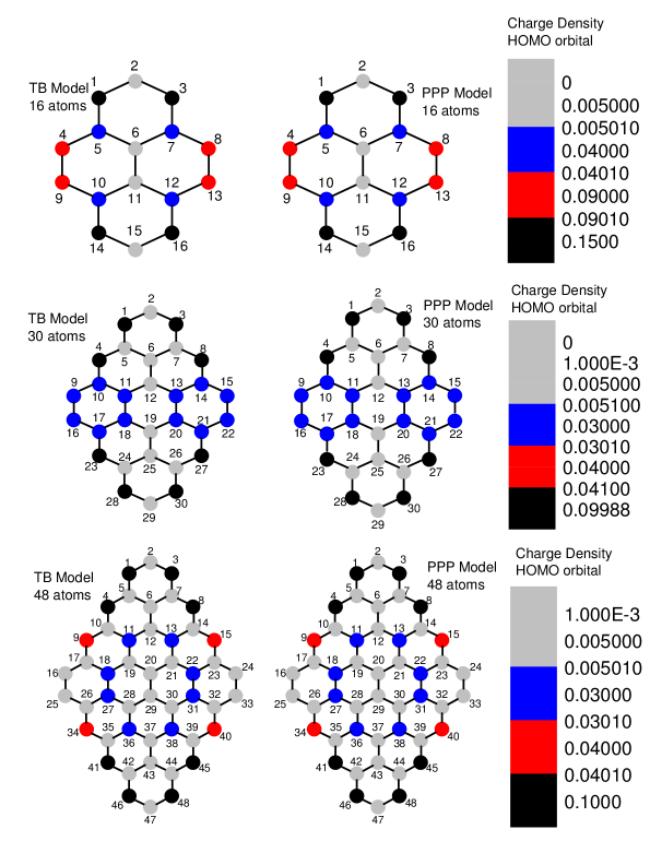
Figure 2: Charge density bubble plots of HOMO orbital obtained by employing TB and PPP models for DQDs of varying sizes. The numbering scheme of atoms for the different DQDs considered is also presented.

It is observed that in case of the smallest quantum dot DQD-16, the contribution from atomic sites 1, 3, 14 and 16 to the charge density of HOMO orbital is maximum. These atoms are at the projected corners of a purely zigzag edge as is evident from Fig. 2. The charge density contribution from the atomic sites 4, 8, 9, and 13, which are also at the edge of the diamond quantum dot, is less as compared to that of the atoms mentioned earlier. This can be attributed to the fact that these atoms give rise to an edge which exhibits both zigzag as well as armchair nature. With the increasing size of the quantum dot, the zigzag characteristic of the edge becomes more conspicuous, leading to increased contribution of the atoms located on the zigzag edges. This trend is obvious from the dominant contributions to the charge densities of the HOMO orbital by atoms 4, 8, 23 and 27 for DQD-30, and atoms 4, 8, 41 and 45, for DQD-48. From this it is evident that the HOMO-LUMO band-gap, and thus the optical properties of DQDs, can be tuned if suitable functional groups are attached to these atoms on the zigzag edges. This is in agreement with results obtained earlier for the case of graphene nano-ribbons (GNRs),⁵⁸ as well as triangular nanographenes.¹⁸

Looking at the energy-level diagrams of various DQDs presented in Fig. 3, unlike the case of triangular nanographenes with zigzag edges, one notices the absence of zero-energy states. It is also evident from the figure that the increasing size of DQDs leads to the reduction of the band gap, consistent with the gapless nature of infinite graphene.

Figure 3: Energy level plots for DQDs of varying sizes, calculated using the TB model.

III.1.2 Optical gap

In Table 2, we present the energy gap between the highest-occupied molecular orbital (HOMO), and the lowest-unoccupied molecular orbital (LUMO), for increasing sizes of DQDs obtained from the TB model, as well as from the PPP model, at the RHF level. Because the band gap is also the optical gap in DQDs, in the same table we also present the results of the optical gap of these systems obtained from our correlated electron CI calculations. We note the following trends in these results: (a) the gaps decrease with the increasing DQD size, irrespective of the Hamiltonian or the method used, (b) gaps obtained from the TB model are significantly smaller as compared to those obtained from other methods, (c) at the HF level standard parameter gaps are much larger than those obtained using screened parameter, (d) optical gaps at the CI level are significantly redshifted as compared to their HF values, in the standard parameter calculations. But, for the screened parameter calculations, these correlation-induced shifts are small, with the CI level gaps of DQD-16 and DQD-30 exhibiting slight redshifts, while that of DQD-48 exhibiting a small blueshift, and (e) at the CI level the gaps obtained using the two sets of PPP parameters are in good quantitative agreement with each other, suggesting the correctness of our correlated electron approach. This decrease of the gap with the increasing sizes observed for DQDs is in agreement with previous experimental and theoretical results obtained for graphene quantum dots of other shapes. ^{15; 17}

Table 2: HOMO-LUMO band gap for increasing size of DQDs obtained from the TB model and the PPP model. In case of PPP model, the gap is calculated both at the HF and CI level, using the standard (Std) as well as the screened (Scr) parameters. At the CI level, the gap is identified with the optical gap.

System	HOMO-LUMO gap (eV)	HOMO-LUMO gap (eV)		Optical gap (eV)
	(TB model)	(PPP-HF)		(PPP-CI)
		Scr	Std	Scr	Std
DQD-16	2.14	3.91	7.26	3.60	3.74
DQD-30	0.89	2.11	4.65	2.08	2.31
DQD-48	0.34	1.10	2.81	1.40	1.61

III.2 Linear Absorption spectrum

In this section, we first elucidate the salient features of the linear optical spectra of DQDs of varying sizes computed within the framework of the independent-electron TB model and PPP model at the HF level, which will allow us to gauge the influence of electron-correlation effects in the PPP model-based CI calculations, presented thereafter.

III.2.1 Calculations at the tight-binding and HF level

The absorption spectrum obtained from TB model and PPP model at HF level employing screened parameters (Fig. 4) exhibits the following characteristics:

1. The absorption spectrum is red-shifted with increase in size of the DQD, in agreement with quantum confinement effect. This red-shift is more pronounced at the PPP-HF level as compared to that obtained by the TB model. In addition, the absorption spectrum at the PPP-HF level is blue-shifted compared to the one computed using the TB model because it is well known that the HF theory overestimates energy gaps, as was also observed in earlier works. ^{59; 60}

2. The pattern of the absorption spectra at the PPP-HF level is similar to that obtained by the TB model. However, the absolute intensities of the peaks at the PPP-HF level are lesser as compared to those obtained by the TB model.

3. The first peak at the TB and PPP-HF level is always $y$-polarized, and corresponds to excitation of a single electron from the HOMO ($H$) orbital to the LUMO ($L$) orbital. This peak is also the most intense peak in the calculated spectra, which is in stark contrast with the experimental results obtained for pyrene and dibenzo[bc,kl]coronene.^{37; 43; 38; 39; 41; 61; 45; 42; 44; 40; 36}

4. With the increasing size of the DQDs, the intensity of the first peak increases enormously as compared to the other peaks in the absorption spectrum. For example, in DQD-30/DQD-48, the relative intensity of the peaks starting from the second one is much smaller as compared to DQD-16, irrespective of the Hamiltonian employed.

5. We also note that $x$-polarized peaks are degenerate, while $y$-polarized peaks exhibit no degeneracy. For example, in case of DQD-16, the second peak is $x$-polarized and is due to degenerate excitations $|H-1\rightarrow L\rangle$ and $|H\rightarrow L+1\rangle$, while the third peak is $y$-polarized, and is due to nondegenerate excitation $|H-1\rightarrow L+1\rangle$.

Figure 4: Optical absorption spectrum of DQD-16, DQD-30, and DQD-48, calculated using the tight binding model and PPP model at HF level employing screened parameters. The spectrum has been broadened with a uniform line width of 0.1 eV.

Table 3: Comparison of locations of experimentally measured linear absorption peaks of pyrene and dibenzo[bc,kl]coronene with our PPP-CI results for DQD-16 and DQD-30, respectively. Computed values of the excited state energies for DQD-48 are also presented. DF and MI, respectively, denote dipole forbidden state, and most intense peak. Theoretical results of other authors are also presented for comparison. All energies are in eV units.

System	Symmetry	Experimental Values	Theory	This work
			(Other)
				Scr	Std
DQD-16	$B$3u (DF)	3.34,37 3.33,42	3.33,50 3.83,42 3.7551	2.82	3.09
	$B$2u	3.70,37 3.69,39; 38 3.71,40 3.80,41	3.35,52 3.53,50 3.93,42 3.6951	3.60	3.74
	(optical gap)	3.75,43 3.79,42 3.8344
	$B$3u	4.55,39; 40; 37 4.62,42	4.10,52 4.70,50 5.2642	4.37	4.94
		4.67,41; 44 4.60,43
	$B$2u	5.15,37 5.12,39; 38 5.17,40 5.29,42	5.00,52 5.36 ,50 5.60 42	5.37	5.44
		5.34,41; 44 5.35,36 5.2243
	$B$2u	6.32,37 6.0742	5.80,52 5.96,50 6.6642	6.22	6.44
	$B$3u	6.4242	6.04,50 6.35 ,52 6.9642	6.38	6.96
	$B$2u, $B$3u	7.0242	6.45,50 7.39,52 7.5142	6.88, 6.87	7.29, 7.33
	$B$2u(MI)	5.15,37 5.12,39; 38 5.17,40 5.29,42	6.35,52 5.36 ,50 5.60 42	5.37	6.44
		5.34,41; 44 5.35,36 5.2243
DQD-30	$B$2u	2.5545	2.1053; 35	2.08	2.31
	(optical gap)
	$B$3u (DF)			2.25	2.43
	$B$3u	3.6145	3.5553; 35	3.45	3.83
	$B$3u(MI)	6.2061	5.9053; 35	6.28	5.10
DQD-48	$B$3u (DF)			1.38	1.52
	$B$2u			1.40	1.61
	(optical gap)
	$B$2u(MI)			2.19	5.54

III.2.2 Correlated-electron calculations

We discuss the general features of the optical absorption spectra obtained from the CI calculations, followed by a more detailed examination of individual DQDs.

One observes the following general trends upon examining the absorption spectra calculated by the PPP-CI approach presented in Figs. 5—7, and the quantitative information about various excited states detailed in Tables 4—10 of the Appendix:

1. In agreement with the TB results, the absorption spectrum is red-shifted with the increasing size of the DQD.

2. The spectra obtained from screened parameters is red-shifted as compared to that obtained from standard parameters. Furthermore, for the case of DQD-16^{37; 38; 43; 39; 42; 44; 40; 41; 36} and DQD-30^{61; 45}, screened parameter results are in overall better agreement with the experimental data (cf. Table 3), as compared to the standard parameter ones.

3. The first peak in the spectrum of the DQDs is always due to the absorption of a $y$-polarized photon, causing a transition from their ground state ($1^{1}A_{g}$), to the $1^{1}B_{2u}$ excited state, and denotes the optical gap. The wave function of the $1^{1}B_{2u}$ state for all the DQDs is dominated by the $|H\rightarrow L\rangle$ excitation, in agreement with the results of the TB model. However, a quantitative analysis of the optical gap indicates that its value obtained from the TB model is much less compared to the value obtained from the PPP-CI approach. For the cases of DQD-16^{37; 38; 43; 39; 42; 44; 40; 41; 36} and DQD-30,^{61; 45} for which the experimental results are available, again PPP-CI value of the gap is in much better agreement with experimental results, than the TB model value. Therefore, we hope that similar experiments can be performed on DQD-48 in the future, so that our predicted PPP-CI values of optical gaps can be tested.

4. The intensity of the first peak is lesser as compared to the intensity of other higher energy peak(s) in the spectrum, in contrast to the predictions of the TB model, and in agreement with the experimental results for pyrene,^{37; 38; 43; 39; 42; 44; 40; 41; 36} and dibenzo[bc,kl]coronene.^{61; 45}

5. The calculated position of the first peak in the PPP-CI absorption spectrum is weakly dependent on the choice of the Coulomb parameters in the PPP model (standard or screened). However, higher energy peaks, and the character of the many-particle wave functions contributing to them, do depend significantly upon the choice of Coulomb parameters. In particular, the position of the most intense peak is drastically dependent upon the choice of the Coulomb parameters in the PPP-CI calculations. Thus, we conclude that the position of the most intense peak is strongly dependent on the strength of the Coulomb interactions in theses systems.

6. The optical transition to the first excited state of $B_{3u}$ symmetry is dipole forbidden within the PPP model, on account of the particle-hole symmetry due to the use of the nearest-neighbour hopping approximation. However, this symmetry is approximate in the real systems, and hence the transition to this state is experimentally observed as a weak peak. Our PPP-CI calculations predict this state to lie below the optical gap for DQD-16 and DQD-48, but above it for DQD-30. (cf. Tables 4, 5, 6, 7, 8 and 10). Our prediction is in agreement with the experiments for the case of DQD-16 when compared with the data for pyrene (cf. Table 3 ), however, no experimental results for this state are available for the larger DQDs.

7. Wave functions of higher energy states derive significant contributions from double and higher level excitations, signaling the importance of electron correlation effects.

DQD-16

Figure 5 presents the computed linear absorption spectrum for DQD-16, obtained by employing standard as well as screened parameters, while Tables 4 and 5, of the Appendix, present the detailed quantitative data corresponding to various peaks in the computed spectra, and the excited states contributing to them. Our theoretical results have been compared with the experimental optical absorption data of pyrene (C₁₆H₁₀), which is nothing but hydrogen saturated DQD-16. Because we have employed PPP model parameters used to describe the optical properties of aromatic hydrocarbons, the comparison between DQD-16 and pyrene is most appropriate. A number of theoretical^{50; 42; 51; 52} and experimental studies^{37; 38; 43; 39; 42; 44; 40; 41; 36} of optical absorption in pyrene have been carried out in the past, and our calculated excited state energies are found to to be in very good agreement with the results obtained earlier (cf. Table 3 ).

The first peak in the experimentally obtained absorption spectrum of pyrene is a weak one located around 3.34 eV,³⁷ and corresponds to the dipole forbidden $B_{3u}$ state in our calculations, mentioned earlier. Our standard parameter value of 3.09 eV for the excitation energy of this state is in good agreement with the experimental value, while the screened parameter value of 2.82 eV underestimates it. The location of the second peak in the experimental spectrum (3.69-3.83 eV), which also defines the optical gap, is in excellent agreement both with our standard and screened parameter PPP-CI values of the optical gap, computed at 3.74 eV, and 3.60 eV, respectively. This peak is $y$-polarized and corresponds to $1B_{2u}$ state. The optical transition to the fourth excited state gives rise to the most intense peak experimentally observed to be in the range 5.15–5.35 eV. This result is in excellent agreement with our PPP-CI value 5.37 eV, obtained using the screened parameters. As a matter of fact, it is obvious from Table 3, that the agreement between the dipole-allowed states obtained from our screened-parameter based PPP-CI calculations, and the experimental measurements of Becker et al.³⁷ and Gudipati et al.⁴² is quite remarkable both for peak locations, and the symmetry assignments, all the way up to 7 eV. On the other hand, the PPP-CI results obtained using standard parameters, as also the earlier results obtained by Malloci et al.,⁵² predict that transition to the fifth excited state gives rise to the most intense peak. Thus, we conclude that, on the whole, the PPP-CI results calculated using the screened parameters are in better agreement with the experimental values than those computed using the standard parameters (cf. Table 3). Screened parameter based calculations also predict that the wave functions of the excited states of the first five peaks (I–V) are dominated by single excitations (cf. Table 5). We also note that the TB model predicts the peak corresponding to the optical gap as the most intense one, located at 2.14 eV, which is far away from the experimentally obtained value both in terms of peak location, and relative intensity. Therefore, we infer that the inclusion of electron correlation effects is essential for the correct quantitative description of the optical properties of graphene quantum dots.

Figure 5: Computed linear optical absorption spectrum for 16 atoms DQD, obtained by employing screened as well as standard parameters. In both the cases, the spectrum has been broadened with a uniform line-width of 0.1 eV.

DQD-30 and DQD-48

In Figs. 6 and 7, we present the computed linear absorption spectra for DQD-30 and DQD-48, respectively. Information related to the energies, transition dipoles, and many-particle wave functions of excited states contributing to various absorption peaks for DQD-30 are presented in Tables 6 and 7 of the Appendix.

Figure 6: Computed linear optical absorption spectrum for 30 atoms DQD, obtained by employing screened as well as standard parameters. In both the cases, the spectrum has been broadened with a uniform line-width of 0.1 eV.

As far as DQD-30 is concerned, our computed absorption spectrum has been compared with the experimental data of dibenzo[bc,kl]coronene (C₃₀H₁₄).⁴⁵ The experimental UV spectrum obtained by Clar and Schmidt,⁴⁵ exhibits peaks at 2.55 eV and 3.61 eV. The position of the first peak at 2.55 eV is in good agreement with the computed value of optical gap at 2.08 eV (2.31 eV) (cf. Table 3) obtained using screened (standard) parameters in the PPP-CI model. This peak is $y$-polarized, and corresponds to the $1B_{2u}$ state. The first excited state of $B_{3u}$ symmetry is dipole forbidden due to the particle-hole symmetry, and lies above the optical gap. Its energy is 2.25 eV (2.43 eV) obtained using screened (standard) parameters and is dominated by the $|H-2\rightarrow L\rangle+c.c.$ excitation. In addition, the experimental peak at 3.61 eV agrees extremely well with the screened parameter $x-$polarized peak at 3.45 eV. This peak corresponds to a $B_{3u}$ state, whose wave function is dominated by the $|H-2\rightarrow L\rangle-c.c$ excitation. Thus, same excitations contribute to the wave functions of the first dipole-forbidden and dipole-allowed $B_{3u}$ states, it is just that their relative signs are opposite due to the orthogonality constraint. Further, the most intense peak of the experimental spectrum is situated at around 6.20 eV,⁶¹ which is in excellent agreement with the computed screened parameter value of the most intense peak at 6.28 eV. This peak also corresponds to a $B_{3u}$ state whose wave function consists of singly as well as doubly excited configurations (cf. Table 7). On the other hand, our standard parameter calculations predict the most intense absorption peak at 5.10 eV corresponding to a $B_{2u}$ state, whose wave function consists mainly of single excitations, dominated by the configuration $|H-2\rightarrow L+2\rangle$ (cf. Table 6). Thus, our computations imply that screened parameter values are in better overall agreement with the experimental results than standard parameter values, and TB model predictions. While wave functions of the excited states corresponding to various peaks are dominated by single excitations, however, several states also derive significant contributions from the double excitations, hinting at the importance of electron correlation effects.

In case of DQD-48, because of comparatively larger number of electrons in the system, the size of the MRSDCI calculations became excessively large. Therefore, we froze two lowest lying occupied orbitals, and deleted their particle-hole counterpart virtual orbitals which were highest in energy. With this approximation in place, the CI problem reduced to that of 44 electrons, distributed over 22 occupied, and as many virtual orbitals, rendering the calculation tractable. In order to benchmark this procedure, we also adopted the same methodology for DQD-30, and present the results of the calculations performed using screened parameters in Fig. 8 of the Appendix. It is observed that all the features of the optical spectra are preserved even after freezing the orbitals. However, the frozen spectrum is slightly blue-shifted as compared to the unfrozen one, with the corresponding changes being numerically acceptable. Next, we discuss our results for DQD-48 presented in Fig. 7, and Tables 8, 9, and 10.

We find that the first excited state of DQD-48 is a dipole forbidden $B_{3u}$ state, just as in the case of DQD-16, and is located at 1.38 eV (1.52 eV) as per our screened (standard) parameter calculations. Both the calculations predict it to be lower than the first dipole allowed state $1B_{2u}$, although the energy difference is much smaller as compared to the case of DQD-16. The wave function of this $B_{3u}$ state is dominated by the double excitation $|H\rightarrow L+1;H\rightarrow L\rangle+c.c.$, and it will be of considerable interest if the future experiments on DQD-48 are able to locate this state relative to the optical gap. The first dipole-allowed peak in the absorption spectrum of DQD-48, corresponding to the $1B_{2u}$ state of the spectrum as in case of smaller DQDs, is computed at 1.61 eV (1.40 eV) based upon standard (screened) parameter based PPP-CI calculations. The wave function of this state is dominated by the $|H\rightarrow L\rangle$ excitation as in case of smaller dots, but it also derives significant contribution from the $|H-1\rightarrow L+1\rangle$ configuration. The most intense peak of the absorption spectrum computed with the screened parameter is peak II corresponding to the $2B_{2u}$ state located at 2.19 eV, with the wave function dominated by the $|H-1\rightarrow L+1\rangle$ configuration, but also with a significant contribution from a triply excited configuration. On the other hand, standard parameter calculations predict peak XII to be the most intense one, which is due to a high-energy $B_{2u}$ state at 5.54 eV, with the wave function dominated by several configurations. Such a large difference in the locations of the most intense peak predicted by standard and screened parameter calculations, can be easily tested in experiments. As far as general comparison between the standard and screened parameter calculations is concerned, besides the red shift of the screened parameter results compared to the standard ones, we find that only the first two peaks of the computed spectra have excited state wave functions which are qualitatively similar. We also note that compared to the two smaller DQDs discussed earlier, DQD-48 excited states exhibit significantly more contribution from doubly excited configurations. This trend implies higher contribution of electron-correlation effects in DQD-48.

Figure 7: Computed linear absorption spectra (with a line-width of 0.1 eV) for 48 atoms DQD, obtained by employing standard as well as screened parameters

IV Conclusions

In this work, very large scale correlated calculations employing the PPP Hamiltonian were carried out on diamond shaped graphene quantum dots of increasing sizes, namely, DQD-16, DQD-30, and DQD-48, and their optical as well as electronic properties were computed. Calculated linear optical absorption spectra of DQD-16 and DQD-30 were found to be in very good agreement with the experimental data of pyrene (C₁₆H₁₀) and dibenzo[bc,kl]coronene (C₃₀H₁₄), which are their respective structural analogs with hydrogen passivated edges, thus justifying the essential correctness of our methodology. Some of the important conclusions we can draw from our correlated-electron calculations are: (i) the first peak corresponding to the optical gap is not the most intense, in contrast with the predictions of the tight-binding model, (ii) with the increasing size of the quantum dot, the absorption spectrum exhibits a red shift, (iii) the optical transition to the first excited state of $B_{3u}$ symmetry is dipole forbidden and it lies below the optical gap for DQD-16 and DQD-48, (iv) optical properties of the dots are sensitive to the projected corners of the system, therefore, they can be tuned by attaching suitable functional groups there. Thus, we hope that our work will spur further experimental activity in this field, so that our predictions on the excited states of DQD-48 can be tested in future experiments. Furthermore, recently Müllen and coworkers have stabilized graphene quantum dots with chlorine passivated edges.⁵⁸ Therefore, it will be of interest if chlorine passivated DQDs can be synthesized and their optical properties measured, so as to investigate the influence of the nature of edge passivation on the electro-optical properties of graphene nanostructures.

In this work, we restricted ourselves to the study of linear optical properties of these quantum dots, but it will be quite interesting also to study the nonlinear optical response of these systems such as two-photon absorption, third harmonic generation, and photoinduced absorption. Calculations along those directions are underway in our group, and the results will be submitted for publication in future.

Appendix A Influence of orbital freezing and deletion on the optical absorption spectrum of DQD-30

In order to benchmark our orbital freezing and deletion approach aimed at reducing the size of the CI calculations, in the figure below we present the results of optical absorption spectra of DQD-30 computed using all the electrons and orbitals, and by freezing (deleting) two lowest (highest) occupied (virtual) orbitals. Apart from a slight blue shift in the frozen orbital calculation, computed spectra are quite similar.

Figure 8: Computed absorption spectrum (with a line-width of 0.1 eV) for 30 atoms DQD, obtained by freezing orbitals (dotted line) and without freezing orbitals (bold line).

Appendix B Calculated Energies, Wave Functions, and Transition Dipole Moments Of The Excited States Contributing To The Linear Absorption Spectra

Following tables represent the excitation energies, dominant many-body wave-functions, and transition dipole matrix elements of excited states with respect to the ground state (1¹A_g). The coefficient of charge conjugate of a given singly excited configuration is abbreviated as ’c.c.’, while the sign (+/-) preceding ’c.c.’ indicates that the two coefficients have (same/opposite) signs. For the doubly excited, and the higher order configurations, no +/- sign precedes c.c. because more than one charge-conjugate counterparts are possible, each with its own sign. Label DF associated with a peak implies that the excited state in question is dipole forbidden.

Table 4: Excited states giving rise to the peaks in the linear absorption spectrum of 16 atoms DQD, computed employing the QCI ($B_{2u}$ states) and MRSDCI ($B_{3u}$ states) approaches, along with the standard parameters in the PPP model Hamiltonian.

Peak	State	E (eV)	Transition Dipole (Å)	Dominant Configurations
$DF$	$1^{1}B\textrm{${}_{3u}$}$	$3.09$	$0$	$|H\rightarrow L+1\rangle$$-c.c.(0.5919)$
				$|H-4\rightarrow L+3\rangle$$-c.c.(0.1244)$
$I_{y}$	$1^{1}B\textrm{${}_{2u}$}$	$3.74$	$1.137$	$|H\rightarrow L\rangle$$(0.8606)$
				$|H-1\rightarrow L+1\rangle$$(0.2855)$
$II_{x}$	$2^{1}B\textrm{${}_{3u}$}$	$4.94$	$1.094$	$|H-1\rightarrow L\rangle$$+c.c.(0.5897)$
				$|H\rightarrow L+1;H-3\rightarrow L\rangle$$c.c.(0.1440)$
				$|H-2\rightarrow L+3\rangle$$-c.c.(0.1377)$
$III_{y}$	$3^{1}B\textrm{${}_{2u}$}$	$5.44$	$1.117$	$|H-1\rightarrow L+1\rangle$$(0.7593)$
				$|H-2\rightarrow L+2\rangle$$(0.3370)$
$IV_{y}$	$5^{1}B\textrm{${}_{2u}$}$	$6.44$	$1.482$	$|H-2\rightarrow L+2\rangle$$(0.7125)$
				$|H-1\rightarrow L+1\rangle$$(0.3400)$
$V_{x}$	$8^{1}B\textrm{${}_{3u}$}$	$6.96$	$1.169$	$|H-3\rightarrow L+2\rangle$$-c.c.(0.4736)$
				$|H\rightarrow L+2;H\rightarrow L\rangle$$+c.c.(0.3047)$
$VI_{x\&y}$	$10B\textrm{${}_{2u}$}$	$7.29$	$0.255$	$|H-2\rightarrow L+4\rangle$$-c.c.(0.4346)$
				$|H-3\rightarrow L+3\rangle$$(0.3309)$
	$9^{1}B\textrm{${}_{3u}$}$	$7.33$	$0.459$	$|H\rightarrow L+6\rangle$$-c.c.(0.4957)$
				$|H-1\rightarrow L;H-3\rightarrow L\rangle$$-c.c.(0.1993)$

Table 5: Excited states giving rise to the peaks in the linear absorption spectrum of 16 atoms DQD, computed employing the QCI ($B_{2u}$ states) and MRSDCI ($B_{3u}$ states) approaches, along with the screened parameters in the PPP model Hamiltonian.

Peak	State	E (eV)	Transition Dipole (Å)	Dominant Configurations
$DF$	$1^{1}B\textrm{${}_{3u}$}$	$2.82$	$0$.000	$|H\rightarrow L+1\rangle$$-c.c.(0.5730)$
				$|H\rightarrow L+4;H\rightarrow L\rangle$$+c.c.(0.1090)$
$I_{y}$	$1^{1}B\textrm{${}_{2u}$}$	$3.60$	$1.477$	$|H\rightarrow L\rangle$$(0.8802)$
$II_{x}$	$2^{1}B\textrm{${}_{3u}$}$	$4.37$	$1.272$	$|H-1\rightarrow L\rangle$$+c.c.$ $(0.6042)$
				$|H\rightarrow L+1;H-3\rightarrow L\rangle$$c.c.$ $(0.0820)$
				$|H-3\rightarrow L+2\rangle$$+c.c.$ $(0.0818)$
$III_{y}$	$3^{1}B\textrm{${}_{2u}$}$	$5.37$	$1.424$	$|H-1\rightarrow L+1\rangle$$(0.8596)$
				$|H-1\rightarrow L+1;H\rightarrow L;H\rightarrow L\rangle$$(0.1113)$
$IV_{y}$	$5^{1}B\textrm{${}_{2u}$}$	$6.22$	$0.746$	$|H-2\rightarrow L+2\rangle$$(0.6716)$
				$|H\rightarrow L+5\rangle$$-c.c.$ $(0.3187)$
$V_{x}$	$8^{1}B\textrm{${}_{3u}$}$	$6.38$	$1.205$	$|H-2\rightarrow L+3\rangle$$+c.c.(0.5243)$
				$|H\rightarrow L+2;H\rightarrow L\rangle$$+c.c.(0.2700)$
$VI_{x\&y}$	$9^{1}B\textrm{${}_{3u}$}$	$6.87$	$0.049$	$|H\rightarrow L+6\rangle$$-$$c.c.(0.3507)$
				$|H-4\rightarrow L+3\rangle$$-c.c.(0.2767)$
	$10^{1}B\textrm{${}_{2u}$}$	$6.88$	$0.396$	$|H-3\rightarrow L+3\rangle$$(0.3983)$
				$|H-2\rightarrow L+4\rangle$$-c.c.(0.2996)$
				$|H\rightarrow L+5\rangle$$-c.c.(0.2671)$
$VII_{x}$	$10^{1}B\textrm{${}_{3u}$}$	$7.03$	$0.510$	$|H-2\rightarrow L;H\rightarrow L\rangle$$+c.c.(0.3680)$
				$|H-6\rightarrow L\rangle$$-c.c.(0.2715)$
$VIII_{x}$	$13^{1}B\textrm{${}_{3u}$}$	$7.33$	$0.402$	$|H-1\rightarrow L+5\rangle$$-c.c.(0.4156)$
				$|H-3\rightarrow L+4\rangle$$-c.c.(0.2626)$

Table 6: Excited states giving rise to the peaks in the linear absorption spectrum of DQD-30, computed employing the MRSDCI approach along with standard parameters in the PPP model Hamiltonian.

Peak	State	E (eV)	Transition Dipole (Å)	Dominant Configurations
$I_{y}$	$1^{1}B\textrm{${}_{2u}$}$	$2.31$	$1.748$	$|H\rightarrow L\rangle$$(0.8223)$
				$|H-1\rightarrow L+1\rangle$$(0.1632)$
$DF$	$1^{1}B\textrm{${}_{3u}$}$	$2.43$	$0$.000	$|H-2\rightarrow L\rangle$$-c.c.(0.4970)$
				$|H\rightarrow L+1;H\rightarrow L\rangle$$+c.c.(0.2365)$
$II_{x\&y}$	$3^{1}B\textrm{${}_{3u}$}$	$3.83$	$1.048$	$|H-2\rightarrow L\rangle$$+c.c.(0.5432)$
				$|H-5\rightarrow L;H\rightarrow L\rangle+$$c.c.(0.1563)$
	$4^{1}B\textrm{${}_{2u}$}$	$3.85$	$1.065$	$|H-1\rightarrow L+1\rangle$$(0.4738)$
				$|H-4\rightarrow L\rangle$$-c.c.$ $(0.4659)$
				$|H-1\rightarrow L+1;H\rightarrow L;H\rightarrow L\rangle$$(0.1507)$
$III_{y}$	$5^{1}B\textrm{${}_{2u}$}$	$4.20$	$0.892$	$|H-1\rightarrow L+1\rangle$$(0.5236)$
				$|H-4\rightarrow L\rangle$$-c.c.$ $(0.3332)$
$IV_{x}$	$8^{1}B\textrm{${}_{3u}$}$	$4.74$	$1.047$	$|H-1\rightarrow L;H\rightarrow L\rangle$$-c.c.(0.3713)$
				$|H-1\rightarrow L+3\rangle$$+c.c.(0.2959)$
$V_{y}$	$9^{1}B\textrm{${}_{2u}$}$	$5.10$	$1.563$	$|H-2\rightarrow L+2\rangle$$(0.5107)$
				$|H-7\rightarrow L\rangle$$-c.c.(0.2136)$
				$|H-3\rightarrow L;H\rightarrow L\rangle$$-c.c.(0.2088)$
				$|H-1\rightarrow L+1\rangle$$(0.2046)$
$VI_{x\&y}$	$14^{1}B\textrm{${}_{3u}$}$	$5.66$	$0.480$	$|H-3\rightarrow L+1\rangle$$+c.c.(0.3604)$
				$|H\rightarrow L+1;H\rightarrow L\rangle$$-c.c.(0.2197)$
				$|H-8\rightarrow L\rangle+$$c.c.(0.1840)$
	$15^{1}B\textrm{${}_{2u}$}$	$5.70$	$1.017$	$|H-2\rightarrow L+2\rangle$$(0.3796)$
				$|H-3\rightarrow L+3\rangle$$(0.3475)$
				$|H-1\rightarrow L;H-2\rightarrow L\rangle$$-c.c.(0.2148)$
$VII_{y}$	$20^{1}B\textrm{${}_{2u}$}$	$6.22$	$1.113$	$|H-4\rightarrow L+4\rangle$$(0.3458)$
				$|H-1\rightarrow L+1;H\rightarrow L;H\rightarrow L\rangle$$(0.2964)$

Table 7: Excited states giving rise to the peaks in the linear absorption spectrum of DQD-30, computed employing the MRSDCI approach along with screened parameters in the PPP model Hamiltonian.

Peak	State	E (eV)	Transition Dipole (Å)	Dominant Configurations
$I_{y}$	$1^{1}B\textrm{${}_{2u}$}$	$2.08$	$2.036$	$|H\rightarrow L\rangle$$(0.8387)$
				$|H-1\rightarrow L+1\rangle$$(0.1389)$
$DF$	$1^{1}B\textrm{${}_{3u}$}$	$2.25$	$0.000$	$|H-2\rightarrow L\rangle$$+c.c.(0.4918)$
				$|H\rightarrow L+1;H\rightarrow L\rangle$$-c.c.(0.2691)$
$II_{x}$	$3^{1}B\textrm{${}_{3u}$}$	$3.45$	$1.443$	$|H-2\rightarrow L\rangle-$$c.c.(0.5819)$
$III_{y}$	$4^{1}B\textrm{${}_{2u}$}$	$3.71$	$1.654$	$|H-1\rightarrow L+1\rangle$$(0.7000)$
				$|H-4\rightarrow L\rangle+$$c.c.(0.2500)$
				$|H-1\rightarrow L+1;H\rightarrow L;H\rightarrow L\rangle$$(0.2466)$
$IV_{x}$	$7^{1}B\textrm{${}_{3u}$}$	$4.23$	$0.594$	$|H-6\rightarrow L\rangle-$$c.c.(0.4901)$
				$|H-1\rightarrow L;H\rightarrow L\rangle+$$c.c.(0.2549)$
$V_{x\&y}$	$11^{1}B\textrm{${}_{3u}$}$	$4.90$	$1.119$	$|H-3\rightarrow L+1\rangle+$$c.c.(0.5083)$
				$|H-5\rightarrow L;H\rightarrow L\rangle+$$c.c.(0.1442)$
				$|H-7\rightarrow L+1;H\rightarrow L\rangle$$-$$c.c.(0.1350)$
	$10^{1}B\textrm{${}_{2u}$}$	$4.83$	$1.221$	$|H-2\rightarrow L+2\rangle$$(0.5634)$
				$|H-2\rightarrow L+1;H\rightarrow L\rangle$$c.c.(0.2359)$
				$|H-1\rightarrow L+5\rangle$$+c.c.(0.2065)$
$VI_{y}$	$15^{1}B\textrm{${}_{2u}$}$	$5.32$	$0.632$	$|H\rightarrow L+3;H\rightarrow L\rangle+$$c.c.(0.3245)$
				$|H-7\rightarrow L\rangle-$$c.c.(0.3079)$
				$|H-1\rightarrow L;H-2\rightarrow L\rangle-$$c.c.(0.2057)$
$VII_{x}$	$20^{1}B\textrm{${}_{3u}$}$	$5.69$	$0.431$	$|H-2\rightarrow L+4\rangle-$$c.c.(0.4019)$
				$|H-1\rightarrow L+1;H\rightarrow L+1\rangle+$$c.c.(0.2542)$
				$|H-1\rightarrow L;H-4\rightarrow L\rangle+$$c.c.(0.2371)$
$VIII_{x}$	$23^{1}B\textrm{${}_{3u}$}$	$5.97$	$0.498$	$|H-7\rightarrow L+2\rangle+$$c.c.(0.3404)$
				$|H\rightarrow L+2;H-3\rightarrow L\rangle$$c.c.(0.3106)$
$IX_{x}$	$29^{1}B\textrm{${}_{3u}$}$	$6.28$	$1.063$	$|H-3\rightarrow L+5\rangle+$$c.c.(0.3091)$
				$|H-6\rightarrow L+4\rangle-$$c.c.(0.2390)$

Table 8: Excited states giving rise to the peaks $I_{y}$ to $VII_{y}$ in the linear absorption spectrum of DQD-48, computed employing the MRSDCI approach along with standard parameters in the PPP model Hamiltonian.

Peak	State	E (eV)	Transition Dipole (Å)	Dominant Configurations
$DF$	$1^{1}B\textrm{${}_{3u}$}$	$1.52$	$0$.000	$|H\rightarrow L+1;H\rightarrow L\rangle-$$c.c.(0.4873)$
				$|H-4\rightarrow L\rangle+$$c.c.(0.2313)$
$I_{y}$	$1^{1}B\textrm{${}_{2u}$}$	$1.61$	$1.402$	$|H\rightarrow L\rangle$$(0.7467)$
				$|H-1\rightarrow L+1\rangle$$(0.3061)$
$II_{y}$	$3^{1}B\textrm{${}_{2u}$}$	$2.57$	$2.180$	$|H-1\rightarrow L+1\rangle$$(0.5160)$
				$|H-1\rightarrow L+1;H\rightarrow L;H\rightarrow L\rangle$$(0.4413)$
				$|H-2\rightarrow L\rangle$$+c.c.(0.2739)$
$III_{x}$	$3^{1}B\textrm{${}_{3u}$}$	$2.76$	$1.043$	$|H\rightarrow L+1;H\rightarrow L\rangle+$$c.c.(0.4903)$
				$|H\rightarrow L+5\rangle-$$c.c.(0.2202)$
				$|H\rightarrow L+1;H-1\rightarrow L+1\rangle+$$c.c.(0.1449)$
$IV_{y}$	$5^{1}B\textrm{${}_{2u}$}$	$2.88$	$1.067$	$|H-2\rightarrow L\rangle+$$c.c.(0.4765)$
				$|H-1\rightarrow L+1\rangle$$(0.2689)$
				$|H-1\rightarrow L+1;H\rightarrow L;H\rightarrow L\rangle$$(0.2549)$
$V_{x}$	$6^{1}B\textrm{${}_{3u}$}$	$3.38$	$0.933$	$|H-4\rightarrow L\rangle-$$c.c.(0.4874)$
				$|H-6\rightarrow L;H\rightarrow L\rangle+$$c.c.(0.2237)$
				$|H-3\rightarrow L+1\rangle-$$c.c.(0.1679)$
$VI_{y}$	$6^{1}B\textrm{${}_{2u}$}$	$3.66$	$1.727$	$|H-3\rightarrow L;H\rightarrow L\rangle$$(0.3471)$
				$|H-1\rightarrow L+1\rangle$$(0.2908)$
$VII_{y}$	$10^{1}B\textrm{${}_{2u}$}$	$4.16$	$0.939$	$|H-2\rightarrow L+2\rangle$$(0.3609)$
				$|H-1\rightarrow L+7\rangle+$$c.c.(0.3331)$

Table 9: Excited states giving rise to the peaks $VIII_{y}$ to $XII_{y}$ in the linear absorption spectrum of DQD-48, computed employing the MRSDCI approach along with standard parameters in the PPP model Hamiltonian.

Peak	State	E (eV)	Transition Dipole (Å)	Dominant Configurations
$VIII_{y}$	$13^{1}B\textrm{${}_{2u}$}$	$4.37$	$0.596$	$|H-4\rightarrow L+1;H\rightarrow L\rangle$$c.c.(0.3129)$
				$|H-4\rightarrow L+4\rangle$$(0.2685)$
				$|H-1\rightarrow L;H-4\rightarrow L\rangle-$$c.c.(0.2191)$
$IX_{x\&y}$	$13^{1}B\textrm{${}_{3u}$}$	$4.59$	$0.839$	$|H-3\rightarrow L+1\rangle-$$c.c.(0.4035)$
				$|H-8\rightarrow L;H\rightarrow L+1\rangle$$c.c.(0.1534)$
				$|H\rightarrow L+5\rangle-$$c.c.(0.1371)$
	$18^{1}B\textrm{${}_{2u}$}$	$4.65$	$0.231$	$|H\rightarrow L+4;H\rightarrow L+1\rangle-$$c.c.(0.2687)$
				$|H-6\rightarrow L+1\rangle+$$c.c.(0.2665)$
				$|H\rightarrow L+9;H\rightarrow L\rangle+$$c.c.(0.2156)$
$X_{y}$	$20^{1}B\textrm{${}_{2u}$}$	$4.80$	$0.347$	$|H-4\rightarrow L+1;H\rightarrow L\rangle$$c.c.(0.2900)$
				$|H-1\rightarrow L+5;H\rightarrow L\rangle$$c.c.(0.1942)$
				$|H-2\rightarrow L+2\rangle$$(0.1894)$
$XI_{x\&y}$	$20^{1}B\textrm{${}_{3u}$}$	$4.96$	$0.237$	$|H-9\rightarrow L+1\rangle+$$c.c.(0.4364)$
				$|H-8\rightarrow L;H\rightarrow L+1\rangle$$c.c.(0.1441)$
				$|H-10\rightarrow L;H\rightarrow L\rangle$$-c.c.(0.1418)$
	$23^{1}B\textrm{${}_{2u}$}$	$4.98$	$0.634$	$|H-2\rightarrow L+2\rangle$$(0.2775)$
				$|H-1\rightarrow L+5;H\rightarrow L\rangle$$c.c.(0.2171)$
				$|H-4\rightarrow L+1;H\rightarrow L\rangle$$c.c.(0.2162)$
$XII_{y}$	$33{}^{1}B\textrm{${}_{2u}$}$	$5.54$	$1.183$	$|H-4\rightarrow L+4\rangle$$(0.2954)$
				$|H-13\rightarrow L\rangle+$$c.c.(0.2185)$
				$|H-1\rightarrow L+1;H\rightarrow L+3\rangle$$c.c.(0.2098)$

Table 10: Excited states giving rise to the peaks in the linear absorption spectrum of DQD-48, computed employing the MRSDCI approach along with screened parameters in the PPP model Hamiltonian.

Peak	State	E (eV)	Transition	Dominant Configurations
			Dipole (Å)
$DF$	$1^{1}B\textrm{${}_{3u}$}$	$1.38$	$0$.000	$|H\rightarrow L+1;H\rightarrow L\rangle-$$c.c.(0.5106)$
				$|H\rightarrow L+3\rangle-c.c.$$(0.2285)$
$I_{y}$	$1^{1}B\textrm{${}_{2u}$}$	$1.40$	$1.770$	$|H\rightarrow L\rangle$$(0.7890)$
				$|H-1\rightarrow L+1\rangle$$(0.2338)$
$II_{y}$	$2^{1}B\textrm{${}_{2u}$}$	$2.19$	$2.910$	$|H-1\rightarrow L+1\rangle$$(0.6593)$
				$|H-1\rightarrow L+1;H\rightarrow L;H\rightarrow L\rangle$$(0.4735)$
$III_{x}$	$6^{1}B\textrm{${}_{3u}$}$	$3.05$	$0.984$	$|H-3\rightarrow L\rangle+$$c.c.(0.4918)$
				$|H-1\rightarrow L+1;H\rightarrow L+1\rangle+$$c.c.(0.1791)$
$IV_{x}$	$8^{1}B\textrm{${}_{3u}$}$	$3.32$	$1.135$	$|H\rightarrow L+1;H-2\rightarrow L\rangle$$c.c.(0.3569)$
				$|H-1\rightarrow L+1;H\rightarrow L+1\rangle+$$c.c.(0.3481)$
$V_{y}$	$9^{1}B\textrm{${}_{2u}$}$	$3.61$	$1.313$	$|H\rightarrow L+4;H\rightarrow L\rangle+$$c.c.(0.3971)$
				$|H-9\rightarrow L\rangle+$$c.c.(0.2276)$
$VI_{x}$	$16^{1}B\textrm{${}_{3u}$}$	$3.96$	$1.163$	$|H-4\rightarrow L+1\rangle+$$c.c.(0.3369)$
				$|H\rightarrow L+1;H-2\rightarrow L\rangle$$c.c.(0.2805)$
$VII_{y}$	$24^{1}B\textrm{${}_{2u}$}$	$4.38$	$0.661$	$|H-1\rightarrow L+1;H-1\rightarrow L+1;H\rightarrow L\rangle$$(0.2485)$
				$|H-2\rightarrow L+2\rangle$$(0.2256)$
				$|H\rightarrow L+1;H\rightarrow L+1;H-2\rightarrow L\rangle+$$c.c.(0.1943)$
$VIII_{y}$	$33^{1}B\textrm{${}_{2u}$}$	$4.78$	$0.520$	$|H-1\rightarrow L+1;H\rightarrow L+4\rangle$$c.c.(0.3444)$
				$|H-1\rightarrow L+5;H\rightarrow L\rangle$$c.c.(0.1999)$
				$|H-1\rightarrow L+10\rangle-$$c.c.(0.1855)$

References

- Wessely and Schwalke (2014) P. J. Wessely and U. Schwalke, Applied Surface Science 291, 83 (2014), e-MRS 2013 Spring Meeting , Symposium I: The route to post-Si {CMOS} devices: from high mobility channels to graphene-like 2D nanosheets.
- Castro Neto et al. (2009) A. H. Castro Neto, F. Guinea, N. M. R. Peres, K. S. Novoselov, and A. K. Geim, Rev. Mod. Phys. 81, 109 (2009).
- Ezawa (2006) M. Ezawa, Phys. Rev. B 73, 045432 (2006).
- Li and Yan (2010) L.-s. Li and X. Yan, The Journal of Physical Chemistry Letters 1, 2572 (2010).
- Bacon et al. (2014) M. Bacon, S. J. Bradley, and T. Nann, Particle and Particle Systems Characterization 31, 415 (2014).
- Sun et al. (2013) H. Sun, L. Wu, W. Wei, and X. Qu, Materials Today 16, 433 (2013).
- Kim et al. (2012) S. Kim, S. W. Hwang, M.-K. Kim, D. Y. Shin, D. H. Shin, C. O. Kim, S. B. Yang, J. H. Park, E. Hwang, S.-H. Choi, G. Ko, S. Sim, C. Sone, H. J. Choi, S. Bae, and B. H. Hong, ACS Nano 6, 8203 (2012).
- Zhu et al. (2011) S. Zhu, J. Zhang, C. Qiao, S. Tang, Y. Li, W. Yuan, B. Li, L. Tian, F. Liu, R. Hu, H. Gao, H. Wei, H. Zhang, H. Sun, and B. Yang, Chem. Commun. 47, 6858 (2011).
- Shen et al. (2012) J. Shen, Y. Zhu, X. Yang, and C. Li, Chem. Commun. 48, 3686 (2012).
- Xu et al. (2013) Q. Xu, Q. Zhou, Z. Hua, Q. Xue, C. Zhang, X. Wang, D. Pan, and M. Xiao, ACS Nano 7, 10654 (2013).
- Mueller et al. (2010) M. L. Mueller, X. Yan, J. A. McGuire, and L.-s. Li, Nano Letters 10, 2679 (2010).
- Kwon et al. (2014) W. Kwon, Y.-H. Kim, C.-L. Lee, M. Lee, H. C. Choi, T.-W. Lee, and S.-W. Rhee, Nano Letters 14, 1306 (2014), http://dx.doi.org/10.1021/nl404281h .
- Li et al. (2013) L. Li, G. Wu, G. Yang, J. Peng, J. Zhao, and J.-J. Zhu, Nanoscale 5, 4015 (2013).
- Chen et al. (2012) S. Chen, J.-W. Liu, M.-L. Chen, X.-W. Chen, and J.-H. Wang, Chem. Commun. 48, 7637 (2012).
- Yamijala et al. (2013) S. S. Yamijala, A. Bandyopadhyay, and S. K. Pati, The Journal of Physical Chemistry C 117, 23295 (2013).
- Yan et al. (2011) X. Yan, B. Li, X. Cui, Q. Wei, K. Tajima, and L.-s. Li, The Journal of Physical Chemistry Letters 2, 1119 (2011).
- Zhang et al. (2008) Z. Z. Zhang, K. Chang, and F. M. Peeters, Phys. Rev. B 77, 235411 (2008).
- Yamamoto et al. (2006) T. Yamamoto, T. Noguchi, and K. Watanabe, Phys. Rev. B 74, 121409 (2006).
- Schumacher (2011) S. Schumacher, Phys. Rev. B 83, 081417 (2011).
- Agapito et al. (2010) L. A. Agapito, N. Kioussis, and E. Kaxiras, Phys. Rev. B 82, 201411 (2010).
- Pople (1953) J. A. Pople, Trans. Faraday Soc. 49, 1375 (1953).
- Pariser and Parr (1953) R. Pariser and R. G. Parr, J. Chem. Phys. 21, 767 (1953).
- Shukla (2002) A. Shukla, Phys. Rev. B 65, 125204 (2002).
- Shukla (2004) A. Shukla, Phys. Rev. B 69, 165218 (2004).
- Sony and Shukla (2005) P. Sony and A. Shukla, Phys. Rev. B 71, 165204 (2005).
- Sony and Shukla (2009) P. Sony and A. Shukla, The Journal of Chemical Physics 131, 014302 (2009).
- Chakraborty and Shukla (2013) H. Chakraborty and A. Shukla, The Journal of Physical Chemistry A 117, 14220 (2013).
- Chakraborty and Shukla (2014) H. Chakraborty and A. Shukla, The Journal of Chemical Physics 141, 164301 (2014).
- Sony and Shukla (2007) P. Sony and A. Shukla, Phys. Rev. B 75, 155208 (2007).
- Aryanpour et al. (2014a) K. Aryanpour, A. Roberts, A. Sandhu, R. Rathore, A. Shukla, and S. Mazumdar, The Journal of Physical Chemistry C 118, 3331 (2014a).
- Aryanpour et al. (2014b) K. Aryanpour, A. Shukla, and S. Mazumdar, The Journal of Chemical Physics 140, 104301 (2014b).
- Gundra and Shukla (2011a) K. Gundra and A. Shukla, Phys. Rev. B 83, 075413 (2011a).
- Gundra and Shukla (2011b) K. Gundra and A. Shukla, Phys. Rev. B 84, 075442 (2011b).
- Sony and Shukla (2010) P. Sony and A. Shukla, Computer Physics Communications 181, 821 (2010).
- Malloci et al. (2007) G. Malloci, C. Joblin, and G. Mulas, Chemical Physics 332, 353 (2007).
- Thöny and Rossi (1997) A. Thöny and M. J. Rossi, Journal of Photochemistry and Photobiology A: Chemistry 104, 25 (1997).
- Becker et al. (1963) R. S. Becker, I. S. Singh, and E. A. Jackson, The Journal of Chemical Physics 38, 2144 (1963).
- Du et al. (1998) H. Du, R.-C. A. Fuh, J. Li, L. A. Corkan, and J. S. Lindsey, Photochemistry and Photobiology 68, 141 (1998).
- Ray et al. (2006) G. B. Ray, I. Chakraborty, and S. P. Moulik, Journal of Colloid and Interface Science 294, 248 (2006).
- Ram and Anastasio (2009) K. Ram and C. Anastasio, Atmospheric Environment 43, 2252 (2009).
- Salama and Allamandola (1993) F. Salama and L. J. Allamandola, J. Chem. Soc., Faraday Trans. 89, 2277 (1993).
- Gudipati et al. (1993) M. S. Gudipati, J. Daverkausen, and G. Hohlneicher, Chemical Physics 173, 143 (1993).
- Vala et al. (1994) M. Vala, J. Szczepanski, F. Pauzat, O. Parisel, D. Talbi, and Y. Ellinger, The Journal of Physical Chemistry 98, 9187 (1994).
- Halasinski et al. (2005) T. M. Halasinski, F. Salama, and L. J. Allamandola, The Astrophysical Journal 628, 555 (2005).
- Clar and Schmidt (1978) E. Clar and W. Schmidt, Tetrahedron 34, 3219 (1978).
- Boersma et al. (2014) C. Boersma, J. C. W. Bauschlicher, A. Ricca, A. L. Mattioda, J. Cami, E. Peeters, F. S. de Armas, G. P. Saborido, D. M. Hudgins, and L. J. Allamandola, The Astrophysical Journal Supplement Series 211, 8 (2014).
- Karki and Adhikari (2014) D. B. Karki and N. P. Adhikari, arXiv:1404.6446 (2014).
- Denis and Iribarne (2010) P. A. Denis and F. Iribarne, International Journal of Quantum Chemistry 110, 1764 (2010).
- Pathak and Rastogi (2007) A. Pathak and S. Rastogi, Spectrochimica Acta Part A: Molecular and Biomolecular Spectroscopy 67, 898 (2007).
- Canuto et al. (1991) S. Canuto, M. Zerner, and G. Diercksen, Astrophys. J. 377, 150 (1991).
- Parac and Grimme (2003) M. Parac and S. Grimme, Chemical Physics 292, 11 (2003).
- Malloci et al. (2004) G. Malloci, G. Mulas, and C. Joblin, Astron. Astroph. 426, 105 (2004).
- (53) See, e.g., the articles listed in, http://astrochemistry.ca.astro.it/database/dibenzo_bc-kl_coronene/dibenzo_bc-kl_coronene_sigma.html.
- Ohno (1964) K. Ohno, Theoretica chimica acta 2, 219 (1964).
- Chandross and Mazumdar (1997) M. Chandross and S. Mazumdar, Phys. Rev. B 55, 1497 (1997).
- Buenker et al. (1978) R. J. Buenker, S. D. Peyerimhoff, and W. Butscher, Mol. Phys. 35, 771 (1978).
- Buenker and Peyerimhoff (1974) R. Buenker and S. Peyerimhoff, Theor. Chim. Acta 35, 33 (1974).
- Tan et al. (2013) Y.-Z. Tan, B. Yang, K. Parvez, A. Narita, S. Osella, D. Beljonne, X. Feng, and K. Müllen, Nat Commun. 4, 2646 (2013).
- Güclü et al. (2010) A. D. Güclü, P. Potasz, and P. Hawrylak, Phys. Rev. B 82, 155445 (2010).
- Ozfidan et al. (2014) I. Ozfidan, M. Korkusinski, A. D. Güclü, J. A. McGuire, and P. Hawrylak, Phys. Rev. B 89, 085310 (2014).
- (61) See the UV-Vis absorption spectrum of Dibenzo[bc,kl]coronene posted at http://pah.nist.gov/?q=pah376.