Topological Insulators ,Weyl Semimetals and Topological Superconductors -A Transport View

Abstract

We show that the electronic band theory in the momentum space requires information about the transport of the eigenfunctions . The transport of the eigenfunctions in the Brillouine Zone induces spin connections (gauge field in the momentum space) and curvatures (the equivalent of the electromagnetic strength). When the theory is applied to topological materials characterized by discrete symmetries such as time reversal,parity inversion, and charge conjugation the curvature and the spin connections needs to satisfy constraints conditions. As a result of the constraints the curvature generates topological invariants such as the first and second Chern number. The Chern numbers are reveald by measuring the response to an external electromagnetic field.

We will study transport in Topological Insulators,Weyl Semimetals (on flat and curved surfaces) and Topological Superconductors for which we compute the Andreev crossed reflection. Using a $p-wave$ wire coupled to two rings we show that the persistent current in the rings contains information about the Majorana fermions.

I-Introduction

One of the important ideas in Condensed Matter Physics is the concept of topological order Volkov ; Haldane ; Golterman ; Kreutz ; Thouless ; Berry ; Mele ; Kane ; davidSpinorbit ; More ; ZhangField ; Hasan ; Chao ; Zhangnew ; Simon ; rings ; genus ; PMC . Insulators with a single Dirac cone which lies in a gap such as $Bi_{2}Se_{3}$, $Bi_{2}Te_{3}$ and $Bi_{1-x}Sb_{x}$ Volkov ; Hasan represent the experimental realization of Topological Insulators ($T.I$) and recently the Weyl semimetal Murakami ; Vish ; Soluyanov ; F.Haldane such as $WTe_{2}$ and $HgCr_{2}Se_{4}$.

At the surface of the three dimensional Topological Insulator ($T.I.$) one obtains a two dimensional metallic surface characterized by an odd number of chiral excitations, due to Kramers theorem, electrons are protected against backscattering balatsky and localization Hai ; davidT . When time reversal is broken localization effects are observed Ando . The surface physics has been realized in $CdTe/HgTe/CdTe$ quantum wells. The quantized spin-Hall effect has been proposed Haldane and observed Zhangnew ; Wu and recently the Anomalous Hall effect has been measured Takahashi . The spin resolved photoemission Hasan has been used to identify the surface states. Topological superconductors and their identification through the Majorana Fermions have been observed Alicea .

The purpose of this paper is to present a geometrical formulation based on the momentum representation of the coordinates in periodic solids. This method has been introduced in the context of the Spin-Hall effect davidSpinorbit . In order to study the physical properties of periodic solids we use the Brilouine Zone ($B.Z.$). Due to the spin degrees of freedom the wave function is replaced by a spinor. When we compare spinors at different points in the $B.Z.$ we observe that the spinors rotate in the $B.Z.$. For this reason we need to introduce a method which compare the spinors at different points in the $B.Z.$. The parallel transport Nakahara method is best suited for such problems. In momentum space the coordinate $\vec{x}$ is given by the momentum derivative $i\vec{\partial}_{k}$. Since the spinors depend on the momentum the derivative will be covariant and will introduce a spin connection. These comparison of spinors at different points in the $B.Z.$ is done with the help of the spin connections (gauge fields) davidSpinorbit . For different cases we have either a multivalued spin connections, obstructions or degeneracies Nakahara . The discrete symmetries: time reversal symmetry, parity inversion, mirror symmetry or charge conjugation acts as constraints which fix the topological properties. Due to the symmetries the eigenvectors satisfy certain constraint equations. The solutions of the constraint symmetry gives rise to specific gauge symmetry for the spin connections in the momentum space. This gauge symmetry is used to compute the electromagnetic response, determine the topological invariants . The electromagnetic (magnetoelectric) response for the $T.I.$ is characterized by the second Chern number. For the Weyl Semimetal one of the symmetries, time reversal or inversion are broken and as result one has an even number of Weyl nodes connected by Fermi arcs. The Berry curvature for the Weyl nodes are at opposite momentum and gives rise to monopoles and antimonopoles.

The interplay of Topological Insulators ($T.I.$), Weyl metals and Superconductivity gives rise to Majorana Fermions

The plan of this review paper is as follows: In section $II$ we introduce the method of covariant coordinates in the momentum space. We show that this approach gives rise to the concepts of spin connections and curvature. In section $III$ we use the method to study the surface properties of a $TI$. We show that the spin connections for $T^{2}=-1$ gives rise to anti-localization. Section IV is devoted to the Heisenberg equation of motion given in terms of the covariant coordinates . Section V is devoted to the computation of the Topological invariants for the $T.I.$. In section VI we compute the Topological invariants for Topological Crystals. Section $VII$ is devoted to Weyl Semimetals. In section $VIII$ we investigate a $T.I.$ for a curved surface and show that the eigenvalues are effected by the curvature. Section $IX$ is devoted to topological invariant for Superconductors. In section $X$ we consider the $p-wave$ superconductors which emerge on the $TI$ surface . Section $XI$ is devoted to the Andreev crossed reflection and computation of the differential conductivity. In section $XII$ we show that the Majorana fermions can be detected with a Squid in a persistent current experiment. In section $XIII$ we present our conclusions.

II -The method of parallel transport in momentum space, spin connection and curvature -essential tools for Topological Insulators

Topological Insulators and Superconductors are gaped fermionic systems which exhibit topological protected boundary for an arbitrary deformation, as long the discrete symmetry such as time reversal, particle hole and chiral symmetry are respected. . Due to the symmetries the Hamiltonian in the momentum space $h(\vec{k})$ is invariant at the time reversal invariant point $\vec{k}=\vec{\Gamma}$ (points in the Brillouin zone) which obey $Th(\vec{\Gamma})T^{-1}=h(-\vec{\Gamma})$ ($T$ is the time reversal operator which obeys $T^{2}=-1$) or charge conjugation $Ch(\vec{k})C^{-1}=-h^{*}(-\vec{k})$ ($C^{2}=-1$). The product of the charge conjugation (particle-hole) with the time reversal allows to define the unitary chiral symmetry which holds in the entire $B.Z.$. As a result we have $10$ symmetry classes. For the case that the inversion symmetry $P$ and the time reversal $T$ symmetry hold, it has been proposed Kane ; Fu that computing the eigenvalue for the ground state parity state, $\langle U^{(-)}(\vec{\Gamma})|P|U^{(-)}(\vec{\Gamma})\rangle=\mathbf{Sgn}M(\Gamma)$ ($M(\Gamma)$ is the gap at the momentum $\vec{\Gamma}$) determine the topological invariant index $Z_{2}$ . This index is given by the product $I=\prod_{i}\mathbf{Sgn}M(\Gamma_{i})$ of the parity eigenvalues at the time reversal invariant point $\vec{\Gamma_{i}}$ in the $B.Z.$ The index $I$ determines the coefficient of the quantized electromagnetic response ZhangField ; Zhangnew .

The spinors in the presence of the spin-orbit interaction davidSpinorbit vary from point to point. We will work with the gauged transformed Hamiltonian $h(\vec{k})$ defined as $e^{i\vec{k}\cdot\vec{x}}h(-i\partial_{x},\vec{x})e^{-i\vec{k}\cdot\vec{x}}=h(\vec{k},i\partial_{k}+\vec{A}(\vec{k}))$. $\vec{A}(\vec{k})$ is the spin connection which emerges from the covariant derivatives.

For translational invariant systems the Bloch spinor are given by $|\vec{k}\otimes\eta_{\alpha}(\vec{k})\rangle\equiv|U_{\alpha}(\vec{k})\rangle$ (when orbitals are included $|\vec{k}\otimes\sigma_{i}(\vec{k})\otimes\tau_{s}(\vec{k})\rangle\equiv|U_{\alpha}(\vec{k})\rangle$ ). As a result we have the representation,

$$|\psi(\vec{k})\rangle=\sum_{\alpha}C^{\alpha}(\vec{k})|U_{\alpha}(\vec{k})\rangle$$ (1)

When the coordinate acts on the spinor we obtain:

$$x_{a}|\psi(\vec{k})\rangle=i\partial_{k_{a}}|\psi(\vec{k})\rangle=i\partial_{k_{a}}\sum_{\alpha}C^{\alpha}(\vec{k})|U_{\alpha}(\vec{k})\rangle$$ (2)

$\alpha$ is the index of the band and includes also the spin degree of freedom. Due to the spin connections the derivative is replaced by the covariant derivative:

$$|\nabla_{a}\psi(\vec{k})\rangle=\sum_{\alpha}\Big{[}\partial_{a}C_{\alpha}(\vec{k})-iA^{\alpha,\gamma}_{a}(\vec{k})C_{\gamma}(\vec{k})\Big{]}|U_{\alpha}(\vec{k})\rangle$$

$$\hat{A}_{a}(\vec{k})\equiv A^{\alpha,\beta}_{a}(\vec{k})|U_{\alpha}(\vec{k})\rangle\langle U_{\alpha}(\vec{k})|,\hskip 7.22743pt-iA^{\alpha,\beta}_{a}(\vec{k})\equiv\langle U_{\alpha}(\vec{k})|\partial_{a}|U_{\beta}(\vec{k})\rangle=\int\,dxU^{*}_{\alpha,k}(x)(-iX^{a})U_{\beta,k}(x)$$

$$X_{a}=x_{a}+A_{a}(\vec{k})$$

$x_{a}$ is the coordinate in the momentum space, $x_{a}=i\partial_{k^{a}}$ which obeys $[x^{a},k_{b}]=[X^{a},k_{b}]=i\delta_{a,b}$. The covariant coordinate is defined by $\nabla_{a}\equiv X_{a}=x_{a}+A_{a}(\vec{k})$.

The covariant derivative introduces the concept of parallel transport, which shows how spinors are translated from point to point. The parallel transport condition is $\langle\psi(\vec{k})|\nabla_{a}\psi(\vec{k})\rangle=0$ which gives rise to the equations

$$|\Psi(\vec{k},\hat{P})\rangle=\hat{P}\Big{[}e^{-i\int_{-\infty}^{\vec{k}}\,dk^{\prime a}A_{a}(\vec{k}^{\prime})}\Big{]}|\psi(\vec{k})\rangle,\hskip 7.22743pt|\psi(\vec{p})\rangle==\hat{P}\Big{[}e^{-i\int_{\vec{p}}^{\vec{k}}\,dk^{\prime a}A_{a}(\vec{k}^{\prime})}|]|\psi(\vec{k})\rangle$$ (4)

Where $\hat{P}$ defines an ordered path. From the spin connection operator $\hat{A}_{a}(\vec{k})$ Nakahara we construct the curvature operator- $\hat{F}(\vec{k})$. This is done with the help of the exterior derivative $d$. Acting with the operator $d$ on the eigenvector $|U_{\alpha}(\vec{k})\rangle$, $id|U_{\alpha}(\vec{k})\rangle$ we obtain the representation of the spin connections $\hat{A}_{a}(\vec{k})\equiv\sum_{\alpha,\beta}A^{\alpha,\beta}_{a}(\vec{k})|U_{\alpha}(\vec{k})\rangle\langle U_{\beta}(\vec{k})|$. The curvature operator $\hat{F}_{a,b}(\vec{k})$ is obtained from the spin connections $A^{\alpha,\beta}_{a}(\vec{k})$.

$$\hat{F}_{a,b}(\vec{k})\equiv[X_{a}(\vec{k}),X_{b}(\vec{k})]=\sum_{\alpha,\beta}F^{(\alpha,\beta)}_{a,b}(\vec{k})|U_{\alpha}(\vec{k})\rangle\langle U_{\beta}(\vec{k})|$$

$$F^{(\alpha,\beta)}_{a,b}(\vec{k})=\partial_{a}A^{\alpha,\beta}_{b}(\vec{k})-\partial_{b}A^{\alpha,\beta}_{a}(\vec{k})+i[\partial_{a}A^{\alpha,\gamma}_{b}(\vec{k}),\partial_{b}A^{\gamma,\beta}_{a}(\vec{k})]$$

The curvature allows us to introduce the first and second chern characterNakahara .

$$ch_{1}=\frac{i}{2\pi}\mathbf{Tr}\Big{(}F_{a,b}(\vec{k})\Big{)},\hskip 7.22743ptch_{2}=\frac{-1}{32\pi^{2}}\epsilon^{a,b,c,d}\mathbf{Tr}\Big{(}F_{a,b}(\vec{k})F_{c,d}(\vec{k})\Big{)}$$ (6)

In Appendix A we will show how the curvature is derived from the eigenfunctions.

III- Observing the topology using external sources or disorder potential-transport of Topological Insulators

The Hamiltonian can be express in terms of the eigenvalues. To obtain information about the topology, we have to transport the spinor around the B.Z.. Alternatively we can couple the scalar potential $a_{0}(\vec{x})$ to the electronic density $\rho(\vec{x})$ and the vector potential $\vec{a}(\vec{x})$ to the current density $\vec{J}(\vec{x})$.

For spin half Hamiltonian with two orbitals $|\vec{k}\otimes\sigma=\uparrow,\downarrow\otimes\tau=1,2\rangle$ for the $T.I.$ Hamiltonian $H_{0}$ we find:

$$H=H_{0}+\int\,d^{d}x[\rho(\vec{x})a_{0}(\vec{x})+\vec{J}(\vec{x})\cdot\vec{a}(\vec{x})]\equiv H_{0}+H^{ext.}$$ (7)

The four component spinors for the Hamiltonian $H_{0}$:

$$\psi(\vec{x})=\int\,d^{d}ke^{i\vec{k}\cdot\vec{x}}\psi(\vec{k}),\hskip 7.22743pt\psi(\vec{k})=\sum_{s=1,2}[C_{s}(\vec{k})U_{s}(\vec{k})+B^{\dagger}_{s}(-\vec{k})V_{s}(-\vec{k})]$$ (8)

$U_{s}(\vec{k})$ is the four component spinor for the particles and $V_{s}(\vec{k})$ is the four component spinors for the antiparticles. $s=1,2$ represents the spin helicity.

$$H^{ext.}=\int\,d^{d}x\psi^{\dagger}(\vec{x})V(\vec{x})\psi(\vec{x})$$

$$=\int\,d^{d}k\int\,d^{d}q\sum_{s,s^{\prime}}\Big{[}C^{\dagger}_{s}(\vec{k})V(\vec{q})\langle U_{s}(\vec{k})|U_{s^{\prime}}(\vec{k}+\vec{q})\rangle C_{s^{\prime}}(\vec{k}+\vec{q})\Big{]}$$

$$\approx\sum_{a}\int\,d^{d}qV(\vec{q}))(-iq^{a})\sum_{s,s^{\prime}}\int\,d^{d}kC^{\dagger}_{s}(\vec{k})\Big{[}\delta_{s,s^{\prime}}i\partial_{a}+A_{a}^{(s,s^{\prime})}(\vec{k})\Big{]}C_{s^{\prime}}(\vec{k})$$

$$i\delta_{s,s^{\prime}}\partial_{a}+A_{a}^{(s,s^{\prime})}(\vec{k})\equiv\hat{X}^{a},\hskip 7.22743pt\Big{[}\hat{X}^{a},\hat{X}^{b}\Big{]}\equiv\hat{F}_{a,b}(\vec{k})$$ (9)

On the surface of a $T.I.$ (Topological Insulators) the T.R.S. (time reversal invariance) gives for the spin-orbit scattering, the integrated Fermi Surface curvature is $\pi$ which gives rise to $anti-localization$. This can be seen from the properties of the spin connections. The spin connections change sign for the transformation $\vec{k}\rightarrow-\vec{k}$. This change of signs occurs also for the Cooperon channel! As a result the conductivity increases. The two dimensional $TI$ Hamiltonian with the scattering potential $V(\vec{x})$ is given by:

$$h(\vec{k},\vec{x})=-\sigma_{2}k_{1}+\sigma_{1}k_{2}+V(\vec{x})$$ (10)

For a finite chemical potential $\mu>0$ we consider only the conduction band. We find in terms of the eigenvectors $U_{\sigma}(\vec{k})$ the representation:

$$\Psi_{\sigma}(\vec{k})=C(\vec{k})U_{\sigma}(\vec{k})$$

$$U_{\sigma=\uparrow}(\vec{k})=\frac{1}{\sqrt{2}}e^{\frac{i}{2}\chi(\vec{k})};U_{\sigma=\downarrow}(\vec{k})=\frac{1}{\sqrt{2}}ie^{\frac{i}{2}\chi(\vec{k})};\chi(-\vec{k})=\chi(\vec{k})+\pi$$

We find for the conductions electron the scattering potential gives rise to the Hamiltonian:

$$H^{ext.}=\int\,d^{2}x\Psi^{\dagger}(\vec{x})V(\vec{x})\Psi(\vec{x})=\sum_{\sigma,\sigma^{\prime}}\int\,d^{2}k\int\,d^{2}q\Big{[}V(\vec{q})C^{\dagger}(\vec{k})\langle U^{*}_{\sigma}(\vec{k})|U_{\sigma^{\prime}}(\vec{k}+\vec{q})\rangle C(\vec{k}+\vec{q})\Big{]}$$

$$\approx\sum_{a}\int\,d^{2}qV(\vec{q}))(-iq^{a})\int\,d^{2}kC^{\dagger}(\vec{k})\Big{[}i\partial_{a}+A_{a}(\vec{k})\Big{]}C(\vec{k}),\hskip 7.22743pt\partial_{a}A_{a}(\vec{k})=\partial_{a}\frac{1}{2}\chi(\vec{k})$$

Eq.$(12)$ determines the scattering matrix $S$. We find that the scattering matrix $S$ obeys:

$$S(\vec{k}\rightarrow-\vec{k})=e^{i\pi}TS(\vec{k}\rightarrow-\vec{k})=-S(-\vec{k}\rightarrow\vec{k})$$ (13)

IV-Equation of motion in the B.Z. for non commuting coordinates -an exact formulation

In this section we will use the Heisenberg equation of motion using the representation introduced in the previous chapter: $x_{a}=i\partial_{k^{a}}$ , $[x^{a},k_{b}]=[X^{a},k_{b}]=i\delta_{a,b}$, $X_{a}=x_{a}+A_{a}(\vec{k})$. In addition, for a non uniform system we will have a real space curvature similar to the magnetic field.

The methodology of a ”curved” space induced by the spin orbit coupling in the B.Z. was described in terms of the spin connections $A^{\alpha,\beta}_{a}(\vec{k})\equiv\langle U_{\alpha}(\vec{k})|i\partial_{a}|U_{\beta}(\vec{k})\rangle$ and the curvature $[X_{a},X_{b}]=F_{a,b}$ .

The Hamiltonian in the eigenvalue representation is given by: $\mathbf{h}(\vec{k})=\sum_{\lambda}E_{\lambda}(\vec{k})|U_{\lambda}(\vec{k})><U_{\lambda}(\vec{k})|$ the presence of a scalar potential $\mathcal{V}(\vec{r})$ is replaced by $\mathbf{V}(\vec{R})$ where $\vec{R}$ is the covariant coordinate. We find for the Heisenberg equation :

$$\hat{h}(\vec{k},\vec{R})\equiv\mathbf{h}(\vec{k})+\mathbf{V}(\vec{R})$$

$$\frac{dk^{a}}{dt}=\frac{-1}{\hbar}\partial_{R_{a}}\mathbf{V}(\vec{R})$$

$$\frac{dR_{a}}{dt}=\frac{1}{\hbar}\partial_{k^{a}}\mathbf{h}(\vec{k})+\frac{1}{\hbar}\epsilon^{a,b,c}F_{b,c}\partial_{R_{a}}\mathbf{V}(\vec{R})$$

When the real space is curved, due to dislocations or magnetic fields the momentum operator $k^{a}$ is replaced by a covariant momentum $K^{a}=k^{a}-\frac{i}{4}Log[g]$ where $g=\sqrt{Detg_{\vec{r},t}}$ is the metric tensor davidSpinorbit . For this situation we introduce the real space momentum curvature $\Omega_{a,b}=[K^{a},K^{b}]$ which together with coordinates curvature $F_{a,b}=[X_{a},X_{b}]$ modifies the equations of motion.

$$\frac{dK^{a}}{dt}=\frac{-1}{\hbar}\partial_{R_{a}}\mathbf{V}(\vec{R})+\frac{1}{\hbar}\epsilon^{a,b,c}\Omega_{b,c}\partial_{K^{a}}\mathbf{h}(\vec{K})$$

$$\frac{dR_{a}}{dt}=\frac{1}{\hbar}\partial_{K^{a}}\mathbf{h}(\vec{K})+\frac{1}{\hbar}\epsilon^{a,b,c}F_{b,c}\partial_{R_{a}}\mathbf{V}(\vec{R})$$

V-Topological invariants from response theory

We will demonstrate how the topological invariant appears. In this chapter we will appreciate the power of the covariant coordinates and their commutations. We observe that the topological invariants are given by the commutators of the covariant coordinates.

We will consider a typical $T.I.$ Hamiltonian for the materials $Bi_{2}Se_{3}$, $Bi_{2}Te_{3}$, $Sb_{2}Te_{3}$ . We introduce the tensor product $|\alpha\rangle\equiv|\sigma=\uparrow,\downarrow\rangle\otimes|\tau=1,2\rangle$ ($\sigma$ stands for the $spin$ and $\tau$ stands for the orbitals). A four band model is obtained Chao which can be written in the chiral form Ramond : $h(\vec{k})=I\epsilon(\vec{k})+\gamma_{1}\hat{k}_{2}+\gamma_{2}\hat{k}_{1}+\gamma_{3}\eta\hat{k}_{3}+\gamma_{0}M(\vec{k})$.

The first term affects only the eigenvalues and not the eigenvectors. The parameter $\eta$ satisfies $\eta<<1$. The $\gamma$ matrices are given as a tensor product :$\gamma_{i}=\sigma^{i}\otimes(-1)\tau_{2}$, $i=1,2,3$ , $\gamma_{0}=I\otimes\tau_{1}$ ,$\Gamma_{5}=I\times\tau_{3}$. The mass (gap) $M(\vec{k})$ obeys $M(-\vec{k})=M(\vec{k})$ and has points in the Brillouin Zone where it vanishes. (On a lattice with the lattice constant $a$ we define the Cartesian component of the momentum $\hat{k}_{i}=\frac{\sin[k_{i}a]}{a}$.) The Hamiltonian $h(\vec{k})$ is diagonalized using the four eigenvectors $|U_{s}^{(e)}(\vec{k})\rangle$, $s=1,-1$ are the spin helicity operator and $e=+,-$ represents the particles-antiparticles energies, $E(\vec{k})=\epsilon(\vec{k})\pm\sqrt{k^{2}+M^{2}(\vec{k})}$ with the mass $M(\vec{k})$ which vanishes at $\vec{k}^{*}$ and $M(\vec{\Gamma})\neq 0$.The Hamiltonian in the eigenvalue representation is given by,

$$h(\vec{k})=\sum_{s=1,-1}\Big{[}E(\vec{k})|U_{s}^{(e=+)}(\vec{k})\rangle\langle U_{s}^{(e=+)}(\vec{k})|+E(\vec{k})|U_{s}^{(e=+)}(\vec{k})\rangle\langle U_{s}^{(e=+)}(\vec{k})|\Big{]}$$ (16)

The Green’s function operator in the $\alpha$ basis $|\alpha\rangle\equiv|\sigma=\uparrow,\downarrow\rangle\otimes|\tau=1,2\rangle$ is given by: $\hat{G}(\omega,\vec{k})=\sum_{\alpha,\alpha^{\prime}}\hat{G}(\omega,\vec{k})_{\alpha,\alpha^{\prime}}|\alpha\rangle\langle\alpha^{\prime}|$.

In the eigenvector basis the Green’s function takes the form:

$$\tilde{G}(\omega,\vec{k})=\sum_{s=1,-1}[\frac{|U_{s}^{(e=+)}(\vec{k})\rangle\langle U_{s}^{(e=+)}(\vec{k})|}{\omega-E(\vec{k})+i\epsilon}+\frac{|U_{s}^{(e=-)}(\vec{k})\rangle\langle U_{s}^{(e=-)}(\vec{k})|}{\omega+E(-\vec{k})+i\epsilon}]$$ (17)

The transformation from the $|\alpha\rangle$ basis to the eigenvector basis $|U_{s}^{e}(\vec{k})\rangle$ replaces the coordinate $\hat{r}_{i}=i\partial_{k}^{i}$ with the covariant coordinate $\hat{R}_{i}$ davidSpinorbit . In the second quantized form the spinor operator $\Psi(\vec{r})$ is given by:

$$\Psi(\vec{r})=\int\,\frac{d^{d}k}{(2\pi)^{d}}e^{i\vec{k}\cdot\vec{r}}\Psi(\vec{k}),\hskip 1.4457pt\Psi(\vec{k})=\sum_{s=1,-1}\Big{[}C_{s}(\vec{k})U^{(+)}_{s}(\vec{k})+b^{\dagger}_{s}(-\vec{k})U^{(-)}_{s}(-\vec{k})\Big{]},\hskip 0.72229pt\bar{\Psi}(\vec{k})=\Psi^{\dagger}(\vec{k})\gamma_{0}$$ (18)

(It is important to stress that this representation is valid for momentum $|\vec{k}|<|\vec{k}^{*}|$, for the region $|\vec{k}|>|\vec{k}^{*}|$ we need to choose a different representation.)The coupling of the $T.I.$ to the electromagnetic field $\vec{a}(\vec{r},t)$ and $a_{0}(\vec{r},t)$ is given by the action $S^{ext}$:

$$S^{ext}=\int\,\frac{d^{d}k}{(2\pi)^{d}}\int\,\frac{d^{d}Q}{(2\pi)^{d}}\int\,\frac{d\omega}{2\pi}\int\,\frac{d\Omega}{2\pi}[\bar{\Psi}(\vec{k},\omega)\gamma_{\nu}a_{\nu}(\vec{Q},\Omega)\Psi(\vec{k}+\vec{Q},\omega+\Omega)]$$

$$\approx\int\,d^{3}x\int\,dt[\sum_{\nu=0}^{3}\sum_{\mu=0}^{3}\gamma_{\nu}(\partial_{\mu}a_{\nu}(\vec{r},t))|_{\vec{r}=0,t=0)}]\int\,\frac{d^{d}k}{(2\pi)^{d}}\int\,\frac{d\omega}{2\pi}\bar{\Psi}(\vec{k},\omega)\gamma^{\mu}\hat{R}_{\mu}\Psi(\vec{k},\omega)]$$

$$\bar{\Psi}(\vec{k},\omega)=\Psi^{\dagger}(\vec{k},\omega)\gamma_{0};\hat{R}_{\mu=0}=i\partial_{\omega}$$

We compute the partition function Ramond for four space dimensions. We find that the effective action for the electromagnetic fields Golterman is given by $\Gamma[a_{0}(t,\vec{r}),\vec{a}(t,\vec{r})]$:

$$Z=\int\prod_{s}\prod_{k}\prod_{\omega}dC_{s}(\vec{k},\omega)dC^{\dagger}_{s}(\vec{k},\omega)db_{s}(-\vec{k},\omega)db^{\dagger}_{s}(-\vec{k},\omega)e^{i(S^{0}+S^{ext})}=e^{i\Gamma[a_{0}(t,\vec{r}),\vec{a}(t,\vec{r})]}$$ (20)

Using the totally antisymmetric tensor $\epsilon_{\alpha_{1},\alpha_{2},\alpha_{3},\alpha_{4},\alpha_{5}}$ for four space dimensions we find the electromagnetic response which is given in terms of the electric $\vec{E}$ and the magnetic field $\vec{B}$.

The coefficient $\hat{C}_{2}$ is quantized, for values of $\theta=\pi,0$ when the time reversal symmetry is preserved Golterman .

The electromagnetic response in $4+1$ space time dimensions is Golterman ; Weinberg ; Nakahara ; davidtop ; ZhangField ; Zhangnew :

$$\hat{C}_{2}=const.\epsilon^{0,i,j,k,l}Tr[\tilde{G}(\omega,\vec{k})\hat{R}_{0}\tilde{G}^{-1}(\vec{k})\tilde{G}(\omega,\vec{k})\hat{R}_{i}\tilde{G}^{-1}(\omega,\vec{k})\tilde{G}(\omega,\vec{k})\hat{R}_{k}\tilde{G}^{-1}(\omega,\vec{k})\tilde{G}(\omega,\vec{k})\hat{R}_{l}\tilde{G}^{-1}(\omega,\vec{k})]$$ (21)

In the presence of electron-electron interactions the Green’s function can have zero’s Gourarie ; Zhong , for such a case the system is not topological! If the renormalized Green’s function has no zero’s the topology is preserved. The renormalized Green’s function $\tilde{G}_{R}(\omega,\vec{k})=\sum_{s}\frac{Z^{-1}(\frac{\kappa}{\Lambda},u_{i},M)}{(\omega+i\epsilon-E_{s}(\vec{k}))}|U_{s}(\vec{k})\rangle\langle U_{s}(\vec{k})|$ is given in terms of the wave function renormalization $Z(\frac{\kappa}{\Lambda},u_{i},M)=\Big{[}1-\frac{\partial_{\omega}\Sigma(\frac{\omega}{\Lambda},u_{i},M)}{\partial_{\omega}}|_{\omega=\kappa}\Big{]}^{-1}$.

When the wave function renormalization $Z$ is finite at $\omega=0$ we take the limit $\omega\rightarrow 0$ and obtain the second Chern character Zhong , $Z$ cancels:

$$\hat{C}_{2}=const.\epsilon^{i,j,k,l}Tr[\tilde{G}(\vec{k})\hat{R}_{i}\tilde{G}^{-1}(\vec{k})\tilde{G}(\vec{k})\hat{R}_{j}\tilde{G}^{-1}(\vec{k})\tilde{G}(\vec{k})\hat{R}_{k}\tilde{G}^{-1}(\vec{k})\tilde{G}(\vec{k})\hat{R}_{l}\tilde{G}^{-1}(\vec{k})]$$ (22)

The trace operator acts only on the occupied bands. The Green’s function in the eigenvector basis representation makes use of the covariant matrix coordinates $\hat{R}_{i}$. The Chern character is given as a matrix product. The commutator $[\hat{R}_{i},\hat{R}_{j}]=F_{i,j}(\vec{k})$ gives the curvature $F_{i,j}(\vec{k})$ in terms of the spin connections $\mathcal{A}^{(s,s^{\prime})}_{i}(\vec{k})$. The second Chern number is given by,

$$C_{2}=\frac{1}{32\pi^{2}}\int\,d^{4}k\epsilon^{i,j,k,l}Tr[F_{i,j}(\vec{k})F_{k,l}(\vec{k})]$$ (23)

The integral in Eq.$(23)$ is either zero (exact form) or non-zero (non exact form). Therefore,

$$Tr[F_{i,j}(\vec{k})F_{k,l}(\vec{k})]\equiv Tr[F^{2}]=d[K_{3}]$$ (24)

where $K_{3}=Tr[AdA+\frac{2}{3}A^{3}]$ is the Chern-Simons three form Nakahara . $K_{3}$ can be found with the help of the gauge symmetry imposed by $T^{2}=-1$ Nakahara . The second Chern number in four dimensional space is given by: $C_{2}=\frac{1}{32\pi^{2}}\int_{BZ}\,d^{4}k\epsilon^{i,j,k,l}Tr[F_{i,j}F_{k,l}]$ which has a $Z_{2}$ winding number. $Tr[F^{2}]$ is $closed$ but not $exact$ Nakahara . This means that in some restricted regions of the Brillouin zone the integral $\int_{S^{4}}Tr[Tr[F^{2}]$ is given by a Chern-Simons contour integral Nakahara :

$$Tr[{F}^{2}]=d[K_{3}]=d(Tr[\mathcal{A}d\mathcal{A}+\frac{2}{3}\mathcal{A}^{3}])$$ (25)

This result does not hold in the entire $B.Z.$. We can identify two regions which are related by a transition function (a gauge transformation), a transformation matrix between states for the region $\vec{k}$ which belong to half of the positive sphere $(S^{4})_{+}$ and $\vec{k}$ which belong to second half of the negative sphere $(S^{4})_{-}$ .

Next we compute the effect of the transformation $\vec{k}\rightarrow-\vec{k}$ on the spin connections. Due to the time reversal symmetry we find the matrix which transforms between the two regions of $\vec{k}$ . The transformation is given by the Pfaffian matrix $B$ defined in terms of the Kramers pair. We use the eigenvectors to compute the matrix $B_{s,s^{\prime}}(\vec{k})$ ($T=-i\sigma_{2}K$, $K$ is the complex conjugation operator),

$$B_{s,s^{\prime}}(\vec{k})=\langle U_{s}^{(-)}(-\vec{k})|T|U_{s^{\prime}}^{(-)}(\vec{k})\rangle$$ (26)

The relation between the spin connections $\mathcal{A}(\vec{k})$ and $\mathcal{A}(-\vec{k})$ is given by:

$$\mathcal{A}(-\vec{k})=B(\vec{k})\mathcal{A}^{*}(\vec{k})B^{\dagger}(\vec{k})+iB(\vec{k})\partial_{k^{i}}B^{\dagger}(\vec{k})$$ (27)

As a result the curvatures transform like :

$$F_{i,j}(-\vec{k})=-B(-\vec{k})F^{*}_{i,j}(\vec{k})B(-\vec{k})$$ (28)

Applying Stokes theorem for $d[K_{3}]$ in the two regions one obtains a boundary integral over the difference of the Chern-Simons terms (defined for each region). The difference between the two Chern-Simons terms can be understood as a polarization $P(\vec{q})$ difference between two regions. (The boundary term is a surface perpendicular to the fourth direction $\vec{q}$. )

$$C_{2}=\frac{1}{32\pi^{2}}\int_{BZ}\,d^{4}k\epsilon^{i,j,k,l}Tr[F_{i,j}F_{k,l}]=\int_{\partial S^{4}}([Tr[\mathcal{A}_{+}d\mathcal{A}_{+}+\frac{2}{3}\mathcal{A}_{+}^{3}]-Tr[\mathcal{A}_{-}d\mathcal{A}_{-}+\frac{2}{3}\mathcal{A}_{-}^{3}])$$

$$=\frac{1}{24\pi^{2}}\int\,d^{3}k\epsilon_{i,j,k}Tr[(B(\vec{k})\partial_{i}B^{\dagger}(\vec{k}))(B(\vec{k})\partial_{j}B^{\dagger}(\vec{k}))(B(\vec{k})\partial_{k}B^{\dagger}(\vec{k}))]=\sum_{k^{*}}N_{k^{*}}=2P[q]$$

We have $2P[q]=\sum_{k^{*}}N_{k^{*}}$ ($k^{*}$ are points in the Brillouin Zone where the Pfaffian matrix vanishes) . Due to the lattice periodicity, Bloch theorem allows to define the polarization $P(\vec{q})$ as modulo an integer. We recover the result $P=0$ for $\sum_{k^{*}}N_{k^{*}}=even$ and $P=\frac{1}{2}$ for $\sum_{k^{*}}N_{k^{*}}=odd$ Kane . To conclude $P$ represents the topological invariant for $d=3$ space obtained from response theory.

VI-Topological invariants for Topological Crystals

The method used in the previous section is applicable to Topological Crystals where a mirror reflection invariant $\eta=(\frac{-i}{\sqrt{2}}(\sigma_{1}+\sigma_{2})K)$ with the property $\eta^{2}=-1$ replaces the $T^{2}=-1$ invariant.

Inspired by Fu the authors in ref. Bansil proposed that $SnTe$ has a mirror plane perpendicular to the $[110]$ direction. A band inversion at the four $L$ points in the Brillouin zone between $SnTe$ and $PbTe$ can be achieved for the mixed crystal $Pb_{1-x}Sn_{x}Te$. The $k\cdot p$ model near an $L$ point Bansil gives the Hamiltonian:

$$h^{L}=(\sigma_{2}\otimes\tau_{1})k_{1}-(\sigma_{1}\otimes\tau_{1})k_{2}+(I\otimes\tau_{2})+M(\vec{k})(I\otimes\tau_{3}).$$ (30)

where $M(\vec{k})$ is the inverted mass (has zeros in the Brillouin zone), $\sigma=\pm\frac{1}{2}$ corresponds to the states with total angular momentum $J=\frac{1}{2}$ , $|j=\frac{1}{2},j_{z}=\pm\frac{1}{2}>$ and $\tau=1,2$ corresponds to the $p$ orbitals of the cation (Sn or Pb) and anion $Te$.

The mirror invariant $\eta$ with the property $\eta^{2}=-1$ can be found such that the condition for the polarization is different from the one given by the time reversal invariant points.

The reflection symmetry from the plane perpendicular to $[1,1,0]$ is given by the transformation $[k_{1},k_{2},k_{3}]\rightarrow[-k_{2},-k_{1},k_{3}]$. The operator of reflection which acts on the states is given by a rotation of an angle $\pi$ around the axes $[1,1,0]$ and is accompanied by an inversion trough the origin. A simple calculation shows that the mirror operator is given by $M=(\frac{-i}{\sqrt{2}})[(\sigma_{1}+\sigma_{2})\otimes I]$. As a result the state $|\phi(\vec{k})>$ is transformed to $|\phi_{M}(\vec{k}^{\prime})>$ and the Hamiltonian $h^{L}(\vec{k})$ obeys the symmetry:

$$|\phi_{M}(-k_{2},-k_{1},k_{3})>=M|\phi(k_{1},k_{2},k_{3})>\equiv(\frac{-i}{\sqrt{2}})[(\sigma_{1}+\sigma_{2})\otimes I]|\phi(k_{1},k_{2},k_{3})>$$

$$M^{-1}h^{L}(k_{1},k_{2},k_{3})M=h^{L}(-k_{2},-k_{1},k_{3});\hskip 14.45377ptM=(\frac{-i}{\sqrt{2}}[(\sigma_{1}+\sigma_{2})\otimes I].$$

Next we include the anti unitary conjugation operator K and define the operator $\eta=MK=(\frac{-i}{\sqrt{2}})[(\sigma_{1}+\sigma_{2})\otimes I]K$ which obeys $\eta^{2}=-1$ (this is similar to the time reversal operator $T=-i\sigma_{2}K$). We obtain the invariance transformation:

$$\eta^{-1}h^{L}(k_{1},k_{2},k_{3})\eta=(h^{L}(-k_{2},-k_{1},k_{3}))^{*}.$$ (32)

At the invariance points $\vec{k}^{M}$ one obtains the conditions:

$h^{L}(-k^{M}_{1},-k^{M}_{2},-k^{M}_{3})=h^{L}(-k^{M}_{2},-k^{M}_{1},k^{M}_{3})$.

For two dimensions we have only two invariant points $[0,0]$ and $[\pi,\pi]$ and for three dimensions we have four invariant points $[0,0,0]$, $[0,0,\pi]$, $[\pi,\pi,0]$, $[\pi,\pi,\pi]$.

At this stage we will follow the strategy proposed in section $A$. We identify the pairs of degenerate eigenvalues. For this case we expect to find a Kramers pair for the eigenfunctions $|V_{s=1}(\vec{k};M(\vec{k}))>$ and $|V_{s=-1}(\vec{k};M(\vec{k}))\rangle$. When the mass parameter $M(\vec{k})$ has zeros we observe that the matrix $\hat{W}_{s,s^{\prime}}(\vec{k})$ defined by $\hat{W}_{s,s^{\prime}}(\vec{k})\equiv\langle V_{s}(-\vec{k};M(-\vec{k}))|\eta|V_{s}(\vec{k};M(\vec{k}))\rangle$ is a Pfaffian which vanishes at some $\vec{k}$ , $M(\vec{k})=0$. Due to the zero’s of the Pfaffian it is not possible to construct a single eigenfunction for the entire Brillouin zone. We observe that the eigenfunction at $-\vec{k}$ is related to the eigenfunction with $\vec{k}$ in the following way:

$$|V_{s=1}(-\vec{k};M(-\vec{k})>=\hat{W}^{*}_{s=1,s^{\prime}=-1}(\vec{k})|V_{s^{\prime}=-1}(\vec{k};M(\vec{k})>$$

$$|V_{s=-1}(-\vec{k};M(\vec{k})>=\hat{W}^{*}_{s=-1,s^{\prime}=1}(\vec{k})|V_{s^{\prime}=1}(\vec{k};M(\vec{k})>$$

where $M(\vec{k})=M(-\vec{k})$. For each pair of mirror invariant states at the points $[0,0]$ and $[\pi,\pi]$ (for d=2) and $[0,0,0]$, $[0,0,\pi]$, $[\pi,\pi,0]$, $[\pi,\pi,\pi]$ (for d=3). The Pfaffian matrix $W$ induces a transformation for the spin connections, resulting in the condition for the Chern-Simons field polarization $2P[q]=\sum_{k^{M}}N_{k^{M}}$ (with the sum restricted to the $\eta$ invariant points). It results in a different condition for the polarization, since $\sum_{k^{M}}N_{k^{M}}$ is different from the condition $\sum_{k^{*}}N_{k^{*}}$ for the time reversal case $T=-i\sigma_{2}K$. Therefore we can have a situation where the polarization is zero according to the time reversal symmetry and non-zero according to the mirror symmetry.

VII- The Weyl Semimetal

In this section we will consider Hamiltonians of the form $H=v_{F}\vec{\sigma}\cdot\vec{b}(\vec{k})$ where $\vec{b}(\vec{k})$ is a vector-valued function $\vec{b}(\vec{k})$ has singular points $\vec{k}_{r}$ where $\vec{b}(\vec{k})$ vanishes. Acording to the Nielson Ninomiya theorem the singular points $\vec{k}_{r}$ are even and satisfies $\pm\vec{k}_{r}$. We define the Hamiltonian around these points: $\sum_{r=1...n}H(\vec{k}=\vec{k}_{r}+\vec{k},\vec{p}=-\vec{k}_{r}+\vec{p})=\sum_{r=1...n}\pm v^{(r)}_{F}\vec{\sigma}\cdot\vec{p}$. Around each singularity we have a monopole or an antimonopole. The sum of the monopoles and atimonopoles must be zero in a crystal.

Next we will consider explicit examples:

The Dirac metal ($DM$) has two Weyl nodes at a single singularity: $H=\pm v_{F}\vec{\sigma}\cdot\vec{k}$ . When we dope the $DM$ becomes Dirac semimetal ($DSM$).

A Weyl Semimetal is characterized by an even number of nodes $\pm\vec{k}_{r}$ with an even of point singularity. The Hamiltonian has two opposite chiralities : $H(\pm\vec{k}_{r}+\vec{p})=\pm v_{F}\vec{\sigma}\cdot\vec{p}-\mu$. where $\mu$ is the chemical potential. For each chirality we can compute the eigenspinors $|U_{\alpha}(\vec{k})\rangle$ with the ground state energy $\alpha|k|$. For each chirality $\alpha=\pm$ we compute the spin connection, curvature and the divergent of the curvature :

$$-iA^{\alpha}_{a}(\vec{k})\equiv\langle U_{\alpha}(\vec{k})|\partial_{a}|U_{\alpha}(\vec{k})\rangle,\hskip 7.22743ptX^{\alpha}_{a}=x_{a}+A^{\alpha}_{a}(\vec{k})$$

$$F^{\alpha}_{a,b}(\vec{k})=\partial_{a}A^{\alpha}_{b}(\vec{k})-\partial_{b}A^{\alpha}_{a}(\vec{k})$$

$$\epsilon_{a,b,c}\partial_{a}F^{\alpha}_{b,c}(\vec{k})=\alpha 2\pi\delta(\vec{k}-\alpha\vec{k}_{r});\hskip 7.22743pt\alpha=\pm$$

For the monopole and antimonopole at $\pm\vec{k}_{r}$.

The time reversal symmetry and the inversion symmetry gives a restriction for these curvature and and the monopoles density. Either inversion symmetry or time reversal can be broken but not both: For broken inversion we have for the curvature, $F_{a,b}(\vec{k})=F_{a,b}(-\vec{k})$. For broken time reversal the curvature obeys, $F_{a,b}(\vec{k})=-F_{a,b}(-\vec{k})$.

On the surface. of a crystal the two Weyl nodes are connected by Fermi arcs, for this we have to demand that in the normal direction of the surface the wave function is zero.

a) Realization of the Weyl Hamiltonian for broken inversion symmetry

We introduce the Pauli matrix $\vec{\tau}$ for the two orbitals and $\vec{\sigma}$ for the two spins: The model which breaks inversion is given by:

$h(\vec{k})=v_{F}\tau_{3}\otimes\vec{\sigma}\cdot\vec{k}+\tau_{1}\otimes IM(\vec{k})+\tau_{3}\otimes Ig(\vec{k})$

$M(\vec{k})=M(-\vec{k})$ and $g(\vec{k})=g(-\vec{k})$ are even functions. The spinor are given by: $\Psi(\vec{k})=\Big{[}\psi_{1,\uparrow},\psi_{1,\downarrow},\psi_{2,\uparrow},\psi_{2,\downarrow}\Big{]}^{T}$.

We compute the eigenvalues and find the points in the B.Z. where $E=0$.

According to general theory the low energy Hamiltonian has at least two Weyl nodes $H=\pm v^{(r)}_{F}\vec{\sigma}\cdot\vec{p}$. with the connections $A_{a}(\vec{k};\vec{k}_{r})$, $A_{a}(\vec{k};-\vec{k}_{r}))$ and monopole charge : $\epsilon_{a,b,c}\partial_{a}F_{b,c}(\vec{k})=\pm 2\pi\delta\Big{(}\vec{k}-(\pm\vec{k}_{r})\Big{)}$.

b) Realization of the Weyl Hamiltonian for broken time reversal symmetry

Superconductivity with broken time reversal symmetry has been considered in the literature by Murakami ; Haldane . Here we propose a continuum two band model with broken time reversal symmetry ($T.R.S.$) given by:

$$h^{(I)}(\vec{k})=v_{F}(\tau_{1}\otimes\sigma_{3})(k^{2}_{1}-M)+v_{F}(\tau_{2}\otimes\sigma_{3})k_{2}+v_{F}(\tau_{3}\otimes\sigma_{3})k_{3}+(I\otimes\sigma_{3})B,M>0$$ (35)

The model has monopoles since the inversion symmetry is not broken. This model assumes that in a magnetic field $B$ the two bands are polarized and the coupling is linear in the momentum space (spin orbit interactions and uniaxial stress can realize such a model ). The Pauli matrix $\vec{\tau}$ acts on the $orbital$ space and the Pauli matrix $\vec{\sigma}$ acts on the spin . We will project the Hamiltonian on the polarized state $|U_{\uparrow}(\vec{k})\rangle$ and find:

$$h^{(Project)}(\vec{k})=v_{F}\tau_{1}(k^{2}_{1}-M)+v_{F}\tau_{2}k_{2}+v_{F}\tau_{3}k_{3}-I|B|$$ (36)

In order to study superconductivity we consider an attractive short range pairing interactions $H^{paring}$:

$$H^{(paring)}=-V(|d|)\int\,d^{3}x\Big{[}\Psi^{\dagger}(\vec{x}-\frac{\vec{d}}{2})\Psi^{\dagger}(\vec{x}+\frac{\vec{d}}{2})\Psi(\vec{x}+\frac{\vec{d}}{2})\Psi(\vec{x}-\frac{\vec{d}}{2})+\Psi^{\dagger}(\vec{x}+\frac{\vec{d}}{2})\Psi^{\dagger}(\vec{x}-\frac{\vec{d}}{2})\Psi(\vec{x}-\frac{\vec{d}}{2})\Psi(\vec{x}+\frac{\vec{d}}{2})\Big{]}$$

where $\Psi(\vec{x})=\Big{[}\psi_{1}(\vec{x}),\psi_{2}(\vec{x})\Big{]}^{T}$ are the spinor buid from the orbitals $1$ and $2$. The paring order parameter must be odd to ensure the inversion symmetry. We use the Hubbard Stratonovici transformation and rewrite Eq.$32)$ in momentum space for a fixed pairing distance $d$.

$$H_{I}=\int\,d^{3}k\Big{[}\frac{|\Delta(d)|^{2}}{2|V(d)|}+\Big{(}\psi^{\dagger}_{1}(\vec{k})\psi^{\dagger}_{1}(-\vec{k})+\psi^{\dagger}_{2}(\vec{k})\psi^{\dagger}_{2}(-\vec{k})\Big{)}i\Delta(d)\sin(\vec{k}\cdot\vec{d})+h.c.\Big{]}$$ (38)

We linearize the spinor around the monopole and anti-monopoles. $\vec{q}=\Big{[}\pm\sqrt{M},k_{2}=0,k_{3}=0\Big{]}$ . As a result we find the chiral Hamiltonian:

$$h_{L}\Big{(}\vec{k}=[\sqrt{M}+p_{1},p_{2},p_{3}\Big{)}=2\sqrt{M}\tau_{1}p_{1}-\tau_{2}p_{2}-\tau_{3}p_{3}$$

$$h_{R}\Big{(}\vec{k}=[-\sqrt{M}+p_{1},p_{2},p_{3}\Big{)}=-2\sqrt{M}\tau_{1}p_{1}-\tau_{2}p_{2}-\tau_{3}p_{3}$$

Next we expand the spinor in terms of the chiral fermions $C_{L}(\vec{p})$ and $C_{R}(\vec{p})$ determined by $h_{L}(\vec{k})$ and $h_{R}(\vec{k})$. As a result the two component spinor $\Psi(\vec{p})$ is represented in terms of the chiral fermions . $\Psi(\vec{p})=C_{L}(\vec{p})|V(\vec{p}\rangle+C_{R}(\vec{p})|U(\vec{p}\rangle$ . $|V(\vec{p}\rangle$ is a two component eigenvector which represents the two orbitals with left chirality, similar $|U(\vec{p}\rangle$ has two components for the two orbitals with the right chirality. Using the eigenvectors $|V(\vec{p}\rangle$ ,$|U(\vec{p}\rangle$ we project the pairing field in terms of the two chiralities :

$$\psi^{\dagger}_{1}(\vec{p})\psi^{\dagger}_{1}(-\vec{p})+\psi^{\dagger}_{2}(\vec{p})\psi^{\dagger}_{2}(-\vec{p})\approx C^{\dagger}_{L}(\vec{p})C^{\dagger}_{R}(-\vec{p})\Big{(}\langle 1|V(\vec{p})\rangle^{*}\langle 1|U(-\vec{p}\rangle^{*}+\langle 2|V(\vec{p}\rangle^{*}(\langle 2|U(-\vec{p}\rangle^{*}\Big{)}$$

$$+C^{\dagger}_{R}(\vec{p})C^{\dagger}_{L}(-\vec{p})\Big{(}\langle 1|U(\vec{p})\rangle^{*}\langle 1|V(-\vec{p}\rangle^{*}+\langle 2|U(\vec{p}\rangle^{*}\langle 2|V(-\vec{p}\rangle^{*}\Big{)}$$

$$=C^{\dagger}_{L}(\vec{p})C^{\dagger}_{R}(-\vec{p})F(\vec{p})-C^{\dagger}_{R}(\vec{p})C^{\dagger}_{L}(-\vec{p})F(-\vec{p});F(\vec{p})=\langle 1|V(\vec{p})\rangle^{*}\langle 1|U(-\vec{p}\rangle^{*}+\langle 2|V(\vec{p}\rangle^{*}\langle 2|U(-\vec{p}\rangle^{*}$$

Where $\langle 1|$ and $\langle 2|$ are the two orbitals. The Hamiltonian in the chiral form with the positive chemical potential $\mu>0$ is given by:

$$H=\int\,d^{3}p\Big{[}C^{\dagger}_{L}(\vec{p})(|\vec{p}|-\mu)C_{L}(\vec{p})+C^{\dagger}_{R}(\vec{p})(|\vec{p}|-\mu)C_{R}(\vec{p})$$

$$+\Big{(}C^{\dagger}_{L}(\vec{p})C^{\dagger}_{R}(-\vec{p})F(\vec{p})-C^{\dagger}_{R}(\vec{p})C^{\dagger}_{L}(-\vec{p})F(-\vec{p})\Big{)}i\Delta(d)\sin(\vec{p}\cdot\vec{d})+h.c.+\frac{|\Delta(d)|^{2}}{2|V(d)|}\Big{]}$$

We construct the $BDG$ Hamiltonian in terms of the spinors $\Big{[}C_{L}(\vec{p}),C_{R}(\vec{p}),C_{R}^{\dagger}(-\vec{p}),-C_{L}^{\dagger}(-\vec{p})\Big{]}^{T}$. The pairing order parameter is represented by $\Delta(\vec{p})=i\Delta(d)\sin(\vec{p}\cdot\vec{d})F(\vec{p})$ which obeys $\Delta(\vec{p})=-\Delta(-\vec{p})$ , $\Delta(\vec{p})=|\Delta(\vec{p})|e^{i\varphi(\vec{p})}$ with $\varphi(-\vec{p})=\varphi(\vec{p})+\pi$.

From Eq.$(27)$ in the previous section we have: $C^{\dagger}_{L}(\vec{p})\Big{(}\partial_{i}-ia^{L}_{i}(\vec{p})\Big{)}C_{L}(\vec{p})$; $C^{\dagger}_{R}(\vec{p})\Big{(}\partial_{i}-ia^{R}_{i}(\vec{p})\Big{)}C_{R}(\vec{p})$.

We perform a gauge transformation where $P$ represents the path order operator $C_{L}(\vec{p})=P\mathbf{\Big{[}e^{i\int_{p_{0}}^{\vec{p}}dp^{\prime i}a^{L}_{i}(\vec{p^{\prime}})}\Big{]}}\hat{C}_{L}(\vec{p})$ , $C_{R}(\vec{p})=P\mathbf{\Big{[}e^{i\int_{p_{0}}^{\vec{p}}dp^{\prime i}a^{R}_{i}(\vec{p^{\prime}})}\Big{]}}\hat{C}_{R}(\vec{p})$ The phase of the order parameter transform as $\varphi(\vec{p})\rightarrow\varphi(\vec{p})-\Lambda(\vec{p})$. As a result the gauge field transforms as $(\vec{a}^{L}(\vec{p})-\vec{a}^{R}(-\vec{p})\rightarrow\vec{a}^{L}(\vec{p})-\vec{a}^{R}(-\vec{p})-\vec{\partial}_{p}\Lambda(\vec{p})$ . Therefore the pairing phase obeys the equation :

$\vec{\partial}_{p}\varphi(\vec{p})-\Big{(}\vec{a}^{L}(\vec{p})-\vec{a}^{R}(-\vec{p})\Big{)}$ where $\Big{(}\vec{a}^{L}(\vec{p})-\vec{a}^{R}(-\vec{p})\Big{)}\equiv\vec{A}^{(pairing)}(\vec{p};-\vec{p})$. $\vec{A}^{(pairing)}(\vec{p};-\vec{p})$ obeys: $\oint curl\vec{A}^{(pairing)}(\vec{p};-\vec{p})\cdot d\vec{S}=4\pi q$ with the monopole charge $q=1$.

The order parameter is given by: $\Delta(\vec{p})=|\Delta(\vec{p})|e^{i\varphi(\vec{p})}$ , with the phase $\varphi(\vec{p})$ to be determined from the solution $\vec{\partial}\varphi(\vec{p})=\vec{A}^{(pairing)}(\vec{p};-\vec{p})$. Due to the multivalued of the pairing potential the phase can not be determined!

The monopole charge allows for an expansion in terms of a set of complete eigenfunction given by $Y_{q,l,m}(\theta(\vec{p}),\phi(\vec{p}))$ Yang . For a monopole it is not possible to choose a single vector potential in the entire space, one choses a vector potential in one sector. The complementary section is obtained by the gauge transformation $e^{iq\phi}$. As a result also the order parameter must be defined as a section. The Monopole Harmonics Theorem allows to expand any function which obeys the section condition Yang : $|\Delta(\vec{p})|e^{i\varphi(\vec{p})}=\sum_{l,m}a_{q=1,l,m}(|\vec{p}|)Y_{q=1,l,m}(\theta(\vec{p}),\phi(\vec{p}))$ where the complete set of eigenfunctions $Y_{q,l,m}(\theta(\vec{p}),\phi(\vec{p}))$ are given by,

$$Y_{q,l,m}(\theta(\vec{p}),\phi(\vec{p}))=M_{q,l,m}\Big{(}1-cos(\theta)\Big{)}^{(-q-m)}\Big{(}1+cos(\theta)\Big{)}^{(q-m)}P_{l+m}^{(-q-m),(q+m)}(\cos(\theta))e^{i(m+q)\phi}$$ (42)

From the formula for $Y_{q,l,m}(\theta(\vec{p}),\phi(\vec{p}))$ we find:

$$Y_{q=1,l=0,m=0}[\theta(\vec{p}),\phi(\vec{p})]\propto\sin(\theta)e^{i\phi},Y_{q=1,l=0,m=1}[\theta(\vec{p}),\phi(\vec{p})]\propto\cos^{2}(\theta)e^{i\phi},$$

$$Y_{q=1,l=0,m=-1}[\theta(\vec{p}),\phi(\vec{p})]\propto\sin^{2}(\theta)e^{i2\phi}$$

This shows that the order parameter $\Delta(\vec{p})=|\Delta(\vec{p})|e^{i\varphi(\vec{p})}=\sum_{l,m}a_{q=1,l,m}(|\vec{p}|)Y_{q=1,l,m}[\theta(\vec{p}),\phi(\vec{p})]$ is different from the $p-wave$ order parameter

c) The effect of a scattering potential in a Wey material with broken time reversal symmetry

Here we observe the advantage of our procedure given in Eqs.$(9,12)$ for a scattering potential $V(\vec{x})$.

$$H^{ext.}=\sum_{a}\int\,d^{3}qV(\vec{q}))(-iq^{a})\int\,d^{3}p\Psi^{\dagger}_{R}(\vec{p})\Big{[}i\partial_{a}+A_{a}(\vec{p};k_{r})\Big{]}\Psi_{R}(\vec{p})$$

$$+\sum_{a}\int\,d^{3}qV(\vec{q}))(-iq^{a})\int\,d^{3}p\Psi^{\dagger}_{L}(\vec{p})\Big{[}i\partial_{a}+A_{a}(\vec{p};-k_{r})\Big{]}\Psi_{L}(\vec{p})$$

Where $\vec{A}(\vec{p};\vec{k}_{r})$ is the monopole vector potential and $\vec{A}(\vec{p};-\vec{k}_{r})$ is the antimonopole vector potential.

For a monopole it is not possible to choose a single vector potential in the entire space, one choses a vector potential in one sector. The complementary section is obtained by the gauge transformation $e^{iq\phi}$ Yang where the charge of the monopole antimonopole is $q=\pm\frac{1}{2}$. As a result also the order parameter must be defined as a section. A theorem named Monopole Harmonics Theorem says that any function which obeys the section condition can be expanded in the complete set of Monopole harmonics. The complete set is given by :

$$Y_{q=\pm\frac{1}{2},l,m}(\theta(\vec{k}),\phi(\vec{k}))=M_{q,l,m}\Big{(}1-cos(\theta)\Big{)}^{(-q-m)}\Big{(}1+cos(\theta)\Big{)}^{(q-m)}P_{l+m}^{(-q-m),(q+m)}(\cos(\theta))e^{i(m+q)\phi}$$

$P_{l+m}^{(-q-m),(q+m)}(\cos(\theta))$ are the Jacoby polynomials Yang

As a result we have the expansion for the spinors $\Psi_{R}(\vec{k})$ and $\Psi_{L}(\vec{k})$.

$$\Psi_{R}(\vec{k})=\sum_{l,m}a_{q=\frac{1}{2},l,m}(|\vec{k}|)Y_{q=\frac{1}{2},l,m}(\theta(\vec{k}),\phi(\vec{k}));\hskip 7.22743pt\Psi_{L}(\vec{k})=\sum_{l,m}a_{q=-\frac{1}{2},l,m}(|\vec{k}|)Y_{q=-\frac{1}{2},l,m}(\theta(\vec{k}),\phi(\vec{k}))$$

This representation can be used for computing the scattering effect in the presence of disorder. The advantage being that using this expansion we do not need to work with the singular vector potentials e $\vec{A}(\vec{p};\pm\vec{k}_{r})$

VIII-Surface states for an arbitrary crystal-face boundary

Photoemmision, photoconductivity, optical conductivity and scanning tunneling microscopy are sensitive to the nature of the surface states. The topology of the surface states is affected by the physical boundary. For an arbitrary surface we will use a curved coordinate basis. When the coordinate system rotates from point to point we can use a non-coordinate basis, $\partial_{a}$, $a=1,2,3$ introduced by Cartan Nakahara ; Nieh which is related to the Cartesian system by the vector $\partial_{\mu}$ , $\mu=x,y,z$. For example a point on a surface is given by the cartesian coordinates $\vec{r}=[x(u_{1},u_{2}),y(u_{1},u_{2}),z(u_{1},u_{2})]$ where $(u_{a=1},u_{b=2})$ are the coordinate on the surface defined by the normal $E_{N}$ to the surface defined by $(u_{1},u_{2})$. The two sets of coordinates are related by the matrix $E^{\mu}_{a}=\frac{\partial r^{\mu}}{\partial u_{a}}$, $\mu=x,y,z$ and $a=1,2$. The normal to the surface is given by $E_{N}=\frac{\frac{\partial\vec{r}}{\partial u_{1}}\times\frac{\partial\vec{r}}{\partial u_{2}}}{||\frac{\partial\vec{r}}{\partial u_{1}}\times\frac{\partial\vec{r}}{\partial u_{2}}||}$. This set of transformations allows to replace $\sigma^{a}\partial_{a}$ by the covariant derivative $\nabla_{a}=\partial_{a}+\frac{1}{8}\Gamma^{b,c}_{a}[\sigma_{b},\sigma_{c}]$ (which depends on the connection defined below) ; $\sigma^{a}\nabla_{a}=\sigma^{a}E^{\mu}_{a}\Big{[}\partial_{\mu}+\frac{1}{8}\Gamma^{a,b}_{c}e^{c}_{\mu}[\sigma_{a},\sigma_{b}]\Big{]}$, $E^{\mu}_{a}$ and $e^{c}_{\mu}$ are the transformation and the inverse transformation matrix and $\Gamma^{a,b}_{c}$ is the connection one form matrix (see Nakahara page 285).

The Weyl Hamiltonian in cylindrical coordinates has been consideredin the literature Ashvin ; hanaguri ; Franzaxion ; Peng ; Pnueli ; DunghaiLee . Here we will modify the method in order to deal with the arbitrary crystal face boundary.

a) The Weyl Hamiltonian in Cartesian coordinates is :$H^{2d}=(-i)[\sigma_{x}\partial_{y}-\sigma_{y}\partial_{x}]$.

We put the Hamiltonian on a cylinder and take the axes $x=x^{1}$; $y=x^{2}=r\sin[\phi]$ and $z=x^{3}=r\cos[\phi]$; $\vec{r}=\Big{[}x,r\sin[\phi],r\cos[\phi]\Big{]}$. We will study this problem using the non-coordinate basis Nakahara : $u_{a=1}=x$ ,$u_{a=2}=\phi$ and $r$ is the coordinate in the normal direction $E_{N}$; the derivatives are $\hat{\partial}_{a=1}=\partial_{x}$; $\hat{\partial}_{a=2}=\frac{1}{r}\partial_{\phi}$;$\hat{\partial}_{N=3}=\partial_{r}$ and the differentials one form are given by: $\theta^{1}=dx$; $\theta^{2}=rd\phi$; $\theta^{3}=dr$. The coordinate basis is not fixed, therefore connections $\Gamma^{a}_{a,b}$ will be generated. The connections $\Gamma^{a}_{a,b}$ are obtained from the Cartan’s equations. We have for the Torsion $T^{a}$ the equation : $d\theta^{a}+\omega^{a}_{b}\wedge\theta^{b}=T^{a}$, $a=1,2,3$. The connection $\omega^{a}_{b}$ is expanded in terms of the differential $\Gamma^{a}_{b,c}\theta^{c}$ one form using the matrix $e^{c}_{\mu}$:

$e^{c}_{\mu}E^{\mu}_{a}=\delta^{a}_{c}$ ;$E^{\mu}_{a}\equiv\partial_{a}\vec{r}=\Big{[}\partial_{a}x,\partial_{a}r\sin[\phi],\partial_{a}r\cos[\phi]\Big{]}$ ;

$E^{\mu}_{1}=\Big{[}1,0,0\Big{]}$; $E^{\mu}_{2}=\Big{[}0,r\cos[\phi],-r\sin[\phi]\Big{]}$;$E^{\mu}_{2}=\Big{[}0,\sin[\phi],\cos[\phi],\Big{]}$

The transformation will determine the form of the Hamiltonian in a rotated basis : $\omega^{a}_{b}$ and $\omega^{a,b}_{\mu}=\Gamma^{a,b}_{c}e^{c}_{\mu};\hskip 7.22743pt\omega^{a,b}_{\mu}=-\omega^{b,a}_{\mu}$

From the torsion condition $\textbf{Torsion}=T^{a}=0$ we find: $d\theta^{a}+\omega^{a}_{b}\wedge\theta^{b}=T^{a}=0$, ( $\wedge$ is the wedge product Nakahara ) $a=1,2,3$. We obtain the equation: $d\theta^{a}=-\Gamma^{a}_{b,c}\theta^{c}\wedge\theta^{b}$ ;$\Gamma^{2}_{2,3}=-\Gamma^{2}_{3,2}=\frac{1}{r}$.

As a result the Weyl Hamiltonian in the cylindrical basis is given by:

$$H^{cyl.}=\sum_{a=1,2,3}(-i)\sigma^{a}\nabla_{a}\equiv\sum_{a=1,2,3}(-i)\sigma^{a}\Big{[}\hat{\partial}_{a}+\frac{1}{8}\Gamma^{a}_{a,b}[\sigma_{a},\sigma_{b}]\Big{]}=(-i)[\sigma^{1}\partial_{x}+\sigma^{2}\frac{1}{L}\partial_{\phi}-\frac{1}{2r}\sigma^{3}]$$ (47)

The eigenvalue equation $H^{cyl.}\psi(x,\phi)=E\psi(x,\phi)$ has real solutions for boundary conditions $\psi(x,\phi+2\pi)=-\psi(x,\phi)$. We find: $E=\pm\sqrt{k^{2}_{x}+\frac{l(l+1)}{r^{2}}}$; $\psi^{\pm}(x,\phi)=e^{ik_{x}x+(l+\frac{1}{2})\phi}\Big{[}1,e^{-i[\pm\chi(k_{x},l)-\alpha(k_{x},l)]}\Big{]}^{T}$, $k_{x}=\frac{2\pi}{L}n$ $,n=0,\pm 1,\pm 2,..$; $l=0,\pm 1,\pm 2,..$ ;$tan[\chi(k_{x},l)]=\frac{l+\frac{1}{2}}{k_{x}r}$; $tan[\alpha(k_{x},l)]=\frac{1}{2r\sqrt{k^{2}_{x}+\frac{l(l+1)}{r^{2}}}}$.

b) The Hamiltonian for the three dimensional $T.I.$ with a cylindrical boundary

We will consider a three dimensional $T.I.$ with the mass dependent gap is in the $z$ direction. Such a $T.I.$ has a surface boundary perpendicular to the axes $z$ with crystal-face $[x,y]$ plane localized at $z=L$. To simplify the discussion, we consider a situation where the crystal-face is cylindrical with the cylindrical axis in the $x$ direction and length $L_{x}>L$. As a result, any point on the surface of the cylinder is given by the set of coordinates $\vec{r}=[x,L\sin(\phi),L\cos(\phi)]$.

The four-band model for the three dimensional $T.I.$, $Bi_{2}Se_{3}$ Kane of size $L_{x}\times L\times L$ is given by, $H=H_{\bot}+H_{\|}$ where $\vec{\tau}$ are the Pauli matrix for the orbitals and $\vec{\sigma}$ describes the spin:

$$H_{\bot}=\tau_{3}(-m_{0}(z)-m_{2}\partial^{2}_{z})+i\tau_{2}\partial_{z},\hskip 7.22743ptH_{\|}=(-i)\tau_{1}(\sigma_{2}\partial_{y}-\sigma_{1}\partial_{x})-m_{\|}\tau_{3}(\partial^{2}_{x}+\partial^{2}_{y})$$ (48)

The mass is a function of $z$, $m_{0}(z)=|m_{o}|\Theta[-z+L]+(-M)\Theta[z-L]$, where $\Theta[z]$ is the step function. For $z>L$, we consider $M\rightarrow\infty$, therefore we obtain a zero mode on the surface. For a crystal-face which is cylindrical, any point on the cylinder makes an angle of $\phi$ with the $z$ axis.

We consider a situation where the surface perpendicular to axis $z$ (the direction of the mass gap is given by $H_{\bot}$) is is a surface of a cylinder. Any point on the surface can be viewed as rotated by an angle $\phi$ (the new axis $z^{\prime}$ makes an angle $\phi$ with the original axis $z$ for which the mass gap has been introduced ) The axes $z^{\prime}$ becomes the radial direction on a cylinder. The transformed Hamiltonian $H^{{}^{\prime}}_{\|}$ is expressed in terms of the covariant derivative $\nabla_{a}$. $H^{{}^{\prime}}_{\bot}$ and $H^{{}^{\prime}}_{\|}$ are given by :

$$H^{{}^{\prime}}_{\bot}=\tau_{3}[-m_{0}(\frac{r}{\cos(\phi)})-m_{2}(\frac{r}{\cos(\phi)})\cos^{2}(\phi)\partial^{2}_{r}]+[i\tau_{2}\cos(\phi)-i\tau_{1}\sigma_{x}\sin(\phi)\partial_{r}]$$

$$H^{{}^{\prime}}_{\|}=(-i)[\tau_{1}\sigma_{x}\cos(\phi)(-\nabla_{2})+\tau_{1}\sigma_{y}(\nabla_{1})]\equiv i\tau_{1}[\sigma_{x}\frac{\cos(\phi)}{r}\partial_{\phi}+\sigma_{y}\partial_{x}+\frac{\sigma_{z}}{2r}]$$

The Hamiltonian $H^{{}^{\prime}}_{\bot}$ has zero mode solutions $\hat{\Omega}(\vec{r})$, $H^{{}^{\prime}}_{\bot}\hat{\Omega}(\vec{r})=0$. The zero mode spinor $\hat{\Omega}(\vec{r})=\eta_{\tau,\sigma}\Omega(\vec{r})$ is given by a product of the scalar function $\Omega(\vec{r})$ and the spinor $\eta_{\tau,\sigma}$ . The scalar function is localized at $r=L$ and vanishes for $r\rightarrow\infty$. Using the eigenvalues of $\sigma^{x}$ and $\tau_{1}$ we find:

$\eta_{\tau=1,\sigma;cos(\phi)>0}=\frac{1}{\sqrt{2}}[1,e^{i\sigma\phi}]\otimes\frac{1}{\sqrt{2}}[1,\sigma]$; $\eta_{\tau=-1,\sigma;cos(\phi)<0}=\frac{1}{\sqrt{2}}[1,-e^{i\sigma\phi}]\otimes\frac{1}{\sqrt{2}}[1,\sigma]$ ; $\sigma=\pm 1$

We define the vectors $|1>=\frac{1}{\sqrt{2}}[\tau=1,\sigma=1]$, $|-1>=\frac{1}{\sqrt{2}}[\tau=1,\sigma=-1]$ which allow to introduce the rotated Pauli matrices :

$S_{3}=\frac{1}{2}[|1\rangle\langle 1|-|-1\rangle\langle-1|]$, $S_{1}=\frac{1}{2}[|1\rangle\langle-1|+|-1\rangle\langle+1|]$ and $S_{2}=\frac{1}{2}[-i|1\rangle\langle-1|+i|-1\rangle\langle+1|]$

We will use the eigenstates $\eta_{\tau=1,\sigma;cos(\phi)>0}$ to compute the projections $<\tau_{1}\sigma_{x}>|_{\tau=1}$ $<\tau_{1}\sigma_{y}>|_{\tau=1}$ for the Hamiltonian $H^{{}^{\prime}}_{\|}=(-i)[\tau_{1}\sigma_{x}\cos(\phi)(-\nabla_{2})+\tau_{1}\sigma_{y}(\nabla_{1})]$ (see Eq.$(48)$)

We find:

$<\tau_{1}\sigma_{x}>|_{\tau=1}=S_{3}\cos(\phi)$ ;$<\tau_{1}\sigma_{y}>|_{\tau=1}=(-S_{2}\cos(\phi)+S_{1}\sin(\phi))$

As a result the Hamiltonian $H^{{}^{\prime}}_{\|}$ depends on the angle $\phi$ :

$$H^{\cos(\phi)}_{\|}=(-i)\Big{[}-\frac{cos^{2}(\phi)}{r}S_{3}\partial_{\phi}+\cos(\phi)(S_{2}-S_{1}\sin(\phi))\partial_{x}-\frac{1}{r}(\cos(\phi)S_{1}+S_{2}\sin(\phi))]=-H^{\cos(\phi+\pi)}_{\|}$$ (50)

We observed that the rotation of the crystal-face for a cylinder is different from the surface state of a cylinder. In particular We observe a change of sign of the Hamiltonian for a large angles, $H^{\cos(\phi)}_{\|}=-H^{\cos(\phi+\pi)}_{\|}$.

To conclude, the eigenvectors determines the surface properties, such as spin texture, and surface currents . We believe that this results can be observed by photoemmision or hotoconductivity.

IX-Topological invariant for Superconductors

For superconductors we can use the invariance in the entire B.Z. obtained by combining the time reversal invariance and the particle-hole symmetry. As a result one can find a unitary matrix $\Gamma$, $\Gamma^{2}=1$ which anti commutes with the Superconductor Hamiltonian. One can show that the Hamiltonian can be brought to the form ( due to the Superconducting gap we can use a flat Hamiltonian):

$$Q(\vec{k})=\left[\begin{array}[]{rrr}0&q(\vec{k})\\ q^{\dagger}(\vec{k})&0\\ \end{array}\right]$$ (53)

From the relation $ch_{2}=d[K_{3}(A,F)]$ we identify the winding number $\nu_{3}=\int_{S^{4}}d[K_{3}(A,F)]$.

$$\nu_{3}=\int_{\partial S^{4}}(K_{3}[\mathcal{A}_{+},\mathcal{F}_{+}]-K_{3}[\mathcal{A}_{-},\mathcal{F}_{-}])$$

$$=\frac{1}{24\pi^{2}}\int\,d^{3}k\epsilon_{i,j,k}Tr[(q^{-1}(\vec{k})\partial_{i}q^{\dagger}(\vec{k}))(q(\vec{k})\partial_{j}q^{-1}(\vec{k}))(q(\vec{k})\partial_{k}q^{-1}(\vec{k}))]$$

In one dimensions we have $\nu_{1}=\frac{1}{i2\pi}\int_{B.Z.}dkTr[q(\vec{k})\partial_{k}q^{-1}(\vec{k})]$.

For two dimensions one identifies the $Z_{2}$ index with the Pfaffian matrix (the Pfaffian at the time reversal invariant point is equal to the matrix elements of the Hamiltonian components $q(\vec{k})$ Ludwig ; Schneider ; Ludwigg ):

$$I=\prod_{\vec{\Gamma}}\frac{\mathbf{Pf}\Big{[}q^{T}[\vec{\Gamma}]\Big{]}}{\sqrt{det[q[\vec{\Gamma}]]}}$$ (56)

See additional discussions in Appendix B.

X-Superconductivity on a T.I. surface

. We consider a situation where the chemical potential $\mu>0$ obeys $\mu>\Delta$ (the pairing field). Following FuKane we have for the the projected Hamiltonian,

$$H=\sum_{k}(v|\vec{k}|-\mu)c^{\dagger}(\vec{k})c(\vec{k})+(\Delta c^{\dagger}(\vec{k})e^{i\theta(\vec{k})}c^{\dagger}(\vec{k})c^{\dagger}(-\vec{k})+h.c.)$$ (57)

where $e^{i\theta(\vec{k})}=\frac{k_{1}-ik_{2}}{k}$. For the conduction electron the surface eigenvectors are : $|u^{+}(\vec{k})\rangle=\frac{1}{\sqrt{2}}\Big{[}1,\frac{k_{1}-ik_{2}}{k}F(\frac{\vec{k}}{k_{0}})\Big{]}$ gives rise in the momentum space to a vortex, $F(\frac{\vec{k}}{k_{0}})$ given by $F(\frac{\vec{k}}{k_{0}})=1-e^{-\frac{|\vec{k}|}{k_{0}}}$. The Hamiltonian in the long wave limit is obtained by replacing the kinetic energy $\hbar v(|\vec{k}|-\vec{k}_{F})\approx\frac{\hbar v}{2k_{F}}[k^{2}-k^{2}_{F}]$. The term $\frac{(k_{1}+ik_{2})}{k}F(\frac{\vec{k}}{k_{0}})$ is replaced by $\frac{(k_{1}+ik_{2})}{k_{0}}$ which is a spatial derivatives in real space. The gauge transformation in the presence of a superconducting vortex is: $\Delta(\vec{r})\rightarrow\Delta_{0}e^{i\theta(\vec{r})}$ ; $\Delta^{*}(\vec{r})\rightarrow\Delta_{0}e^{-i\theta(\vec{r})}$; $C(\vec{r},t)\rightarrow e^{\frac{-i}{2}\theta(\vec{r})}\hat{C}(\vec{r},t)$; $C^{\dagger}(\vec{r},t)\rightarrow\hat{C}^{\dagger}(\vec{r},t)e^{\frac{-i}{2}\theta(\vec{r},t)}$. In the polar representation the field $\hat{C}(\vec{r})=\hat{C}(r,\phi)$ and $\hat{C}^{\dagger}(\vec{r})$ transform in the presence of the vortex phase $\theta(\vec{r})$, $\hat{C}(r,\phi+2\pi)=-\hat{C}(r,\phi)$ ,$\hat{C}^{\dagger}(r,\phi+2\pi)=-\hat{C}^{\dagger}(r,\phi)$. Consequently for a $2\pi$ vortex the fields $\hat{C}(\vec{r})$ ,$\hat{C}^{\dagger}(\vec{r})$ are double-valued.

The chemical potential $\mu_{eff.}$ in the presence of a superconducting vortex at $\vec{r}\rightarrow 0$ changes the sign.

$$H=\int d^{2}r\Big{[}\hat{C}^{\dagger}(r,\phi)[\frac{\hbar v}{2k_{F}}(-\partial^{2}_{r}-\frac{1}{r^{2}}\partial^{2}_{\phi})-\mu_{eff.}(\vec{r})]\hat{C}(r,\phi)-\frac{|\Delta|}{2k_{0}}\hat{C}(r,\phi)e^{i\phi}(\partial_{r}+\frac{i}{r}\partial_{\phi})\hat{C}(r,\phi)$$

$$+\frac{|\Delta|}{2k_{0}}\hat{C}^{\dagger}(r,\phi)e^{-i\phi}(\partial_{r}-\frac{i}{r}\partial_{\phi})\hat{C}(r,\phi)\Big{]}+\frac{1}{g}\int dt\int d^{2}r|\Delta(\vec{r},t)$$

Folowing Ivanov ; Taylor we observe that this Hamiltonian has a zero mode Majorana solution $\Big{[}U(r,\phi),V(r,\phi)\Big{]}$ : $\Big{[}U(r,\phi),V(r,\phi)\Big{]}^{T}\equiv\Big{[}\frac{1}{\sqrt{i}}e^{\frac{i}{2}\phi},\frac{1}{\sqrt{-i}}e^{\frac{-i}{2}\phi}\Big{]}^{T}\frac{f(r)}{\sqrt{r}}$. The function $\frac{f(r)}{\sqrt{r}}$ obeys the normalization condition, $\int\,d^{2}r[\frac{f(r)}{\sqrt{r}}]^{2}<\infty$.

Next we consider few vortices, we limit ourself to $N=1$ (odd vortices) localized at the space time coordinates $[\vec{R}_{1}(t)],....[\vec{R}_{2n}(t)]$ . At these points the amplitude pairing field is $|\Delta(\vec{r},t)|$. We consider a situation where the $2n$ vortices are far from each other. Each vortex corresponds to one Majorana Fermion Ivanov $\gamma_{i},i=1,..2n$. $\Delta(\vec{r},t,)=|\Delta(\vec{r},t,)|e^{i\theta(\vec{r},t)}\approx\Delta_{0}e^{i\theta_{0}(\vec{r},t)}e^{i\theta_{v}(\vec{r},t)}$ $\theta_{v}(\vec{r},t)\equiv\theta_{v}(\vec{r},t;\vec{R}_{1}(t),....\vec{R}_{2n}(t)$. The phase $\theta_{v}(\vec{r},t)$ satisfies : $J_{\mu}(\vec{r},t)=\frac{1}{2\pi}\epsilon_{\mu,\nu,\lambda}\partial_{\nu}\partial_{\mu}\theta_{v}(\vec{r},t)$, $J_{0}(\vec{r},t)=\frac{1}{2\pi}[\partial_{1}\partial_{2}-\partial_{2}\partial_{1}]\theta_{v}(\vec{r},t)=\sum_{\vec{R}_{i}}z_{i}\delta[\vec{r}-\vec{R}_{i}(t)]$, $\vec{J}(\vec{r},t)=\sum_{\vec{R}_{i}}z_{i}[\partial_{t}\vec{R}{i}(t)]\delta[\vec{r}-\vec{R}_{i}(t)]$, $z_{i}=\pm 1$. In order to evaluate the effect of the Majorana vortices we introduce the Majorana density,

$$n(\vec{r},t)=n^{odd}(\vec{r},t)+n^{even}(\vec{r},t)=\sum_{a=1}^{n}\Big{[}\delta(\vec{r}-\vec{R}_{2a-1}(t))+\delta(\vec{r}-\vec{R}_{2a}(t)]\Big{]}$$ (59)

The Majorana current density is given by,

$$\vec{n}(\vec{r},t)=\vec{n}^{odd}(\vec{r},t)+\vec{n}^{even}(\vec{r},t)=\sum_{a=1}^{n}\Big{[}\partial_{t}\vec{R}_{2a-1}(t)\delta(\vec{r}-\vec{R}_{2a-1}(t))+\partial_{t}\vec{R}_{2a}(t)\delta(\vec{r}-\vec{R}_{2a}(t))\Big{]}$$ (60)

The Berry phase involves the time derivative of the Majorana operators $\hat{\gamma}_{2a-1}(t)\equiv\hat{\gamma}(\vec{R}_{2a-1}(t),t)$ and $\hat{\gamma}_{2a}(t)\equiv\hat{\gamma}(\vec{R}_{2a}(t),t)$. We compute the time derivative $\frac{d}{dt}\hat{\gamma}(\vec{R}_{2a-1}(t),t)$ and $\frac{d}{dt}\hat{\gamma}(\vec{R}_{2a}(t),t)$ which are defined with respect the moving coordinates $\vec{R}_{2a-1}(t)$, $\vec{R}_{2a}(t)$ (the position of the vortices). We construct the dual action introduced in ref. Arovas :

$$S=\int\,dt\int\,d^{2}r\hat{\gamma}(\vec{r},t)\Big{[}in(\vec{r},t)\partial_{t}+i\vec{n}(\vec{r},t)\cdot\vec{\partial_{r}}\Big{]}\hat{\gamma}(\vec{r},t)+\Big{[}\frac{1}{2\pi}\epsilon^{\mu,\nu,\lambda}\partial_{\nu}b_{\lambda}(\vec{r},t)[-e\mathbf{A}_{\lambda}(\vec{r},t)+\frac{1}{2}a^{v}_{\lambda}(\vec{r},t)]$$

$$+\frac{1}{2\pi}\epsilon^{\mu,\nu,\lambda}C_{\mu}(\vec{r},t)\partial_{\nu}a^{v}_{\lambda}(\vec{r},t)-C_{\mu}(\vec{r},t)J_{\mu}(\vec{r},t)\Big{]}$$

In order to evaluate the effect of the motion of the Majorana vortices we replace the $2n$ Majorana fermions by $n$ spinless fermions. The field $C_{\mu}(\vec{r},t)$ acts as a constraint which imposes the relation $J_{\mu}(\vec{r},t)=\frac{1}{2\pi}\epsilon^{\mu,\nu,\lambda}\partial_{\nu}a^{v}_{\lambda}(\vec{r},t)=\frac{1}{2\pi}\epsilon_{\mu,\nu,\lambda}\partial_{\nu}\partial_{\mu}\theta_{v}(\vec{r},t)$, The vortices are described by $\frac{1}{2}a^{v}_{\lambda}(\vec{r},t)$. In a regular superconductor the vortices are screened and the ground state response of the external magnetic field gives rise to the Meisner effect.

XI-Transport trough Majorana Fermions-Resonant Andreev crossed reflection.

a)-The Majorana modes

A direct evidence for a topological superconductor can be observed from transport. Attaching two metallic leads to a superconductor which support Majorana fermions one can observe the resonant Andreev reflection Ng and the Crossed Majorana fermion Andreev transmission . Superconductors have an Andreev reflection $\propto(\frac{\Gamma}{\Delta})^{2}$ which is smaller in comparison to the resonant Majorana Andreev reflection which is of the order of 1. Most of the work done was for reflection ( an incoming electron is reflected as a hole and a charge of $2e$ is propagating in the Superconductor) was investigated with the help of the $\mathbf{S}$ matrix Beenaker ; Ng ; Fisher ; Buttiker ; Kane ; Flensberg . One of the difficulties for investigating the resonant Andreev crossed reflection (an incoming electron at lead $1$ is reflected as an outgoing hole in lead $2$) is due to the fact that the Majorana modes have a finite energy. The $\mathbf{S}$ matrix is obtained by imposing the continuity equation an unitarity. The Majorana modes makes it difficult to compute the $\mathbf{S}$ matrix and to represent it as a Dyson series $\mathbf{S}=T\Big{[}e^{-i\int_{-\infty}^{\infty}\,dt^{\prime}H_{t}(t^{\prime})}\Big{]}$ where $H_{t}(t)=\int\,d^{d}rh(\vec{r},t)$ is the perturbing Hamiltonian. The knowledge of the $\mathbf{S}$ matrix given in terms of the Dyson equation has the advantage of allowing the use of the ”mashinery” of the Renormalization Group Weinberg ; Ramond ; davidimpurity . The Majorana fermions have no coherent states,therefore the construction of the path integral looks impossible. This problem can be solved by halving the degrees of freedom and introducing spinless fermions which . For an even number of Majorana fermions $\hat{\gamma}_{2a-1}$ and $\hat{\gamma}_{2a}$ $a=1,2,3,4...$ with the eigenfunctions $F_{2a-1}(\vec{r})$, $F_{2a}(\vec{r})$ we have the representation for the zero mode fermions: $\hat{C}_{0}(\vec{r})=\hat{C}^{\dagger}_{0}(\vec{r})=\sqrt{2}\sum_{a=1}^{m}\Big{[}\hat{\gamma}_{2a-1}F_{2a-1}(\vec{r})+\hat{\gamma}_{2a}F_{2a}(\vec{r})\Big{]}$, where $F_{2a}(\vec{r})=\Big{[}\frac{1}{\sqrt{i}}e^{\frac{i}{2}\phi_{2a}},\frac{1}{\sqrt{-i}}e^{\frac{-i}{2}\phi_{2a}}\Big{]}^{T}\frac{f_{2a}(r)}{\sqrt{r}}$ and $F_{2a-1}(\vec{r})=\Big{[}\frac{1}{\sqrt{i}}e^{\frac{i}{2}\phi_{2a-1}},\frac{1}{\sqrt{-i}}e^{\frac{-i}{2}\phi_{2a-1}}\Big{]}^{T}\frac{f_{2a-1}(r)}{\sqrt{r}}$ are the two component spinors localized at the positions $\vec{r}=\vec{R}_{2a-1}$ and $\vec{r}=\vec{R}_{2a}$. We introduce the spinless fermion operators $\zeta^{\dagger}_{a}$, $\zeta_{a}$ , $a=1,2,3...n$ and construct the Fermionic path integral. The transformation between the two representation is given by: $\hat{\gamma}_{2a-1}=\frac{1}{\sqrt{2}}\Big{[}\zeta^{\dagger}_{a}+\zeta_{a}\Big{]}$ , $\hat{\gamma}_{2a}=\frac{1}{i\sqrt{2}}\Big{[}\zeta^{\dagger}_{a}-\zeta_{a}\Big{]}$, $a=1,2,3...n$ The low energy Hamiltonian takes the form : $S^{(Majorana)}=\sum_{a=1}^{a=n}\int\,dt\Big{[}\zeta^{\dagger}_{a}(i\partial_{t})\zeta_{a}-\epsilon_{a}\zeta^{\dagger}_{a}\zeta_{a}\Big{]}$, $\epsilon_{a}$ is the overlapping energy for the Majorana Fermions $i\epsilon_{a}\hat{\gamma}_{2a-1}\hat{\gamma}_{2a}$. For an odd number of Majorana Fermions ( we will have for the $2n+1$ Majorana an unpaired Fermionic) ,we choose for $\hat{\gamma}_{n+1}=\frac{1}{\sqrt{2}}\Big{[}\zeta^{\dagger}_{n+1}+\zeta_{n+1}\Big{]}$ or $\hat{\gamma}_{n+1}=\frac{1}{i\sqrt{2}}\Big{[}\zeta^{\dagger}_{n+1}-\zeta_{n+1}\Big{]}$. The coupling of the Fermions to the two leads is given by

$$H_{t}=t\sum_{\sigma=\uparrow,\downarrow}\int\,dy\Big{[}d^{\dagger}_{\sigma}(x=-\frac{L}{2},y)\Psi_{\sigma}((x=-\frac{L}{2},y)+d^{\dagger}_{\sigma}(x=\frac{L}{2},y)\Psi_{\sigma}((x=\frac{L}{2},y)+h.c.\Big{]}$$ (62)

We consider two metallic leads at $x=-\frac{L}{2}$ (first lead ) and $x=\frac{L}{2}$ (second lead ). Keeping only the Majorana Fermions we replace $\Psi_{\sigma}(x,y)$ with the zero mode two component spinor $\hat{C}_{0}(\vec{r})$.

b) The differential conductivity for the Andreev crossed reflection-A pair of two Majorana vortices

Contrary to the single Majorana half vortex, the presence of two half vortices induces a current trough the superconductor. We will compute the Crossed Andreev reflection which is a process in which an incoming electron from lead $1$, is turned into an outgoing hole in lead $2$. In this case a single electron at each lead is tunneling into the superconductor to form a Cooper pair. For simplicity we consider two such vortices localized at the edges of the superconductor with the tunneling Hamiltonian and Majorana overlapping:

$$H_{t}=g\Big{[}d^{\dagger}_{1}(x=-\frac{L}{2},0)e^{i\frac{\phi_{1}}{2}}-d_{1}(x=-\frac{L}{2},0)e^{-i\frac{\phi_{1}}{2}}\Big{]}\hat{\gamma}_{1}+\Big{[}d^{\dagger}_{2}(x=\frac{L}{2},0)e^{i\frac{\phi_{2}}{2}}-d_{2}(x=\frac{L}{2},0)e^{-i\frac{\phi_{2}}{2}}\Big{]}\hat{\gamma}_{2}$$

$$H^{(Majorana)}=i\epsilon_{0}\hat{\gamma}_{1}\hat{\gamma}_{2}$$

The overlapping of the two Majorana Fermions is given by $i\epsilon_{0}\hat{\gamma}_{1}\hat{\gamma}_{2}$ which are localized at different position and are not-orthogonal. We replace the Majorana operators with their fermionic representation $\hat{\gamma}_{1}=\frac{1}{\sqrt{2}}\Big{[}\zeta^{\dagger}+\zeta\Big{]}$ and $\hat{\gamma}_{2}=\frac{1}{i\sqrt{2}}\Big{[}\zeta^{\dagger}-\zeta\Big{]}$ . The $1d$ leads are $d_{1}(x=-\frac{L}{2})$ and $d_{2}(x=\frac{L}{2})$. We integrate the Majorana fermions and obtain the $\mathbf{S}$ matrix for scattering between the leads:

$$\mathbf{S}=(-ig^{2})\int_{-\infty}^{\infty}\,dt\int_{0}^{\infty}\,d\tau\Big{[}V^{\dagger}(t)e^{i\epsilon_{0}\tau}V(t-\tau)\Big{]}$$

$$V^{\dagger}(t)V(t-\tau)=\Big{(}d^{\dagger}_{1}(t)e^{-i\frac{\phi_{1}}{2}}-d_{1}(t)e^{i\frac{\phi_{1}}{2}}+id^{\dagger}_{2}(t)e^{-i\frac{\phi_{2}}{2}}-id_{2}(t)e^{i\frac{\phi_{2}}{2}}\Big{)}\cdot$$

$$\Big{(}-d^{\dagger}_{1}(t-\tau)e^{-i\frac{\phi_{1}}{2}}+d_{1}(t-\tau)e^{i\frac{\phi_{1}}{2}}+id^{\dagger}_{2}(t-\tau)e^{-i\frac{\phi_{2}}{2}}-id_{2}(t-\tau)e^{i\frac{\phi_{2}}{2}}\Big{)}$$

We expand the fermion operators in the leads using the right and left movers. $d_{1}(t)(x=-\frac{L}{2},0)=R_{1}(t)e^{-ik_{F}\frac{L}{2}}+L_{1}(t)e^{ik_{F}\frac{L}{2}}$; $d_{2}(t)(x=\frac{L}{2},0)=R_{2}(t)e^{ik_{F}\frac{L}{2}}+L_{2}(t)e^{-ik_{F}\frac{L}{2}}$. We apply on the left lead a voltage $V/2$ and on the right lead a voltage $-V/2$. As a result we obtain for each leads two Green’s functions:

$$\mathbf{G}_{0}^{1,R}(E,\omega)=\frac{\theta(E-\frac{eV}{2})}{\omega-(E-\frac{eV}{2})+i0}+\frac{\theta(-E+\frac{eV}{2})}{\omega-(E-\frac{eV}{2})-i0}$$

$$\mathbf{G}_{0}^{1,L}(E,\omega)=\frac{\theta(-E+\frac{eV}{2})}{\omega+(E-\frac{eV}{2})-i0}+\frac{\theta(E-\frac{eV}{2})}{\omega+(E-\frac{eV}{2})+i0}$$

$$\mathbf{G}_{0}^{2,R}(E,\omega)=\frac{\Theta(E+\frac{eV}{2})}{\omega-(E+\frac{eV}{2})+i0}+\frac{\Theta(-E-\frac{eV}{2})}{\omega-(E+\frac{eV}{2})-i0}$$

$$\mathbf{G}_{0}^{2,L}(E,\omega)=\frac{\Theta(-E-\frac{eV}{2})}{\omega+(E+\frac{eV}{2})-i0}+\frac{\Theta(E+\frac{eV}{2})}{\omega+(E+\frac{eV}{2})+i0}$$

$\Theta(x)$ is the step function (zero for $x<0$ and one for $x\geq 0$) The current in the leads is given by: $J(x=-L;\frac{V}{2})=ev(N_{0}^{1,R}-N_{0}^{1,L})=J(x=L;\frac{-V}{2})=-ev(N_{0}^{2,R}-N_{0}^{2,L})$. In order to compute the current we will compute the Green’s functions as function of the tunneling parameter and the voltage applied on the two leads: $\mathbf{G}^{1,R}(E,\omega;\frac{eV}{2})$, $\mathbf{G}^{1,L}(E,\omega;\frac{eV}{2})$ (left lead) and $\mathbf{G}^{2,R}(E,\omega;-\frac{eV}{2})$, $\mathbf{G}^{2,L}(E,\omega;-\frac{eV}{2})$ (right lead). The self energies for each lead are a function of the frequency ;$\mathbf{\Sigma^{1,R}}(\omega)$, $\mathbf{\Sigma^{1,L}}(\omega)$ and $\mathbf{\Sigma^{2,R}}(\omega)$, $\mathbf{\Sigma^{2,L}}(\omega)$.

We find, to order $g^{4}$, the self energies:

$$\mathbf{\Sigma^{1,R}}(\omega)=-2T(\omega,\omega_{0})\frac{g^{4}}{v}Ln\Big{(}\frac{1+\frac{\omega-\frac{eV}{2}}{\Lambda}}{1-\frac{\omega-\frac{eV}{2}}{\Lambda}}\Big{)}+i2T(\omega,\omega_{0})\frac{g^{4}}{v}\mathbf{sgn}(\omega)$$

$$\mathbf{\Sigma^{1,L}}(\omega)=-2T(\omega,\omega_{0})\frac{g^{4}}{v}Ln\Big{(}\frac{1+\frac{\omega-\frac{eV}{2}}{\Lambda}}{1-\frac{\omega-\frac{eV}{2}}{\Lambda}}\Big{)}-i2T(\omega,\omega_{0})\frac{g^{4}}{v}\mathbf{sgn}(\omega)$$

$$T(\omega,\omega_{0})=\frac{1}{\Gamma^{2}_{0}+(\omega+\omega_{0})^{2}}$$

Where $\Lambda$ is the band with, $\Gamma_{0}$ is a damping factor which is and $\hbar\omega_{0}=\epsilon_{0}$ is the Majorana energy. The imaginary part of the self energy obeys $Im.\mathbf{\Sigma^{1,L}}(\omega)=-Im.\mathbf{\Sigma^{1,R}}(\omega)$ and the real part of the self energy obeys $\Re\mathbf{\Sigma^{1,L}}(\omega)=\Re\mathbf{\Sigma^{1,R}}(\omega)\equiv\mathbf{\Sigma^{1}}(\omega)$. The Green’s funtions are given in terms of the self energies:

$$\mathbf{G}^{1,R}(E,\omega;\frac{eV}{2})=\Big{(}\omega-(E-\frac{eV}{2})-\mathbf{\Sigma^{1,R}}(\omega)\Big{)}^{-1}$$

$$\mathbf{G}^{1,L}(E,\omega;\frac{eV}{2})=\Big{(}\omega+(E-\frac{eV}{2})-\mathbf{\Sigma^{1,L}}(\omega)\Big{)}^{-1}$$

The real part of the self energy is used to compute the wave function renormalization function $\mathbf{Z}$.

$$\Big{(}1-\partial_{\omega}\mathbf{\Sigma^{1}}(\omega)\Big{)}|_{\omega=0}=\mathbf{Z}^{-1}$$

$$\mathbf{Z}^{-1}=\Big{[}1+\frac{\hat{\Gamma}}{\Lambda}\Big{(}\frac{1}{1-\frac{eV}{2\Lambda}}\Big{]}$$

$$\hat{\Gamma}=\frac{4T(\omega=0,\omega_{0})g^{4}}{v}=\frac{4g^{4}}{v(\Gamma^{2}_{0}+\omega_{0}^{2})}$$

$\hat{\Gamma}$ is the microscopic width defined at the short lenght scale $l=log\Big{[}\frac{\Lambda}{eV}\Big{]}=0$ given in Eq.$(64)$.

Due to the nonlinearity of the effective action Eq.$(60)$ the width $\Gamma$ scales with the voltage $\Gamma\Big{[}l=log\Big{(}\frac{\Lambda}{eV}\Big{)}\Big{]}$ . Using scaling equation Ramond ; Weinberg ; Boyanovsky ; daviddirac ; davidimpurity for the coupling constant $g^{2}$ we find that the the width satisfies the equation:

$\frac{d{\Gamma}}{dl}=-const.{\Gamma}^{2}$ with $l=log\Big{[}\frac{\Lambda}{eV}\Big{]}$

We obtain the differential conductance for the Crossed Andreev reflection $\frac{dI(V)}{dV}$ :

$$\frac{dI(V)}{dV}=\frac{e^{2}}{h}\int_{-\Lambda\mathbf{Z}}^{\Lambda\mathbf{Z}}\,d\epsilon\int_{-\infty}^{\infty}\,\frac{d\Omega}{2\pi}\Big{[}\frac{\hat{\Gamma}\mathbf{Z}}{(\Omega-\epsilon)^{2}+(\hat{\Gamma}\mathbf{Z})^{2}}\Big{]}\frac{d}{d\Omega}\Big{(}f_{F.D.}(\Omega+\frac{eV}{2}\mathbf{Z})+f_{F.D.}(\Omega-\frac{eV}{2}\mathbf{Z})\Big{)}$$

$$\approx\frac{e^{2}}{h}\int_{-\Lambda}^{\Lambda}\,d\epsilon\frac{1}{2\pi}\Big{[}\frac{\hat{\Gamma}(V)}{(\frac{eV}{2}-\epsilon)^{2}+(\hat{\Gamma}(V))^{2}}+\frac{\hat{\Gamma}(V)}{(\frac{eV}{2}+\epsilon)^{2}+(\hat{\Gamma}(V))^{2}}$$

$$=\frac{e^{2}}{h}\frac{1}{\pi}\Big{[}ArcTan[\frac{\Lambda}{\Gamma(V)}(1+\frac{eV}{2\Lambda})]+ArcTan[\frac{\Lambda}{\Gamma(V)}(1-\frac{eV}{2\Lambda})]$$

$$\Gamma(l(V))\equiv\Gamma(V)=\frac{\Gamma(l=0)}{(1+const.\Gamma(l=0)Log[\frac{\Lambda}{eV}])},\vspace{0.5 in}\Gamma(l=0)\equiv\hat{\Gamma}$$

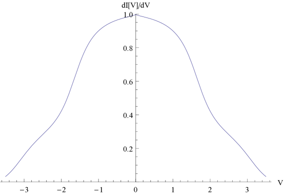
Figure 1: $\frac{dI}{dV}$ the differential conductivity for the Andreev crossed reflection

We find that for a pair of vortices the Andreev crossed reflection obeys $\frac{dI(V)}{dV}|_{V\rightarrow 0}\longrightarrow\frac{e^{2}}{h}$ (see fig.$1$) and for a single vortex $\frac{dI(V)}{dV}\rightarrow 0$.

XII-Detection of the Majorana Fermions for two metallic rings pierced by a magnetic flux which by $p-wave$

We consider a situation where two metallic rings are attached to the two ends of the $p-wave$ (which has two zero modes at the of the wire, $\gamma_{1}$ and $\gamma_{2}$) (see rings ; davidMajorana ).

We consider the special case where $L=Nl$ ($L$ is the wire length and $l$ length of each ring ) The flux in ring one is $f_{1}$ and in ring two is $f_{2}$. Using periodic boundary conditions $C_{1}(-l)=C_{1}(0)$ and $C_{2}(-l)=C_{2}(0)$ we perform a gauge transformation $\hat{C}_{1}(x)=e^{i\frac{2\pi x}{l}f_{1}}C_{1}(x)$, $\hat{C}_{2}(x)=e^{i\frac{2\pi x}{l}f_{2}}C_{2}(x)$ which introduce twisted boundary conditions. We find the spectrum of the uncoupled rings as a function of the momentum $\frac{2\pi}{l}n$, $n=0,\pm 1,\pm 2,...$.

$$H_{0}=\sum_{n}\frac{\hat{\gamma}}{2}\hat{C}_{1}^{\dagger}(n)(n+f_{1})^{2}\hat{C}_{1}(n)+\sum_{n}\frac{\hat{\gamma}}{2}\hat{C}_{2}^{\dagger}(n)(n+f_{2})^{2}\hat{C}_{2}(n)$$ (70)

$H^{Maorana}=\epsilon_{0}\zeta^{\dagger}\zeta$ is the Hamiltonian of the $p-wave$ wire restricted only to the Majorana modes. We express the Majorana fermions in terms of the fermion fields $\zeta$ and $\zeta^{\dagger}$,

$$\gamma_{1}=\frac{1}{\sqrt{2}}\Big{[}\zeta^{\dagger}+\zeta\Big{]},\hskip 7.22743pt\gamma_{2}=\frac{1}{i\sqrt{2}}\Big{[}\zeta^{\dagger}-\zeta\Big{]}$$ (71)

The coupling between the wire and the two rings takes the form :

$$H_{t}=\frac{g}{\sqrt{2}}\sum_{n}\Big{[}(\hat{C}_{1}^{\dagger}(n)(\zeta+\zeta^{\dagger})+(\zeta+\zeta^{\dagger})\hat{C}_{1}(n))\Big{]}+(-i)\frac{g}{\sqrt{2}}\sum_{n}\Big{[}(\hat{C}_{2}^{\dagger}(n)(\zeta-\zeta^{\dagger})+(\zeta-\zeta^{\dagger})\hat{C}_{2}(n))\Big{]}$$

We integrate the rings degree of freedom and obtain an effective Majorana impurity Hamiltonian.

$$H_{eff}=\hat{\zeta}^{*T}(\omega)\Big{[}M(\omega;f_{1},f_{2})\Big{]}\hat{\zeta}(\omega);\hat{\zeta}^{*T}(\omega)=\Big{[}\zeta^{\dagger}(\omega),\zeta,(\omega),\zeta^{\dagger}(-\omega),\zeta(-\omega)\Big{]}$$ (73)

$M(\omega)$ is a $4\times 4$ matrix which depends on $\Delta$ and $\delta$ (the function obtained by integrating the ring degrees of freedom) . $\Delta$ and $\delta$ are given by:

$\Delta=\frac{g^{2}}{8}(\Delta^{(1)}+\Delta^{(2)})$, $\delta=\frac{g^{2}}{8}(\Delta^{(1)}+\Delta^{(2)})$, $\Delta^{(1)}=\sum_{n}\Big{[}\frac{\omega-E_{1}(n)+ix}{(\omega-E_{1}(n))^{2}+x^{2}}\Big{]}$ , $\Delta^{(2)}=\sum_{n}\Big{[}\frac{\omega-E_{2}(n)+ix}{(\omega-E_{2}(n))^{2}+x^{2}}\Big{]}$ ,$x\rightarrow 0$.

The matrix $M(\omega)$ is given by:

$M_{1,1}(\omega)=\omega-\epsilon_{0}-\Delta$, $M_{1,2}(\omega)=M_{1,3}(\omega)=0$,$M_{1,4}(\omega)=-\delta$; $M_{2,1}(\omega)=0$, $M_{2,2}(\omega)=-(\omega+\epsilon_{0})+\Delta$, $M_{2,3}(\omega)=\delta$, $M_{2,4}(\omega)=0$; $M_{3,1}(\omega)=0$ ,$M_{3,2}(\omega)=\delta$, $M_{3,3}(\omega)=-(\omega+\epsilon_{0})+\Delta$, $M_{3,4}(\omega)=0$; $M_{4,1}(\omega)=\delta$,$M_{4,2}(\omega)=M_{4,3}(\omega)=0$, $M_{4,4}(\omega)=(\omega+\epsilon_{0})-\Delta$; $E_{1}(n)=\frac{\kappa}{2}(n+f_{1})^{2}-\mu$; $E_{2}(n)=\frac{\kappa}{2}(n+f_{2})^{2}-\mu$.

We integrate the Majorana Fermion and obtain the exact partition function:

$$\mathbf{Z}(f_{1},f_{2})=Z(g=0;f_{1},f_{2})\cdot det[M(\omega;f_{1},f_{2})]$$ (74)

$Z(g=0)$ is the partition function for two uncoupled rings. The effect of the coupling is controlled by the Majorana contribution $det[M(\omega;f_{1},f_{2})]$. Therefore the current is given by $I_{1}(f_{1},f_{2})=\Big{[}\frac{dLog(\mathbf{Z}(f_{1},f_{2}))}{df_{1}}\Big{]}$ ; $I_{2}(f_{1},f_{2})=\Big{[}\frac{dLog(\mathbf{Z}(f_{1},f_{2}))}{df_{2}}\Big{]}$. Due to the multiplicative form of the partition function the current is a sum of two parts $I_{i}(f_{i};g=0)$ (i=1,2) and a second part is determined by the matrix $M(\omega;f_{1},f_{2})$ and is given by $\delta I_{i}(f_{1},f_{2})$ , $i=1,2$ . The current in each ring is given by,

$$I_{1}(f_{1},f_{2})=I_{1}(f_{1};g=0)+\delta I_{1}(f_{1},f_{2};M)$$

$$I_{2}(f_{1},f_{2})=I_{2}(f_{2};g=0)+\delta I_{2}(f_{1},f_{2};M)$$

We investigate the case of equal fluxes, $f_{1}=f_{2}=f$. Due to the fact that $L=Nl$ the hoping matrix elements are real. In particular the Majorana energy $\epsilon_{0}$ couple like a regular impurity to a set of states determined by the two rings . Effectively the integration of the electrons in the rings renormalizes the energy $\epsilon_{0}$ to $\epsilon_{eff.}(\epsilon_{0},f)=\epsilon_{0}+\Sigma(f)$ where $\Sigma(f)$ is the shift in energy caused by the energy in the ring $E(n,f)$.

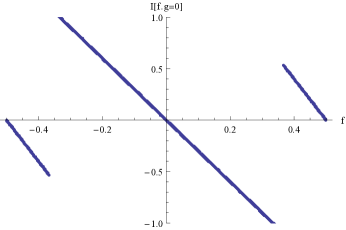
Figure 2: The current for a single ring, the coupling constant to the wire is zero. The current was computed for a fixed chemical potential,this explains the jump of the current at $f=\pm 0.4$.

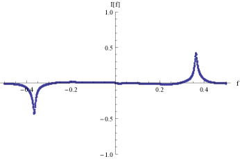
Figure 3: The shift of the persistent current for the Majorana energy(two rings) $\epsilon_{0}=0.01$ .

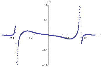
Figure 4: The shift of the persistent current for the Majorana energy (two rings) $\epsilon_{0}=0.1$ .

This result show that when the Majorana energy goes to zero the only contribution to the persistent current comes from the perfect wire in figure $2$ .In the presence of a Majorana Fermion we have in addition to the persistent current from the perfect wire the contributions $\epsilon_{eff.}(\epsilon_{0},f)=\epsilon_{0}+\Sigma(f)$ determined by the matrix $M(\omega)$ given in fig.$3$ for the Majorana energy $\epsilon_{0}=0.01$ and in fig.$4$ for the Majorana energy $\epsilon_{0}=0.1$. The persistent current is measured by scanning with the SQUID Moler which measures the change in the magnetization (The magnetization is proportional to the persistent current). One subtract from the value of the persistent current, the current from a single ring , and find the dependence of the persistent current (the correlation part given by $\delta I_{i}(f_{1},f_{2})$ , $i=1,2$) on the Majorana energy. From the result obtained here it is suggested that for two different fluxes,$f_{1}\neq f_{2}$ the effect of the fluxes will be local . The correlation between the currents the two rings is negligible.

In the past only measurements of few rings was possible . In recent years some of the experimental groups have claimed to measure the persistent current in a single ring. Some of the complications are related to the fact that the measurements have been done in diffusive limit (with 10-20 rings) and not in the ballistic limit which is considered in our calculation. The effect of the diffusive limit can be study by coupling the rings to a noise bath.

XIII- Conclusions

In conclusion the method of curved spaces introduced in the context of the Spin Hall effect has been applied to Topological Insulator and Weyl Semimetals. The method consists on the fact that in momentum space the coordinates are given by a momentum derivative, due to the fact that the spinor changes in the B.Z. the coordinate becomes covariant. The appearance of the spin connections in the covariant derivative generates the curvature. The Topological invariants, the Chern number are obtained after we impose the constraints time reversal, or charge conjugation ( for Superconductors). The Chern number are given by the covariant coordinates commutators. The formalism allows to obtain new Heisenberg equation of motion which depends on the momentum curvature and real space curvature (magnetic fields). In particular the formalism is well suited to discuss $T.I.$ or Weyl Semimetals on curved surfaces. The Weyl Semimetals are characterized by monopoles and antimonopoles which can be investigated using a new set of complete eigenfunctions coined harmonic monopoles.

For the Topological Superconductors we considered the effect of the Majorana fermions on coupled metallic rings and computed the differential conductivity for the Andreev crossed reflection.

Appendix A

The physics of electrons in a periodic crystal is determined by the eigenvectors (spinors) $|U_{n}(\vec{k})\rangle$ ($n$ is the band-spin index) behavior in the Brillouin Zone $\vec{k}\in T^{d}$ (torus in a $d$ dimensional momentum space). This behavior is similar to the parallel transport of a vector around a curve. We need to find the way the eigenvectors change under transport in the Brillouin Zone davidSpinorbit ; Blount ; Zak1 ; Zak2 ; Zak . The topological properties are encoded into the connection $\mathcal{A}_{i}$ (the vector potential in the momentum space) which measures the changes of $|U_{n}(\vec{k})\rangle$ when it is transported in the Brillouin Zone. The changes are given by:

$id|U_{n}(\vec{k})\rangle-\Gamma^{m}_{i;n}dk^{i}|U_{m}(\vec{k})\rangle=0$ (an index which appears twice implies a summation ). The matrix $\Gamma^{m}_{i;n}$ is given by $\Gamma^{m}_{i;n}\equiv i\langle U_{n}(\vec{k})|\partial_{k^{i}}|U_{m}(\vec{k})\rangle=\mathcal{A}^{(n,m)}_{i}(\vec{k})$ where $\mathcal{A}$ is the connection. Applying twice the (exterior) derivative we define the curvature $\mathcal{F}=d(d|U_{n}(\vec{k})\rangle$ ( see Eqs.$7.145-7.145$ , Nakahara (2008) page 285 Nakahara ) and find :

$\mathcal{F}=d(d|U_{n}(\vec{k})\rangle)=\Big{[}[\partial_{j}\Gamma^{l}_{i;n}(\vec{k})+\Gamma^{m}_{j;n}(\vec{k})\Gamma^{l}_{i;m}(\vec{k})]dk^{i}\wedge dk^{j}\Big{]}|U_{l}(\vec{k})\rangle=\frac{1}{2}[F_{i,j}]_{n,l}dk^{i}\wedge dk^{j}|U_{l}(\vec{k})\rangle$ ; ( the symbol $\wedge$ represents the wedge product )

$[F_{i,j}]_{n,m}=\partial_{i}\mathcal{A}^{(n,m)}_{j}(\vec{k})-\partial_{j}\mathcal{A}^{(n,m)}_{i}(\vec{k})+i[\mathcal{A}^{(n,l)}_{i}(\vec{k}),\mathcal{A}^{(l,m)}_{j}(\vec{k})]$,

where $F_{i,j}$ is the matrix curvature with the matrix elements $[F_{i,j}]_{n,m}$ given in terms of the commutator of the covariant derivative $\hat{R}_{i}=\hat{r}_{i}+\mathcal{A}^{(n,m)}_{i}$ , $\hat{r}_{i}=i\partial_{k^{i}}$ ; $[\hat{R}_{i},\hat{R}_{j}]=F_{i,j}$.

Appendix B

Topological invariant in two space dimensions using the topological invariant in four space dimensions.

The topological response for time reversal invariant systems in one and two space dimensions is not entirely clear . In three space dimensions we can use the Chern-Simons form $K_{3}(A,F)]$ to relate the the second Chern number $C_{2}$ in four space dimensions to three dimensions using the relation $ch_{2}=d[K_{3}(A,F)]$. In four dimensional momentum space the second Chern number $C_{2}$ is given by an index operator. In analogy with the index operator for the Dirac equation I introduce the index operator in the momentum space $Ind.\Big{[}i\mathbb{R}_{4}\Big{]}$:

$$Ind.\Big{[}i\mathbb{R}_{4}\Big{]}=Tr\Big{[}\gamma^{5}e^{-\epsilon\int\,d^{4}k\bar{C}(\vec{k})\Big{(}i\mathbb{R}_{4}(\vec{k})\Big{)}^{2}C(\vec{k})}\Big{]}|_{\epsilon\rightarrow 0}\longrightarrow C_{2}$$ (76)

The operator $i\mathbb{R}$ is defined in terms of the non-Abelian spin connection :

$$A^{\alpha,\beta}_{a}(\vec{k})\equiv\langle U_{\alpha}(\vec{k})|i\partial_{a}|U_{\beta}(\vec{k})\rangle$$

$$i\mathbb{R}_{4}(\vec{k})=i\sum_{a=1,2,3,4}(\gamma_{a}(x^{a}+A_{a}(\vec{k}))\equiv i\gamma_{a}X^{a}(\vec{k})$$

$$\gamma^{5}=\left[\begin{array}[]{rrr}-1&0\\ 0&1\\ \end{array}\right]$$ (79)

$\gamma^{5}$ separates the conduction band from the valence band.

In order to show that the index operator in four space dimensions is related to the index operator in d=2 space dimensions, we introduce the transformation :

$$\mathcal{A}^{g(\theta)}(\vec{k})=g^{-1}(\theta,\vec{k})\Big{(}\mathcal{A}(\vec{k})+d\Big{)}g(\theta,\vec{k})$$ (81)

where $\theta$ parametrizes the $S^{1}$ circle (see figure $13.4$ page $521$ Nakahara ). Next we construct a family of gauge fields:

$$\mathcal{A}^{t,\theta}\equiv t\mathcal{A}^{g(\theta)};\hskip 7.22743pt0\leq t\leq 1$$ (82)

The parameters $(t,\theta)$ form a disc $D^{2}$ with $\partial D^{2}=S^{1}$ . We construct from$D^{2}\times S^{2}$ a manifold $S^{2}\times S^{2}$ . We will call the patch $(t,\theta)$ the northern hemisphere $U_{N}$ and $(s,\theta)$ the south hemisphere $U_{s}$ and the equator $S^{1}$ of $S^{2}$ corresponds to $t=s=1$ (see the figure with the two half sphere, figure $13.4$ page $521$ in Nakahara ). The gauge potential in $2+2$ dimensions can be written as:

$$\mathbb{A}_{N}(t,\theta,\vec{k})=\Big{[}0,0,\mathcal{A}^{t,\theta}(\vec{k})+g^{-1}(\theta,\vec{k})d_{\theta}g(\theta,\vec{k})\Big{]}$$

$$\mathbb{A}_{N}(t,\theta,\vec{k})=\Big{[}0,0,\mathcal{A}(\vec{k})\Big{]}$$

$\mathcal{A}(\vec{k})$ is the non-Abelian spin connection in two space dimensions. On the equator $t=s=1$ we have :

$$\mathbb{A}_{N}=g^{-1}\Big{(}\mathbb{A}_{s}+d+d_{\theta}+d_{t})g$$ (84)

where $d$ is the exterior derivative Nakahara in two dimensions, $d_{\theta}$ is the external derivative on $S^{1}$ and $d_{t}g=0$. $\mathbb{A}=(\mathbb{A}_{N},\mathbb{A}_{S})$ is the spin connection in $2+2$ dimensions. We use the relation,

$$det\Big{[}i\hat{D}(\mathcal{A}^{g(\theta)})(\vec{k})\Big{]}\equiv\Big{[}\det(i\mathbb{R}(\mathcal{A}(\vec{k}))\Big{]}^{\frac{1}{2}}e^{iw(\mathcal{A},\theta)}$$ (85)

$|det[i\hat{D}]|$ is gauge invariant and only $det[i\hat{D}]$ might have anomalous behavior . On the boundary disc $\partial D^{2}=S^{1}$ the phase $e^{iw(\mathcal{A},\theta)}$ defines the maping $\partial D^{2}\rightarrow S^{1}$

$$i\hat{D}(A)=i\sum_{a=1,2,3,4}(\gamma_{a}(x^{a}+iA_{a}(\vec{k})P_{+}),\hskip 7.22743ptP_{+}=\frac{1}{2}(1+\gamma^{5})$$ (86)

$|det[i\hat{D}(A)]|$ is gauge invariant and only the phase $w(\mathcal{A},\theta)$ is anomalous and gives the winding number $\nu_{1}$, on the disc $D^{2}$ there are points at which $det[i\hat{D}(A)]$ vanishes. The index $Ind.\Big{[}i\mathbb{R}_{2+2}\Big{]}$ is given by,

$$Ind.\Big{[}i\mathbb{R}_{2+2}\Big{]}=\int_{S^{2}\times S^{2}}c_{2}(\mathbb{F})=\nu_{1}$$ (87)

where the curvature $\mathbb{F}$ is given by,

$$\mathbb{F}=(d+d_{\theta}+d_{t})\mathbb{A}+\mathbb{A}^{2}$$ (88)

$\nu_{1}$ is the winding number which is is even or odd and corresponds to the index $Z_{2}$ introduced earlier.

Following the procedure used before which relates the Chern character to the Chern-Simons form $c_{2}=d[K_{3}(A,F)]$ we find:

$$\int_{S^{2}\times S^{2}}c_{2}(\mathbb{F})=\int_{D^{2}\times S^{2}}c_{2}(\mathbb{F}_{N})+\int_{D^{2}\times S^{2}}c_{2}(\mathbb{F}_{S})=\int_{S^{1}\times S^{2}}\Big{[}K_{2+1}(\mathbb{A}_{N},\mathbb{F}_{N})|_{t=1}-K_{2+1}(\mathbb{A}_{S},\mathbb{F}_{S})|_{s=1}\Big{]}$$ (89)

Since $\int_{S^{1}\times S^{2}}K_{2+1}(\mathbb{A}_{S},\mathbb{F}_{S})=0$ we find:

$$Ind.\Big{[}i\mathbb{R}_{2+2}\Big{]}=\int_{S^{1}\times S^{2}}K_{2+1}(\mathbb{A}_{N},\mathbb{F}_{N})=\int_{S^{1}\times S^{2}}K_{2+1}(\mathcal{A}^{g(\theta)}+g^{-1}d_{\theta}g,\mathcal{F}^{g(\theta)})=-(\frac{1}{2\pi})^{2}Tr[Wd\mathcal{A}]$$ (90)

where $W\equiv g^{-1}(\theta)d_{\theta}g(\theta)$. For $\theta=0$ we find $W=1$ and $Ind\Big{[}i\mathbb{R}_{2+2}\Big{]}=\nu_{1}$ ($\nu_{1}$ is the winding number ) which is identical to the $Z_{2}$ index introduced by Kane .

The procedure presented here allows a direct construction of the $Z_{2}$ invariant in two dimensions as an emergent object from four dimensions and therefore is related to the electromagnetic or sound wave response defined in four space dimensions. Contrary to early procedures which used dimensional reduction the procedure proposed is based on deforming the spin connection $\mathcal{A}$ to a family of higher dimensions gauge potentials $\mathcal{A}^{g(\theta)}$.

References

• (1) B.A.Volkov and O.A. Pankratov ”Two dimensional massless electrons in an inverted contact” JETP LETT. vol.42,179(1985)
• (2) M.Z.Hasan and J.E. Moore ”Three -dimensional topological Insulators” Anual Review of Condensed matter Physics ,2:55,(2011)
• (3) F.D.M. Haldane ”Model For Quantum Hall Without Landau Levels ” Phys.Rev.Lett.61,2015(1988)
• (4) Pavan Hosur, S.A. Prameswaran and Ashvin Vishwanath ”‘Charge transport in Weyl semimetals ”‘ Phys.Rev.Lett. 108,046602(2012)
• (5) Yi Li and F.D.M.Haldane ”Topological Nodal Cooper pairing in doped Weyl metals” arXiv:1510.0173
• (6) R.Okugawa and S.Murakami arXiv:1402.7145v2
• (7) A.A.Soluyanov, D.Grech, Z.Wang,Q.Wu,M.Troyer,Z.Dai, and B.A.Bernevig arXiv:1507.01603
• (8) M.F.L.Golterman, K.Jansen and D.B. Kaplan ”Chern-Simons Currents and Chiral Fermions on the Lattice ” Phys.Lett.B301, (1993)219-223.
• (9) Michael Creutz and Ivan Horwath ”Surface States and Chiral Symmetry On The Lattice” Phys.Rev.D50,2297(1994)
• (10) C.L. Kane and E.J. Mele ”Quantum Spin Hall Effect In Graphene ” Phys.Rev. Lett. 95 226801 (2005)
• (11) C.L. Kane and E.J. Mele ”$Z_{2}$ Topological Order And The Quantum Spin Hall Effect ”Phys.Rev.Lett. 95,146802(2005).
• (12) D.Schmeltzer,”Topological Spin Current Induced By Non-Commuting Coordinates: An application to the Spin-Hall Effect ”Phys.Rev.B 73,165301(2006) and ”Topological Spin Current” arXiv:cond-mat/0406565(2004)
• (13) M.Nakahara, ”Geometry,Topology and Physics” Taylor and Francis Group ,New York ,London (2003)
• (14) H.T. Nieh ”Gauss-Bonnet and Bianchi identities in Riemann-Cartan type gravitational theories” J.Math.Phys.21(6), June 1980
• (15) J.E.Moore and L.Balents ”Topological Invariants of Time-Reversal-Invariant Band Structures” Phys.Rev.B 75,121306(2007)
• (16) J. W. McIver, D. Hsieh, H. Steinberg ,PJarillo-Herrero and N.Gedik ,Nat.Nanotech ”Control over topological Insulator photocurrents with light polarization” 7,96 (2011).
• (17) A.Junck,Gil Reael, and Felix Oppen ” Photocurrent Response of Topological Insulators Surface states ” arXiv:1301.4392 (2013)
• (18) Edwart Witten ”Non-Abelian Bosonization in Two Dimensions” Comun.Math.Phys.92 ,455-472 (1984)
• (19) Andrew M. Essin Joel E.Moore and David Vanderbilt ”Magnetoelectric Polarizability and Axion Electrodynamics In Cristalline Insulators” Phys.Rev.Lett.102,146805(2009)
• (20) M.M.Vazifeh and M.Franz ”Quantization and 2$\pi$ periodicity of axion action in topological insulators”’Phys.Rev.B82,233103(2010)
• (21) D.A.Ivanov ”Non-Abelian of Half-Quantum Vortices in a p-Wave Superconductors” Phys.Rev.Lett.86,268(2001)
• (22) D.Schmeltzer and A.Saxena, ”Chiral P-wave Superconducting nanowire coupled to two metallic rings pierced by a flux ” Phys.Rev.B.86, 094519(2012).
• (23) Xiao-Liang Qi, Taylor Hughes and Shou-Cheng Zhang ”Topological Field Theory Of Time Reversal Invariant Insulators” Phys.Rev.B78,195424(2008)
• (24) Xiao-Liang Qi and Shou-Cheng Zhang ”Topological Insulators and Superconductors” Rev.of Modern Physics 831057 (2011).
• (25) Andreas P.Schnyder , Shinsei Ryu, Akira Furusaki, Andreas W.W. Ludwig ”Classification Of Topological Insulators and Superconductors In Three Spatial dimensions” Phys.Rev.B78,195125(2008)
• (26) J.G.Checkelsky,R.Yoshimi,A. Tsukazaki, K.S.Takahashi ”Trajectory of Anomalous Hall Effect toward the Quantized State in a Ferromagnetic Topological Insulator” arXiv:1406.7450v1
• (27) Chao-Xing Liu et al, ”Model Hamiltonian for Topological Insulators ” Physical Review B 82, 045122 (2010)
• (28) Johan Nilson,A.R. Akhmerov,and C.W.J. Beenakker”Spiting of a Cooper Pair by a Pair of Majorana Bound States” Phys.Rev.Lett.101,120403(2008)
• (29) K.T.Law,Patrick A.Lee,and T.K. Ng”Majorana Fermion induced Resonant Andreev Reflection” Phys.Rev.Lett.103,237001(2009)
• (30) Lucasz Fidkowski, Jason Alicea, Netanel H.Lindner,Roman M. Lutchyn ,and Mathew P.A. Fisher ”Universal transport signature of Majorana fermions in superconducting -Luttinger liquid junctions” Phys.Rev.B85,245121(2012)
• (31) Jian Li,Genevieve Fleury,and Markus Buttiker ”Scattering theory of chiral Majorana fermion intereferometry” Phys.Rev.B85,145440(2012)
• (32) Karsten Flensberg ”Tunneling characteristics of a chain of Majorana bound states” Phys.Rev.B82,180516(R)(2010)
• (33) Benjamin J. Wieder ,Fan Zhang,and C.L. Kane ”Signature of Majorana fermions in topological insulator Josephson junction devices ” Phys.Rev.B89,075106(2012) arXiv:1309.0163v1
• (34) Liang Fu and C.L. Kane ”Probing Neutral Majorana Fermion Edge Modes with Charge Transport” Phys.Rev.Lett.102,216403(2009)
• (35) V.Orlyancik, M.P. Stehno, P.Ghaemi,M. Bralek, N.Koirala,S.Oh, and D.J. Van Harlingen ” Signature of Topological phase transition in the Josephson supercurrent through a topological insulator”
• (36) D.Schmeltzer , ”Quantum Mechanics For Genus g=2 Persistent Current in Coupled Rings”J. Phys:Condens Matter 20 335205(2008).
• (37) P.Rammond ”Field Theory A Modern Primer” The Benjamin /Cummings Publishing company , (1981) pages 317-330.
• (38) Steven Weinberg ”Theory Quantum Theory of Fields - volume II” (pages 445-450 ,eq.23.4.1) ,Cambridge University Press (1996)
• (39) D.Schmeltzer ,and Hsuan-Yeh Chang ,”Rectified voltage induced by a microwave field in a confined two-dimensional electron gas with a mesoscopic static vortex” PMC Physics B 2008, 1:14 ,October 21 (2008).
• (40) D.Schmeltzer and A.Saxena ”Magnetoelectric effect induced by electron-electron interaction in three dimensional topological Insulators ” Physics Letters A 377 (2013) 1631-1636
• (41) D.Schmeltzer and A.Saxena ”The wave functions in the presence of constraints-persistent Current in Coupled Rings ” Phys.Rev.B 81 ,195310 (2010).
• (42) Hendryik Bluhm, Nicholas C. Koshnick, Julie A.Bert, Martin E.Hubert and Kathryin A.Moler ” Persistent currents in normal metal rings” Phys.Rev.Lett.102,136802 (2009)
• (43) D.Schmeltzer ”A-Geometrical approach to topological insulators with edge dislocations ” New Journal of Physics 14,063025 (2012)
• (44) J.Rammer ”Quantum Field Theory of Non-Equilibrium States” (Cambridge University Press , Cambridge ,UK,2007), pp.377-389.
• (45) D. Schmeltzer, ”Topological Insulators-transport in curved space” , arXiv:1012.5871 and Advances in Condensed Matter and Materials Research ,volume 10 Editors:Hans Geelvinck and Sjaak Reyst ,chapter 9, pages 379-403(2011).
• (46) D.Schmeltzer ”Propagation of Phonon in Topological Superconductors induced by strain fields instantons” International Journal of Modern Physics B vol.28,1450059 (2014)
• (47) D.Schmeltzer and Avadh Saxena ” Interference effects for $T^{2}=-1$ time reversal invariant topological insulators : Surface Optical and Raman conductivity” Phys.Rev.B 88,035140 (2013)
• (48) D.Schmeltzer and K. Ziegler ” Optical conductivity for the surface of a Topological Insulator ” arXiv:1302.4145
• (49) Zohar Ringel ,Yaacov E.Kraus, and Ady Stern ”Strong side of weak topological insulators” Phys.Rev.B86,045102(2012)
• (50) E.I. Blount ”‘Formalism of Band Theory”’ Solid State Physics edited by F.Seitz and D. Turnubul , (Academic, New York ,1962),Vol.13, pages 305-375.
• (51) M.V.Berry ”Quantal Phase Factors Accompanying Adiabatic Changes” ,Proc.R.Soc.A392,45(1984).
• (52) D.Thouless,M.Kohmoto,M.Nightingale et M.den.Nijs, ”Quantized Hall Conductance In a Two-Dimensional Periodic Potential” Phys.Rev.Lett.49, 405 (1982).
• (53) B.Simon ”Holonomy the Quantum Adiabatic Theorem and Berry Phase ” Phys.Rev.Lett.51,2167 (1983).
• (54) V.Gourarie ”Single - particle Green’s functions and interacting topological insulators” Phys.Rev.83,085426 (2011)
• (55) Zhong Wang and Shou-Cheng Zhang ”Simplified Topological Invariants for Interacting Insulators” arXiv:1203.1028v3
• (56) K.Fujikawa ”Path integral for gauge theories with fermions” Phys.Rev.D. 21,2848(1980)
• (57) Anndrew P.Schneider and Shinsei Ryu ”Topological phases and surface flat bands in superconductors whithout inversion symmetry” Phys.Rev.B. 84,060504(R)(2011)
• (58) Liang Fu ”Topological Crystalline Insulators” Phys.Rev.Lett.106,106802(2011)
• (59) Timothy H.Hsieh, Hsin Liu, Wenhui Duan, Arun Bansil and Liang Fu ” Topological crystalline insulators in the SnTe material classes ” arXiv: 1202.1003 v2
• (60) Michael Stone and Paul Goldbart ”Mathematics for Physics -A guided tour for graduate students ”, page 433 eq.12.63 , Cambridge University Press (2009)
• (61) Wu.C.B., A. Bernewig and Shou-Cheng Zhang ”‘The Helical Liquid and The Edge Of Quantum Spin Hall Systems”’ Phys.Rev.Lett. 96, 106401 (2006).
• (62) Chao-Xing Liu, X.L. Qi, H.Zhang,Xi Dai,Z. Fang and Shou-Cheng-Zhang ”Model Hamiltonian for topological insulators” Phys.Rev.B 82,045122(2010)
• (63) Chao-Xing Liu ,H.Zhang ,B.Yan, X.L. Qi, T.Frauenheim ,Xi Dai, Z. Fang and Shou-Cheng-Zhang ”Oscillatory crossover from two dimensional to three-dimensional topological insulators” Phys.Rev.B 81041307R (2010)
• (64) Shinobu Hikami ,”Anderson localization in a nonlinear -sigma model representation ” Phys.Rev.B 24,2671(1981)
• (65) A.A.Taskin,S.sasaki ,K.Segawa and Y. Ando ,”Quantum Oscillations in a Topological Insulator” Phys.Rev.Lett. 109,066803 (2012)
• (66) Hai-Zhou Lu, Junren Shi, and Shun-Qing Shen, ” Competition between localization and antilocalization in topological surface states ” Phys.Rev.Lett.107,076801(2011)
• (67) S.Doniach and E.H.Sondheimer ”Green’s Functions for Solid-State Physicists” (Imperial College Press,Oxford , London,UK,1988)
• (68) H.Peng et.al ”Aharonov-Bohhm interference in Topological Insulator Nanoribbons ” Nature Materials,9, 225 -229 (2010)
• (69) Yi Zhang and Ashvin Viswanath ”Anomalous Aharonov -Bohm
• (70) T.Hanaguri et al. ”Momentum-Resolved Ladau Level Spectroscopy of Dirac Surface States ”Phys.Rev.Lett.82,081305(2010)
• (71) R.Biswas and A.V. Balatsky ”Impurity-Induced On The Surface Of the Three -Dimensional Topological Insulator ” Phys.Rev.B 81,23405 (2010)
• (72) J.Chen, X.Y. He, K.H. Wu, Z.Q.Ji,L.Lu,J.R. Shi,J.H.Smet and Y.Q.Li”Tunable surface conductivity in $Bi_{2}Se_{3}$ revealed in diffusion electron transport” Phys.Rev.B. 83,241304(R)(2011)
• (73) Ayelet Pnueli ”Spinors and Scalars on Riemann Surfaces ”J.Phys. A: Math.Gen.27,
• (74) Dung-Hai Lee ”Surface States of Topological Insulators : The Dirac Fermions in Curved Two-Dimensional Spaces” Phys.Rev.Lett103,196804(209).
• (75) I.Alicea,” New directions in the pursuit of Majorana fermions in solid state systems”, Rep. Prog. Phys. 75,076501 (2012).
• (76) B.Andrei Bernevig and Taylor L.Hughes ”Topological Insulators and Superconductors ” 2013 Princeton University Press,Princeton and Oxford.
• (77) D. P. Arovas and J. A. Freire, ”Dynamical vortices in superfluid films” Phys. Rev. B55, 1068(1997)
• (78) Tai Tsun Wu and Chen Ning Yang, Nuclear Physics B107 (1976) 365-380
• (79) Eric J.Weinberg arXiv:hep-th/930805(1993)
• (80) Daniel Boyanovsky ” Field Theory of The Two Dimensional Ising Model: Conformal Invariance ,Order, Disorder , and Bosonization”’ Phys.Rev.B.39, 6744(1989).
• (81) D.Schmeltzer et al. ”Spin-Polarized Conductance Induced by Tunneling Through a Magnetic Impurity ”‘ Phys.Rev.Lett90,116802(2003)
• (82) Jukka I. Vayrynen, Moshe Goldstein, and Leonid I. Glazman ”Helical edge resistance introduced by charged puddles” arXiv:1303.1766v1.
• (83) D.Schmeltzer ”Dirac’s Method For Constraints : An application To Quantum Wires” J.Phys:Condens.Matter 23 155601 (2011).
• (84) D.Schmeltzer ,”The Marginal Fermi Liquids - An Exact Derivation Based on Dirac’s First Class Constraints Method”, Nuclear Physics B 829,447-477 (2010)
• (85) D.Schmeltzer ”A microscopic model for detecting the surface states in Topological Insulators” arXiv:1310.6798(2013)
• (86) J. Zak, ”Dynamics Of Electrons In Solids In External Fields”, Phys. Rev. 168,687 (1968).
• (87) J. Zak, ”Dynamics Of Electrons In Solids In External Fields,II”’, 177,1151 (1969).
• (88) J. Zak, ”Berry Phase for energy Bands In Solids”, Phys. Rev. Lett. 62, 2747 (1989) .
• (89) H.M. Guo. S.Q. Shen, ”Topological phases in one-dimensional interacting fermion system” Phys.Rev.B84, 195107(2011)
• (90) Shinsey Riu, Joel Moore and Andreas W.W. Ludwig, ” Electromagnetic and gravitational responses and anomalies in topological insulators and superconductors ” Phys.Rev.B 85,045104 (2012)
• (91) Zhong Wang Xiao-Liang Qi and Shou-Cheng Zhang, ”Topological field theory and thermal responses of interacting topological superconductors ” Phys.Rev. B 84,014527(2011)
• (92) Alex Kamenev ”‘Field Theory of No-Equilibrium Systems ”Cambridge University Press (2011)
• (93) L.D.Landau and E.M.Lifshitz ”Theory of Elasticity” Elsevier third edition ( 1986)
• (94) Claudio Chamon, Andreas W.W. Ludwig and Chetan Nayak ” Keldish approach to disorder and interacting electron systems :Derivation of Finkelstein’s renormalozation-group equations” Phys.Rev.B 60,2239(1999).