Stability Analysis of Slotted Aloha with Opportunistic RF Energy Harvesting

Abstract

Energy harvesting (EH) is a promising technology for realizing energy efficient wireless networks. In this paper, we utilize the ambient RF energy, particularly interference from neighboring transmissions, to replenish the batteries of the EH enabled nodes. However, RF energy harvesting imposes new challenges into the analysis of wireless networks. Our objective in this work is to investigate the performance of a slotted Aloha random access wireless network consisting of two types of nodes, namely Type I which has unlimited energy supply and Type II which is solely powered by an RF energy harvesting circuit. The transmissions of a Type I node are recycled by a Type II node to replenish its battery. We characterize an inner bound on the stable throughput region under half-duplex and full-duplex energy harvesting paradigms as well as for the finite capacity battery case. We present numerical results that validate our analytical results, and demonstrate their utility for the analysis of the exact system.

Index Terms—Wireless networks, slotted Aloha, opportunistic energy harvesting, interacting queues.

I Introduction

One of the prominent challenges in the field of communication networks today is the design of energy efficient systems. In traditional networks, wireless nodes are powered by limited capacity batteries which should be regularly charged or replaced. Energy harvesting has been recognized as a promising solution to replenish batteries without using any physical connections for charging. Nodes may harvest energy through solar cells, piezoelectric devices, RF signals, etc. In this paper, we focus on RF energy harvesting. Recent studies present experimental measurements for the amount of RF energy that can be harvested from various RF energy sources. Two main factors affect the amount of RF energy that can be harvested, namely, the frequency of the RF signal and the distance between the “interferer” and the harvesting node, e.g., see Table I in [1].
Recently, an information-theoretic study of the capacity of an additive white Gaussian noise (AWGN) channel with stochastic energy harvesting at the transmitter has shown that it is equal to the capacity of an AWGN channel under an average power constraint [2]. This, in turn, motivated the investigation of optimal transmission policies [3] for single user [4, 5, 6] and multi-user [7, 8, 9] energy harvesting networks. The optimal policy that minimizes the transmission completion time was studied in [4]. In [5], the authors studied the problem of maximizing the short-term throughput and have shown that it is closely related to the transmission completion time problem [4]. The authors in [6] studied the optimal transmission policies for energy harvesting networks under fading channels. Moreover, [7, 8, 9] extends the analysis to broadcast, multiple access, and interference channels, respectively. The authors in [10] introduced the concept of energy cooperation where a user can transfer portion of its energy, over a separate channel, to assist other users.
Significant research has also been conducted on RF energy harvesting. In [11], the author discusses the fundamental trade-offs between transmitting energy and transmitting information over a single noisy link. The author derives the capacity-energy functions for several channels. The authors in [12], extend the point-to-point results of [11] to multiple access and multi-hop channels. Recently, several techniques were proposed for designing RF energy harvesting networks (RF-EHNs), e.g., [13]. The RF energy harvesting process can be classified as follows: i) Wireless energy transfer, where the transmitted signals by the RF source are dedicated to energy transfer, ii) Simultaneous wireless information and power transfer, where the transmitted RF signal is utilized for both information decoding and RF energy harvesting, and iii) Opportunistic energy harvesting, where the ambient RF signals, considered as interference for data transmission, are utilized for RF energy harvesting. The receiver architecture may also vary as follows [13],[14]: a) Co-located receiver architecture, where the radio receiver and the harvesting circuit use the same antenna for both decoding the data and energy harvesting, and b) Separated receiver architecture, where the radio receiver and the harvesting circuit are separated, and each is equipped with its own antenna and RF front-end circuitry.
In [14], the authors discuss the practical limitations of implementing a simultaneous wireless information and power transfer (SWIPT) system. A major issue is that energy harvesting circuits are not able to simultaneously decode information and harvest energy. Hence, the authors in [14] proposed and analyzed two modes of operation for the co-located receiver architecture, that is, time switching and power splitting. Furthermore, the RF energy harvesting transceivers may also be classified as: a) Half-duplex energy harvester, where a co-located RF energy harvesting transceiver can either transmit data or harvest RF signals at a given instant of time, and b) Full-duplex energy harvester, where a node is equipped with two independent antennas and can transmit data and harvest RF signals, simultaneously. In this paper, we investigate opportunistic RF energy harvesting under the half-duplex and full-duplex modes of operation.
The cornerstone of random access medium access control (MAC) protocols is the Aloha protocol [15], which is widely studied in multiple access communication systems because of its simplicity. The applications of Aloha-based protocols range from traditional satellite networks [16] to radio frequency identification (RFID) systems [17] and the emerging Machine-to Machine (M2M) communications [18]. It is also considered as a benchmark for evaluating the performance of more sophisticated MAC protocols. Based on the Aloha protocol, nodes contend for the shared wireless medium and cause interference to each other. Hence, the service rate of a node depends on the backlog of other nodes, i̇.e., the nodes’ queues become interacting as originally characterized in [19]. Tsybakov and Mikhailov [20] were the first to analyze the stability of a slotted Aloha system with finite number of users. Rao and Ephremides [21] characterized the sufficient and necessary conditions for queue stability of the two user case, using the so-called stochastic dominance technique. In addition, they established conditions for the stability of the symmetric multi-user case. Other works followed and studied the stability of slotted Aloha with more than two users [22, 23, 24, 25]. The authors in [26] extended the stability analysis under the collision model to a symmetric multi-packet reception (MPR) model, which was later generalized to the asymmetric MPR model in [27].
Perhaps the closest to our work are [28, 29] which characterize the stability region of a slotted Aloha system with energy harvesting capabilities, under the multi-packet reception model. The authors considered a system where the nodes harvest energy from the environment at a fixed rate and, thus, the energy harvesting process is modeled as a Bernoulli process.
In this work, we analyze the stability of a slotted Aloha random access wireless network consisting of nodes with and without RF energy harvesting capability. Specifically, we consider a wireless network consisting of two nodes, namely a node of Type I which has unlimited energy supply and a node of Type II which is powered by an RF energy harvesting circuit. The RF transmissions of the Type I node are harvested by the Type II node to replenish its battery. Our contribution in this paper is multi-fold. First, we outline the difficulties in analyzing the stability of the exact RF energy harvesting Aloha system $\mathcal{S}_{O}$ and for mathematical tractability we introduce an equivalent system $\mathcal{S}_{G}$. Second, we generalize the stochastic dominance technique for analyzing RF EH-networks. Third, we characterize an inner bound on the stable throughput region of the system $\mathcal{S}_{G}$ under the half-duplex and full-duplex energy harvesting paradigms. Also, we derive the closure of the inner bound over all transmission probability vectors. Fourth, we investigate the impact of finite capacity batteries on the stable throughput region. Finally, we validate our analytical findings with simulations and conjecture that the inner bound of the system $\mathcal{S}_{G}$ is also an inner bound for the exact system $\mathcal{S}_{O}$.
The rest of this paper is organized as follows. In Section II, we present the system model and the assumptions underlying our analysis. In Section III, we describe the energy harvesting models for the systems $\mathcal{S}_{O}$ and $\mathcal{S}_{G}$. Our main results are presented in Section IV and proved in Section V. In Section VI, we investigate the impact of finite capacity batteries and full-duplex energy harvesting on the stability region of our system. We corroborate our analytical findings by simulating the systems $\mathcal{S}_{O}$ and $\mathcal{S}_{G}$ in Section VII. Finally, we draw our conclusions and point out directions for future research in Section VIII.

II System Model

We consider a wireless network consisting of two source nodes and a common destination, as shown in Fig. 1. We consider a slotted Aloha multiple access channel [15], where time is slotted and the slot duration is equal to one packet transmission time. We assume two types of nodes in our system: Type I node has a data queue, $Q_{1}$, and unlimited energy supply, while Type II node has a data queue, $Q_{2}$, and a battery queue, $B$, as shown in Fig. 1. Moreover, packets arrive to the data queues, $Q_{1}$ and $Q_{2}$, according to independent Bernoulli processes with rates $\lambda_{1}$ and $\lambda_{2}$, respectively. The transmission probabilities of Type I and II nodes are $q_{1}$ and $q_{2}$, respectively.
We assume perfect data channels, i̇.e., the destination successfully decodes a data packet, if only one node transmits. If two nodes transmit simultaneously, a collision occurs and both packets are lost and have to be retransmitted in future slots. At the end of each time slot, the destination sends an immediate acknowledgment (ACK) via an error-free feedback channel.

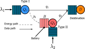
Figure 1: System model

Data packets of Type I and II nodes are stored in queues $Q_{1}$ and $Q_{2}$, respectively. The evolution of the queue lengths is given by [25]

$$Q_{i}^{t+1}=\max\{Q_{i}^{t}-Y_{i}^{t},0\}+X_{i}^{t},\ \ \ i=1,2.$$ (1)

where $X_{i}^{t}\in\{0,1\}$ is the arrival process for data packets and $Y_{i}^{t}\in\{0,1\}$ is the departure process independent of $Q_{i}$ status, i̇.e., $Y_{i}^{t}=1$ even if the data queue is empty [27]. $X_{i}^{t}$ is a Bernoulli process with rate $\lambda_{i}$ and $\mathbb{E}[Y_{i}^{t}]=\mu_{i}$.

We assume that Type II nodes operate under a half-duplex energy harvesting mode, i̇.e., they either harvest or transmit but not both simultaneously. Hence, the harvesting opportunities are in those slots when a Type II node is idle while a Type I node is transmitting. The channel between the two source nodes is a block fading channel, where the fading coefficient remains constant within a single time slot and changes independently from a slot to another. For Rayleigh fading, the instantaneous channel power gain $h_{t}$ at time slot $t$ is exponentially distributed, i̇.e., $h_{t}\sim\textit{Exp}(1)$. Let $P_{j}$ be the transmission power of node $j$, and $l$ be the distance between the two source nodes. We consider the non-singular pathloss model with $(1+l^{\alpha})^{-1}$, where $\alpha$ is the pathloss exponent. We use power and energy interchangeably throughout the paper, since we assume unit time slots. In the next section, we develop a discrete-time stochastic process to model RF energy harvesting.

III Energy Harvesting Models

Prior work largely models the energy harvesting process as an independent and identically distributed (iid) Bernoulli process with a constant rate [29]. In the following, we first study the RF energy harvesting process of the exact system $\mathcal{S}_{O}$ and show that the inter-arrival time of the energy arrivals has a general distribution. Second, we propose an equivalent system $\mathcal{S}_{G}$ where the inter-arrival time of the energy arrivals is geometrically distributed with the same mean as $\mathcal{S}_{O}$.

III-A RF Energy Harvesting Model of the exact system $\mathcal{S}_{O}$

The received power at a Type II node from the transmissions of Type I node at time slot $t$ is $P_{R}(t)=\eta P_{1}h_{t}(1+l^{\alpha})^{-1}$, where $P_{1}$ is the transmission power of Type I node and $\eta$ is the RF harvesting efficiency [13]. Recent studies demonstrated that $\eta$ typically ranges from $0.5$ to $0.7$, where its value depends on the efficiency of the harvesting antenna, impedance matching circuit and the voltage multiplier [31]. In order to develop the analytical model underlying this paper, we approximate the continuous energy arrival process in quantas of size $\gamma$ joules.

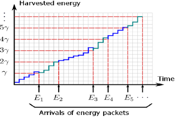
Figure 2: A unit of energy is harvested every time the accumulated energy in the battery exceeds $\gamma$.

Typically, we need to harvest RF energy from multiple transmissions of Type I node in order to accumulate $\gamma$ joules. Conceptually, accumulating $\gamma$ joules is equivalent to having a single energy packet arrival to the battery. We model the battery of a Type II node as a queue with unit energy packet arrivals from the harvesting process, and unit energy packet departures when Type II node transmits. There is an energy packet arrival to the battery queue at the end of the time slot in which the accumulated energy exceeds $\gamma$, see Fig. 2. Let $Z$ be the number of Type I transmissions needed to harvest one energy unit.

Lemma 1. For a persistent ($q_{1}\!=\!1$) and saturated Type I node, the probability mass function (PMF) of $Z$, when the channel between Type I and II nodes is modeled as a Rayleigh fading channel with parameter $h_{t}$, is given by

$$\mathbb{P}[Z=k] =\frac{e^{-\theta}\ \theta^{k-1}}{(k-1)!},\ k=1,2,\cdots,\ \text{where }\theta=\frac{\gamma(1+l^{\alpha})}{\eta P_{1}}$$ (2)

Proof.

Note that if the accumulated received energy over $k$ slots is greater than or equal to, $\gamma$ while the accumulated received energy up to slot $k-1$ is less than $\gamma$, then we need $k$ slots to harvest one energy unit.

$$\mathbb{P}[Z=k] =\mathbb{P}\left[\sum_{t=1}^{k}P_{R}(t)\geq\gamma,\ \sum_{t=1}^{k-1}P_{R}(t)<\gamma\right]$$ (3)

$$\stackrel{{\scriptstyle(a)}}{{=}}\mathbb{P}\left[\sum_{t=1}^{k-1}h_{t}<\theta\right]-\mathbb{P}\left[\sum_{t=1}^{k}h_{t}<\theta\right]$$ (4)

$$\stackrel{{\scriptstyle(b)}}{{=}}\frac{e^{-\theta}\ \theta^{k-1}}{(k-1)!},\ k=1,2,\cdots,$$ (5)

(a) follows from applying the law of total probability, i̇.e,

$$\mathbb{P}\left[\sum_{t=1}^{k-1}h_{t}<\theta\right] =\mathbb{P}\left[\sum_{t=1}^{k-1}h_{t}<\theta,\sum_{t=1}^{k}h_{t}\geq\theta\right]+\mathbb{P}\left[\sum_{t=1}^{k-1}h_{t}<\theta,\sum_{t=1}^{k}h_{t}<\theta\right],$$ (6)

$$=\mathbb{P}\left[\sum_{t=1}^{k-1}h_{t}<\theta,\sum_{t=1}^{k}h_{t}\geq\theta\right]+\mathbb{P}\left[\sum_{t=1}^{k}h_{t}<\theta\right].$$ (7)

The distribution of sum of independent exponential random variables is an Erlang Distribution. Hence, $\sum_{t=1}^{k}h_{t}\sim\textit{Erlang}(k,1)$, where $k$ is the shape parameter and $h_{t}\sim\textit{Exp}(1)$. From, the cumulative distribution function (CDF) of the Erlang distribution, we know that

$$\mathbb{P}\left[\sum_{t=1}^{k}h_{t}<\theta\right]=1-\sum_{j=0}^{k-1}\frac{e^{-\theta}\ \theta^{j}}{j!},$$ (8)

Hence, (b) is obtained by substituting (8) in (4). ∎

From (5), we notice that the distribution of the inter-arrival times of the energy harvesting process is a shifted Poisson distribution, i̇.e., $Z=V+1$, where $V$ is a Poisson random variable with mean $\theta$. The expected inter-arrival time of the harvesting process is given by $\mathbb{E}[Z]=1+\theta$. In the general case where Type I node is unsaturated and transmits with probability $q_{1}$, characterizing the PMF of $Z$ is challenging because the queue evolution process is not an iid process. For instance, if $Q_{1}^{t}=2$, we know for sure that $Q_{1}^{t+1}\geq 1$.

III-B RF Energy Harvesting Model of the equivalent system $\mathcal{S}_{G}$

For the mathematical tractability of the results derived in later sections, we consider a system $\mathcal{S}_{G}$, where the RF energy harvesting process is an iid Bernoulli process. Let $p_{h|\{1\}}$ be the mean of the iid Bernoulli process of unit energy packet arrivals, where it can be interpreted as the probability of success in harvesting one energy unit given that Type I node is transmitting. Based on the fact that the inter-arrival time of a Bernoulli process is geometrically distributed, the mean inter-arrival time is $1/p_{h|\{1\}}$. Hence, the relationship between the exact harvesting process in $\mathcal{S}_{O}$ and the equivalent Bernoulli process in $\mathcal{S}_{G}$ is given by

$$p_{h|\{1\}}=\frac{1}{1+\theta}.$$ (9)

In general, an iid Bernoulli process has a rate $p_{h|\mathcal{M}}$, where $p_{h|\mathcal{M}}$ is the probability of harvesting one energy unit given a set of nodes $\mathcal{M}$ are transmitting. Under half-duplex energy harvesting, Type II node only harvests from the transmissions of Type I node, when the Type II node is not transmitting, i̇.e., the probability of harvesting one energy unit given Type II node is transmitting $p_{h|\{2\}}=0$, and the probability of harvesting one energy unit given both nodes are transmitting $p_{h|\{1,2\}}=0$. For convenience, we denote $p_{h|\{1\}}$ by $p_{h}$.

III-C Analyzing the Battery queue in $\mathcal{S}_{G}$

We assume that a Type II node opportunistically harvests RF energy packets from the transmissions of Type I node. Also, transmitting a single data packet costs one energy unit. Let $H^{t}$ denotes the energy harvesting process modeled as a Bernoulli process. Assuming half-duplex harvesting, the average harvesting rate is the difference between the fraction of time slots in which the Type I node is transmitting and the fraction of time slots in which both nodes are transmitting, i̇.e.,

$$\mathbb{E}[H^{t}]=q_{1}p_{h}\ \mathbb{P}[Q_{1}\!>\!0]-q_{1}q_{2}p_{h}\ \mathbb{P}[Q_{1}\!>\!0,B\!>\!0,Q_{2}\!>\!0].$$ (10)

The battery queue evolves as [29]

$$B^{t+1}=B^{t}-\mu_{B}^{t}+H^{t},$$ (11)

where $\mu_{B}^{t}\in\{0,1\}$ represents the energy consumed in the transmission of a data packet at time $t$. Under backlogged data queues $Q_{1}$ and $Q_{2}$, the average rate of harvesting becomes

$$\mathbb{E}[H^{t}|Q_{1}\!>\!0,Q_{2}\!>\!0]=q_{1}p_{h}\big{(}1-q_{2}\mathbb{P}[B\!>\!0|Q_{1}\!>\!0,Q_{2}\!>\!0]\big{)}.$$ (12)

Now, the energy harvesting rate is only dependent on the battery queue status. Thus, if the battery queue is empty, the energy harvesting rate is $q_{1}p_{h}$, otherwise it is reduced to $q_{1}p_{h}(1-q_{2})$ because of the half-duplex operation. Hence, the battery queue forms a decoupled discrete-time Markov chain, as shown in Fig. 3. By analyzing the Markov chain we find the probability that the battery is non-empty, as given by the following lemma.
Lemma 2. For a half-duplex RF energy harvesting node with infinite capacity battery, the probability that the battery is non-empty, given that the data queues $Q_{1}$ and $Q_{2}$ are backlogged, is given by

$$\mathbb{P}[B>0|Q_{1}>0,Q_{2}>0]=\min\left\{\frac{q_{1}p_{h}}{q_{2}(1+q_{1}p_{h})},1\right\}.$$ (13)

Proof.

Let $\boldsymbol{\pi}=[\pi_{0},\pi_{1},...]$ be the steady-state distribution of the Markov chain shown in Fig. 3. Applying the detailed balance equations, we obtain $\pi_{k}=\left(\frac{q_{1}p_{h}}{q_{2}}\right)^{k}(1-q_{2})^{k-1}\pi_{0},\ k=1,2,\cdots.$ Therefore, by substituting in the normalization condition $\sum_{i}\pi_{i}=1$, we get the utilization factor $\rho=1-\pi_{0}=\frac{q_{1}p_{h}}{q_{2}(1+q_{1}p_{h})}.$ Hence, $\mathbb{P}[B>0|Q_{1}>0,Q_{2}>0]=\min\left\{\rho,1\right\}.$ ∎

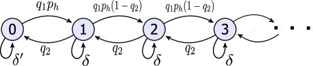
Figure 3: Markov chain model of the battery queue given that the data queues $Q_{1}$ and $Q_{2}$ are backlogged. Note that $\delta^{\prime}\!=\!1\!-\!q_{1}p_{h}\!-q_{2}$ and $\delta\!=\!1\!-\!q_{1}p_{h}(1-q_{2})\!-q_{2}$.

IV Main Results

In this section, we present our main results pertaining to the stable throughput region of the opportunistic RF energy harvesting slotted Aloha network $\mathcal{S}_{G}$. We adopt the notion of stability proposed in [25], where the stability of a queue is determined by the existence of a proper limiting distribution. A queue is said to be stable if

$$\lim_{t\rightarrow\infty}\mathbb{P}[Q^{t}<x]=F(x)\textit{ and }\lim_{x\rightarrow\infty}F(x)=1.$$ (14)

The stability of a queue is equivalent to the recurrence of the Markov chain modeling the queue length. Loynes’ Theorem [32] states that if the arrival and service processes of a queue are strictly jointly stationary and the average arrival rate is less than the average service rate, then the queue is stable. Also, if the average arrival rate is greater than the average service rate, then the queue is unstable and the queue size $Q^{t}$ approaches infinity almost surely. The stable throughput region of a system is defined as the set of arrival rate vectors, $(\lambda_{1},\lambda_{2})$ for our system, for which all data queues in the system are stable.
Next, we establish sufficient conditions on the stability of the opportunistic RF energy harvesting Aloha $\mathcal{S}_{G}$. Assuming half-duplex energy harvesting and unlimited battery capacity, the stability region is characterized by the following theorem.
Theorem 1. An inner bound on the stable throughput region of the opportunistic RF energy harvesting slotted Aloha $\mathcal{S}_{G}$ is the triangle OBD, shown in Fig. 4. Assuming half-duplex energy harvesting and unlimited battery size, the region is characterized by

$$\mathbb{R}_{G}^{\text{inner}}=\bigg{\{}(\lambda_{1},\lambda_{2})\ \big{|}\ \lambda_{1}\leq q_{1}\left(1-\frac{\lambda_{2}}{1-q_{1}}\right),\lambda_{2}\leq\dfrac{(1-q_{1})\min\left\{\frac{q_{1}p_{h}}{(1+q_{1}p_{h})},q_{2}\right\}\lambda_{1}}{q_{1}\left(1-\min\left\{\frac{q_{1}p_{h}}{(1+q_{1}p_{h})},q_{2}\right\}\right)}\bigg{\}}.$$ (15)

Proof.

The proof is established in the Sections V-A to V-E. ∎

Theorem 2. The closure of the inner bound $\mathbb{R}_{G}^{\text{inner}}$ over all transmission probability vectors $\boldsymbol{q}=(q_{1},q_{2})$ is characterized by

$$\mathcal{C}_{(\mathbb{R}_{G}^{\text{inner}})}=\bigcup\limits_{\boldsymbol{q}}\ \mathbb{S}_{o}(\boldsymbol{q})=\bigg{\{}\!(\lambda_{1},\lambda_{2})\ \big{|}\lambda_{2}\leq\frac{p_{h}\lambda_{1}}{2}\!\left(1\!-\!\lambda_{1}\!+\!\lambda_{2}\!+\!\sqrt{(1\!+\!\lambda_{1}\!-\!\lambda_{2})^{2}\!-\!4\lambda_{1}}\right)\!\!\bigg{\}}.$$ (16)

Proof.

The proof is established in Section V-F. ∎

V Stability Analysis

For the majority of prior work on stability analysis of interacting queues, the service rate of a typical node decreases with respect to the transmissions of other nodes in the system. Perhaps, the most basic example is the conventional slotted Aloha system [21], where increasing the service rate of an arbitrary node comes at the expense of decreasing the service rate of other nodes. For our purposes, we refer to such systems without energy limitations as “interference-limited” systems.
On the other hand, in our RF energy harvesting system, transmissions from interfering nodes give rise to two opposing effects on Type II (RF energy harvesting) nodes. Similar to classic interference-limited systems, the interfering nodes create collisions and, thus, decrease the service rate of RF energy harvesting nodes. Meanwhile, transmissions from interfering nodes are exploited by RF energy harvesting nodes to opportunistically replenish their batteries. Therefore, from the perspective of an RF energy harvesting node, a fundamental trade-off prevails between the increased number of energy harvesting opportunities and the increased collision rate, which are both caused by interference. As will be shown formally, this fundamental trade-off splits the stable throughput region for RF energy harvesting slotted Aloha networks into two sub-regions, a sub-region where interference is advantageous for the RF energy harvesting node and another sub-region where it is not. These two sub-regions map directly to two modes of operation for our system and are characterized as follows:

1. Energy-limited mode: is the sub-region of the stable throughput region in which the transmissions of interfering nodes enhance the throughput of the RF energy harvesting node, i̇.e, the throughput enhancement due to the increased harvesting opportunities outweights the degradation due to collisions created by the interfering nodes.

2. Interference-limited mode: is the sub-region of the stable throughput region in which the transmissions of interfering nodes do not increase the throughput of the RF energy harvesting node, i̇.e, the throughput degradation due to collisions equals or outweighs the throughput increase due to the increased energy harvesting opportunities.

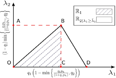
Figure 4: The energy limited and interference limited sub-regions of the stable throughput region of $\mathcal{S}_{D}$ are characterized by the triangles BCO and BCD, respectively.

The two parts of the stable throughput region for our system are shown in Fig. 4, where the energy-limited region is enclosed by the triangle BCO and the interference-limited region is enclosed by the triangle BCD.
In order to characterize the inner bound on the stability region of $\mathcal{S}_{G}$ in Theorem 1, we introduce a deprived system $\mathcal{S}_{D}$ where Type II node transmits only in the time slots in which $Q_{1}$ is non-empty. We derive the stability region of $\mathcal{S}_{D}$, by going through the following three steps discussed next. First, we characterize the average service rates of the two interacting data queues. Second, we generalize the Stochastic dominance technique proposed in [21] to capture our system dynamics and two-mode operation. Third, we derive the stability conditions of $\mathcal{S}_{D}$ using the generalized stochastic dominance approach. Finally, we prove in Section V-E that the stability region of $\mathcal{S}_{D}$ is an inner bound on the stability region of $\mathcal{S}_{G}$.

V-A Service Rates of the Interacting Queues in $\mathcal{S}_{G}$

The average service rates of the data queues, $Q_{1}$ and $Q_{2}$, in $\mathcal{S}_{G}$ are given by

$$\mu_{1} =q_{1}\big{(}1-q_{2}\ \mathbb{P}[B\!>\!0,Q_{2}\!>\!0|Q_{1}\!>\!0]\big{)},$$ (17)

$$\mu_{2} =q_{2}\ \mathbb{P}[B\!>\!0,Q_{1}\!=\!0|Q_{2}\!>\!0]+q_{2}\left(1-q_{1}\right)\ \mathbb{P}[B\!>\!0,Q_{1}\!>\!0|Q_{2}\!>\!0].$$ (18)

where the service rate of the Type I node, $\mu_{1}$, is the fraction of time in which Type I node decides to transmit, excluding the fraction of time in which Type II node is also transmitting. A Type II node transmits, if it is active, i̇.e., $B\!>\!0$ and $Q_{2}\!>\!0$, and decides to transmit. Similarly, the service rate of the Type II node, $\mu_{2}$, is the fraction of time in which Type II node has a non-empty battery and decides to transmit, excluding the fraction of time in which both nodes are transmitting. Note that the queue evolution equation in (1) implies that $\mathbb{P}[Q_{1}>0]=1$ in (17) and $\mathbb{P}[Q_{2}>0]=1$ in (18).

In our system, we have three interacting queues, namely $Q_{1}$, $Q_{2}$ and $B$. The analysis of three interacting queues is prohibitive and, hence, calculating the probability $\mathbb{P}[B\!>\!0,Q_{1}\!=\!0|Q_{2}\!>\!0]$. Therefore, we consider a system $\mathcal{S}_{D}$ where $\mathbb{P}[B\!>\!0,Q_{1}\!=\!0|Q_{2}\!>\!0]\!=\!0$, i̇.e., we consider a lower service rate for the Type II node, since it transmits only in the time slots in which $Q_{1}$ is non-empty. The relationship between the two systems is discussed in Section V-E.

V-B Service Rates of the Interacting Queues in $\mathcal{S}_{D}$

In order to analyze the interaction between $Q_{1}$ and $Q_{2}$ in $\mathcal{S}_{D}$, we decouple the battery queue, $B$, by substituting the probability of the battery queue being non-empty with the conditional probability given by Lemma 2. Hence, the average service rates of the data queues $Q_{1}$ and $Q_{2}$ are given as

$$\mu_{1} =q_{1}\big{(}1-q_{2}\ \mathbb{P}[B\!>\!0|Q_{1}\!>\!0,Q_{2}\!>\!0]\ \mathbb{P}[Q_{2}\!>\!0|Q_{1}\!>\!0]\big{)}$$ (19)

$$=q_{1}\big{(}1-\min\big{\{}\frac{q_{1}p_{h}}{(1+q_{1}p_{h})},q_{2}\big{\}}\ \mathbb{P}[Q_{2}\!>\!0|Q_{1}\!>\!0]\big{)}.$$ (20)

$$\mu_{2} =q_{2}\left(1-q_{1}\right)\mathbb{P}[B\!>\!0|Q_{1}\!>\!0,Q_{2}\!>\!0]\ \mathbb{P}[Q_{1}\!>\!0|Q_{2}\!>\!0]$$ (21)

$$=(1-q_{1})\min\big{\{}\frac{q_{1}p_{h}}{(1+q_{1}p_{h})},q_{2}\big{\}}\ \mathbb{P}[Q_{1}\!>\!0|Q_{2}\!>\!0].$$ (22)

The probability that $Q_{i}$ is non-empty given that $Q_{j}$ is saturated (always backlogged) is given by $\mathbb{P}[Q_{i}>0|Q_{j}>0]=\frac{\lambda_{i}}{\mu_{i}^{s}},\ i=1,2,\ i\neq j$, where $\mu_{i}^{s}$ is the service rate of $Q_{i}$ given that both data queues are saturated. We derive $\mu_{i}^{s},\ i=1,2$ in Section V-D.
From (20), we note that $\mu_{1}$ decreases with increasing $\mathbb{P}[Q_{2}>0|Q_{1}>0]$. Recall that for the interference-limited region, increasing the service rate of one node comes at the expense of decreasing the service rate of other nodes. The system is interference-limited from the perspective of Type I node, since increasing $\lambda_{2}$ comes at the expense of decreasing $\mu_{1}$. Also, from (22), we observe that $\mu_{2}$ is increasing in $\mathbb{P}[Q_{1}>0|Q_{2}>0]$. Hence, increasing $\lambda_{1}$ increases $\mu_{2}$ until both data queues are saturated. Thus, the system is energy-limited from the perspective of the Type II node until the data queues become saturated.

In Fig. 4, we depict the stable throughput region $\mathbb{R}_{D}$ of the system $\mathcal{S}_{D}$. The boundary between the energy-limited part and the interference limited part, from the perspective of the Type II node is $\lambda_{1}=\tilde{\lambda}_{1}$, where $\tilde{\lambda}_{1}$ is the arrival rate for $Q_{1}$ at which both data queues, $Q_{1}$ and $Q_{2}$, become saturated. Accordingly, the energy-limited sub-region is characterized by

$$\mathbb{R}_{D|\lambda_{1}\leq\tilde{\lambda}_{1}}=\big{\{}(\lambda_{1},\lambda_{2})\in\mathbb{R}_{D}|\ \lambda_{1}\leq\tilde{\lambda}_{1}\big{\}},$$ (23)

and the interference limited sub-region is characterized by

$$\mathbb{R}_{D|\lambda_{1}>\tilde{\lambda}_{1}}=\big{\{}(\lambda_{1},\lambda_{2})\in\mathbb{R}_{D}|\ \lambda_{1}>\tilde{\lambda}_{1}\big{\}}.$$ (24)

V-C The Generalized Stochastic Dominance Approach

In this section, we rely on stochastic dominance arguments [21], which are instrumental in establishing the stable throughput region of $\mathcal{S}_{D}$. However, the conventional stochastic dominance approach should be modified for our system, since the transmission of dummy packets by Type I node increases the harvesting opportunities for Type II node. Thus, in order to construct a hypothetical “dominant” system in which the queue lengths are never smaller than their counterparts in the system $\mathcal{S}_{D}$, the hypothetical system proposed in [21] is modified to capture the two-mode operation inherent to our RF EH system.
Recall, from (22), that the service rate of $Q_{2}$ increases with $\lambda_{1}$. Thus, it is straightforward to show that, using classic stochastic dominance arguments, saturating $Q_{1}$ increases the service rate of $Q_{2}$. Hence, the queue length in this hypothetical system (particularly $Q_{2}$) no longer dominates (i̇.e. could be smaller) its counterpart in the system $\mathcal{S}_{D}$ and, thus, the classic stochastic dominance argument fails. For example, if we consider the case where $\lambda_{1}=0$ and $\lambda_{2}>0$, we observe that $\lambda_{2}\leq q_{2}$ belongs to the stable throughput region, which contradicts (22), where for $\lambda_{1}=0$, we get $\lambda_{2}=0$.

Hence, we define the hypothetical system for our RF EH system to be constructed as follows:

• Arrivals at data queues $Q_{1}$ and $Q_{2}$ occur at the same instants as in the system $\mathcal{S}_{D}$.

• Transmission decisions, determined by independent coin tosses, are identical to those in the system $\mathcal{S}_{D}$.

• In the energy-limited region, Type I node does not transmit dummy packets. Thus, the energy arrivals to the battery queue of the harvesting node occurs exactly at the same instants as in the system $\mathcal{S}_{D}$.

• In the interference-limited region, if the data queue is empty and the node decides to transmit, a dummy packet is transmitted, if the node has sufficient energy to transmit.

From the construction of the new hypothetical system proposed above, it can be noticed that it behaves like the system $\mathcal{S}_{D}$ in the energy-limited region and dominates the system $\mathcal{S}_{D}$ in the interference-limited region. Thus, this hypothetical system dominates our system $\mathcal{S}_{D}$ because the transmissions of dummy packets collide with the transmission of the other node. Also, the transmissions of dummy packets consume energy without contributing to the throughput of Type II node.

V-D Establishing the Stability Conditions of $\mathcal{S}_{D}$

In order to derive the stability conditions of the system $\mathcal{S}_{D}$, we construct two dominant systems, where in the first dominant system Type II node is backlogged and in the second dominant system, Type I node is backlogged only in the interference-limited region.

V-D1 First dominant system

In this hypothetical system, we consider the case where the Type II node continues transmitting dummy packets whenever its data queue, $Q_{2}$, is empty given that its battery is non-empty. Since the system is interference-limited from the perspective of Type I node, our dominant system is identical to the one proposed in [21]. Hence, the saturated service rate of $Q_{1}$ is given by

$$\mu_{1}^{s}=q_{1}\big{(}1-\min\big{\{}\frac{q_{1}p_{h}}{(1+q_{1}p_{h})},q_{2}\big{\}}\big{)}.$$ (25)

Also, by substituting $\mathbb{P}[Q_{1}>0|Q_{2}>0]=\lambda_{1}/\mu_{1}^{s}$ in (22), the service rate of $Q_{2}$ becomes

$$\mu_{2}=\dfrac{(1-q_{1})\min\big{\{}\frac{q_{1}p_{h}}{(1+q_{1}p_{h})},q_{2}\big{\}}\lambda_{1}}{q_{1}\left(1-\min\big{\{}\frac{q_{1}p_{h}}{(1+q_{1}p_{h})},q_{2}\big{\}}\right)}.$$ (26)

Therefore, the stable throughput region of the first dominant system $\mathbb{S}_{1}$ is given by

$$\mathbb{R}_{1}=\bigg{\{}(\lambda_{1},\lambda_{2})\ \big{|}\ \lambda_{1}\leq q_{1}\big{(}1-\min\big{\{}\frac{q_{1}p_{h}}{(1+q_{1}p_{h})},q_{2}\big{\}}\big{)},\ \lambda_{2}\leq\dfrac{(1-q_{1})\min\left\{\frac{q_{1}p_{h}}{(1+q_{1}p_{h})},q_{2}\right\}\lambda_{1}}{q_{1}\left(1-\min\left\{\frac{q_{1}p_{h}}{(1+q_{1}p_{h})},q_{2}\right\}\right)}\bigg{\}}.$$ (27)

Also, since the system becomes interference-limited from the perspective of node II, when the data queues, $Q_{1}$ and $Q_{2}$, are backlogged, $\tilde{\lambda}_{1}$ is given by

$$\tilde{\lambda}_{1}=\mu_{1}^{s}=q_{1}\left(1-\min\left\{\frac{q_{1}p_{h}}{(1+q_{1}p_{h})},q_{2}\right\}\right).$$ (28)

V-D2 Second dominant system

In this hypothetical system, $Q_{1}$ is backlogged only in the interference-limited region from the perspective of Type II node. In the interference-limited part of $\mathbb{R}_{2}$, the saturated service rate of $Q_{2}$ is given by

$$\mu_{2}^{s}=(1-q_{1})\min\left\{\frac{q_{1}p_{h}}{(1+q_{1}p_{h})},q_{2}\right\}.$$ (29)

Similarly, by substituting $\mathbb{P}[Q_{2}>0|Q_{1}>0]=\lambda_{2}/\mu_{2}^{s}$ in (20), we obtain

$$\mu_{1}=q_{1}\left(1-\frac{\lambda_{2}}{1-q_{1}}\right).$$ (30)

Therefore, the stable throughput region of the interference-limited part of the second dominant system is given by

$$\mathbb{R}_{2|\lambda_{1}\geq\tilde{\lambda}_{1}}=\big{\{}(\lambda_{1},\lambda_{2})\ |\ \tilde{\lambda}_{1}\leq\lambda_{1}\leq q_{1}\big{(}1-\frac{\lambda_{2}}{1-q_{1}}\big{)},\lambda_{2}\leq(1-q_{1})\min\big{\{}\frac{q_{1}p_{h}}{(1+q_{1}p_{h})},q_{2}\big{\}}\big{\}}.$$ (31)

The stable throughput regions of the dominant systems $\mathbb{R}_{1}$ and $\mathbb{R}_{2|\lambda_{1}\geq\tilde{\lambda}_{1}}$ are shown in Fig. 4.

V-D3 Stability region of the system $\mathcal{S}_{D}$

In the following lemma we derive the relationship between the stable throughput region of the dominant systems $\mathbb{R}_{1}$ and $\mathbb{R}_{2|\lambda_{1}\geq\tilde{\lambda}_{1}}$ and the original system $\mathbb{R}_{D}$.
Lemma 3. The stable throughput region $\mathbb{R}_{D}$ of the system $\mathcal{S}_{D}$ is given by the union of the stable throughput region of the first dominant system and the interference-limited part of the second dominant system, i̇.e., $\mathbb{R}_{D}=\mathbb{R}_{1}\cup\mathbb{R}_{2|\lambda_{1}\geq\tilde{\lambda}_{1}}.$

Proof.

The stable throughput region of the original system is the union of the two dominant systems, based on [21], i̇.e., $\mathbb{R}_{D}=\mathbb{R}_{1}\cup\mathbb{R}_{2}$. From the construction of the second dominant system, we know that the energy-limited region is identical to the original system, i̇.e., $\mathbb{R}_{2|\lambda_{1}<\tilde{\lambda}_{1}}=\mathbb{R}_{D|\lambda_{1}<\tilde{\lambda}_{1}}$. Hence, we have $\mathbb{R}_{2}=\mathbb{R}_{D|\lambda_{1}<\tilde{\lambda}_{1}}\cup\mathbb{R}_{2|\lambda_{1}\geq\tilde{\lambda}_{1}}$ and $\mathbb{R}_{D}=\mathbb{R}_{1}\cup\mathbb{R}_{D|\lambda_{1}<\tilde{\lambda}_{1}}\cup\mathbb{R}_{2|\lambda_{1}\geq\tilde{\lambda}_{1}}.$
Now, assume that the rate pair $(x_{1},x_{2})\in\mathbb{R}_{D|\lambda_{1}<\tilde{\lambda}_{1}}$. Hence, $x_{1}<\tilde{\lambda}_{1}$ and $x_{2}\leq\mu_{2}$. Since we achieve the maximum service rate for Type II node by backlogging $Q_{2}$, from (27) we obtain

$$x_{2}\leq\dfrac{(1-q_{1})\min\left\{\frac{q_{1}p_{h}}{(1+q_{1}p_{h})},q_{2}\right\}x_{1}}{q_{1}\left(1-\min\left\{\frac{q_{1}p_{h}}{(1+q_{1}p_{h})},q_{2}\right\}\right)}.$$ (32)

Therefore, the rate pair $(x_{1},x_{2})\in\mathbb{R}_{1}$ and $\mathbb{R}_{D|\lambda_{1}<\tilde{\lambda}_{1}}\subseteq\mathbb{R}_{1}$. ∎

Proposition 1. The stability region of the system $\mathcal{S}_{D}$ is given by

$$\mathbb{R}_{D}=\bigg{\{}(\lambda_{1},\lambda_{2})\ \big{|}\ \lambda_{1}\leq q_{1}\left(1-\frac{\lambda_{2}}{1-q_{1}}\right),\lambda_{2}\leq\dfrac{(1-q_{1})\min\left\{\frac{q_{1}p_{h}}{(1+q_{1}p_{h})},q_{2}\right\}\lambda_{1}}{q_{1}\left(1-\min\left\{\frac{q_{1}p_{h}}{(1+q_{1}p_{h})},q_{2}\right\}\right)}\bigg{\}}.$$ (33)

Proof.

For the purpose of the proof, we also define a conventional Aloha system with nodes with unlimited energy supplies, i.e., $\mathcal{S}_{\text{Aloha}}$. The outline of the proof is as follows

1. The generalized stochastic dominance approach proves the necessity of the stability conditions on $Q_{1}$ and $Q_{2}$ in (33). Meanwhile, it only proves the sufficiency of the stability conditions for $Q_{2}$.

2. The stability condition on $Q_{1}$ in $\mathcal{S}_{\text{Aloha}}$ is sufficient for stability of $Q_{1}$ in $\mathcal{S}_{D}$.

3. The stability condition on $Q_{1}$ is the same in both systems $\mathcal{S}_{\text{Aloha}}$ and $\mathcal{S}_{D}$.

4. From (ii) and (iii), we establish the sufficiency of the stability condition on $Q_{1}$ for $\mathcal{S}_{D}$.

The detailed proof is as follows

1. Recall that for systems with unlimited energy such as $\mathcal{S}_{\text{Aloha}}$, the sufficient and necessary stability conditions are given by the union of the stability regions of the two hypothetical systems in [21]. On the other hand, for a system with batteries the transmission of dummy packets in the hypothetical system wastes the energy of the nodes which limits the data transmissions in future slots. For instance, in a hypothetical system where the first node is backlogged, there may exist instants at which the first node is unable to transmit due to energy outage, while it is able to transmit in the original system. Hence, the second node in the hypothetical system may have a higher success rate compared to the original system, and the sample path dominance is violated. Consequently, the union of the stability conditions of two hypothetical systems is only a necessary condition for the stability of the original system [29]. In our paper, we arrived to (33) by applying the generalized stochastic dominance approach, in which the first dominant system is constructed such that Type II node continues transmitting dummy packets whenever its data queue, $Q_{2}$, is empty. The transmission of dummy packets from Type II node in this system wastes energy. Therefore, Type I node in this dominant system may have a better success rate compared to that of the system $\mathcal{S}_{D}$. Therefore, the generalized stochastic dominance approach only proves the necessity of the stability condition on $Q_{1}$ in (33). On the other hand, the stability condition on $Q_{2}$ is sufficient and necessary, since Type I node has unlimited energy and the previous argument only applies to nodes with batteries.

2. In $\mathcal{S}_{\text{Aloha}}$ the two contending nodes have unlimited energy, while in $\mathcal{S}_{D}$ the transmissions of the Type II node are constrained by the energy in the battery. Hence, the second contending node in $\mathcal{S}_{\text{Aloha}}$, transmits more frequently than a Type II node with the same transmission probability $q_{2}$ in $\mathcal{S}_{D}$. Consequently, there are more collisions in $\mathcal{S}_{\text{Aloha}}$ compared with those in $\mathcal{S}_{D}$ and the service rate of Type I node in $\mathcal{S}_{D}$ cannot be smaller than the service rate of the first contending node in $\mathcal{S}_{\text{Aloha}}$. Therefore, the stability condition on $Q_{1}$ in $\mathcal{S}_{\text{Aloha}}$ is sufficient for stability of $Q_{1}$ in $\mathcal{S}_{D}$.

3. In the stability analysis of $\mathcal{S}_{D}$, we proved that the stability condition on $Q_{1}$ is $\lambda_{1}\leq q_{1}\left(1-\frac{\lambda_{2}}{1-q_{1}}\right)$, which is identical to the stability condition on $Q_{1}$ in $\mathcal{S}_{\text{Aloha}}$ [21].

4. The sufficiency of the condition $\lambda_{1}\leq q_{1}\left(1-\frac{\lambda_{2}}{1-q_{1}}\right)$ for the stability of $Q_{1}$ in $\mathcal{S}_{D}$ follows from its sufficiency for $Q_{1}$ in $\mathcal{S}_{\text{Aloha}}$. Therefore, the stability conditions in (33) are necessary and sufficient conditions and the region $\mathbb{R}_{D}$ is the exact stability region of the system $\mathcal{S}_{D}$.

∎

V-E The Relationship between Stability Regions of $\mathcal{S}_{G}$ and $\mathcal{S}_{D}$

Lemma 4. The stability region of the system $\mathcal{S}_{D}$ is an inner bound on the stability region of the system $\mathcal{S}_{G}$, i.e., $\mathbb{R}_{G}\supseteq\mathbb{R}_{D}$.

Proof.

According to the assumption $\mathbb{P}[B\!>\!0,Q_{1}\!=\!0|Q_{2}\!>\!0]\!=\!0$ in the system $\mathcal{S}_{D}$, a Type II node has a lower service rate compared to a Type II node in the system $\mathcal{S}_{G}$. Hence, the length of $Q_{2}$ in the system $\mathcal{S}_{D}$ is never smaller than its counterpart in the system $\mathcal{S}_{G}$, i.e., the system $\mathcal{S}_{D}$ dominates $\mathcal{S}_{G}$ from the perspective of Type II node. Consequently, the stability of $Q_{2}$ in $\mathcal{S}_{D}$, is sufficient for the stability of $Q_{2}$ in $\mathcal{S}_{G}$. Additionally, the assumption $\mathbb{P}[B\!>\!0,Q_{1}\!=\!0|Q_{2}\!>\!0]\!=\!0$, implies that Type II node is not transmitting in the time slots at which $Q_{1}$ is empty. Hence, the number of idle slots increases, since at those time slots Type I node has no data packets to transmit. Accordingly, the service rate of Type I node is not affected, and the stability condition on $Q_{1}$ is the same in $\mathcal{S}_{D}$ and $\mathcal{S}_{G}$. We conclude that the stability region of $\mathcal{S}_{D}$ is an inner bound on the stability region of $\mathcal{S}_{G}$. ∎

Finally, from Proposition 1 and Lemma 4 we arrive to Theorem 1.

V-F The Closure over all Transmission Probabilities

In this subsection, we prove Theorem 2. The closure of the inner bound $\mathbb{R}_{G}^{\text{inner}}$, is defined by the union of all stability regions for a given $(q_{1},q_{2})$, i̇.e., $\mathcal{C}_{(\mathbb{R}_{G}^{\text{inner}})}=\bigcup\limits_{(q_{1},q_{2})}\ \mathbb{R}_{G}^{\text{inner}}((q_{1},q_{2})).$ In $\mathbb{R}_{G}^{\text{inner}}$, the service rate of Type II node is always lower than the arrival rate of Type I node, i̇.e., $\mu_{2}<\lambda_{1}$. Also, from (15), we note that $\mu_{2}$ is increasing in $\min\{\frac{q_{1}p_{h}}{(1+q_{1}p_{h})},q_{2}\}$, while $\mu_{1}$ is not affected by $q_{2}$. Hence, in order to find the closure $\mathcal{C}_{(\mathbb{R}_{G}^{\text{inner}})}$, we need to find $q_{2}$ that maximizes $\mu_{2}$. From (15), we observe that for maximizing $\mu_{2}$, the transmission probability of Type II node $q_{2}$ should be greater than or equal to $q_{2}^{*}=(q_{1}p_{h})/(1+q_{1}p_{h})$. Also, increasing $q_{2}$ beyond $q_{2}^{*}$ does not affect the service rate $\mu_{2}$.
Interestingly, we can interpret $q_{2}^{*}$ using Renewal reward theorem [33]. Assume that the data queues are backlogged and Type II node transmits whenever it receives an energy packet, i̇.e., $q_{2}=1$. Let the expected reward $R$ that Type II node obtains, be the transmission of one data packet, i̇.e., $\mathbb{E}[R]=1$. Also, the expected number of time slots, $T$, needed for the transmission of one data packet is one slot for transmission, and $(q_{1}p_{h})^{-1}$ slots are needed for harvesting one energy packet. Hence, the expected time needed for a transmission $\mathbb{E}[T]=1+(q_{1}p_{h})^{-1}$. Using the renewal reward theorem, we find that the effective transmission rate of Type II node is given by $q_{2,\textit{eff}}=\frac{\mathbb{E}[R]}{\mathbb{E}[T]}=\frac{q_{1}p_{h}}{1+q_{1}p_{h}}.$ Therefore, the previous expression represents the maximum possible transmission rate of Type II node, which is the minimum transmission probability $q_{2}$ that maximizes $\mu_{2}$. Now, the problem of finding the closure $\mathcal{C}_{(\mathbb{S}_{o})}$, reduces to finding the closure of $\mathbb{R}_{G}^{\text{inner}}((q_{1},q_{2}^{*}))$ over all $q_{1}$, i̇.e., $\mathcal{C}_{(\mathbb{R}_{G}^{\text{inner}})}=\bigcup\limits_{q_{1}\in[0,1]}\ \mathbb{R}_{G}^{\text{inner}}((q_{1},q_{2}^{*})),$ where

$$\mathbb{R}_{G}^{\text{inner}}((q_{1},q_{2}^{*}))=\big{\{}(\lambda_{1},\lambda_{2})\big{|}\ \lambda_{1}\leq q_{1}\big{(}1-\frac{\lambda_{2}}{1-q_{1}}\big{)},\lambda_{2}\leq(1-q_{1})p_{h}\lambda_{1}\big{\}},$$ (34)

which represents the triangle OBD in Fig. 6, where $\textit{D}\!=\!(q_{1},0)$, and $\textit{B}\!=\!\left(\frac{q_{1}}{1+q_{1}p_{h}},\frac{q_{1}p_{h}(1-q_{1})}{1+q_{1}p_{h}}\right)\!.$ Since, we know that the region $\mathbb{R}_{G}^{\text{inner}}$ consist of two line segments, the closure $\mathcal{C}_{(\mathbb{R}_{G}^{\text{inner}})}$ can be found be taking the union of the closures of the line segments $\overline{\textit{OB}}$, $\overline{\textit{BD}}$. First, we find the closure of the line segment $\overline{\textit{OB}}$ by solving $x=\frac{q_{1}}{1+q_{1}p_{h}}$, and $y=\frac{q_{1}p_{h}(1-q_{1})}{1+q_{1}p_{h}}$. The solution represents the trace of the point B for $q_{1}\in[0,1]$, which is $y=p_{h}x(1-\frac{x}{1-p_{h}x})$. Hence, the closure of $\overline{\textit{OB}}$ is given by

$$\mathcal{C}_{\overline{\textit{OB}}}=\big{\{}(\lambda_{1},\lambda_{2})\big{|}\ \lambda_{2}\leq\lambda_{1}p_{h}\big{(}1-\frac{\lambda_{1}}{1-\lambda_{1}p_{h}}\big{)}\big{\}},$$ (35)

which is represented in Fig. 5 by $\mathcal{C}_{\textit{OB}}^{1}$ and $\mathcal{C}_{\textit{OB}}^{2}$. Note that $\mathcal{C}_{\overline{\textit{OB}}}$ is a convex region, since it is a hypograph of a concave function. Next, in order to find the closure of $\overline{\textit{BD}}$, we solve $\max\limits_{q_{1}\in[0,1]}\ \ q_{1}\big{(}1-\frac{\lambda_{2}}{1-q_{1}}\big{)}.$ The solution gives us the closure of the line segment extending $\overline{\textit{OB}}$ to the $\lambda_{2}$-axis, represented by $\mathcal{C}_{\textit{BD}}^{1}$ and $\mathcal{C}_{\textit{BD}}^{2}$ in Fig. 5. However, since we want the closure of $\overline{\textit{BD}}$ and not the extension, $\mathcal{C}_{\overline{\textit{BD}}}$ is limited from the left by the trace of the point B. Thus, the closure of $\overline{\textit{BD}}$ is the region bounded from the left by $\mathcal{C}_{\textit{OB}}^{2}$ and bounded by $\mathcal{C}_{\textit{BD}}^{1}$ from the right. It is characterized by

$$\mathcal{C}_{\overline{\textit{BD}}}=\big{\{}(\lambda_{1},\lambda_{2})\ \big{|}\ \sqrt{\lambda_{1}}+\sqrt{\lambda_{2}}\leq 1,\ \lambda_{1}\!>\!\dfrac{1\!+\!2p_{h}\!-\!\sqrt{1\!+\!4p_{h}}}{2p_{h}^{2}},\ \lambda_{2}\!>\!\lambda_{1}p_{h}\big{(}1\!-\!\frac{\lambda_{1}}{1\!-\!\lambda_{1}p_{h}}\big{)}\big{\}}.$$ (36)

Note that the second condition can be found by solving the two equations of $\mathcal{C}_{\textit{OB}}^{2}$ and $\mathcal{C}_{\textit{BD}}^{1}$. Finally, the closure $\mathcal{C}_{(\mathbb{R}_{G}^{\text{inner}})}$ is the union of $\mathcal{C}_{\textit{OB}}$ and $\mathcal{C}_{\textit{BD}}$, which is represented by $\mathcal{C}_{\textit{OB}}^{1}$ and $\mathcal{C}_{\textit{BD}}^{1}$ in Fig. 5. After some algebraic manipulations, we obtain (16).
Remark: (16) can also be obtained by maximizing the service rate of Type II node $\mu_{2}$, subject to the stability condition of Type I node $\lambda_{1}\leq\mu_{1}$, i̇.e,

$$\max\limits_{q_{1}\in[0,1]}\ (1-q_{1})p_{h}\lambda_{1}\ \ \textit{s.t }\ \lambda_{1}\leq q_{1}\big{(}1-\frac{\lambda_{2}}{1-q_{1}}\big{)}.$$ (37)

Hence, the closure of our system is equivalent to maximizing $\mu_{2}$, because $\mu_{2}$ is upper bounded by $\mu_{1}$. Thus, by maximizing $\mu_{2}$, we implicitly maximize $\mu_{1}$.

Figure 5: The closure $\mathcal{C}_{(\mathbb{R}_{G}^{\text{inner}})}=\mathcal{C}_{\textit{OB}}^{1}\cup\mathcal{C}_{\textit{BD}}^{1}$, for $p_{h}=0.2$.

VI Model Extensions

In this section, we discuss two extensions to the previous stability analysis. First, we investigate the impact of having a finite capacity battery on the stable throughput region. Second, we investigate the effect of having a full-duplex RF energy harvesting node.

VI-A Finite Capacity Battery

In this subsection, we investigate the impact of having a finite capacity battery on the stable throughput region obtained in Theorem 1. Let $M$ be the capacity of Type II node battery. Thus, the battery evolution equation becomes

$$B^{t+1}=\min\left\{B^{t}-\mu_{B}^{t}+H^{t},M\right\}$$ (38)

Similar to the unlimited battery capacity case, the battery queue forms a decoupled discrete time Markov chain given that the data queues are backlogged. By analyzing the Markov chain we find the probability that the battery queue is non-empty.
Lemma 5. For a half-duplex RF energy harvesting node with battery of size $M$, the probability that the battery is non-empty, $\zeta$, given the data queues $Q_{1}$ and $Q_{2}$ are backlogged, is given by

$$\zeta=\begin{cases}\rho\left(\frac{1-\left(\frac{q_{1}p_{h}(1-q_{2})}{q_{2}}\right)^{M}}{1-\rho\left(\frac{q_{1}p_{h}(1-q_{2})}{q_{2}}\right)^{M}}\right),\ q_{2}\neq\frac{q_{1}p_{h}}{1+q_{1}p_{h}},\\ 1,\ q_{2}=\frac{q_{1}p_{h}}{1+q_{1}p_{h}}\end{cases}$$ (39)

where $\rho=\frac{q_{1}p_{h}}{q_{2}(1+q_{1}p_{h})}$ is the probability that the battery is non-empty in the infinite capacity battery case.

Proof.

Along the lines of Lemma 2. ∎

Next, we apply the same procedure used in proving the stability region for the infinite battery capacity case.
Corollary 1. An inner bound on the stable throughput region of the opportunistic RF energy harvesting slotted Aloha is the triangle OED, shown in Fig .6. Assuming half-duplex energy harvesting and a battery of size $M$, the region is characterized by the following equation

$$\mathbb{R}_{G}^{\text{inner}}=\left\{(\lambda_{1},\lambda_{2})|\ \lambda_{1}\leq q_{1}\left(1-\frac{\lambda_{2}}{1-q_{1}}\right),\lambda_{2}\leq\dfrac{q_{2}(1-q_{1})\zeta\lambda_{1}}{q_{1}\left(1-q_{2}\zeta\right)}\right\}$$ (40)

Proof.

Along the lines of Theorem 1. ∎

The reduction in the stability region due to finite capacity battery is the triangle OEB shown in Fig. 6.

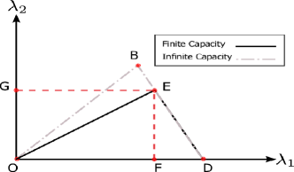
Figure 6: The stable throughput region of opportunistic energy harvesting Aloha with finite capacity battery is characterized by the triangle OED.

VI-B Full-Duplex Energy Harvesting

Now, we investigate the effect of having a full-duplex RF energy harvesting Type II node, i̇.e., the harvesting circuit is separated form the transmission circuit. Hence, a node can transmit and harvest simultaneously. Also, full-duplex energy transmission is advantageous because harvesting self-interference may introduce high energy yield. In the full-duplex RF energy harvesting paradigm, we have three types of harvesting opportunities. First, harvesting the transmissions of Type I node while Type II node is silent. Similar to the half-duplex case, we model this case by a Bernoulli process with mean $p_{h|\{1\}}$. Second, harvesting the self-interference of Type II node while Type I node is silent, which is modeled by a Bernoulli process with mean $p_{h|\{2\}}$. Third, harvesting both transmissions of Type I node and the self-interference of Type II node, which is modeled by a Bernoulli process with mean $p_{h|\{1,2\}}$.
In order to characterize the probabilities $p_{h|\{2\}}$ and $p_{h|\{1,2\}}$, we use a similar approach to the one used in characterizing $p_{h|\{1\}}$ in Section III. We assume that the loopback interference coefficient $c\in[0,1]$ is known [34]. Also, we assume a Rayleigh fading channel between the transmit antenna and the harvesting antenna, i̇.e., $g_{t}\sim\exp(1)$. In case only self-interference is present, the received power at time slot $t$ is equal to $P_{R}(t)=\eta P_{2}cg_{t}$. Hence, using the same approach as in the half-duplex case, we obtain

$$p_{h|\{2\}}=\frac{1}{1+\frac{\gamma}{\eta P_{2}c}}.$$ (41)

In case both transmissions of Type I node and the self-interference are present, the received power at time slot $t$ is equal to $P_{R}(t)=\eta(P_{1}h_{t}(1+l^{\alpha})^{-1}+\ P_{2}\ c\ g_{t})$. The probability $p_{h|\{1,2\}}$ can be characterized in a similar fashion.
For a full-duplex harvesting node, the average energy harvesting process of the battery queue is given by

$$\mathbb{E}[H^{t}] =q_{1}p_{h|\{1\}}\mathbb{P}[Q_{1}>0]+q_{2}p_{h|\{2\}}\mathbb{P}[Q_{1}=0,B>0,Q_{2}>0]$$ (42)

$$+(q_{2}p_{h|\{2\}}+q_{1}q_{2}(p_{h|\{1,2\}}-p_{h|\{2\}}-p_{h|\{1\}}))\mathbb{P}[Q_{1}>0,B>0,Q_{2}>0],$$

where $p_{h|\mathcal{M}},$ is the harvesting probability given a set $\mathcal{M}$ of nodes are transmitting. The battery queue forms a decoupled Markov chain given that the data queues are backlogged. By analyzing the Markov chain we find the probability that the battery is non-empty, which is given by the following lemma.
Lemma 6. For a full-duplex RF energy harvesting node with infinite capacity battery, the probability that the battery is non-empty $\Psi$, given the data queues $Q_{1}$ and $Q_{2}$ are backlogged, is given by

$$\Psi=\min\left\{\frac{q_{1}p_{h|\{1\}}}{q_{2}(1-q_{1}(p_{h|\{1,2\}}-p_{h|\{1\}})-(1-q_{1})p_{h|\{2\}})},1\right\}.$$ (43)

Proof.

Along the lines of Lemma 2. ∎

We notice that the probability of non-empty battery for the full-duplex case is higher than that of the half-duplex case, i̇.e, $\Psi\geq\frac{q_{1}p_{h|\{1\}}}{1+q_{1}p_{h|\{1\}}}.$ The stable throughput region of the system is given by
Corollary 2. An inner bound on the stable throughput region of the opportunistic RF energy harvesting slotted Aloha, under full-duplex energy harvesting mode and infinite capacity battery, is the region characterized by

$$\mathbb{R}_{G}^{\text{inner}}=\left\{(\lambda_{1},\lambda_{2})|\ \lambda_{1}\leq q_{1}\left(1-\frac{\lambda_{2}}{1-q_{1}}\right),\lambda_{2}\leq\dfrac{q_{2}(1-q_{1})\Psi\lambda_{1}}{q_{1}\left(1-q_{2}\Psi\right)}\right\}$$ (44)

Proof.

Along the lines of Theorem 1. ∎

VII Numerical Analysis

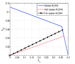
(a) $q_{2}>\Psi$.

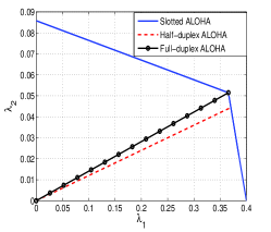
(b) $\frac{q_{1}p_{h|\{1\}}}{1+q_{1}p_{h|\{1\}}}<q_{2}<\Psi$.

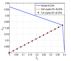
(c) $q_{2}<\frac{q_{1}p_{h|\{1\}}}{1+q_{1}p_{h|\{1\}}}$.

Figure 7: The stability regions of RF EH-Aloha under half/full-duplex modes vs. slotted Aloha with unlimited energy supply.

VII-A RF EH-Aloha System $\mathcal{S}_{G}$ Vs. Slotted Aloha

In Fig. 7, we compare the stable throughput region of the conventional slotted Aloha with unlimited energy supply with our RF EH-Aloha system $\mathcal{S}_{G}$. The stability regions are shown for $q_{1}=0.4$, $p_{h|\{1\}}=0.2$, $p_{h|\{2\}}=0.2$, and $p_{h|\{1,2\}}=0.35$. Also, we consider different values for $q_{2}$ to compare between full-duplex and half-duplex energy harvesting. We observe that the stability region of slotted Aloha is significantly reduced when RF energy harvesting is implemented, due to the energy limited sub-region. Also, for small $q_{2}$, i̇.e., $q_{2}<\frac{q_{1}p_{h|\{1\}}}{1+q_{1}p_{h|\{1\}}}$, we observe that the stability regions of half-duplex and full-duplex EH-Aloha are identical, because the service rate of Type II node is limited by the transmission probability $q_{2}$. On the other hand, for large $q_{2}$, i̇.e., $q_{2}>\Psi$, full-duplex RF energy harvesting expands the stability region, which agrees with intuition. From Fig. 7(a), we notice that increasing $q_{2}$ beyond $\Psi$ enhances the throughput of node $2$ in the slotted Aloha system. However, the throughput of the Type II node in full-duplex EH-Aloha is limited by $\Psi$.

VII-B Validating the Stability Conditions using Simulations

In Fig. 8 and 9, we simulate the energy harvesting Aloha system $\mathcal{S}_{D}$ for $q_{1}\!=\!0.4$, $q_{2}\!=\!0.4$, $p_{h}\!=\!0.6$ and the queues are averaged over $10^{5}$ time slots. In particular, Fig. 8 shows the sum of the average queue lengths $\mathbb{E}[Q_{1}^{t}]\!+\!\mathbb{E}[Q_{2}^{t}]$ versus the arrival rates $(\lambda_{1},\lambda_{2})$. We observed that the system exhibits unstable behavior, shown by the increase in the average queue lengths, as we cross the boundaries of the stability region. Fig. 9 shows the average service rate of $Q_{2}$ versus the arrival rates $(\lambda_{1},\lambda_{2})$. It shows that the maximum service rate (lower left corner points in the contour plot), for a given $\lambda_{2}$, is achieved on the boundary of the stability region. These observations support that $\mathbb{R}_{D}$ in Proposition 1 is indeed the stability region of $\mathcal{S}_{D}$.

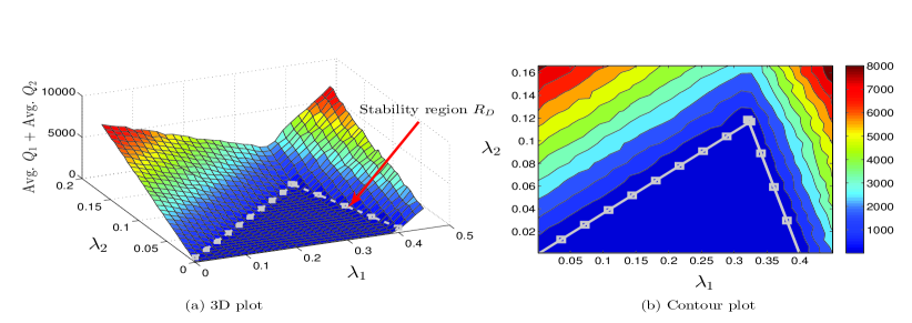
Figure 8: The stability regions $\mathbb{R}_{D}$ illustrated with the simulated sum average queue lenghts.

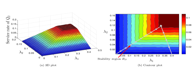
Figure 9: Simulation of the average service rate of $Q_{2}$ in system $\mathcal{S}_{D}$.

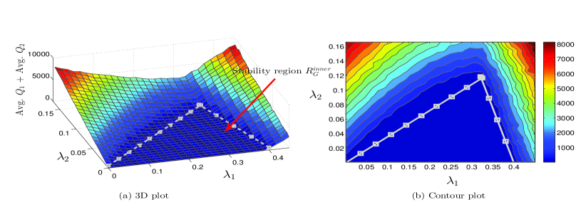
Figure 10: The stability region $\mathbb{R}_{G}^{\text{inner}}$ illustrated with the simulated sum average queue lenghts.

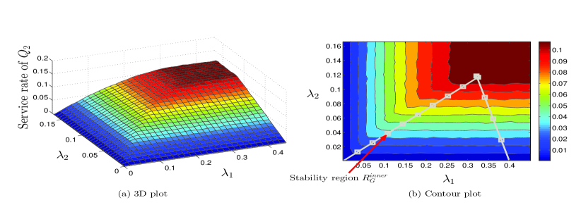
Figure 11: Simulation of the average service rate of $Q_{2}$ in system $\mathcal{S}_{G}$.

For the aforementioned parameters, we simulate the system $\mathcal{S}_{G}$ in order to verify the inner bound in Theorem 1. Similarly, the sum of the average queue lengths and the average service rate of $Q_{2}$ are shown in Fig. 10 and 11, respectively. We notice from Fig. 10 that there exist rate pairs outside the left hand side of the stability region for which the queues exhibit a stable behavior. Additionally, Fig. 11 suggests that the maximum service rate (lower left corner points in the contour plot), for a given $\lambda_{2}$, is achieved outside the stability region. These observations indicates that $\mathbb{R}_{G}^{\text{inner}}$ is an inner bound on the stability region of $\mathcal{S}_{G}$, as proposed in Theorem 1.
Finally, we show the utility of the stability region $\mathbb{R}_{G}^{\text{inner}}$, for the exact system $\mathcal{S}_{O}$ which is described in Section III-A. We simulate the exact behavior of the system for $\eta\!=\!0.7,\ \gamma\!=\!0.2335$, $P_{1}\!=\!1$ and $(1\!+\!l^{\alpha})^{-1}\!=\!0.5$. Hence, $\theta\!=\!0.667$ and from (9) we get $p_{h}\!=\!0.6$. The sum average queue lengths is shown in Fig. 12 versus the arrival rates $(\lambda_{1},\lambda_{2})$. We observe that the behavior of the average queue lengths in $\mathcal{S}_{O}$ is very similar to $\mathcal{S}_{G}$. Henceforth, we conjecture that the stability region $\mathbb{R}_{G}^{\text{inner}}$ is also an inner bound for the stability region of the exact system $\mathbb{R}_{O}$. To further support our analytical results, Fig. 13 and 14 present sample paths for the evolution of the queues $Q_{1}$ and $Q_{2}$ in the systems $\mathcal{S}_{D}$, $\mathcal{S}_{G}$ and $\mathcal{S}_{O}$. Note that the sample path of the evolution of an unstable queue should show an increasing tendency such that the queue size grow unboundedly as time increases. In Fig. 13, we show the evolution of $Q_{2}$ for two arrival rate pairs $T_{o}$ and $T_{i}$. We observe that $Q_{2}$ exhibits unstable behavior at $T_{o}$ in $\mathcal{S}_{D}$, while it exhibits stable behavior in $\mathcal{S}_{G}$ and $\mathcal{S}_{O}$. This supports our claim that the stability condition on $Q_{2}$ in (15) is sufficient and necessary in $\mathcal{S}_{D}$, while it is only sufficient in $\mathcal{S}_{G}$ and $\mathcal{S}_{O}$. While, Fig. 14 suggests that the stability condition on $Q_{1}$ in (15) is sufficient and necessary in $\mathcal{S}_{D}$, $\mathcal{S}_{G}$ and $\mathcal{S}_{O}$.

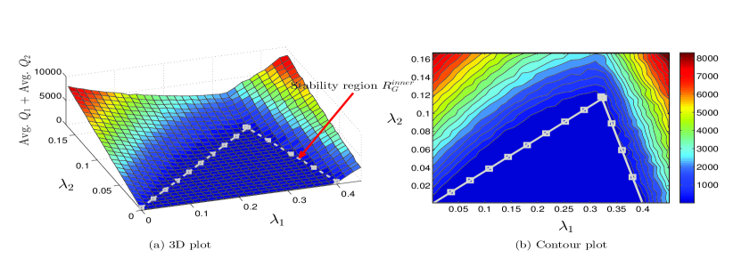
Figure 12: The stability region $\mathbb{R}_{G}^{\text{inner}}$ compared with the simulated sum average queue lenghts of the exact system $\mathcal{S}_{O}$.

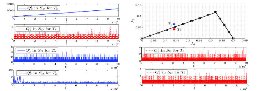
Figure 13: Sample paths for the evolution of $Q_{2}$ in the systems $\mathcal{S}_{D}$, $\mathcal{S}_{G}$ and $\mathcal{S}_{O}$.

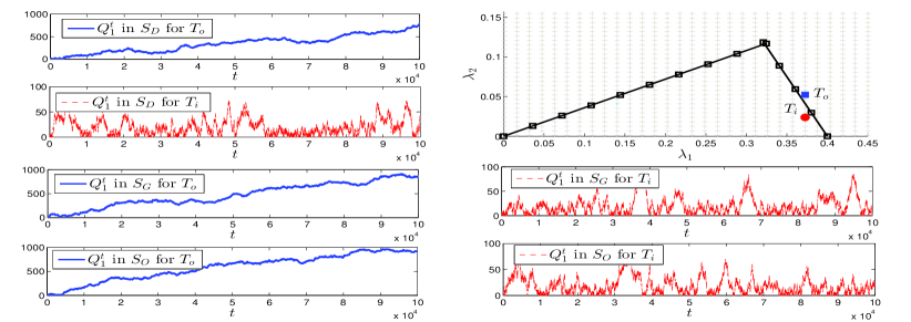
Figure 14: Sample paths for the evolution of $Q_{1}$ in the systems $\mathcal{S}_{D}$, $\mathcal{S}_{G}$ and $\mathcal{S}_{O}$.

VIII Conclusion

In this paper, we studied the effects of opportunistic RF energy harvesting on the stability of a slotted Aloha system consisting of a Type I node, which has unlimited energy supply, and a Type II node, which is solely powered by an RF energy harvesting circuit. We illustrated the intricacy in analyzing the exact behavior of such systems and proposed an equivalent system for which we were able to derive analytical results. In particular, we characterized an inner bound on the stability region under the half-duplex and full-duplex energy harvesting paradigms, by generalizing the stochastic dominance technique for RF EH-networks. We verified our analytical findings by simulating the exact and equivalent systems. The extension of our analysis to a random access network with multiple nodes can provide further insights to the development of efficient medium access protocols for networks with RF energy harvesting capabilities, and presents itself as a promising future research direction.

References

- [1] X. Lu, P. Wang, D. Niyato, and E. Hossain, “Dynamic spectrum access in cognitive radio networks with RF energy harvesting,” IEEE Wireless Communications, vol. 21, no. 3, pp. 102–110, 2014.
- [2] O. Ozel and S. Ulukus, “Achieving AWGN capacity under stochastic energy harvesting,” IEEE Transactions on Information Theory, vol. 58, no. 10, pp. 6471–6483, 2012.
- [3] D. Gunduz, K. Stamatiou, N. Michelusi, and M. Zorzi, “Designing intelligent energy harvesting communication systems,” IEEE Communications Magazine, vol. 52, no. 1, pp. 210–216, 2014.
- [4] J. Yang and S. Ulukus, “Optimal packet scheduling in an energy harvesting communication system,” IEEE Transactions on Communications, vol. 60, no. 1, pp. 220–230, 2012.
- [5] K. Tutuncuoglu and A. Yener, “Optimum transmission policies for battery limited energy harvesting nodes,” IEEE Transactions on Wireless Communications, vol. 11, no. 3, pp. 1180–1189, 2012.
- [6] O. Ozel, K. Tutuncuoglu, J. Yang, S. Ulukus, and A. Yener, “Transmission with energy harvesting nodes in fading wireless channels: Optimal policies,” IEEE Journal on Selected Areas in Communications, vol. 29, no. 8, pp. 1732–1743, 2011.
- [7] J. Yang, O. Ozel, and S. Ulukus, “Broadcasting with an energy harvesting rechargeable transmitter,” IEEE Transactions on Wireless Communications, vol. 11, no. 2, pp. 571–583, 2012.
- [8] J. Yang and S. Ulukus, “Optimal packet scheduling in a multiple access channel with energy harvesting transmitters,” Journal of Communications and Networks, vol. 14, no. 2, pp. 140–150, 2012.
- [9] K. Tutuncuoglu and A. Yener, “Sum-rate optimal power policies for energy harvesting transmitters in an interference channel,” Journal of Communications and Networks, vol. 14, no. 2, pp. 151–161, 2012.
- [10] B. Gurakan, O. Ozel, J. Yang, and S. Ulukus, “Energy cooperation in energy harvesting communications,” IEEE Transactions on Communications, vol. 61, no. 12, pp. 4884–4898, 2013.
- [11] L. R. Varshney, “Transporting information and energy simultaneously,” in International Symposium on Information Theory (ISIT). IEEE, 2008, pp. 1612–1616.
- [12] A. M. Fouladgar and O. Simeone, “On the transfer of information and energy in multi-user systems,” IEEE Communications Letters, vol. 16, no. 11, pp. 1733–1736, 2012.
- [13] X. Lu, P. Wang, D. Niyato, D. I. Kim, and Z. Han, “Wireless networks with RF energy harvesting: A contemporary survey,” IEEE Communications Surveys and Tutorials, vol. 17, no. 2, pp. 757–789, 2015.
- [14] R. Zhang and C. K. Ho, “MIMO broadcasting for simultaneous wireless information and power transfer,” in Global Telecommunications Conference (GLOBECOM). IEEE, 2011, pp. 1–5.
- [15] N. Abramson, “The Aloha system: another alternative for computer communications,” in Proceedings of the fall joint computer conference November 17-19. ACM, 1970, pp. 281–285.
- [16] H. Okada, Y. Igarashi, and Y. Nakanishi, “Analysis and application of framed Aloha channel in satellite packet switching networks-FADRA method,” Electronics Communications of Japan, vol. 60, pp. 72–80, 1977.
- [17] L. Zhu and T.-S. P. Yum, “A critical survey and analysis of RFID anti-collision mechanisms,” IEEE Communications Magazine, vol. 49, no. 5, pp. 214–221, 2011.
- [18] H. Wu, C. Zhu, R. J. La, X. Liu, and Y. Zhang, “FASA: Accelerated s-Aloha using access history for event-driven M2M communications,” IEEE/ACM Transactions on Networking, vol. 21, no. 6, pp. 1904–1917, 2013.
- [19] G. Fayolle and R. Iasnogorodski, “Two coupled processors: the reduction to a Riemann-Hilbert problem,” Zeitschrift für Wahrscheinlichkeitstheorie und verwandte Gebiete, vol. 47, no. 3, pp. 325–351, 1979.
- [20] B. S. Tsybakov and V. A. Mikhailov, “Ergodicity of a slotted Aloha system,” Problemy Peredachi Informatsii, vol. 15, no. 4, pp. 73–87, 1979.
- [21] R. R. Rao and A. Ephremides, “On the stability of interacting queues in a multiple-access system,” IEEE Transactions on Information Theory, vol. 34, no. 5, pp. 918–930, 1988.
- [22] W. Luo and A. Ephremides, “Stability of N interacting queues in random-access systems,” IEEE Transactions on Information Theory, vol. 45, no. 5, pp. 1579–1587, 1999.
- [23] C. Bordenave, D. McDonald, and A. Proutiere, “Asymptotic stability region of slotted Aloha,” IEEE Transactions on Information Theory, vol. 58, no. 9, pp. 5841–5855, 2012.
- [24] S. Kompalli and R. Mazumdar, “On the stability of finite queue slotted-Aloha protocol,” IEEE Transactions on Information Theory, vol. 59, no. 10, pp. 6357–6366, 2013.
- [25] W. Szpankowski, “Stability conditions for some distributed systems: Buffered random access systems,” Advances in Applied Probability, pp. 498–515, 1994.
- [26] S. Ghez, S. Verdu, and S. C. Schwartz, “Stability properties of slotted Aloha with multipacket reception capability,” IEEE Transactions on Automatic Control, vol. 33, no. 7, pp. 640–649, 1988.
- [27] V. Naware, G. Mergen, and L. Tong, “Stability and delay of finite-user slotted Aloha with multipacket reception,” IEEE Transactions on Information Theory, vol. 51, no. 7, pp. 2636–2656, 2005.
- [28] J. Jeon and A. Ephremides, “The stability region of random multiple access under stochastic energy harvesting,” in International Symposium on Information Theory (ISIT). IEEE, 2011, pp. 1796–1800.
- [29] ——, “On the stability of random multiple access with stochastic energy harvesting,” IEEE Journal on Selected Areas in Communications, vol. 33, no. 3, pp. 571–584, 2015.
- [30] H. Inaltekin, M. Chiang, H. V. Poor, and S. B. Wicker, “On unbounded path-loss models: effects of singularity on wireless network performance,” IEEE Journal on Selected Areas in Communications, vol. 27, no. 7, pp. 1078–1092, 2009.
- [31] P. Coporation, “RF energy harvesting and wireless power for low-power applications,” 2011.
- [32] R. Loynes, “The stability of a queue with non-independent inter-arrival and service times,” in Mathematical Proceedings of the Cambridge Philosophical Society, vol. 58, no. 03. Cambridge Univ Press, 1962, pp. 497–520.
- [33] S. M. Ross, Stochastic processes. John Wiley & Sons New York, 1996, vol. 2.
- [34] A. Thangaraj, R. K. Ganti, and S. Bhashyam, “Self-interference cancellation models for full-duplex wireless communications,” in International Conference on Signal Processing and Communications (SPCOM). IEEE, 2012, pp. 1–5.
- [35] C. A. Coelho, “The generalized integer Gamma distribution—a basis for distributions in multivariate statistics,” Journal of Multivariate Analysis, vol. 64, no. 1, pp. 86–102, 1998.