Cosmic evolution of scalar fields with multiple vacua: generalized DBI and quintessence

Abstract

We find a method to rewrite the equations of motion of scalar fields, generalized DBI field and quintessence, in the autonomous form forarbitrary scalar potentials. With the aid of this method, we explore the cosmic evolution of generalized DBI field and quintessence with the potential of multiple vacua. Then we find that the scalars are always frozen in the false or true vacuum in the end. Compared to the evolution of quintessence, the generalized DBI field has more times of oscillations around the vacuum of the potential. The reason for this point is that, with the increasing of speed $\dot{\phi}$, the friction term of generalized DBI field is greatly decreased. Thus the generalized DBI field acquires more times of oscillations.

I Introduction

Scalar fields play an important role in both theoretical physics and modern cosmology for their simple but non-trivial dynamics. In theoretical physics, they are present in the Jordan-Brans-Dicke theory as Jordan-Brans-Dicke scalar brans:61 ; in Kaluza-Klein compactification theory as the radion csaki:00 ; in the Standard Model of particle physics as the Higgs boson higgs:64 ; in the low-energy limit of the superstring theory as the dilaton gib:88 , tachyon sen:02 and DBI (Dirac-Born-Infeld) field ward:07 . In cosmology, scalar fields are employed to model the inflaton guth:81 , the quintessence fujii:88 ; ratra:88 ; chiba:97 ; fer:97 ; cope:98 ; cald:98 ; zla:99 (for a recent review of quintessence, see Refs. tsu:13 and references therein), the k-essence chiba:00 ; arm:00 , the phantom cald:02 , in order to drive the inflation of the early Universe or to speed up the expansion of the late Universe. We note that most of the scalar fields are hypothetical particles. But the Higgs Boson has uniquely been discovered by experiments.

Quintessence is a canonical scalar field which is assumed to be minimally coupled to gravity. Compared to other scalar fields, quintessence turns out to be the simplest scenario which is free of ghosts and instability problems. The dynamics of quintessence in the presence of matters has been studied in great detail for many different potentials cope:98 ; cald:98 ; zla:99 ; mac:00 ; ng:01 ; cor:03 ; cald:05 ; linder:06 ; bar:00 ; cope:09 ; liddle:99 ; sahni:00IJ ; sahni:00PRD . However, for a general quintessence potential, the equations of motion are rather involved. To our knowledge, one have not yet find a general method to write the equations of motion in the autonomous form for arbitrary potential. Thus the purpose of this article is to report that we have found a way.

The DBI field describes the dynamics of D-branes evolving in a higher-dimensional warped spacetime. A novel aspect of this field is the existence of a speed limit on the field space, resulting from causality restrictions on the motion of the branes in the bulk spacetime. The speed limit is enforced by the non-canonical kinetic terms in the DBI field. This is different from the quintessence whose speed $\nabla{\phi}$ could be arbitrarily large. From this point of view, quintessence and DBI field are the counterpart of Newtonian and Special Relativity mechanics, respectively. The cosmic evolution of DBI field have been studied in Refs. guo:08 . These researches only apply to some special forms of potentials. Thus, to find a general method applying to arbitrary DBI potential constitutes the second purpose of this article.

II generalized DBI field

We consider a $\textrm{D}3$-brane with tension T evolving in a 5-dimensional spacetime. The dynamics of the mobile D3-brane is described by the DBI action. The D3-brane is free to move on the internal compact Calabi-Yau manifold. The generalized DBI action can be written as follows ward:07

$$S = \int d^{4}x\sqrt{-g}\left[T\left(\psi\right)W\left(\psi\right)\sqrt{1+\frac{1}{T\left(\psi\right)}\partial_{\mu}\psi\partial^{\mu}\psi}\right.$$ (1)

$$\left.-T\left(\psi\right)+{V}\left(\psi\right)\right]+S_{m}\;.$$

Here $T(\psi)$ is the warped tension of the brane and $S_{m}$ is the action for matters localized in the D3-brane. The potential $W(\psi)$ could arise under the condition that the brane is a non-BPS one sen:02 or there are multiple coincident branes myers:99 . The potential ${V}(\psi)$ is related to the brane’s interactions with bulk fields or other branes.

In order to simplify our derivations, we define the variable $\phi$ as follows

$$\frac{1}{\sqrt{T\left(\psi\right)}}\partial_{\mu}\psi=\partial_{\mu}\phi\;.$$ (2)

Then above action can be written as

$$S = \int d^{4}x\sqrt{-g}\left[T\left(\phi\right)W\left(\phi\right)\sqrt{1+\partial_{\mu}\phi\partial^{\mu}\phi}\right.$$ (3)

$$\left.-T\left(\phi\right)+{V}\left(\phi\right)\right]+S_{m}\;.$$

Without the loss of physical significance, we could absorb the term $T(\phi)$ into $W(\phi)$ and $V(\phi)$, respectively. Then we find the action is simply

$$S = \int d^{4}x\sqrt{-g}\left[W\left(\phi\right)\sqrt{1+\partial_{\mu}\phi\partial^{\mu}\phi}+{V}\left(\phi\right)\right]+S_{m}\;.$$ (4)

We shall investigate the cosmic evolution of the DBI field in the background of spatially flat Friedmann-Robertson-Walker Universe

$$ds^{2}=-dt^{2}+a\left(t\right)^{2}\left(dr^{2}+r^{2}d\Omega^{2}\right)\;,$$ (5)

where $a(t)$ is the cosmic scale factor. We model the matter sources present in the Universe as perfect fluids. The perfect fluids can be baryonic matter, relativistic matter and dark energy. We assume there is no interaction between the generalized DBI scalar field and the matter fields, other than by gravity. Then the Einstein equations and the equation of motion of the scalar field are given

$$3H^{2}=\kappa^{2}\left(W\gamma+V+\rho_{m}\right)\;,$$

$$2\dot{H}+3H^{2}=-\kappa^{2}\left(-W/\gamma-V+\omega_{m}\rho_{m}\right)\;,$$ (6)

and

$$\ddot{\phi}+\frac{1}{\gamma^{2}}\cdot 3H\dot{\phi}+\frac{1}{\gamma^{3}}\cdot\frac{V_{,\phi}}{W}+\frac{1}{\gamma^{2}}\cdot\frac{W_{,\phi}}{W}=0\;,$$ (7)

respectively. Here $H\equiv\dot{a}/a$ denotes the Hubble parameter and dot is the derivative with respect to cosmic time, $t$. $\rho_{m}$ and $\omega_{m}$ are the energy density and the equation of state for the matter sources. We have $\omega_{m}=-1,\ 0,\ 1/3,\ +1$ for the cosmological constant, dust matter, relativistic matter and stiff matter, respectively. In this paper, we shall consider the case of dust matter, $\omega_{m}=0$. $V_{,\phi}$ and $W_{,\phi}$ denote the derivative with respect to $\phi$. $\gamma$ is defined by

$$\gamma=\frac{1}{\sqrt{1-\dot{\phi}^{2}}}\;,$$ (8)

which has the physical meaning of the generalized Lorentz factor. It is apparent the speed of scalar $\dot{\phi}$ is constrained to be smaller than the speed of light. This is remarkably different from the usual quintessence which could have arbitrary large speed in the sense of classical mechanics.

Observing Eqs. (II) and Eq. (7), we could absorb the constant $\kappa^{2}/3$ ($\kappa^{2}=8\pi$) into $W,V$ and $\rho_{m}$, respectively,

$$W\longrightarrow W\cdot\frac{3}{\kappa^{2}}\;,$$ (9)

$$V\longrightarrow V\cdot\frac{3}{\kappa^{2}}\;,$$ (10)

$$\rho_{m}\longrightarrow\rho_{m}\cdot\frac{3}{\kappa^{2}}\;.$$ (11)

Then above equations of motion turns out to be

$$H^{2}=W\gamma+V+\rho_{m}\;,$$ (12)

$$2\dot{H}/3+H^{2}=W/\gamma+V-\omega_{m}\rho_{m}\;,$$ (13)

$$\ddot{\phi}+\frac{1}{\gamma^{2}}\cdot 3H\dot{\phi}+\frac{1}{\gamma^{3}}\cdot\frac{V_{,\phi}}{W}+\frac{1}{\gamma^{2}}\cdot\frac{W_{,\phi}}{W}=0\;.$$ (14)

Given the scalar potential $W(\phi)$, $V(\phi)$ and the equation of state $\omega_{m}$, we are left with three variables, $a(t),\rho_{m}$ and the DBI field $\phi(t)$. Then we have three variables and three independent differential equations. So the system of equations is closed.

It is rather difficult to find the analytic solutions to the equations of motion (12-14). Hence in order to solve them numerically, we had better rewrite them in the autonomous form. To this end, we introduce the following dimensionless quantities

$$X\equiv\dot{\phi}\;,\ \ \ \ \ \ \ \ \ U\equiv\frac{{V_{,\phi}}}{W^{\frac{3}{2}}}\;,$$ (15)

$$Y\equiv\frac{\sqrt{W}}{H}\;,\ \ \ \ \ Q\equiv\frac{{W_{,\phi}}}{W^{\frac{3}{2}}}\;,$$ (16)

$$Z\equiv\frac{\sqrt{V}}{H}\;,\ \ \ \ \ \ \ S\equiv\frac{{V_{,\phi}}}{V^{\frac{3}{2}}}\;,$$ (17)

$$N\equiv\ln a\;.$$ (18)

We see $U,\ Q,\ S$ are the functions of DBI field, $\phi$. So they can be expressed as the function of $Y/Z$. Now we have only three variables, namely, $X,\ Y,\ Z$ and it is sufficient for us to derive the corresponding three independent differential equations. We remember that the system of equations of $X,\ Y\,Z$ are an autonomous system if and only if $U,\ Q,\ S$ are expressed as the functions of $X,\ Y,\ Z$. For simplicity, we assume

$$\frac{V}{W}=\phi^{2}\;.$$ (19)

We emphasize that one could in general assume ${V}/{W}=F(\phi)$ with $F(\phi)$ other simple functions, for example, $F(\phi)=\phi^{n},\ e^{\alpha\phi},\ \ln\phi$ and so on. Then we could obtain $\phi=\phi\ (V/W)=\phi\ (Z/Y)$ from this equation. Similarly, $U,\ Q,\ S$ could be expressed as the function of $Z/Y$.

Now with the aid of this assumption, we are able to write the Eqs. (12-14) in the autonomous form and deal with any scalar potential, $V(\phi)$ in the calculations. In this article, we shall focus on the scalar potential $V(\phi)$ with the expression of

$$V = V_{0}+\frac{V_{1}}{\phi^{6}}\left(\phi-a_{1}\right)\left(\phi-a_{2}\right)\left(\phi-a_{3}\right)$$ (20)

$$\cdot\left(\phi-a_{4}\right)\left(\phi-a_{5}\right)\left(\phi-a_{6}\right)\;,$$

where $V_{i}$ and $a_{i}$ are all positive constants. The reason for this choice of potential is that what we want to study is a potential with multiple vacua. Scalar fields with multiple vacua are very interesting because they have both theoretical origin in string landscape landscape:03 and theoretical study in Coleman-De Luccia tunnelling coleman:77 .

We note that the case of the well-known AdS throat, $W(\phi)=\lambda/\phi^{4}$ has been included in the desired one. As an example, we put $V_{0}=2,\ V_{1}=10^{4},\ a_{1}=1,\ a_{2}=11/10,\ a_{3}=9/8,\ a_{4}=39/25,\ a_{5}=157/100,\ a_{6}=2$ in the following discussions.

Name	$X$	$Y$	$Z$	$\phi$	Stability	$\Omega_{\phi}$	$w_{\phi}$
(a)	$0$	$0.70$	$0.72$	$\sigma_{1}=1.03$	Stable spiral (attractor)	$1$	$-1$
(b)	$0$	$0.67$	$0.74$	$\xi_{1}=1.11$	Saddle point	$1$	$-1$
(c)	$0$	$0.61$	$0.79$	$\sigma_{2}=1.31$	Stable spiral (attractor)	$1$	$-1$
(d)	$0$	$0.54$	$0.84$	$\xi_{2}=1.56$	Saddle point	$1$	$-1$
(e)	$0$	$0.47$	$0.88$	$\sigma_{3}=1.86$	Stable spiral (attractor)	$1$	$-1$

Table 1: Properties of the critical points for the scalar potential given by Eq. (20).

In Fig. 1, we plot the potential $V(\phi)$ with respect to $\phi$. There are two local maximum ($\xi_{1}=1.11,\ \xi_{2}=1.56$), one real vacuum ($\sigma_{3}=1.863$) and two false vacuum ($\sigma_{1}=1.029,\ \sigma_{2}=1.305$) for the potential. Physically, the scalar field would roll down the potential and then passes through the first ($\sigma_{1}$) and the second ($\sigma_{2}$) false vacuum. Finally, it arrives at the real vacuum ($\sigma_{3}$). The detail of the trajectory is closely related to the initial velocity, $\dot{\phi_{i}}$ (with the initial value, $\phi_{i}$ fixed). When the initial speed $\dot{\phi_{i}}$ is small enough, the scalar would acquire damped oscillations due to the Hubble friction in the first false vacuum and finally it is frozen in this vacuum. However, with the increasing of initial speed, the scalar could cross the first local maximum ($\xi_{1}$) and finally is frozen in the second false vacuum ($\sigma_{2}$). With even much larger initial velocity, the scalar could cross the two local maximum ($\xi_{1}$ and $\xi_{2}$) and finally dwells on the real vacuum ($\sigma_{3}$). Since the speed of the scalar is constrained to be smaller than the speed of light, the scalar can not climb the hill with arbitrary height. Due to the Hubble friction, we expect the fate of the scalar is to dwell on the real vacuum. In what follows, we shall show theses points numerically.

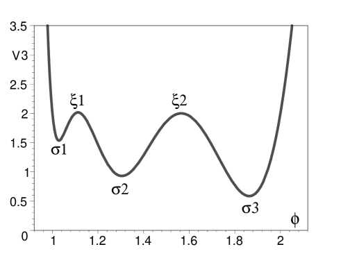
Figure 1: The DBI potential $V(\phi)$ with respect to $\phi$. There are two local maximum ($\xi_{1}=1.11,\ \xi_{2}=1.56$), one real vacuum ($\sigma_{3}=1.86$) and two false vacuum ($\sigma_{1}=1.03,\ \sigma_{2}=1.31$) for the potential. Physically, the scalar field would roll down the potential and then passes through the first ($\sigma_{1}$) and the second ($\sigma_{2}$) false vacuum. Finally, it arrives at the real vacuum ($\sigma_{3}$).

.

Using the dimensionless variables defined in (15-18), the equations of motion (12-14) can be written in the following autonomous form

$$\frac{dX}{dN} = -\frac{1}{\gamma^{2}}\cdot 3X-\frac{1}{\gamma^{3}}\cdot UY-\frac{1}{\gamma^{2}}\cdot QY\;,$$

$$\frac{dY}{dN} = \frac{1}{2}QXY^{2}-Y\frac{\dot{H}}{H^{2}}\;,$$

$$\frac{dZ}{dN} = \frac{1}{2}SXZ^{2}-Z\frac{\dot{H}}{H^{2}}\;,$$ (21)

where $U,\ Q,\ S$ are the functions of $Y/Z$ and

$$\gamma = \frac{1}{\sqrt{1-X^{2}}}\;,$$ (22)

$$\frac{\dot{H}}{H^{2}} = 3Y^{2}\cdot\frac{1-\gamma^{2}}{2\gamma}-\frac{3}{2}\left(1-\gamma Y^{2}-Z^{2}\right)\;.$$ (23)

The Friedmann equation becomes the constraint equation

$$1=\frac{Y^{2}}{\sqrt{1-X^{2}}}+Z^{2}+\frac{\rho_{m}}{H^{2}}\;.$$ (24)

The equation of state $w$ of the DBI scalar field is

$$w \equiv \frac{-1/\gamma-Z^{2}/Y^{2}}{\gamma+Z^{2}/Y^{2}}\;.$$ (25)

In Table I, we present the properties of the five fixed points for the scalar field. The points (a, c, e) correspond to the false vacua ($\sigma_{1},\ \sigma_{2}$) and real vacuum ($\sigma_{3}$). The three points are stable spirals. On these epoches, the scalar field behaves as a damping oscillator with the equation of state of firstly behaving as the dust matter and then oscillating approaching $-1$ (see Fig. (5)). The points (b, d,) correspond to the two local maximum ($\xi_{1},\ \xi_{2}$) and they are saddle points. On these points, the speed of the scalar field exactly vanishes and the DBI field acquires the equation of state of cosmological constant.

In Fig. (2-4), we plot the evolution of the speed, $\dot{\phi}$ of the generalized DBI field with $\phi$. We fix the initial values of $\dot{\phi}$, $\phi$ and $\rho_{m}/H^{2}$. By this way, the initial values of $Y$ and $Z$ are determined. Fig. (2) shows that when the initial speed $\dot{\phi_{i}}$ is small enough, the scalar would acquire damped oscillating due to the Hubble friction in the false vacuum ($\sigma_{1}$) and finally it is frozen in this vacuum. With the increasing of initial speed, the scalar crosses the first local maximum ($\xi_{1}$) and finally is frozen in the second false vacuum ($\sigma_{2}$) (see Fig. (3)). With even much larger initial velocity, the scalar crosses the two local maximum ($\xi_{1}$ and $\xi_{2}$) and finally dwells on the real vacuum ($\sigma_{3}$) (see Fig. (4)).

In Fig. (5), we plot the evolution of the equation of state $w$ of the generalized DBI field corresponding to Fig. (4). We see the generalized DBI field previously behaves as the dust matter and then oscillating approaches $-1$ after a sufficient long time. The reason for oscillating of $\omega$ can be understood as follows. Eq. (25) tells us when the speed of DBI field vanishes, the equation of state is $-1$. Fig. (4) shows there are many times for the vanishing of speed during the damped oscillating. Every time the generalized DBI field acquires vanishing velocity, its equation of state is $-1$.

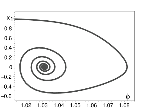
Figure 2: Evolution of the speed ($X=\dot{\phi}$) of generalized DBI field with $\phi$. The point $(\phi=\sigma_{1}=1.03,\ X=0)$ is a stable spiral and thus an attractor. In this case, the generalized DBI field behaves as a damping oscillator in the false vacuum ($\sigma_{1}$) and finally is frozen.

.

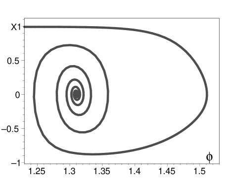
Figure 3: Evolution of the speed ($X=\dot{\phi}$) of generalized DBI field with $\phi$. The point $(\phi=\sigma_{2}=1.31,\ X=0)$ is a stable spiral and thus an attractor. In this case, the generalized DBI field behaves as a damping oscillator in the false vacuum ($\sigma_{2}$) and finally is frozen.

.

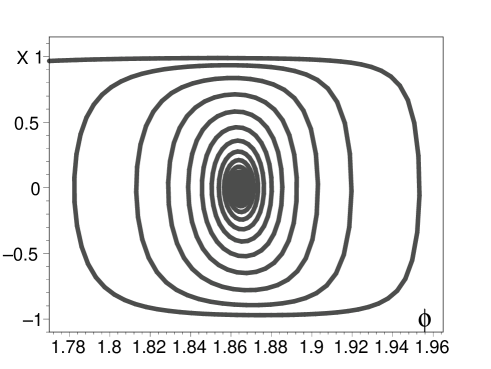
Figure 4: Evolution of the speed ($X=\dot{\phi}$) of generalized DBI field with $\phi$. The point $(\phi=\sigma_{2}=1.86,\ X=0)$ is a stable spiral and thus an attractor. In this case, the generalized DBI field behaves as a damping oscillator in the real vacuum ($\sigma_{3}$) and finally is frozen.

.

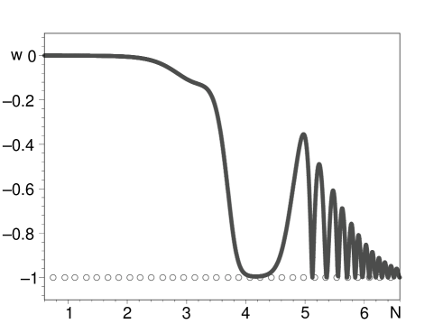
Figure 5: The evolution of the equation of state for the generalized DBI scalar field. It behaves as the dust matter at higher redshifts and oscillating approaches $-1$ at the lower redshifts

.

III quintessence

In this section, we shall present the method for dealing with arbitrary quintessence potential. As an example, we would explore the cosmic evolution of quintessence field with multiple vacua. To this end, let’s focus on the potential as follows

$$V=V_{0}e^{b\left(\phi-a_{1}\right)\left(\phi-a_{2}\right)\left(\phi-a_{3}\right)\left(\phi-a_{4}\right)\left(\phi-a_{5}\right)\left(\phi-a_{6}\right)}\;,$$ (26)

where $V_{0},\ b,\ a_{i}$ are positive constants. As an example, we consider, $V_{0}=1,\ b=1,\ a_{1}=1/2,\ a_{2}=3/5,\ a_{3}=1,\ a_{4}=17/10,\ a_{5}=2,\ a_{6}=5/2$.

In Fig. 6, we plot the potential $V(\phi)$ with respect to $\phi$. There are two local maximum ($\xi_{1}=0.813,\ \xi_{2}=1.862$), one real vacuum ($\sigma_{3}=2.342$) and two false vacuum ($\sigma_{1}=0.545,\ \sigma_{2}=1.355$) for the potential. Physically, the scalar field would roll down the potential and then damped oscillates between these vacua. Given an initial finite velocity $\dot{\phi}$ and field value $\phi_{0}$, the fate of the scalar is expected to dwell on the one of the vacuum due to the Hubble friction. In what follows, we shall show theses points numerically.

The Einstein equations and the equation of motion of the quintessence are given by

$$3H^{2}=\kappa^{2}\left(\frac{1}{2}\dot{\phi}^{2}+V+\rho_{m}\right)\;,$$

$$2\dot{H}+3H^{2}=-\kappa^{2}\left(\frac{1}{2}\dot{\phi}^{2}-V+\omega_{m}\rho_{m}\right)\;,$$ (27)

and

$$\ddot{\phi}+3H\dot{\phi}+V_{,\phi}=0\;,$$ (28)

respectively. Here $\rho_{m}$ and $\omega_{m}$ are the energy density and the equation of state for the matter sources. In this section, we also consider the case of dust matter, $\omega_{m}=0$.

Observing Eqs. (III) and Eq. (28), we could absorb the constant $\kappa^{2}/3$ ($\kappa^{2}=8\pi$) into $\phi^{2},V$ and $\rho_{m}$, respectively,

$$\phi^{2}\longrightarrow\phi^{2}\cdot\frac{6}{\kappa^{2}}\;,$$ (29)

$$V\longrightarrow V\cdot\frac{3}{\kappa^{2}}\;,$$ (30)

$$\rho_{m}\longrightarrow\rho_{m}\cdot\frac{3}{\kappa^{2}}\;.$$ (31)

Then above equations of motion turns out to be

$$H^{2}=\dot{\phi}^{2}+V+\rho_{m}\;,$$ (32)

$$2\dot{H}/3+H^{2}=-\dot{\phi}^{2}+V-\omega_{m}\rho_{m}\;,$$ (33)

$$\ddot{\phi}+3H\dot{\phi}+\frac{1}{2}{V_{,\phi}}=0\;.$$ (34)

Given the scalar potential $V(\phi)$ and the equation of state $\omega_{m}$, we are left with three variables, $a(t),\rho_{m}$ and the quintessence $\phi(t)$. Then we have three variables and three independent differential equations. So the system of equations is closed.

The same as the DBI case, it is rather involved to find the analytic solutions to the equations of motion (32-34). Hence in order to solve them numerically, we had better rewrite them in the autonomous form. To our knowledge, one have only explored some special form of the quintessence potential, namely, the exponential potential cope:98 ; ng:01 , power-law type potential ratra:88 ; cald:98 , the Albrecht and Skordis potential albrecht:99 an so on. For arbitrary potential, one have not yet find a general method to write the equations of motion in the autonomous form. In what follows, we shall propose a method that can be used to deal with arbitrary potentials.

To this end, we introduce the following dimensionless quantities

$$X\equiv\frac{\dot{\phi}}{H}\;,\ \ \ \ \ \ \ \ Q\equiv\frac{{V_{,\phi}}}{V}=Q\left(Z\right)\;,$$ (35)

$$Y\equiv\frac{\sqrt{V}}{H}\;,\ \ \ \ \ \ N\equiv\ln a\;,$$ (36)

$$Z\equiv\phi\;.\$$ (37)

With the aid of these definitions, we can write the equations of motion in the autonomous form with arbitrary potentials:

$$\frac{dX}{dN} = -3X-Y^{2}Q-X\cdot\frac{\dot{H}}{H^{2}}\;,$$

$$\frac{dY}{dN} = \frac{1}{2}XYQ-Y\frac{\dot{H}}{H^{2}}\;,$$

$$\frac{dZ}{dN} = X\;,$$ (38)

with

$$\frac{\dot{H}}{H^{2}} = -3X^{2}-\frac{3}{2}\left(1+\omega_{m}\right)\left(1-X^{2}-Y^{2}\right)\;.$$ (39)

We note that $Q$ is the function of $Z$. Therefore, Eqs. (III) is indeed an autonomous system of equations. In Table II, we present the properties of the five fixed points for the quintessence. The points (a, c, e) correspond to the false vacua ($\sigma_{1},\ \sigma_{2}$) and real vacuum ($\sigma_{3}$). The three points are stable spirals. On these epoches, the quintessence behaves as a damping oscillator with the equation of state of firstly behaving as the dust matter and then oscillating approaching $-1$. The points (b, d,) correspond to the two local maximum ($\xi_{1},\ \xi_{2}$) and they are saddle points. On these points, the speed of the scalar field exactly vanishes and the quintessence acquires the equation of state of cosmological constant.

Name	$X$	$Y$	$Z$	$\phi$	Stability	$\Omega_{\phi}$	$w_{\phi}$
(a)	$0$	$1$	$0.545$	$\sigma_{1}=0.545$	Stable spiral (attractor)	$1$	$-1$
(b)	$0$	$1$	$0.813$	$\xi_{1}=0.813$	Saddle point	$1$	$-1$
(c)	$0$	$1$	$1.355$	$\sigma_{2}=1.355$	Stable spiral (attractor)	$1$	$-1$
(d)	$0$	$1$	$1.862$	$\xi_{2}=1.862$	Saddle point	$1$	$-1$
(e)	$0$	$1$	$2.342$	$\sigma_{3}=2.342$	Stable spiral (attractor)	$1$	$-1$

Table 2: Properties of the critical points for the quintessence potential given by Eq. (26).

In Fig. (7-9), we plot the evolution of the rescaled speed, $X$ of the quintessence with $\phi$. The figures show that, with the increasing of initial speed, the quintessence is frozen in the first false vacuum, the second false vacuum and the real vacuum, respectively. Compared to evolution of DBI field, we see from Figs.(2-4) that the DBI field has more times of oscillations than quintessence. How to understand this point? The equations of motion tell us the friction term due to Hubble expansion is $3H\dot{\phi}$ and $3H\dot{\phi}\left(1-\dot{\phi}^{2}\right)$ for quintessence and DBI field, respectively. Then with the increasing of speed $\dot{\phi}$, the friction term of DBI field is greatly decreased. So the DBI field acquires more times of oscillations.

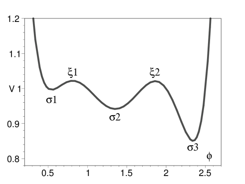
Figure 6: The quintessence potential $V(\phi)$ with respect to $\phi$. There are two local maximum ($\xi_{1}=0.813,\ \xi_{2}=1.862$), one real vacuum ($\sigma_{3}=2.342$) and two false vacuum ($\sigma_{1}=0.545,\ \sigma_{2}=1.355$) for the potential. Physically, the quintessence would firstly damped oscillates between these vacua and finally dwell on one of the vacuum due to the Hubble friction.

.

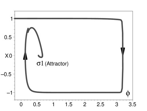
Figure 7: Evolution of the rescaled speed ($X$) of quintessence with $\phi$. The point $(\phi=\sigma_{1},\ X=0)$ is a stable spiral and thus an attractor. The quintessence is finally frozen at $\phi=\sigma_{1}$.

.

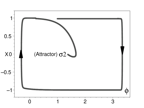
Figure 8: Evolution of the rescaled speed ($X$) of quintessence with $\phi$. The point $(\phi=\sigma_{2},\ X=0)$ is a stable spiral and thus an attractor. The quintessence is finally frozen at $\phi=\sigma_{2}$.

.

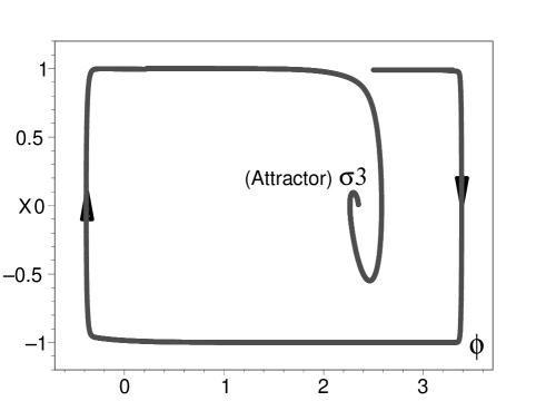
Figure 9: Evolution of the rescaled speed ($X$) of quintessence with $\phi$. The point $(\phi=\sigma_{3},\ X=0)$ is a stable spiral and thus an attractor. The quintessence is finally frozen at $\phi=\sigma_{3}$.

.

IV conclusion and discussion

In general, the equations of motion for generalized DBI field and quintessence are rather complicated. So one resort to the method of phase analysis by writing the equations of motion in the autonomous form. Many special form of potentials have been studied for DBI field guo:08 and quintessence cope:98 ; cald:98 ; zla:99 ; mac:00 ; ng:01 ; cor:03 ; cald:05 ; linder:06 ; bar:00 ; cope:09 ; liddle:99 ; sahni:00IJ ; sahni:00PRD . However, the general method for dealing with arbitrary potentials have not yet been proposed. Thus the outcome of this article is that we have found the method.

Different from the potentials studied in Refs. cope:98 ; cald:98 ; zla:99 ; mac:00 ; ng:01 ; cor:03 ; cald:05 ; linder:06 ; bar:00 ; cope:09 ; liddle:99 ; sahni:00IJ ; sahni:00PRD ; guo:08 , we investigate the cosmic evolution of the generalized DBI field and quintessence with the potential of multiple vacua. We find that, with the increasing of initial speed, both generalized DBI field and quintessence are successively frozen, in the first false vacuum, the second false vacuum and the real vacuum, respectively. Compared to the evolution of quintessence, the generalized DBI field has more times of oscillations. The reason for this point is that, with the increasing of speed $\dot{\phi}$, the friction term of generalized DBI field is greatly decreased. Thus the generalized DBI field acquires more times of oscillations.

The conclusion in this paper may be trivial, but the proof and the method are not. As an example, one could study the Coleman-De Luccia tunnelling using this method. After making the Wick rotation, $t=-i\tau$ in Eqs. (21) and Eqs. (38), we are able to study the Coleman-De Luccia tunnelling numerically but exactly.

- (1) C. Brans and R. H. Dicke, Phys. Rev. D 124, 925 (1961).
- (2) C. Csaki, M. Graesser, L. Randall, J. Terning, Phys. Rev. D 62, 045015 (2000).
- (3) P. W. Higgs, Phys. Lett. B 12, 132 (1964).
- (4) G. W. Gibbons, K. Maeda, Nucl. Phys. B 298, 741 (1988).
- (5) A. Sen, JHEP. 0204, 048 (2002).
- (6) S. Thomas and J. Ward, Phys. Rev. D 76, 023509 (2007) [arXiv:hep-th/0702229]; S. Thomas and J. Ward, JHEP. 0610, 039 (2006) [arXiv:hep-th/0508085].
- (7) A. H. Guth, Phys. Rev. D 23, 347 (1981).
- (8) Y. Fujii, Phys. Rev. D 26, 2580 (1982); L. H. Ford, Phys. Rev. D 35, 2339 (1987); C. Wetterich, Nucl. Phys. B 302, 668 (1988).
- (9) B. Ratra and P. J. E. Peebles, Phys. Rev. D 37, 3406 (1988).
- (10) T. Chiba, N. Sugiyama and T. Nakamura, Mon. Not. R. Astron. Soc. 289, L5 (1997).
- (11) P. G. Ferreira and M. Joyce, Phys. Rev. Lett. 79, 4740 (1997); Phys. Rev. D 58, 023503 (1998).
- (12) E. J. Copeland, A. R. Liddle and D. Wands, Phys. Rev. D 57, 4686 (1998).
- (13) R. R. Caldwell, R. Dave and P. J. Steinhardt, Phys. Rev. Lett. 80, 1582 (1998).
- (14) I. Zlatev, L. M. Wang and P. J. Steinhardt, Phys. Rev. Lett. 82, 896 (1999).
- (15) S. Tsujikawa, Class. Quant. Grav. 30, 214003 (2013).
- (16) T. Chiba, T. Okabe and M. Yamaguchi, Phys. Rev. D 62, 023511 (2000).
- (17) C. Armendariz-Picon, V. F. Mukhanov and P. J. Steinhardt, Phys. Rev. Lett. 85, 4438 (2000); Phys. Rev. D 63, 103510 (2001).
- (18) R. R. Caldwell, Phys. Lett. B 545, 23 (2002).
- (19) A. de la Macorra and G. Piccinelli, Phys. Rev. D 61, 123503 (2000).
- (20) S. C. C. Ng, N. J. Nunes and F. Rosati, Phys. Rev. D 64, 083510 (2001).
- (21) P. S. Corasaniti and E. J. Copeland, Phys. Rev. D 67, 063521 (2003).
- (22) R. R. Caldwell and E. V. Linder, Phys. Rev. Lett. 95, 141301 (2005).
- (23) E. V. Linder, Phys. Rev. D 73, 063010 (2006); E. Elizalde, A. N. Makarenko et al., Astrophys. Space. Sci. 344, 479 (2013).
- (24) T. Barreiro, E. J. Copeland and N. J. Nunes, Phys. Rev. D 61, 127301 (2000).
- (25) E. J. Copeland, S. Mizuno, M. Shaeri, Phys. Rev. D 79, 103515 (2009) [arXiv:0904.0877]; S. Nojiri, S. D. Odintsov, Phys. Lett. B 649, 440 (2007).
- (26) A. R. Liddle and R. J. Scherrer, Phys. Rev. D 59, 023509 (1999).
- (27) V. Sahni, A. Starobinsky, Int. J. Mod. Mod. Phys. D 9, 373 (2000); L. A. Urena-Lopez, T. Matos, Phys. Rev. D 62, 081302 (2000); S. A. Pavluchenko, Phys. Rev. D 67, 103518 (2003).
- (28) V. Sahni, L.-M. Wang, Phys. Rev. D 62, 103517 (2000) [astro-ph/9910097]; C. R. Fadragas, G. Leon, E. N. Saridakis, Class. Quant. Grav. 31, 075018 (2014).
- (29) Z. K. Guo and N. Ohta, JCAP. 0804, 035 (2008) [arXiv:0803.1013]; J. Martin and M. Yamaguchi, Phys. Rev. D 77, 123508 (2008); B. Gumjudpai and J. Ward, Phys. Rev. D 80, 023528 (2009); H. Wei, Phys. Lett. B 682, 98 (2009); C. Ahn, C. Kim, E. V. Linder, Phys. Lett. B 684, 181 (2010); E. J. Copeland, S. Mizuno, M. Shaeri, Phys. Rev. D 81, 123501 (2010); K. Tomi, W. Danielle, Z. Ivonne, JCAP. 06, 036 (2014).
- (30) R. C. Myers, JHEP. 9912, 022 (1999) [arXiv:hep-th/9910053]; A. A. Tseytlin, Nucl. Phys. B 501, 41 (1997) [arXiv:hep-th/9701125].
- (31) M. R. Douglas, JHEP. 0305, 046 (2003); S. Ashok and M. Douglas, JHEP. 0401, 060 (2004); L. Susskind, [arXiv:hep-th/0302219].
- (32) S. R. Coleman, Phys. Rev. D 15, 2929 (1977); S. R. Coleman, F. De Luccia, Phys. Rev. D 21, 3305 (1980).
- (33) A. Albrecht and C. Skordis, Phys. Rev. Lett. 84, 2076 (1999).