Prediction of frequencies in thermosolutal convection from mean flows

Abstract

Motivated by studies of the cylinder wake, in which the vortex-shedding frequency can be obtained from the mean flow, we study thermosolutal convection driven by opposing thermal and solutal gradients. In the archetypal two-dimensional geometry with horizontally periodic and vertical no-slip boundary conditions, branches of traveling waves and standing waves are created simultaneously by a Hopf bifurcation. Consistent with similar analyses performed on the cylinder wake, we find that the traveling waves of thermosolutal convection have the RZIF property, meaning that linearization about the mean fields of the traveling waves yields an eigenvalue whose real part is almost zero and whose imaginary part corresponds very closely to the nonlinear frequency. In marked contrast, linearization about the mean field of the standing waves yields neither zero growth nor the nonlinear frequency. It is shown that this difference can be attributed to the fact that the temporal power spectrum for the traveling waves is peaked, while that of the standing waves is broad. We give a general demonstration that the frequency of any quasi-monochromatic oscillation can be predicted from its temporal mean.

I Introduction

One of the most important characterizations of an oscillating system is its frequency. In fluid dynamics, perhaps the best known example of a oscillating system is the von Kármán vortex street generated in the wake of a circular cylinder. Because this oscillating flow arises from a supercritical Hopf bifurcation, the frequencies observed in experiments Williamson and in direct numerical simulations Dusek agree at onset with the Hopf frequency obtained from a linear stability analysis of the steady flow Jackson . However, as the oscillations grow in amplitude away from the bifurcation, their frequencies differ substantially from those obtained from linear stability analysis, and as a result, even quite close to onset, standard stability analysis of steady base flows dramatically fails to predict observed oscillation frequencies.

This has led to a growing interest in obtaining frequencies of oscillating systems, the cylinder wake in particular, by analysing their temporally-averaged profiles, rather than steady base flows. Hammond and Redekopp Redekopp , Pier Pier , Barkley Barkley , and Mittal Mittal have shown that a linear stability analysis about the mean velocity profile yields an eigenvalue whose imaginary part corresponds very closely to the nonlinear frequency. In addition, the real part of the eigenvalue is virtually zero, which Barkley Barkley interpreted as the marginal stability of the mean flow. This property, which we shall call the real-zero imaginary-frequency, or RZIF property, will be of central interest in the following.

The importance of the mean field and of its marginal stability was the subject of classic articles by Malkus Malkus_56 and by Stuart Stuart_58 . Wesfreid and co-workers have measured the the mean flow in configurations such as the wake of a triangular obstacle Zielinska and a confined jet Maurel . Noack Noack have formulated a hierarchy of low-dimensional models for the cylinder wake which incorporate both the mean flow and the nonlinear limit cycle.

RZIF was further studied by Sipp and Lebedev Sipp by means of a weakly nonlinear expansion about the Hopf bifurcation point, in which the successive two-dimensional solvability conditions and eigenproblems generated at each order were solved numerically. They demonstrated the non-universality of RZIF by carrying out the procedure for both the cylinder wake and the oscillatory flow over a square cavity and showing that, close to onset, the cylinder-wake mean flow had the RZIF property while the cavity mean flow did not. Mantic-Lugo et al. Gallaire showed that the assumption of RZIF could be used to calculate an accurate approximation to the mean flow without the need to compute the nonlinear limit cycle. More specifically, they calculated a flow such that linearization about it led to an eigenvalue with zero real part, and showed that this flow was extremely close to the actual mean flow of the limit cycle.

Until now, RZIF has been investigated only for open flows and almost exclusively the cylinder wake. Here, we carry out a similar investigation of the traveling and standing waves which emerge simultaneously from a Hopf bifurcation in thermosolutal convection. We find that the traveling waves are an ideal case of RZIF; the standing waves, however, do not display this phenomenon at all.

Finally, and most significantly, we then show that RZIF is closely connected to the temporal spectrum of the nonlinear oscillations. If the temporal dependence is monochromatic, i.e. if the oscillations are trigonometric, then RZIF is exactly satisfied. If the spectrum decays rapidly away from the main frequency, as is the case for the thermosolutal traveling waves but not the standing waves, then RZIF is approximately satisfied.

II Thermosolutal convection

Thermosolutal convection is driven by independently imposed gradients in the temperature and concentration of the fluid. More specifically, temperatures and concentrations are set to values which differ by $\Delta\Theta$ and $\Delta C$ at two plates separated by a vertical distance $h$. Under the Boussinesq approximation, the density $\rho$ in the buoyancy term is assumed to depend linearly on temperature and concentration, with coefficients $\rho_{T}$ and $\rho_{C}$; the kinematic viscosity $\nu$ and thermal and solute diffusivities $\kappa_{T}$ and $\kappa_{C}$ are assumed to be constant. We nondimensionalize lengths, temperature, concentration and time by $h$, $\Delta\Theta$, $\Delta C$ and the thermal viscous time $h^{2}/\kappa_{T}$. One solution to the equations of motion is the conductive state, in which the fluid is motionless and the thermal and solutal profiles vary linearly with height; we denote by $\Theta$ and $C$ the deviations of temperature and concentration from the conductive state. Restricting ourselves to the two-dimensional case, a streamfunction $\Psi$ is used to represent the velocity as $\nabla\Psi\times\mathbf{e_{y}}=-\partial_{z}\Psi\mathbf{e_{x}}+\partial_{x}\Psi\mathbf{e_{z}}$. The governing equations are then:

$$\partial_{t}\Theta-\mathcal{J}[\Psi,\Theta] =\nabla^{2}\Theta+\partial_{x}\Psi$$ (1a)

$$\partial_{t}C-\mathcal{J}[\Psi,C] =L\nabla^{2}C+\partial_{x}\Psi$$ (1b)

$$\partial_{t}\nabla^{2}\Psi-\mathcal{J}[\Psi,\nabla^{2}\Psi] =P\left(\nabla^{4}\Psi+\partial_{x}\left(R_{T}\Theta+R_{S}C\right)\right)$$ (1c)

where the Poisson bracket is

$$\mathcal{J}[f,g] \equiv\mathbf{e_{y}}\cdot\nabla f\times\nabla g=\partial_{z}f\partial_{x}g-\partial_{x}f\partial_{z}g$$ (2)

and where the nondimensional parameters in (1) are the Prandtl and Lewis numbers

$$P=\frac{\nu}{\kappa_{T}}\qquad L=\frac{\kappa_{C}}{\kappa_{T}}$$ (3)

and the thermal and solutal Rayleigh numbers

$$R_{T}=\frac{g\rho_{T}\Delta\Theta h^{3}}{\nu\kappa_{T}}\qquad R_{S}=\frac{g\rho_{C}\Delta Ch^{3}}{\nu\kappa_{T}}$$ (4)

(Note that according to the conventions used here, $\kappa_{T}$ is present in both of the denominators in (4).) Our study concerns the waves that result when $R_{T}$ and $R_{S}$ are of opposite signs.

By defining

$$\mathbf{U}\equiv(\Theta,C,\nabla^{2}\Psi)^{T}$$ (5)

we can rewrite (1) in the compact notation

$$\partial_{t}\mathbf{U}=\mathcal{L}\mathbf{U}+\mathcal{N}(\mathbf{U},\mathbf{U})$$ (6)

where $\mathcal{N}$ corresponds to the quadratic terms of the Poisson bracket $\mathcal{J}$ on the left-hand-side of (1) and $\mathcal{L}$ denotes the terms on the right-hand-sides of (1), which are linear.

We use the simplest possible boundary conditions, namely periodic boundary conditions in the horizontal direction

$$\mathbf{U}(x+\lambda,z)=\mathbf{U}(x,z)$$ (7a)

and fixed temperature and concentration at free-slip boundaries with no horizontal flux

$$\mathbf{U}(x,z=0)=\mathbf{U}(x,z=1)$$ (7b)

where conditions (7a) and (7b) are imposed on $\Psi$ as well as $\nabla^{2}\Psi$, $T$ and $C$. The assumption of free-slip boundaries simplifies the problem while reproducing qualitatively the essential features of thermosolutal convection.

The pure thermal problem (6)-(7) with $R_{S}=0$ undergoes a bifurcation to stationary convection, whose threshold in the free-slip case was found by Rayleigh Rayleigh to be minimized by the classic critical wavenumber and Rayleigh number

$$k=\frac{\pi}{\sqrt{2}}\qquad R_{0}=\frac{(k^{2}+\pi^{2})^{3}}{k^{2}}\equiv\frac{q^{6}}{k^{2}}$$ (8)

Based on (8), we use as the periodicity length $\lambda\equiv 2\pi/k=2\sqrt{2}$ and we define the reduced Rayleigh number and separation parameter:

$$r\equiv\frac{R_{T}}{R_{0}}\qquad S\equiv\frac{R_{S}}{R_{T}}=\frac{R_{S}}{rR_{0}}$$ (9)

so that

$$R_{T}\Theta+R_{S}C=rR_{0}(\Theta+SC)$$ (10)

in (1c). The case of interest to us is $S<0$.

In what follows, we set $P=10$, $L=0.1$ and $S=-0.5$. Results will concern either the interval $2\leq r\leq 3$ or else the specific value $r=2.5$.

III Bifurcations and Symmetry

System (6)-(7) undergoes a number of bifurcations. For $S$ in the range $-1\lesssim S\lesssim-L^{2}$, a Hopf bifurcation occurs at $r=r_{H}$ with Hopf frequency $\omega_{H}$. These parameters have particularly simple expressions Tuck_PhysD for $P\gg 1$, $L\ll 1$:

$$r_{H}=\frac{1}{1+S}\qquad{\omega_{H}}^{2}=-q^{4}\frac{S}{1+S}$$ (11)

For our case, with $P=10$, $L=0.1$, and $S=-0.5$, we have

$$r_{H}=2.05\qquad\omega_{H}=13.5$$ (12)

close to the $P\gg 1$, $L\ll 1$ values of 2 and $q^{2}\approx 14$.

The system (6)-(7) has $O(2)$ symmetry in $x$, i.e. it is invariant under the translation and reflection operators:

$$\Pi^{\rm Trans}_{x_{0}}(\Theta,C,\Psi)(x,z,t)\equiv(\Theta,C,\Psi)(x+x_{0},z,t)$$ (13)

$$\ref{(}\Theta,C,\Psi)(x,z,t)\equiv(\Theta,C,-\Psi)(-x,z,t)$$ (14)

It also has an additional $Z_{2}$ symmetry, namely the Boussinesq symmetry which combines reflection in $z$ with reversal of the sign of temperature and concentration deviations:

$$\Pi^{\rm Bouss}(\Theta,C,\Psi)(x,z,t)\equiv(-\Theta,-C,-\Psi)(x,1-z,t)$$ (15)

Finally, (6)-(7) is invariant under time translation:

$$\Pi^{\rm Time}_{{\Delta t}}(\Theta,C,\Psi)(x,z,t)\equiv(\Theta,C,\Psi)(x,z,t+{\Delta t})$$ (16)

Knobloch Knobloch_86 has shown that a Hopf bifurcation leading to the breaking of translation symmetry within $O(2)$ leads to branches of traveling waves (TW) and standing waves (SW), at most one of which is stable. For the parameter values we use, both TW and SW bifurcate supercritically with increasing $r$ and it is the TW branch which is stable.

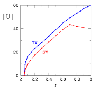
Figure 1: (Color online) Branches of traveling and standing wave states. The higher-amplitude TW branch (blue, solid) is stable near onset, while the SW branch (red, dashed) is unstable. The bifurcation to TW is degenerate, so that $||U||\sim(r-r_{H})^{1/4}$. The SW branch may undergo a secondary bifurcation at $r\approx 2.7$.

A bifurcation diagram showing the amplitudes $||U||$ where

$$||U||^{2}\equiv\int_{0}^{\lambda}dx\>dz\> \left(|\Theta(x,z,t)|^{2}\right.$$

$$+ \left.|C(x,z,t)|^{2}+|\Psi(x,z,t)|^{2}\right]$$ (17)

of the traveling waves and the standing waves is shown in figure 1. For TW, $||U||$ is independent of time and for SW, $||U||$ is evaluated at the moment at which the integral of the temperature is maximal. The abrupt onset of the TW branch reflects the fact that the Hopf bifurcation to traveling waves in thermosolutal convection with free-slip boundary conditions is degenerate Knobloch_85 ; Knobloch_89 , so that $||U||\sim(r-r_{H})^{1/4}$ rather than the usual square-root dependence. The non-monotonic behavior of the amplitude of the SW branch may indicate a secondary transition, which will not concern us in this investigation. The traveling waves are invariant under the combined Boussinesq-shift symmetry:

$$\Pi^{\rm Bouss}\Pi^{\rm Trans}_{\lambda/2} (\Theta,C,\Psi)(x,z,t)$$

$$= (-\Theta,-C,-\Psi)(x+\lambda/2,1-z,t)$$ (18)

The TW are also invariant under the family of spatio-temporal symmetries

$$\Pi^{\rm Time}_{\Delta t}\Pi^{\rm Trans}_{-v{\Delta t}} (\Theta,C,\Psi)(x,z,t)$$

$$= (\Theta,C,\Psi)(x-v{\Delta t},z,t+{\Delta t})$$ (19)

where $v\equiv\lambda/T=\omega/k$ is the velocity. Thus, the TW have $SO(2)\times Z_{2}$ symmetry. The standing waves are invariant at all times under $\ref{$}and$Π^Bouss$,i.e.theSWhave$Z_2 ×Z_2$symmetry.\par$

IV Linearization and mean fields

The usual linear stability analysis problem about the conductive state is written as

$$\partial_{t}\mathbf{u}=\mathcal{L}\mathbf{u}$$ (20)

where the infinitesimal perturbation is

$$\mathbf{u}\equiv(\tau,c,\nabla^{2}\psi)^{T}.$$ (21)

We recall that $\mathcal{L}$ encompasses the terms on the right-hand-side of (1).

A Hopf bifurcation from the conductive state takes place when the real part of an eigenvalue $\sigma_{\rm cond}\pm i\omega_{\rm cond}$ of $\mathcal{L}$ crosses zero. Because of the periodic and no-slip boundary conditions (7), eigenvectors of $\mathcal{L}$ are of the simple spatial form

$$\left(\begin{array}[]{c}\Theta_{0}\sin(kx)\sin(\pi z)\\ C_{0}\sin(kx)\sin(\pi z)\\ \Psi_{0}\cos(kx)\sin(\pi z)\end{array}\right),\left(\begin{array}[]{c}\Theta_{0}\cos(kx)\sin(\pi z)\\ C_{0}\cos(kx)\sin(\pi z)\\ \Psi_{0}\sin(kx)\sin(\pi z)\end{array}\right)$$ (28)

and linear combinations of these vectors, where $\Theta_{0}$, $C_{0}$, $\Psi_{0}$ are complex scalars. Complex eigenmodes of $\mathcal{L}$ are associated with a four-dimensional eigenspace. Some combinations of eigenmodes lead naturally to standing waves, others to traveling waves Boronska .

Our study concerns the temporal means of the traveling and standing waves. We define

$$\mathbf{\overline{U}}(x,z)\equiv\frac{1}{T}\int_{t=0}^{T}\mathbf{U}(x,z,t)dt$$ (29)

where $T$ is the temporal period. Because the temperature and concentration are important components of $\mathbf{\overline{U}}$, we refer to mean fields rather than to mean flows, contrary to the purely hydrodynamic literature. The mean field $\mathbf{\overline{U}}$ is not a solution of the governing equations. Averaging the governing equations (6), we obtain the equation obeyed by $\mathbf{\overline{U}}$, which is

$$0=\mathcal{L}\mathbf{\overline{U}}+\overline{\mathcal{N}(\mathbf{U},\mathbf{U})}=\mathcal{L}\mathbf{\overline{U}}+\mathcal{N}(\mathbf{\overline{U}},\mathbf{\overline{U}})+F$$ (30)

where

$$F\equiv\overline{\mathcal{N}(\mathbf{U}-\mathbf{\overline{U}},\mathbf{U}-\mathbf{\overline{U}})}$$ (31)

is analogous to the usual Reynolds stress force for the Navier-Stokes equations Barkley ; Gallaire and can be interpreted as the force that would have to be exerted on the system in order for the mean field to be a steady solution.

We now linearize the governing equations (6) about $\mathbf{\overline{U}}$:

$$\partial_{t}\mathbf{u}=\mathcal{L}\mathbf{u}+\mathcal{N}(\mathbf{\overline{U}},\mathbf{u})+\mathcal{N}(\mathbf{u},\mathbf{\overline{U}})\equiv\mathcal{L}_{\mathbf{\overline{U}}}\mathbf{u}$$ (32)

This procedure is not a conventional linear stability analysis since $\mathbf{\overline{U}}$ is not a steady solution unless $F=0$. For clarity, when $\mathbf{\overline{U}}$ is the mean field of nonlinear SW or TW states, the operator $\mathcal{L}_{\mathbf{\overline{U}}}$ will be denoted by $\mathcal{L}_{\rm TW}$ or $\mathcal{L}_{\rm SW}$ and its leading eigenvalues will be denoted by $\sigma^{\rm TW}_{\rm mean}\pm i\omega^{\rm TW}_{\rm mean}$ or $\sigma^{\rm SW}_{\rm mean}\pm i\omega^{\rm SW}_{\rm mean}$. These eigenmodes are the main focus of the following sections.

V Traveling waves

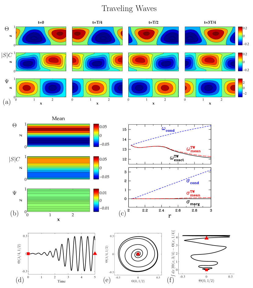
Figure 2: (Color online) (a) Instantaneous temperature, concentration and streamfunction for a traveling wave at $P=10$, $L=0.1$, $S=-0.5$ and $r=2.5$. $\Theta$ is out of phase with $C$ and $\Psi$. The Boussinesq-shift symmetry (18) is especially clear for $C$. Endpoints of ranges of $\Theta$, $C$, $\Psi$ are $\pm 0.32$, $\pm 0.46$, and $\pm 3.4$, respectively. (b) Temporally averaged fields $\overline{\Theta}$, $\overline{C}$, $\overline{\Psi}$. for this traveling wave. The functional form is approximately $\sin(2\pi z)$ and the amplitude of $\overline{\Psi}$ is much smaller than that of $\overline{\Theta}$, $\overline{C}$. Endpoints of ranges of $\Theta$, $C$, $\Psi$ are $\pm 0.065$, $\pm 0.077$ and $\pm 1.7\times 10^{-4}$, respectively. (c) Frequencies (above) and growth rates (below) as a function of Rayleigh number for traveling waves. The observed frequency ($\omega^{\rm TW}_{\rm exact}$, solid black) is closely tracked by the frequency of the traveling wave mean field ($\omega^{\rm TW}_{\rm mean}$, long-dashed red) and not at all by the frequency of the conductive state ($\omega_{\rm cond}$, short-dashed blue). The growth rate $\sigma^{\rm TW}_{\rm mean}$ is near zero, indicating that $\mathbf{\overline{U}}_{\rm TW}$ is marginally stable. The horizontal line $\sigma_{\rm marg}=0$ is used to indicate marginal stability. (d) Timeseries of $\Theta(x=\lambda/4,z=1/2)$ for $r=2.5$ from low-amplitude initial condition. Projection of conductive state is indicated by a square and of the mean field by a triangle. (e) Phase portrait showing projection of time-dependent evolution onto the temperature at $(x=0,z=1/2)$ and $(x=\lambda/4,z=1/2)$. (f) Projection onto $\Theta(x=0,z=1/2)$ and $P_{M}$ of (36), which is a proxy for projection onto the mean field.

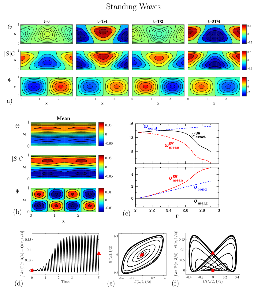
Figure 3: (Color online) (a) Instantaneous temperature, concentration and streamfunction for a standing wave at $P=10$, $L=0.1$, $S=-0.5$ and $r=2.5$. The spatial features, particularly the nodal curves, of $\Theta$ and $C$ are very similar, but there is a $T/8$ temporal shift between the two. These fields have both the Boussinesq-shift symmetry (18) and $x$-reflection symmetry (14). Endpoints of ranges of $\Theta$, $C$, $\Psi$ are $\pm 0.33$, $\pm 0.46$, and $\pm 2.6$, respectively. The color scale is the same as that of figure 2(a). (b) Temporally averaged fields $\overline{\Theta}$, $\overline{C}$, $\overline{\Psi}$ for this standing wave. Endpoints of ranges of $\Theta$, $C$, $\Psi$ are $\pm 0.043$, $\pm 0.13$, and $\pm 0.016$, respectively. The color scale is the same as that of figure 2(b). (c) Frequencies (above) and growth rates (below) as a function of Rayleigh number for standing waves. The observed frequency ($\omega^{\rm SW}_{\rm exact}$, solid black) is initially tangent to that of the conductive state ($\omega_{\rm cond}$, short-dashed blue), and then, at $r\approx 2.4$, veers downwards. The frequency of the standing wave mean field ($\omega^{\rm SW}_{\rm mean}$, long-dashed red) deviates significantly from the observed frequency almost immediately after onset, although it shows a similar downward trend. The growth rate $\sigma^{\rm SW}_{\rm mean}$ is never small and so the mean field $\mathbf{\overline{U}}_{\rm SW}$ is never marginal. (d) Timeseries of $P_{M}$ of (36) for $r=2.5$ from low-amplitude initial condition. Projection of conductive state is indicated by a square and of the mean field by a triangle. (e) Time-dependent evolution projected onto the temperature and the concentration at the same point $(x=\lambda/2,z=1/2)$. (f) Projection onto $C(x=\lambda/2,z=1/2)$ and $P_{M}$.

Figure 2(a) shows snapshots of a traveling wave $\mathbf{U}_{\rm TW}$. We show deviations $\Theta$ and $C$ from the conductive temperature and concentration profiles and the streamfunction $\Psi$ of the velocity field. Equation (10) shows that $|S|C$ is the appropriate quantity to compare with $\Theta$.

Figure 2(b) shows the mean field $\mathbf{\overline{U}}_{\rm TW}$, of this traveling wave. For traveling waves, this temporal average can be obtained by an instantaneous spatial average:

$$\mathbf{\overline{U}}_{\rm TW}(z) \equiv\frac{1}{T}\int_{0}^{T}\>dt\>\mathbf{U}_{\rm TW}(x-vt,z)$$

$$=\frac{1}{\lambda}\int_{0}^{\lambda}\>dx\>\mathbf{U}_{\rm TW}(x-vt,z)$$ (33)

and thus is necessarily independent of $x$. The mean fields are entirely different from the cellular instantaneous fields: the instantaneous fields are dominated by periodic dependence in $x$ which vanishes upon integration and a much smaller $x$-independent component.

If $\mathbf{U}$ were of the same trigonometric form as the eigenvectors (28), its spatial and temporal average would necessarily be zero. Nonlinear effects are responsible for modifying the spatial dependence of the traveling waves and creating the mean field. The form of the mean fields can be explained heuristically by the lowest order nonlinearity, namely substituting the spatial form (28) of the eigenvectors into the nonlinear term:

$$\mathcal{J}[\Psi,\Theta] =\mathcal{J}[\Psi_{0}\cos(kx)\sin(\pi z),\Theta_{0}\sin(kx)\sin(\pi z)]$$

$$=k\pi\Psi_{0}\Theta_{0}\sin(2\pi z)/2$$ (34)

and similarly for $\mathcal{J}[\Psi,C]$. Since in (28), the streamfunction is an eigenfunction of the Laplacian, the lowest order nonlinear contribution to the streamfunction equation vanishes:

$$\mathcal{J}[\Psi,\nabla^{2}\Psi]=\mathcal{J}[\Psi,-q^{2}\Psi]=0$$ (35)

Indeed, the mean fields shown in figure 2(b) have a functional form like (34) and the amplitude of the mean streamfunction is very small: $||\overline{\Psi}||/||\Psi||\sim 5\times 10^{-5}$, compared to $||\overline{\Theta}||/||\Theta||\sim||\overline{C}||/||C||\sim 0.2$, again motivating our use of the term mean field, rather than mean flow. The observations (34) and (35) are those which lead to the formulation of the three-variable Lorenz model for convection Lorenz and the five-variable Veronis model for thermosolutal convection Veronis_65 .

Figure 2(c) constitutes one of our main findings, namely that linearization about the mean field of the TWs yields an eigenvalue whose imaginary part matches the frequency of the nonlinear traveling waves and whose real part is close to zero. That is, the traveling waves in thermosolutal convection have the RZIF property, which is manifested in the figure by the fact that the long-dashed red and solid black curves coincide. The real and imaginary parts, $\sigma^{\rm TW}_{\rm mean}$ and $\omega^{\rm TW}_{\rm mean}$, of the leading eigenvalues of $\mathcal{L}_{\rm TW}$ are shown. The frequency $\omega^{\rm TW}_{\rm mean}$ agrees almost exactly with the actual frequency $\omega^{\rm TW}_{\rm exact}$ of the nonlinear traveling waves over the entire range of our study, $2<r<3$. Furthermore, the growth rate $\sigma^{\rm TW}_{\rm mean}$ of this eigenvalue remains approximately zero up to at least 50$\%$ above onset. This implies that the mean fields, viewed as solutions of the governing equations for thermosolutal convection - with the appropriate Reynolds stress forcing - are marginally stable.

Figure 2(c) also shows $\sigma_{\rm cond}$ and $\omega_{\rm cond}$, the real and imaginary parts of the leading eigenvalue of $\mathcal{L}$. Since the onset of traveling waves corresponds to a supercritical Hopf bifurcation of the conductive state, $\sigma_{\rm cond}$ crosses zero and the non-zero frequency $\omega_{\rm cond}$ necessarily agrees with the nonlinear frequency at onset. However, past the bifurcation, the frequencies diverge from one other and $\omega_{\rm cond}$ drastically overpredicts the observed value $\omega^{\rm TW}_{\rm exact}$. This is very much like the situation for the cylinder wake Barkley .

Figure 2(d)-(f) illustrates the relationship between the traveling wave $\mathbf{U}_{\rm TW}$, its mean field $\mathbf{\overline{U}}_{\rm TW}$, and the conductive state. The time series, figure 2(d), shows the temperature at a representative point. The field at $t=0$ is a small-amplitude trigonometric profile. This initial small perturbation of the conductive state grows in time and saturates as the stable traveling wave state. The frequency is initially $\omega_{\rm cond}$, but decreases as the amplitude grows, demonstrating the over-prediction of $\omega_{\rm cond}$ relative to $\omega^{\rm TW}_{\rm exact}$. The phase portraits resemble analogous ones by Barkley Barkley and by Noack Noack for the cylinder wake. Figure 2(e) plots $\Theta$ at two points on the midline separated by $\lambda/4$. The trajectory spirals out to the final saturated limit cycle. A second phase portrait in figure 2(f) has as its vertical axis

$$P_{M}\equiv\int_{0}^{\lambda}\>dx\>[\Theta(x,z=3/4)-\Theta(x,z=1/4)]$$ (36)

which approximates a projection onto the mean field. This phase portrait shows clearly that the traveling wave does not orbit around the conductive state, which is at the bottom of the figure, but instead around the mean field $\mathbf{\overline{U}}$, whose projection onto this phase plane is located at the top.

VI Standing waves

We now consider the standing waves that arises simultaneously with the traveling waves at the Hopf bifurcation and seen in figure 1. Although they are unstable, standing waves can be calculated by direct simulation by imposing reflection symmetry in $x$. Figure 3(a) shows instantaneous fields over one oscillation of a standing wave. The mean field $\mathbf{\overline{U}}_{\rm SW}$ is shown in figure 3(b). As was the case for the traveling wave, the mean field bears little resemblance to the instantaneous standing waves. However, contrary to those of the traveling wave, all of the SW mean fields vary in $x$. The primary horizontal wavenumber seen in figure 3(a) is $k$, while those seen in figure 3(b) are 0 for $\overline{\Theta}$ and $\overline{C}$ and 0 and $2k$ for $\overline{\Psi}$. Although the mean streamfunction is not as small as in the TW case, we have $||\overline{\Psi}||/||\Psi||\approx 4\times 10^{-3}$ compared to $||\overline{\Theta}||/||\Theta||\approx||\overline{C}||/||C||=0.25$.

The frequency $\omega^{\rm SW}_{\rm exact}$ of the standing waves and the leading eigenvalues of $\mathcal{L}_{\rm SW}$ are shown in figure 3(c). These behave quite differently from their traveling wave counterparts in figure 2(c). Here, $\omega^{\rm SW}_{\rm exact}$ increases with $r$ near onset and remains quite close to the frequency $\omega_{\rm cond}$ of the conductive state up to $r=2.4$, while, in contrast, the frequency $\omega^{\rm SW}_{\rm mean}$ decreases immediately after onset. However, for $r\gtrsim 2.4$, $\omega^{\rm SW}_{\rm exact}$ begins to diverge from $\omega_{\rm cond}$, veering down quite sharply starting at $r\sim 2.6$ and then less abruptly at $r\sim 2.8$, mirroring the behavior of $\omega^{\rm SW}_{\rm mean}$. The distance between $\omega^{\rm SW}_{\rm exact}$ and $\omega^{\rm SW}_{\rm mean}$ remains finite and approximately constant as the two move in tandem. In contrast $\omega_{\rm cond}$ continues to increase, thus diverging from $\omega^{\rm SW}_{\rm exact}$. Thus, although $\omega_{\rm cond}$ is a much better predictor of $\omega^{\rm SW}_{\rm exact}$ for $2.1\leq r\lesssim 2.4$, the downward trend of $\omega^{\rm SW}_{\rm exact}$ for $2.4\lesssim r\leq 3$. is tracked quite accurately by $\omega^{\rm SW}_{\rm mean}$.

In contrast to the traveling-wave case, the growth rate $\sigma^{\rm SW}_{\rm mean}$ is positive and grows linearly along with that of the conductive state; $\mathbf{U}_{\overline{{\rm SW}}}$ is not a marginally stable state. For $r\gtrsim 2.4$, $\sigma_{\rm cond}$ continues to increase linearly, while $\omega^{\rm SW}_{\rm mean}$ increases more steeply for $2.6\lesssim r\lesssim 2.8$ and then tapers off for $2.8\lesssim r\lesssim 3$. Thus, the approach of $\omega^{\rm SW}_{\rm mean}$ towards $\omega^{\rm SW}_{\rm exact}$ for $r\gtrsim 2.4$ is not matched by an approach of $\sigma^{\rm SW}_{\rm mean}$ towards zero. In summary, the standing waves in thermosolutal convection do not have the RZIF property, as manifested in the figure by the fact that the long-dashed red and solid black lines are far from one another. The real part of the mean-field eigenvalue is far from zero and the frequency does not match the observed nonlinear frequency.

Figure 3(d)-(f) illustrates the dynamics of the approach to the standing wave, via a timeseries and two phase portraits. Figure 3(d), a timeseries of the mean-field projection proxy (36), shows a brief oscillation about the conductive state followed by saturated oscillations about the mean field. The phase portrait in Fig. 3(e) shows the instantaneous temperature and concentration at the domain midpoint; in this projection, the standing wave traces out a trapezoid, oriented along the positive diagonal, corresponding to the $T/8$ temporal phase shift between the two fields. The phase portrait in Fig. 3(f) demonstrates the difference between the standing and traveling wave dynamics: the projection onto the mean field is far from constant. An important second harmonic component is visible in Fig. 3(f), since a maximum in (36) corresponds alternately to a minimum and a maximum in $C(\lambda/2,1/2)$.

VII Temporal spectra

We now present a simple but general analysis giving conditions under which the RZIF property is guaranteed. Consider any evolution equation

$$\partial_{t}\mathbf{U} =\mathcal{L}\mathbf{U}+\mathcal{N}(\mathbf{U},\mathbf{U})$$ (37)

where $\mathcal{L}$ is linear and $\mathcal{N}(\cdot,\cdot)$ is a quadratic nonlinearity. Let

$$\mathbf{U}=\mathbf{\overline{U}}+\sum_{n\neq 0}\mathbf{u}_{n}e^{in\omega t}$$ (38)

(with $\mathbf{u}_{-n}=\mathbf{u}_{n}^{\ast}$) be the temporal Fourier decomposition of a periodic solution to (37) with mean $\mathbf{\overline{U}}$ and frequency $\omega$. Substituting (38) into (37) leads to

$$\sum_{n\neq 0}in\omega\mathbf{u}_{n}e^{in\omega t}=\mathcal{L}\mathbf{\overline{U}}+\mathcal{N}(\mathbf{\overline{U}},\mathbf{\overline{U}})+\sum_{m\neq 0}\mathcal{N}(\mathbf{u}_{m},\mathbf{u}_{-m})$$

$$+\sum_{n\neq 0}\mathcal{L}\mathbf{u}_{n}e^{in\omega t}+\sum_{n\neq 0}\left(\mathcal{N}(\mathbf{\overline{U}},\mathbf{u}_{n})+\mathcal{N}(\mathbf{u}_{n},\mathbf{\overline{U}})\right)e^{in\omega t}$$

$$+\sum_{n\neq 0}\sum_{m\neq 0,n}\mathcal{N}(\mathbf{u}_{m},\mathbf{u}_{n-m})e^{in\omega t}$$ (39)

Separating (39) by frequency leads to an equation for the zero frequency terms:

$$0 =\mathcal{L}\mathbf{\overline{U}}+\mathcal{N}(\mathbf{\overline{U}},\mathbf{\overline{U}})+\sum_{m\neq 0}\mathcal{N}(\mathbf{u}_{m},\mathbf{u}_{-m})$$ (40)

which is the same as Eq. (30) satisfied by the mean field, and equations for the nonzero frequency terms ($n\geq 1$):

$$in\omega\mathbf{u}_{n} =\mathcal{L}\mathbf{u}_{n}+\mathcal{N}(\mathbf{\overline{U}},\mathbf{u}_{n})+\mathcal{N}(\mathbf{u}_{n},\mathbf{\overline{U}})$$

$$+\sum_{m\neq 0,n}\mathcal{N}(\mathbf{u}_{m},\mathbf{u}_{n-m})$$ (41)

The first three terms on the right-hand-side of this expression are just those defining the linearization about $\mathbf{\overline{U}}$. Hence, for $n\geq 1$ we have

$$in\omega\mathbf{u}_{n} =\mathcal{L}_{\mathbf{\overline{U}}}\mathbf{u}_{n}+\mathcal{N}_{n}$$ (42)

where $\mathcal{N}_{n}\equiv\sum_{m\neq 0,n}\mathcal{N}(\mathbf{u}_{m},\mathbf{u}_{n-m})$. For example:

$$\mathcal{N}_{1} =\mathcal{N}(\mathbf{u}_{2},\mathbf{u}_{-1})+\mathcal{N}(\mathbf{u}_{-1},\mathbf{u}_{2})$$

$$\qquad+\mathcal{N}(\mathbf{u}_{3},\mathbf{u}_{-2})+\mathcal{N}(\mathbf{u}_{-2},\mathbf{u}_{3})+\ldots$$ (43a)

$$\mathcal{N}_{2} =\mathcal{N}(\mathbf{u}_{1},\mathbf{u}_{1})+\mathcal{N}(\mathbf{u}_{3},\mathbf{u}_{-1})+\mathcal{N}(\mathbf{u}_{-1},\mathbf{u}_{3})$$

$$\qquad+\mathcal{N}(\mathbf{u}_{4},\mathbf{u}_{-2})+\mathcal{N}(\mathbf{u}_{-2},\mathbf{u}_{4})+\ldots$$ (43b)

$$\mathcal{N}_{3} =\mathcal{N}(\mathbf{u}_{1},\mathbf{u}_{2})+\mathcal{N}(\mathbf{u}_{2},\mathbf{u}_{1})$$

$$\qquad+\mathcal{N}(\mathbf{u}_{4},\mathbf{u}_{-1})+\mathcal{N}(\mathbf{u}_{-1},\mathbf{u}_{4})+\ldots$$ (43c)

If $\mathbf{u}_{2}=\mathbf{u}_{3}=\ldots=0$, i.e. if the periodic cycle is exactly monochromatic, then $\mathcal{N}_{1}=0$ and

$$i\omega\mathbf{u}_{1}=\mathcal{L}_{\mathbf{\overline{U}}}\mathbf{u}_{1}$$ (44)

i.e. $\mathcal{L}_{\mathbf{\overline{U}}}$ has an eigenvalue whose real part is zero and whose imaginary part is the frequency of the periodic solution. Hence the RZIF property necessarily follows for monochromatic oscillations in a system with quadratic nonlinearity.

More generally if, as is often the case,

$$||u_{n}||\sim\epsilon^{|n|}$$ (45)

then

$$\underbrace{i\omega\mathbf{u}_{1}}_{\epsilon}-\underbrace{\mathcal{L}_{\mathbf{\overline{U}}}\mathbf{u}_{1}}_{\epsilon}=\underbrace{\mathcal{N}_{1}}_{\epsilon^{3}}$$ (46)

so that (44) holds approximately.

The validity of (44) or (46) does not require that $\mathcal{N}_{n}$ be negligible in (42) for higher harmonics $n>1$ and indeed it is not. Assuming the scaling (45), equations (43) show that for $n\geq 2$, $\mathcal{N}_{n}$ is of the same order as the other terms in (42), e.g.

$$\underbrace{i2\omega\mathbf{u}_{2}-\mathcal{L}_{\mathbf{\overline{U}}}\mathbf{u}_{2}}_{\epsilon^{2}}=\underbrace{\mathcal{N}_{2}}_{\epsilon^{2}},\qquad\underbrace{i3\omega\mathbf{u}_{3}-\mathcal{L}_{\mathbf{\overline{U}}}\mathbf{u}_{3}}_{\epsilon^{3}}=\underbrace{\mathcal{N}_{3}}_{\epsilon^{3}}$$ (47)

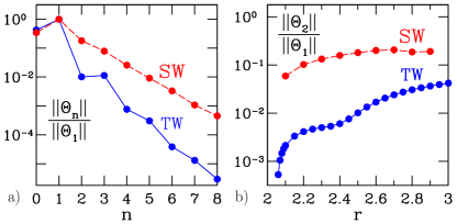
Figure 4: (Color online) Temporal spectra of temperature field of traveling and standing waves. (a) Full temporal spectrum for $r=2.5$, i.e. $||\Theta_{n}||$ for multiples $n$ of the observed frequency. (b) Ratio $||\Theta_{2}||/||\Theta_{1}||$ as a function of $r$. The spectrum of the traveling waves (blue, solid) is far more peaked at $n=1$ than that of the standing waves (red, dashed).

Although (44) is linear in $\mathbf{u}_{1}$, the mean flow equation (40) is quadratic in $\mathbf{u}_{1}$, insuring the saturation of its amplitude, as shown more explicitly in system (48) below. Quadratic interaction of $\mathbf{u}_{1}$ with itself takes two forms: $\mathcal{N}(\mathbf{u}_{1},\mathbf{u}_{-1})+\mathcal{N}(\mathbf{u}_{-1},\mathbf{u}_{1})$ leads the mean flow $\mathbf{\overline{U}}$ to differ from the base flow, while $\mathcal{N}(\mathbf{u}_{1},\mathbf{u}_{1})$ generates $\mathbf{u}_{2}$. RZIF is favored by small $\mathbf{u}_{2}$, and hence by small $\mathcal{N}(\mathbf{u}_{1},\mathbf{u}_{1})$. On the other hand, since RZIF requires a mean field which differs from the base field, $\mathcal{N}(\mathbf{u}_{1},\mathbf{u}_{-1})+\mathcal{N}(\mathbf{u}_{-1},\mathbf{u}_{1})$ should be non-negligible. Nonlinear saturation of amplitudes of instabilities in a more usual non-RZIF context is addressed in texts such as Manneville Manneville and Iooss and Joseph Iooss_Joseph .

The reasoning above does not provide an a priori reason for which an eigenvalue of the mean field would predict the frequency, since no method has been given for determining whether the oscillatory state is almost monochromatic. It does, however, connect these two properties. The frequency of a monochromatic or almost-monochromatic oscillation in a system with quadratic nonlinearity should be well predicted by the leading eigenvalue of $\mathcal{L}_{\mathbf{\overline{U}}}$.

Returning to the thermosolutal system, figure 4 contrasts the temporal spectra of the temperature field of the traveling and standing waves. Figure 4(a). shows that the spectrum of the traveling wave at $r=2.5$ is concentrated at $n=1$, i.e. at the observed frequency. The spectrum of the standing waves is far wider, with substantial amplitude for $n\geq 2$. The ratio $||\Theta_{2}||/||\Theta_{1}||$ is $10^{-2}$ for TW and 20 times higher than this for SW.

Figure 4(b) shows that this trend holds over our range $2\leq r\leq 3$ of observation, by plotting $||\Theta_{2}||/||\Theta_{1}||$ as a function of $r$. Interestingly, for TW this ratio shows an upturn at $r\approx 2.5$, which is where figure 2(c) shows that $\sigma^{\rm TW}_{\rm mean}+i\omega^{\rm TW}_{\rm mean}$ begins to deviate from $0+i\omega^{\rm TW}_{\rm exact}$. For SW, there seems to be little or no correlation between the $r$-dependence of the temporal spectrum and that of $\sigma^{\rm SW}_{\rm mean}+i\omega^{\rm SW}_{\rm mean}$, which is to be expected if the relationship between the two requires a peaked spectrum.

The RZIF property is corroborated by order-of-magnitude comparison of the terms in equations (46). Examining the equations corresponding to the temperature field for TW at $r=2.5$, the ratio of the maximum of the right-hand-side (which we wish to neglect) to that of the left-hand-side is 0.025. Comparing the quadratic terms which appear in the temperature equation, we find that the ratio between $\mathcal{J}[\Psi_{1},\Theta_{1}]$ and $\mathcal{J}[\Psi_{1},\Theta_{-1}]+\mathcal{J}[\Psi_{-1},\Theta_{1}]$ is 0.1.

The spectra of the other fields comprising ${\bf U}$ also follow this tendency, but not to the dramatic extent of $\Theta$. The concentration field at $r=2.5$ has $||C_{2}||/||C_{1}||\approx 0.1$ for TW (ten times larger than for $\Theta$) and 0.2 for SW (the same as for $\Theta$). Similarly, for the TW concentration field, the ratio of the maximum of the right-hand-side of (46) to that of the left-hand-side is 0.2 (ten times this ratio for $\Theta$). The ratio between the quadratic terms which appear in the concentration equation, $\mathcal{J}[\Psi_{1},C_{1}]$ and $\mathcal{J}[\Psi_{1},C_{-1}]+\mathcal{J}[\Psi_{-1},C_{1}]$, is 0.4.

VIII Relation to previous work on cylinder wake

In light of these results, we review some of the previous work concerning RZIF. Linear stability analysis of the mean field has been carried out only for open flows and almost exclusively for the cylinder wake. Hammond and Redekopp Redekopp , Pier Pier , Barkley Barkley and Mittal Mittal have shown that the frequency of the cylinder wake is predicted with remarkable accuracy by that of the mean field even quite far above onset, at least until $Re=180\approx 4Re_{\rm H}$. In keeping with our conjecture that RZIF coincides with a monochromatic oscillation, Dusek et al. Dusek have found experimentally that the temporal spectrum is highly peaked even at high Reynolds numbers. Knobloch et al. Knobloch_89 find that the traveling waves in a minimal model of thermosolutal convection are almost monochromatic, while the standing waves at the same parameter values are not.

Sipp and Lebedev Sipp carried out a numerical weakly nonlinear analysis of the cylinder wake about the Hopf bifurcation point, and were able to reproduce the slope of the frequency as well as the zero growth rate. More specifically, they approximated the flow $\mathbf{U}$ and its frequency $\omega$, its mean flow $\mathbf{\overline{U}}$ and the eigenvalues of this mean flow $\sigma_{\mathbf{\overline{U}}}\pm i\omega_{\mathbf{\overline{U}}}$ near onset $Re_{\rm H}$ and found agreement between the slopes of the mean field frequency and the nonlinear frequency $\omega_{\mathbf{\overline{U}}}^{\prime}(Re_{H})\approx\omega^{\prime}(Re_{H})$ as well as marginal stability $\sigma_{\mathbf{\overline{U}}}\approx 0$. They did not capture its further evolution with $Re$, for example its curvature at $Re_{\rm H}$, which would have required extending the analysis to higher order.

More fundamentally, Sipp and Lebedev Sipp determined which of the contributions to the lowest-order nonlinear term were required to be small in order to achieve this agreement. These terms arise from the second temporal harmonic, just as we have found. They also presented an important counter-example. Performing the same weakly nonlinear analysis on the flow in an open driven cavity, they found both that the second harmonic contributions to the nonlinear term were not small and also that the weakly nonlinear analysis did not reproduce $\omega^{\prime}(Re_{H})$. This counter-example shows that RZIF does not hold for all flows and also corroborates the role of the second temporal harmonic.

Our attempt to carry out a weakly nonlinear analysis analogous to that of Sipp and Lebedev Sipp was hampered by the degeneracy of the Hopf bifurcation to traveling waves in thermosolutal convection with free-slip boundary conditions Knobloch_85 ; see figure 1. The cubic term in the normal form is zero, requiring the calculation of a quintic term or an appropriate model Knobloch_89 . The bifurcation to standing waves is free from this pathology, but, as shown in section VI, the mean fields of the standing waves do not have the desired property near onset.

Mantič-Lugo et al. Gallaire proposed the following system

$$0 =\mathcal{L}\mathbf{\overline{U}}+\mathcal{N}(\mathbf{\overline{U}},\mathbf{\overline{U}})+A^{2}\mathcal{N}(\mathbf{u}_{1},\mathbf{u}_{-1})$$ (48a)

$$(\sigma+i\omega)\mathbf{u}_{1} =\mathcal{L}_{\mathbf{\overline{U}}}\mathbf{u}_{1}\qquad\qquad||u_{1}||=1$$ (48b)

$$\sigma =0$$ (48c)

as a means of calculating $\mathbf{\overline{U}}$ and $\omega$ for the cylinder wake without recourse to time integration. Equation (48a) is a truncated version of the exact equation (40) satisfied by the mean field; consequently, its validity requires a stongly peaked spectrum, as emphasized by Mantič-Lugo et al. Gallaire . Starting from an estimate of the mean field by the base flow, their equivalent of the conductive state, they solved (48b) for the eigenvalue $(\sigma+i\omega)$ and the eigenvector $\mathbf{u}_{1}$. Substituting $\mathbf{u}_{1}$ in (48a), they computed a new mean field $\mathbf{\overline{U}}$. The amplitude $A$ multiplying the eigenvector was adjusted until convergence to marginal stability $\sigma=0$. Our attempt to carry out this iterative procedure for the thermosolutal system did not converge.

IX Conclusion

A number of fluid-dynamical researchers have attempted to relate the nonlinear frequency of a periodic state, primarily the cylinder wake, with the imaginary part of the eigenvalue of the evolution operator linearized about the temporal mean. Following this line of investigation, we have studied the traveling waves and standing waves resulting from the Hopf bifurcation in thermosolutal convection. The traveling waves have turned out to be a textbook case of RZIF, i.e. the real part of the mean-flow eigenvalue is almost exactly zero and the imaginary part is almost exactly the frequency. In contrast the standing waves do not have this property: the mean-flow eigenvalue performs even worse than the base-flow eigenvalue at predicting the frequency. These results are displayed in our summary diagram, figure 5.

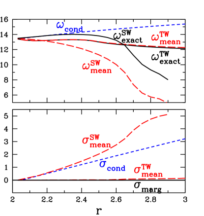
Figure 5: (Color online) Frequencies (above) and growth rates (below) for TW and SW. The mean eigenvalues (long-dashed red) track the exact frequency and marginal growth rate (solid black) very closely for TW and not at all for SW.

Guided by these results, we have put forth a general theoretical explanation for the RZIF property in terms of the temporal spectrum. If the periodic oscillation is monochromatic, then RZIF is satisfied exactly. If it is not exactly monochromatic but the higher temporal harmonics are small, then RZIF should be satisfied approximately. This corresponds to the traveling/standing wave dichotomy: the spectrum of the traveling waves is sharply peaked, while that of the standing waves is not. The question which remains is that of predicting the width of the spectrum of periodic states.

Appendix A Numerical Methods

Because of the horizontally periodic and vertical no-slip boundary conditions (7), the fields can be represented as

$$\mathbf{U}(x,z,t)=\sum_{n}\hat{\mathbf{U}}_{mn}(t)e^{imkx}\sin(n\pi z)$$ (49)

for which spatial derivatives are easily taken. A two-dimensional Fourier transform leads to values on an equally spaced grid, where the multiplications in the Poisson bracket $\mathcal{J}$ of (2) are performed.

In order to solve

$$\partial_{t}\mathbf{U} =\mathcal{L}\mathbf{U}(t)+\mathcal{N}(\mathbf{U},\mathbf{U})$$ (50)

we use first-order explicit-implicit time discretization, i.e. backwards Euler for the diffusive terms and forwards Euler for all other terms.

$$\mathbf{U}(t+{\Delta t}) =(I-{\Delta t}\mathcal{L})^{-1}(I+{\Delta t}\mathcal{N})\mathbf{U}(t)$$ (51)

$$\equiv B\mathbf{U}(t)$$

In order to explain the method by which traveling waves are calculated, we begin by discussing the calculation of steady states. We adapt the timestepping scheme (51) to carry out Newton’s method as follows Mamun :

$$\mathbf{U}(t+{\Delta t})-\mathbf{U}(t)= \left[\left(I-{\Delta t}\mathcal{L}\right)^{-1}\left(I+{\Delta t}\mathcal{N}\right)-I\right]\mathbf{U}(t)$$

$$=\left(I-{\Delta t}\mathcal{L}\right)^{-1} \left[I+{\Delta t}\mathcal{N}-\left(I-{\Delta t}\mathcal{L}\right)\right]\mathbf{U}(t)$$

$$=\left(I-{\Delta t}\mathcal{L}\right)^{-1} {\Delta t}\left(\mathcal{N}+\mathcal{L}\right)\mathbf{U}(t)$$ (52)

Thus, the roots of $\mathcal{N}+\mathcal{L}$ are the same as those of $B-I$, where $B$ is the timestepping operator (51). The calculation (52) holds for any value of ${\Delta t}$ regardless of size, in contrast to (51), whose validity as a timestepping scheme relies on a Taylor series approximation in ${\Delta t}$ and so requires ${\Delta t}$ small. One Newton step is then formulated as

$$(B_{\mathbf{U}}-I)\mathbf{u} =(B-I)(\mathbf{U})$$ (53)

$$\mathbf{U} \leftarrow\mathbf{U}-\mathbf{u}$$

where

$$B_{\mathbf{U}}\mathbf{u} \equiv(I-{\Delta t}\mathcal{L})^{-1}(\mathbf{u}+{\Delta t}(\mathcal{N}(\mathbf{U},\mathbf{u})+\mathcal{N}(\mathbf{u},\mathbf{U}))$$ (54)

is the linearization of $B$ about the current solution estimate $\mathbf{U}$ and $\mathbf{u}$ is the decrement to be calculated and applied to $\mathbf{U}$. For large ${\Delta t}$, the linear operator $B_{\mathbf{U}}-I$ is well conditioned, unlike the usual Jacobian operator $\mathcal{N}_{\mathbf{U}}+\mathcal{L}$. BICGSTAB Vandervorst is used to solve the linear equation (53) for $\mathbf{u}$, thus avoiding the storage and even the construction of the Jacobian operator.

In the horizontally periodic domain, solutions are not unique but defined only up to a spatial phase; equivalently, the Jacobian is singular, with the marginal $x$-translation of $\mathbf{U}$ as a null vector. (Although the image of the Jacobian $B_{\mathbf{U}}-I$ is not of full rank, a vector produced by action of $B-I$ is always in its image.) A singular linear system can, however, be solved by iterative conjugate gradient methods without imposing any additional phase condition, since the solution is constructed from a set of vectors created by repeated action of the linear operator on an initial vector, which is unaffected by the singularity of the Jacobian. The solution $\mathbf{u}$ returned by BICGSTAB will be one of the possible solutions of (53), whose phase is determined by that of the right-hand-side $\mathbf{U}$.

Traveling wave solutions are of the form

$$\mathbf{U}(x,z,t) =\mathbf{U}(x-Vt,z)$$ (55)

where $V$ is the unknown velocity. Substituting (55) into the governing equation (50) leads to

$$0 =\mathcal{L}\mathbf{U}+\mathcal{N}(\mathbf{U},\mathbf{U})+V\partial_{x}\mathbf{U}$$ (56)

so that $(\mathbf{U},V)$ together describe a steady state. We redefine $B$ and its linearization as:

$$B(\mathbf{U},V)=(I-{\Delta t}\mathcal{L})^{-1}[\mathbf{U}+{\Delta t}(\mathcal{N}(\mathbf{U},\mathbf{U})+V\partial_{x}\mathbf{U})]$$ (57)

$$B_{\mathbf{U},V}(\mathbf{u},v)=(I-{\Delta t}\mathcal{L})^{-1}$$

$$\qquad[\mathbf{u}+{\Delta t}(\mathcal{N}(\mathbf{U},\mathbf{u})+\mathcal{N}(\mathbf{u},\mathbf{U})+V\partial_{x}\mathbf{u}-v\partial_{x}\mathbf{U})]$$ (58)

For any periodic orbit the solution is defined only up to a temporal phase. Unlike in the case of a spatial phase, here it is necessary to impose an additional equation since $V$ is an additional unknown. The easiest option is to fix the zero-crossing of one of the elements of $\mathbf{U}$ by specifying that it remain unchanged by the Newton step. (Since the fields we compute are deviations from the linear profile, all of them cross zero at any height $z$; any such zero-crossing can be set as a condition, i.e. $u_{p}=0$.) Since $u_{p}$ is to be set to zero, a computational simplification can be realized by storing $v$ in this element. The subroutine corresponding to the action of $B_{\mathbf{U},V}$ begins by extracting $v$ from $u_{p}$, replacing $u_{p}$ by its imposed value of zero:

$$\begin{array}[]{cl}v&\leftarrow u_{p}\\ u_{p}&\leftarrow 0\end{array}$$ (61)

and then acting with $B_{\mathbf{U},V}$. This procedure is repeated when a solution is returned by BICGSTAB before decrementing:

$$\begin{array}[]{cl}\mathbf{U}&\leftarrow\mathbf{U}-\mathbf{u}\\ V&\leftarrow V-v\end{array}$$ (64)

Standing waves, which cannot be calculated in this way, are computed by integrating in time while imposing reflection symmetry in $x$.

We calculate leading eigenvalues by constructing and then diagonalizing the Jacobian, restricting computation to the horizontal wavenumber $k$.

References

- (1) C.H.K. Williamson, Defining a universal and continuous Strouhal-Reynolds number relationship for the laminar vortex shedding of a circular cylinder Phys. Fluids 31, 2742 (1988).
- (2) J. Dušek, P. Le Gal, and P. Fraunié, A numerical and theoretical study of the first Hopf bifurcation in a cylinder wake, J. Fluid Mech. 264, 59 (1994).
- (3) C.P. Jackson, A finite-element study of the onset of vortex shedding in flow past variously shaped bodies, J. Fluid Mech. 182, 23 (1987).
- (4) D.A. Hammond and L.G. Redekopp, Global dynamics of symmetric and asymmetric wakes, J. Fluid Mech. 331, 231 (1997).
- (5) B. Pier, On the frequency selection of finite-amplitude vortex shedding in the cylinder wake, J. Fluid Mech. 458, 407 (2002).
- (6) D. Barkley, Linear analysis of the cylinder wake mean flow, Europhys. Lett. 75, 750 (2006).
- (7) S. Mittal, Global linear stability analysis of time-averaged flows, Int. J. Numer. Meth. Fluids 58, 111 (2007).
- (8) W. V. R. Malkus, Outline of a theory of turbulent shear flow, J. Fluid Mech. 1, 521 (1956).
- (9) J. T. Stuart, On the non-linear mechanics of hydrodynamic stability, J. Fluid Mech. 4, 1 (1958).
- (10) B.J.A. Zielinska, J.E. Wesfreid, On the spatial structure of global modes in wake flow, Phys. Fluids 7, 1418 (1995).
- (11) A. Maurel, V. Pagneux, J.E. Wesfreid, Mean-Flow Correction as Non-Linear Saturation Mechanism, Europhys. Lett. 32, 217 (1995).
- (12) B. R. Noack, K. Afanasiev, M. Morzynski, G. Tadmor, and F. Thiele, A hierarchy of low-dimensional models for the transient and post-transient cylinder wake, J. Fluid Mech. 497, 335 (2003).
- (13) D. Sipp and A. Lebedev, Global stability of base and mean flows: a general approach and its applications to cylinder and open cavity flows, J. Fluid Mech. 593, 333 (2007).
- (14) V. Mantič-Lugo, C. Arratia, F. Gallaire, Self-consistent mean flow description of the nonlinear saturation of the vortex shedding in the cylinder wake, Phys. Rev. Lett. 113, 084501 (2014).
- (15) Lord Rayleigh, On convection currents in a horizontal layer of fluid, when the higher temperature is on the under side, Philos. Mag. 32 529 (1916).
- (16) L.S. Tuckerman, Thermosolutal and binary fluid convection as a matrix problem, Physica D 156, 325 (2001).
- (17) E. Knobloch, Oscillatory convection in binary mixtures, Phys. Rev. A 34, 1538 (1986).
- (18) E. Knobloch, Double Diffusive Motions, in Proc. 1985 Joint ASCE-ASME Mechanics Conference, ed. N.E. Bixler & E.A. Spiegel (Fluid Eng. Div., ASME, New York), Vol. 24, p. 17, 1985.
- (19) E. Knobloch, A. E. Deane, J. Toomre, A model of double-diffusive convection with periodic boundary conditions, Contemp. Math. 99, 339 (1989).
- (20) K. Boronska & L.S. Tuckerman, Standing and travelling waves in cylindrical Rayleigh-Benard convection, J. Fluid Mech. 559, 279 (2006).
- (21) E.N. Lorenz, Deterministic nonperiodic flow J. Atm. Sci. 20, 130 (1963).
- (22) G. Veronis, On finite-amplitude instability in thermohaline convection, J. Mar. Res. 23, 1 (1965).
- (23) P. Manneville, Dissipative Structures and Weak Turbulence, Academic Press, San Diego, 1990.
- (24) G. Iooss & D.D. Joseph, Elementary Stability and Bifurcation Theory, Springer-Verlag, New York, 1980.
- (25) C.K. Mamun & L.S. Tuckerman, Asymmetry and Hopf bifurcation in spherical Couette flow, Phys. Fluids 7, 80 (1995).
- (26) H.A. van der Vorst, Bi-CGSTAB: A fast and smoothly converging variant of Bi-CG for the solution of nonsymmetric linear systems, SIAM J. Sci. Stat. Comput. 13, 631 (1992).