Nonlinear generalized source method for modeling second-harmonic generation in diffraction gratings

Abstract

We introduce a versatile numerical method for modeling light diffraction in periodically patterned photonic structures containing quadratically nonlinear non-centrosymmetric optical materials. Our approach extends the generalized source method to nonlinear optical interactions by incorporating the contribution of nonlinear polarization sources to the diffracted field in the algorithm. We derive the mathematical formalism underlying the numerical method and introduce the Fourier-factorization suitable for nonlinear calculations. The numerical efficiency and runtime characteristics of the method are investigated in a set of benchmark calculations: the results corresponding to the fundamental frequency are compared to those obtained from a reference method and the beneficial effects of the modified Fourier-factorization rule on the accuracy of the nonlinear computations is demonstrated. In order to illustrate the capabilities of our method, we employ it to demonstrate strong enhancement of second-harmonic generated in one- and two-dimensional optical gratings resonantly coupled to a slab waveguide. Our method can be easily extended to other types of nonlinear optical interactions by simply incorporating the corresponding nonlinear polarization sources in the algorithm.

I Introduction

Higher-harmonic generation is a fundamental nonlinear optical process that has attracted intense interest ever since the beginnings of nonlinear optics bp62pr ; p63pr . Generation of optical waves via nonlinear interaction provides an effective approach to explore the properties of light matter interaction at fundamental level and, equally important, has found key applications in many areas of science and technology. While most of the early studies of higher-harmonic generation focused on wave interaction in homogeneous nonlinear optical media, recent advances in nanofabrication techniques and the advent of metamaterials have considerably broadened the experimental and theoretical framework in which these nonlinear optical processes are explored. In particular, second-harmonic generation (SHG) from isotropic fzp06nl ; kew06s ; nsh06prl and chiral vsv10prl ; vbc14am metasurfaces, layered media coupled to arrays of plasmonic particles cdh07nl , and quantum engineered plasmonic metasurfaces lta14n has been observed.

A key prerequisite condition for achieving efficient SHG is that the wavevectors of the interacting waves are phase-matched. One particularly efficient method to phase match optical waves is by using diffraction gratings. In this approach, the residual wavevector imbalance is canceled by the grating wavevector, $\kappa=2\pi/\Lambda$, where $\Lambda$ is the grating period. Importantly, the wide range of geometrical and materials parameters characterizing a diffraction grating allows one to employ such optical devices to achieve wavevector phase matching in a multitude of optical wave configurations. More importantly in this context, strong optical field enhancement and, consequently, a significantly more efficient nonlinear optical interaction can be achieved by using metallic gratings. Because generally there is no explicit analytical solution to the problem of diffraction by periodic structures, efficient and accurate numerical methods are essential for the design of diffraction gratings with predefined spectral characteristics. Solving this problem in the nonlinear case is an even more daunting task, chiefly because the larger number of interacting waves and their intricate interplay significantly increases the complexity of the problem.

The periodic nature of diffraction gratings renders frequency (wavevector) domain methods based on the Floquet-Bloch theorem to be particularly suitable algorithms for describing such optical structures. A common characteristic of these methods is the Fourier expansion of the optical field in a suitably chosen basis of modes, the main unknowns to be found being the corresponding Fourier coefficients. Among the most used methods in this class one should mention the Fourier modal method (FMM), also known as rigorous coupled-wave analysis (RCWA) mgp95josaa ; l97josaa ; lm96josaa ; srk07josaa ; eb10oe , the C-method crm80jo ; lcg99ao for corrugated gratings, and Green’s function type of methods s87josab ; ms05josaa ; st12jqsrt . On the other hand, there is a scarcity of numerical methods for SHG and other nonlinear interactions in periodic structures and the convergence and runtime behavior of the few that do exist are not as well characterized. These methods are either problem specific algorithms pn94josab or extensions of linear methods to the nonlinear case, e.g. the FMM ntf02josaa ; btf07josab ; prl10josab , finite-difference time-domain method lh04josab ; rmj06jlt , Green’s function method cy02prb , and multiple scattering matrix method bp10prb ; xz12oe .

In this work we show how the linear generalized source method (GSM) st12jqsrt ; st10jqe can be adapted to describe the SHG in diffraction gratings containing non-centrosymmetric materials. We choose the linear GSM as a starting platform for our new method because it has proven to be an efficient alternative to the FMM for the analysis of one- and two-dimensional (1D, 2D), corrugated, periodic optical structures. Its optimal runtime is of order $N_{o}\log(N_{o})$, where $N_{o}$ is the total number of diffraction orders, as compared to $N_{o}^{3}$ for the conventional FMM. The key ingredients needed to achieve this remarkable computational efficiency is the use of a matrix-multiplication based iterative solver, namely the generalized minimum residual (GMRES) method, to solve an underlying linear system of coupled integral equations and a fast Toeplitz-matrix-vector multiplication performed by means of a fast-Fourier transform (FFT). In addition, its implicit, Green’s function type formulation of Maxwell equations allows for a natural incorporation of nonlinear source terms, which is the main challenge in computing the SHG response.

The rest of the paper is organized as follows: in Section II we introduce the formulation of the nonlinear GSM, including the correct Fourier-factorization rule, and present the proper discretization of the underlying equations that allows one to use a fast iterative solver. Then, in Section III, the convergence and runtime behavior of the method are studied. The method is applied to optimize the radiated second-harmonic (SH) by a diffraction grating coupled to a slab waveguide in Section IV before final conclusions are drawn in Section V.

II Derivation of the nonlinear generalized source method

We start the derivation of the nonlinear GSM from the governing equations for SHG in the frequency domain and describe the general solution strategy. We then derive the nonlinear GSM for 2D periodic structures following st12jqsrt and extend its scope to the SHG in optical gratings containing non-controsymmetric materials.

II.1 Physical model for second-harmonic generation

We consider a quadratically nonlinear optical medium and a time-harmonic electric field, $\bm{\mathcal{E}}({\bf x},t)$, propagating in the medium at the fundamental frequency (FF), $\omega_{0}$,

$$\bm{\mathcal{E}}({\bf x},t)={\bf E}({\bf x})e^{i\omega_{0}t}+c.c.,$$ (1)

where ${\bf x}$ and $t$ are the position vector and time, respectively. Through nonlinear interaction with the optical medium, this field gives rise to a nonlinear source polarization, $\bm{\mathcal{P}}({\bf x},t)={{\bf P}^{\text{NL}}}({\bf x})\exp(i\Omega t)+c.c.$, which oscillates at the SH frequency, $\Omega=2\omega_{0}$. This polarization is the source of the electromagnetic field generated at the SH and is related to the excitation field via a third-order nonlinear susceptibility tensor, ${{\bm{\chi}}^{(2)}}$:

$$P_{\gamma}^{\mathrm{NL}}({\bf x})=\sum_{\alpha,\beta}\chi^{(2)}_{\gamma\alpha\beta}E_{\alpha}({\bf x})E_{\beta}({\bf x}).$$ (2)

In this equation and what follows, Greek indices take the values of the Cartesian coordinates $x$, $y$, and $z$.

Under the undepleted pump approximation, the initially nonlinear problem in the time-domain is solved in three steps: i) Calculate the field at the FF, $\omega_{0}$; ii) evaluate the nonlinear polarization generated at the SH via Eq. (2); and iii) calculate the field at the SH. The first and last steps are performed using the linear and nonlinear (extended) versions of the GSM, respectively.

II.2 The GSM for inhomogeneous problems

At both the FF and SH, the electromagnetic field is governed by the electromagnetic wave equation with a physical source current, ${\bf J}^{\text{ext}}({\bf x})$,

$$\nabla\times\nabla\times{\bf E}-\omega^{2}\mu_{0}\varepsilon{\bf E}=i\omega\mu_{0}{\bf J}^{\text{ext}},$$ (3)

where for convenience we have suppressed the spatial dependence of the variables and we introduced a generic frequency, $\omega$, that takes the values $\omega=\omega_{0}$ ($\omega=\Omega$) at the FF (SH). In Eq. (3), $\varepsilon({\bf x})$ is the spatial distribution of the electric permittivity that defines the grating.

The GSM is a rigorous method for solving Eq. (3). It is based on the decomposition of $\varepsilon({\bf x})$ defining the grating into a simple background structure with permittivity, $\varepsilon_{b}({\bf x})$, and the difference structure, $\Delta\varepsilon({\bf x})=\varepsilon({\bf x})-\varepsilon_{b}({\bf x})$. The background has to be chosen such that the linear solution operator ${{\bf N}_{b}}$ characterizing the background structure problem, namely the operator that associates a source ${\bf J}$ with the corresponding solution of Eq. (3) with $\varepsilon=\varepsilon_{b}$, is known. This means that

$${\bf E}={{\bf N}_{b}}({\bf J})$$ (4)

solves Eq. (3) for ${\bf J}^{\text{ext}}={\bf J}$ and $\varepsilon=\varepsilon_{b}$.

In order to find the fields for an arbitrary permittivity $\varepsilon({\bf x})$ one rewrites Eq. (3) as

$$\nabla\times\nabla\times{\bf E}-\omega^{2}\mu_{0}\varepsilon_{b}{\bf E}=i\omega\mu_{0}\left[{\bf J}^{\text{ext}}+{\bf J}^{\text{gen}}({\bf E})\right],$$ (5)

where the term ${\bf J}^{\text{gen}}({\bf E})=-i\omega\Delta\varepsilon{\bf E}$, which depends on the solution ${\bf E}$ itself, is called generalized source. Using the solution operator this can be rewritten as

$${\bf E}={{\bf N}_{b}}\left({\bf J}^{\mathrm{ext}}+{\bf J}^{\text{gen}}({\bf E})\right)={{\bf N}_{b}}\left({\bf J}^{\text{tot}}({\bf E})\right),$$ (6)

with ${\bf J}^{\text{tot}}({\bf E})={\bf J}^{\mathrm{ext}}+{\bf J}^{\text{gen}}({\bf E})$. At the FF we choose the external source term ${\bf J}^{\text{ext}}$ such that the external field, ${\bf E}^{\text{ext}}$, is an incident plane wave, although other choices are possible. At the SH the external source term is given in terms of the nonlinear polarization: ${\bf J}^{\text{ext}}=-i\Omega{{\bf P}^{\text{NL}}}$.

So far, no particular assumptions about the structure under investigation have been made and thus the formulation (6) is valid for any structure. We consider a 2D corrugated grating, as depicted in Fig. 1. It consists of the grating region $0\leq z\leq 0pt$, with grating vectors ${\bf K}_{1}$ and ${\bf K}_{2}$ lying in the transverse $(x,y)$ plane, and a given permittivity distribution, $\varepsilon({\bf x})$, which is a periodic function of the $x$ and $y$ coordinates. This slab is sandwiched in-between the cover and substrate, which consist of linear optical materials with permittivity $\varepsilon_{c}$ and $\varepsilon_{s}$, respectively. We assume that only the grating region contains nonlinear material, i.e. ${{\bm{\chi}}^{(2)}}=0$ if $z<0$ or $z>0pt$. Due to its periodicity, the permittivity of the structure can be decomposed in a Fourier series,

$$\varepsilon({\bf x})=\sum_{n=-\infty}^{\infty}\varepsilon_{n}(z)e^{i\left[(n_{1}K_{1x}+n_{2}K_{2x})x+(n_{1}K_{1y}+n_{2}K_{2y})y\right]},$$

where the sum over $n\equiv(n_{1},n_{2})$ is to be understood as a double infinite sum over the integers $n_{1}$ and $n_{2}$, $n_{1,2}\in\mathbb{Z}$. Because $\varepsilon({\bf x})$ is a periodic function in the transverse plane, one can use Bloch theorem to express the electric field as a Fourier series of functions that are pseudo periodic on the transverse coordinates $x$ and $y$,

$${\bf E}({\bf x})=\sum_{n=-\infty}^{\infty}{\bf E}_{n}(z)e^{i\left(k_{nx}x+k_{ny}y\right)},$$ (7)

where $k_{nx/y}=k_{0x/y}+n_{1}K_{1x/y}+n_{2}K_{2x/y}$ are the projections of the wavevector of the $n^{\text{th}}$ order diffraction mode. The principal direction of the central diffraction order, which is defined by $n_{1}=n_{2}=0$, is given by ${\bf k}_{0}=k_{c}(\sin\theta\cos\phi,\sin\theta\sin\phi,\cos\theta)$, where $k_{c}=\omega_{0}\sqrt{\varepsilon_{c}\mu_{0}}$ is the wavenumber in the cover region. For oblique incidence, this leads to a phase-shift of the electric field ${\bf E}({\bf x})$ of $e^{i\left(k_{0x}\Lambda_{1}+k_{0y}\Lambda_{2}\right)}$ over a unit cell, where $\Lambda_{1}$ and $\Lambda_{2}$ are the periods along the $x$ and $y$ axes, respectively.

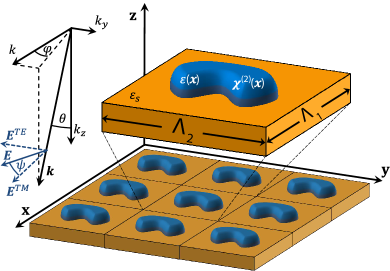
Figure 1: Setting for the GSM and closeup of the unit cell of a 2D corrugated grating containing nonlinear material. The grating is described by $\varepsilon({\bf x})$ and ${{\bm{\chi}}^{(2)}}({\bf x})$ and is under plane wave incidence with wavevector ${\bf k}_{0}$.

Since this analysis does not include nonlinear optical effects in the cover and substrate materials and since the nonlinear polarization ${{\bf P}^{\text{NL}}}({\bf x})$ arises due to a periodically distributed field (7) at the FF, both the external current ${\bf J}^{\text{ext}}=-i\Omega{{\bf P}^{\text{NL}}}$ at the SH and the generalized source term can be expressed as Fourier series,

$${\bf J}^{\text{tot}} = -i\Omega{{\bf P}^{\text{NL}}}-i\Omega(\varepsilon-\varepsilon_{b}){\bf E}$$ (8)

$$= \sum_{n=-\infty}^{\infty}\left[{\bf j}^{\text{NL}}_{n}(z)+{\bf j}^{\mathrm{gen}}_{n}(z)\right]e^{i(k_{nx}x+k_{ny}y)}.$$

The coefficients ${\bf j}^{\text{gen}}_{n}(z)$ depend on all field terms ${\bf E}_{m}(z)$

$${\bf j}^{\text{gen}}_{n}(z) = -i\omega\left\{\left[\varepsilon(z)-\varepsilon_{b}(z)\right]{\bf E}(z)\right\}_{n}$$

$$= -i\omega\sum_{m=-\infty}^{\infty}\left[\varepsilon(z)-\varepsilon_{b}(z)\right]_{n-m}{\bf E}_{m}(z).$$

The solution operator ${{\bf N}_{b}}$ for a periodic source current, ${\bf j}_{n}(z)e^{i(k_{nx}x+k_{ny}y)}$, in homogeneous space with constant permittivity $\varepsilon_{b}$ reads st12jqsrt ; s87josab :

$${\bf E}_{n}(z)=\frac{i}{\omega}\int{\bf G}_{n}(z,z^{\prime}){\bf j}_{n}(z^{\prime})dz^{\prime},$$ (9)

with the tensor Green’s function

$${\bf G}_{n}(z,z^{\prime})= \left({{\bf e}^{+}_{n}}{{\bf e}^{+}_{n}}^{T}+{\bf h}^{+}_{n}{{\bf h}^{+}_{n}}^{T}\right){H}(z\vbox{ \hrule width=3.33333pt,height=0.0pt}z^{\prime})e^{i\kappa^{b}_{nz}(z\vbox{ \hrule width=2.33333pt,height=0.0pt}z^{\prime})}$$

$$+ \left({{\bf e}^{-}_{n}}{{\bf e}^{-}_{n}}^{T}+{\bf h}^{-}_{n}{{\bf h}^{-}_{n}}^{T}\right){H}(z^{\prime}\vbox{ \hrule width=3.33333pt,height=0.0pt}z)e^{i\kappa^{b}_{nz}(z^{\prime}\vbox{ \hrule width=2.33333pt,height=0.0pt}z)}$$

$$- \varepsilon_{b}^{-1}{\bf e}_{z}{\bf e}_{z}^{T}\delta(z-z^{\prime}).$$ (10)

Here, ${\bf e}_{n}^{\pm}$ and ${\bf h}_{n}^{\pm}$ are TE and TM component vectors, respectively, of the $n^{\text{th}}$ Fourier term of the electric field ${\bf E}_{n}$, $H(\cdot)$ denotes the Heaviside step function, and $\mathbf{a}^{T}$ means the transpose of a vector $\mathbf{a}$. The unit vector in $z$-direction is denoted by ${\bf e}_{z}$. Also, the dispersion relation $\kappa^{b}_{nz}=\left[\mu_{0}\varepsilon_{b}\omega^{2}-(k_{nx})^{2}-(k_{ny})^{2}\right]^{1/2}$ holds. One can see that the tensor ${\bf G}_{n}$ gives rise to upwards and downwards propagating plane waves and a stationary term. In order to express the solution in terms of a superposition of plane waves, we eliminate the contribution of the $\delta$-term in Eq. (10) by defining the modified electric field

$$\tilde{E}_{\alpha}(z)=E_{\alpha}(z)-\frac{\delta_{\alpha,z}}{i\omega\varepsilon_{b}}J_{\alpha}^{\text{tot}}(z).$$ (11)

The Fourier components of this modified field, $\tilde{\bf E}_{n}(z)=\textsf{Q}_{n}{\bf a}_{n}(z)$, can be expressed via their TE/TM amplitudes, ${\bf a}_{n}(z)=\left(a_{en}^{+}(z),a_{en}^{-}(z),a_{hn}^{+}(z),a_{hn}^{-}(z)\right)$, and the matrix $\textsf{Q}_{n}=\left({\bf e}_{n}^{+},{\bf e}_{n}^{-},{\bf h}_{n}^{+},{\bf h}_{n}^{-}\right)$. Additionally, Eq. (11) leads to a useful property of its $z$-component:

$$\tilde{E}_{z}(z)=\frac{D_{z}}{\varepsilon_{b}}.$$ (12)

The total source can be rewritten as

$${\bf J}^{\text{tot}} = {\bf J}^{\text{ext}}+{\bf J}^{\text{gen}}({\bf E})={\bf J}^{\text{ext}}-i\omega(\varepsilon{\bf E}-\varepsilon_{b}{\bf E})$$ (13)

$$= -i\omega({\bf P}^{\text{NL}}+\varepsilon{\bf E}-\varepsilon_{b}{\bf E})=-i\omega\left({\bf D}-{\bf D}_{b}\right),$$

where ${\bf D}_{b}=\varepsilon_{b}{\bf E}$ and ${\bf P}^{\text{NL}}=0$ if $\omega=\omega_{0}$. So far, an infinite number of terms in the Fourier series was considered. However, it is well known (lm96josaa ; l96josaa ; l97josaa ) that the factorization of products of periodic functions with a finite number of terms has to be performed with care, namely the correct approach is dictated by the continuity properties of the factors in the product. To be more specific, products of functions with non-simultaneous discontinuities (e.g., the tangential component of the electric displacement field $D_{\parallel}=\varepsilon E_{\parallel}+P^{\text{NL}}_{\parallel}$) can be factorized using Laurent’s product rule, whereas continuous products of functions with simultaneous discontinuities (the normal component $D_{\perp}=\varepsilon E_{\perp}+P^{\text{NL}}_{\perp}$ is continuous at interfaces, whereas $\varepsilon$ and $E_{\perp}$ can be discontinuous) can be factorized using the inverse rule. In the context of numerical methods for periodic structures in the Fourier space, such as the FMM and GSM, the violation of the correct factorization rules causes slow convergence with respect to the number of retained diffraction orders. In contrast to previous work wgp14spie , where the correct factorization was only used in the linear part of the calculations, we now show how the correct factorization should be implemented in the nonlinear part of the calculations.

We now present the derivation of this modified rule and the impact of its correct application on the accuracy of the calculations is investigated in Section III. Thus, to illustrate why a modified factorization rule for the inhomogeneous wave equation is necessary, we consider the example given in l96josaa , adapted to our case:

$$f(x) = \left\{\begin{array}[]{ll}a,&|x|<\pi/2,\\ a/2,&|x|\geq\pi/2,\end{array}\right.$$

$$p(x) = 0.1c[1+\sin(x)]+\left\{\begin{array}[]{ll}c,&|x|<\pi/2,\\ 0,&|x|\geq\pi/2,\end{array}\right.$$

$$g(x) = -\frac{p(x)}{f(x)}+\left\{\begin{array}[]{ll}b(1-|x|/\pi),&|x|<\pi/2,\\ 2b(1-|x|/\pi),&|x|\geq\pi/2,\end{array}\right.$$

$$d(x) = f(x)g(x)+p(x).$$

Here, $a,b>0$ and $c\geq 0$ are arbitrary constants. One can easily see that the function $d$ is continuous, whereas $f$ and $g$ have concurrent discontinuities at $|x|=\pi/2$. For $c\neq 0$, $p$ is also discontinuous at $|x|=\pi/2$. Otherwise, Li’s example l96josaa is obtained. Figure 2(a) shows the functions for $a=6$, $b=2$, and $c=3$.

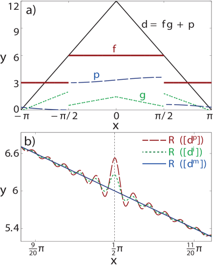
Figure 2: a) Discontinuous functions $f$ (thick brown), $g$ (dashed green), and $p$ (broken blue lines) and continuous function $d$ (solid black), for $a=6$, $b=2$, $c=3$. b) Reconstruction of Fourier series with $200$ components around discontinuity obtained by the product rule (broken brown lines), inverse rule (dashed green), and modified inverse rule (solid blue).

In order to obtain the vector, ${\left[d\right]}$, of Fourier coefficients of $d$, three different factorizations are compared, the results being depicted in Fig. 2(b). The product rule yields ${\left[d^{p}\right]}={\left\llbracket f\right\rrbracket}{\left[g\right]}+{\left[p\right]}$, where ${\left\llbracket f\right\rrbracket}$ is the Toeplitz matrix of the Fourier coefficients of $f$. The reconstruction, ${{\bf R}\left({\left[d^{p}\right]}\right)}$, of the function $d$ shows strong oscillations at $|x|=\pi/2$ around the expectedly continuous function $d$ itself. The reason for this behavior is that the product rule propagates the overshoot from ${{\bf R}\left({\left[f\right]}\right)}$ and ${{\bf R}\left({\left[g\right]}\right)}$ to the reconstruction of the product ${{\bf R}\left({\left\llbracket f\right\rrbracket}{\left[g\right]}\right)}$. In addition, the oscillatory behavior of ${{\bf R}\left({\left[p\right]}\right)}$ at $|x|=\pi/2$ adds to the variations of the reconstructed product, ${{\bf R}\left({\left[d^{p}\right]}\right)}$.

A direct application of the inverse rule for the product yields ${\left[d^{i}\right]}={\left\llbracket 1/f\right\rrbracket}^{-1}{\left[g\right]}+{\left[p\right]}$. The oscillations of the reconstruction ${{\bf R}\left({\left[d^{i}\right]}\right)}$ are now less pronounced but still consist of additive contributions from both terms ${{\bf R}\left({\left\llbracket 1/f\right\rrbracket}^{-1}{\left[g\right]}\right)}$ and ${{\bf R}\left({\left[p\right]}\right)}$.

We propose a modification of the product rule: we rewrite the continuous function $d(x)=f(x)g(x)+p(x)=f(x)\big{[}g(x)+p(x)/f(x)\big{]}$ as a product of discontinuous functions in the space-domain. The two factors have complementary discontinuities, whence the inverse rule applied to this product yields the correct factorization, ${\left[d^{m}\right]}={\left\llbracket 1/f\right\rrbracket}^{-1}\left({\left[g\right]}+{\left[p/f\right]}\right)$. This is illustrated by the reconstruction ${{\bf R}\left({\left[d^{m}\right]}\right)}$, which shows no spurious oscillations at the points of discontinuity.

Armed with this correct factorization rule, let us now consider Eq. (13). Thus, we find that in the context of the nonlinear GSM, $d$, $f$, $g$, and $p$ correspond to the continuous normal component of the displacement field, $D_{\perp}$, the permittivity, $\varepsilon$, $E_{\perp}$, and $P^{\text{NL}}_{\perp}$, respectively. The correct factorization of tangential and parallel components of ${\bf D}$ therefore reads:

$${\left[D_{\parallel}\right]} ={\left\llbracket\varepsilon\right\rrbracket}{\left[E_{\parallel}\right]}+{\left[P^{\text{NL}}_{\parallel}\right]},$$ (17a)

$${\left[D_{\perp}\right]} ={\left\llbracket 1/\varepsilon\right\rrbracket}^{-1}\left({\left[E_{\perp}\right]}+{\left[P^{\text{NL}}_{\perp}/\varepsilon\right]}\right).$$ (17b)

We specify again that ${\left[V\right]}$ denotes the vector of $N_{o}=(2N_{1}+1)(2N_{2}+1)$ Fourier coefficients of $V$. The truncation of Fourier terms with $n_{1}=-N_{1},\ldots,N_{1}$ and $n_{2}=-N_{2},\ldots,N_{2}$, with $N_{1}$ and $N_{2}$ integers, corresponds to a rectangular truncation pattern in the Fourier space. Problem specific, non-rectangular patterns could also be used and may lead to faster convergence in certain cases (see l97josaa for a study of different truncation patterns in the FMM). Accordingly, the Fourier coefficients of the total source current, ${\bf j}_{n}={\bf j}_{n}^{\text{NL}}+{\bf j}_{n}^{\text{gen}}$, defined by Eq. (8) are given by

$${\left[j_{\parallel}\right]} = -i\omega\varepsilon_{b}\left\{\left({\left\llbracket\frac{\varepsilon}{\varepsilon_{b}}\right\rrbracket}-\textsf{I}\right){\left[E_{\parallel}\right]}+\varepsilon_{b}^{-1}{\left[P^{\text{NL}}_{\parallel}\right]}\right\},$$

$${\left[j_{\perp}\right]} = -i\omega\varepsilon_{b}\left\{\left({\left\llbracket\frac{\varepsilon_{b}}{\varepsilon}\right\rrbracket}^{-1}\!\!\!\!-\textsf{I}\right){\left[E_{\perp}\right]}+{\left\llbracket\frac{\varepsilon_{b}}{\varepsilon}\right\rrbracket}^{-1}{\left[P^{\text{NL}}_{\perp}/\varepsilon\right]}\right\},$$

where I denotes the identity matrix of respective size.

It remains to reformulate these equations, which are given in terms of the $(\perp,\parallel)$-components of ${\bf E}$, in terms of the Cartesian components of $\tilde{\bf E}$, the latter ones being the actual variables used in the GSM formalism. To this end, a local normal/tangential vector field is defined so that for any vectorial quantity $\bf v$ we can write:

$$\left(\begin{array}[]{c}v_{x}\\ v_{y}\\ v_{z}\end{array}\right)=\textsf{B}\left(\begin{array}[]{c}v_{n}\\ v_{\psi}\\ v_{\phi}\end{array}\right),$$

where the orthogonal transformation matrix

$$\textsf{B}=\left(\hat{\mathbf{n}},\hat{\mathbf{\psi}},\hat{\mathbf{\phi}}\right)=\left(\begin{array}[]{ccc}\cos\phi\sin\psi&\cos\phi\cos\psi&-\sin\phi\\ \sin\phi\sin\psi&\sin\phi\cos\psi&\cos\phi\\ \cos\psi&-\sin\psi&0\end{array}\right)$$

is a concatenation of the unit vectors in normal, and both tangential directions $\hat{\bf n}$, $\hat{\mathbf{\psi}}$, and $\hat{\mathbf{\phi}}$, respectively. Using this transformation we get (analogously to Appendix A in st12jqsrt ):

$${\left[j_{\alpha}\right]}=-i\omega\varepsilon_{b}\sum_{\beta}\left(\Delta\delta_{\alpha\beta}-\textsf{D}\Gamma_{\alpha\beta}\right){\left[E_{\beta}\right]}-i\omega\varepsilon_{b}{\left[\bar{p}_{\alpha}^{p}\right]},\ \ \ \$$ (20)

where

$$\left(\begin{array}[]{c}{\left[\bar{p}^{p}_{x}\right]}\\ {\left[\bar{p}^{p}_{y}\right]}\\ {\left[\bar{p}^{p}_{z}\right]}\end{array}\right)=\textsf{B}\ \mathrm{diag}\left({\left\llbracket\frac{\varepsilon_{b}}{\varepsilon}\right\rrbracket}^{-1},\varepsilon_{b}^{-1},\varepsilon_{b}^{-1}\right)\left(\begin{array}[]{c}{\left[p^{p}_{n}/\varepsilon\right]}\\ {\left[p^{p}_{\psi}\right]}\\ {\left[p^{p}_{\phi}\right]}\end{array}\right).$$

The matrices $\Delta$ and D are defined as

$$\Delta={\left\llbracket\frac{\varepsilon}{\varepsilon_{b}}\right\rrbracket}-\textsf{I}\quad\text{and}\quad\textsf{D}={\left\llbracket\frac{\varepsilon}{\varepsilon_{b}}\right\rrbracket}-{\left\llbracket\frac{\varepsilon_{b}}{\varepsilon}\right\rrbracket}^{-1}$$

and $\Gamma_{\alpha\beta}$ are the Fourier images of the entries of the matrix

$$\!\Gamma(z)\!=\!\!\left(\!\!\begin{array}[]{ccc}\cos^{2}\!\phi\sin^{2}\!\psi&\sin\phi\cos\phi\sin^{2}\!\psi&\cos\phi\sin\psi\cos\psi\\ \sin\phi\cos\phi\sin^{2}\!\psi&\sin^{2}\!\phi\sin^{2}\!\psi&\sin\phi\sin\psi\cos\psi\\ \cos\phi\sin\psi\cos\psi&\sin\phi\sin\psi\cos\psi&\cos^{2}\!\psi\end{array}\!\!\right)\!\!.$$

In agreement with the modified factorization rule, the Fourier series coefficients ${\left[p^{p}_{n}/\varepsilon\right]}$ are obtained by numerical integration of the space-domain quotient of the functions $p^{p}_{n}(x)$ and $\varepsilon(x)$.

In order to eliminate ${\bf E}$ in favor of $\tilde{\bf E}$ we insert

$$\frac{{\left[j_{z}\right]}}{i\omega\varepsilon_{b}}=\textsf{D}\left(\Gamma_{zx}{\left[E_{x}\right]}+\Gamma_{zy}{\left[E_{y}\right]}\right)+\left(\textsf{D}\Gamma_{zz}-\Delta\right){\left[E_{z}\right]}-{\left[\bar{p}^{p}_{z}\right]}$$

into the definition (11) of $\tilde{\bf E}$ to obtain

$$\tilde{{\left[E_{z}\right]}}=-\textsf{D}\left(\Gamma_{zx}{\left[E_{x}\right]}+\Gamma_{zy}{\left[E_{y}\right]}\right)+\textsf{C}E_{z}+{\left[\bar{p}^{p}_{z}\right]},$$

where $\textsf{C}=\Delta-\textsf{D}\Gamma_{zz}$. This yields ${\left[{\bf E}\right]}$ resolved in terms of $\tilde{{\left[{\bf E}\right]}}$, which in matrix form is expressed as

$$\left(\begin{array}[]{c}{\left[E_{x}\right]}\\ {\left[E_{y}\right]}\\ {\left[E_{z}\right]}\end{array}\right) = \left(\begin{array}[]{ccc}\textsf{I}&0&0\\ 0&\textsf{I}&0\\ \textsf{C}^{-1}\textsf{D}\Gamma_{zx}&\textsf{C}^{-1}\textsf{D}\Gamma_{zy}&\textsf{C}^{-1}\end{array}\right){\left(\begin{array}[]{c}\tilde{{\left[E_{x}\right]}}\\ \tilde{{\left[E_{y}\right]}}\\ \tilde{{\left[E_{z}\right]}}\end{array}\right)}$$ (32)

$$- \left(\begin{array}[]{c}0\\ 0\\ \textsf{C}^{-1}{\left[\bar{p}^{p}_{z}\right]}\end{array}\right).$$ (36)

Plugging this formula back into Eq. (20) provides the total source current, which consists of the generalized source dependent on the unknown field $\tilde{\bf E}$ and a physical source whose origin is the known polarization:

$$\frac{{\left[j_{\alpha}\right]}}{i\omega\varepsilon_{b}}=\sum_{\beta}\textsf{W}_{\alpha\beta}\tilde{{\left[E_{\beta}\right]}}+{\left[\tilde{p}_{\alpha}^{p}\right]},$$ (37)

where the modified polarization reads

$${\left[\tilde{p}_{\alpha}^{p}\right]} = -{\left[\bar{p}^{p}_{\alpha}\right]}+\left(\Delta\delta_{\alpha z}-\textsf{D}\Gamma_{\alpha z}\right)\textsf{C}^{-1}{\left[\bar{p}^{p}_{z}\right]}$$ (38)

and the matrix $\textsf{W}(z)$ is defined as

$$\textsf{W}=\left({\begin{array}[]{ccc}\textsf{N}_{xx}+\textsf{D}\Gamma_{xx}-\Delta&\textsf{N}_{xy}+\textsf{D}\Gamma_{xy}&\textsf{D}\Gamma_{xz}\textsf{C}^{-1}\\ \textsf{N}_{yx}+\textsf{D}\Gamma_{xx}&\textsf{N}_{xy}+\textsf{D}\Gamma_{yy}-\Delta&\textsf{D}\Gamma_{yz}\textsf{C}^{-1}\\ -\textsf{C}^{-1}\textsf{D}\Gamma_{zx}&-\textsf{C}^{-1}\textsf{D}\Gamma_{zy}&\textsf{C}^{-1}-\textsf{I}\end{array}}\right).$$

Here, $\textsf{N}_{\alpha\beta}=\textsf{D}\Gamma_{\alpha z}\textsf{C}^{-1}\textsf{D}\Gamma_{z\beta}$ combines the geometrical normal field information contained in $\Gamma$ with the physical structure given by $\varepsilon$.

Combining the main results, namely Eq. (37) that expresses the source in terms of $\tilde{\bf E}$ and the Green’s function (9), yields a system of Fredholm integral equations of the second kind for the unknown amplitudes,

$${\bf a}_{n}(z) = {\bf a}^{0}_{n}(z)+\int_{z^{\prime}=0}^{0}pt\textsf{R}_{n}(z,z^{\prime})\sum_{\alpha}\bar{\textsf{Q}}_{:\alpha,n}$$ (39)

$$\times \sum_{m=-N_{o}}^{N_{o}}\sum_{\beta}\textsf{W}_{\alpha\beta,nm}(z^{\prime})\textsf{Q}_{\beta:,m}{\bf a}_{m}(z^{\prime})dz^{\prime},$$

for $n=1,\ldots,N_{o}$, where the sum over $m\equiv(m_{1},m_{2})$ is to be understood as a double finite sum over the integers $m_{1}=-N_{1},\ldots,N_{1}$ and $m_{2}=-N_{2},\ldots,N_{2}$. $\bar{\textsf{Q}}_{:\alpha,n}$ and $\textsf{Q}_{\beta:,m}$ denote the $\alpha$-column and $\beta$-row of $\bar{\textsf{Q}}_{n}$ and $\textsf{Q}_{m}$, respectively. The matrix $\textsf{R}_{n}(z,z^{\prime})\in\mathbb{C}^{4\times 4}$ incorporates the propagation of TE- and TM-polarized, upward and downward plane wave amplitudes of the $n^{\text{th}}$ Fourier component inside the slab-background structure and their reflections at the top and bottom interfaces [see Eqs. (61) and (62) in st12jqsrt for the exact formula]. The known values of ${\bf a}_{n}^{0}(z)$ are either the amplitudes of the incident plane wave electric field in the background structure at the FF or the amplitudes of the external source field ${{\bf N}_{b}}(\mathbf{J}^{\text{ext}})$ at the SH; the latter are given by

$${\bf a}^{0}_{n}(z)=\int_{z^{\prime}=0}^{0}pt\textsf{R}_{n}(z,z^{\prime})\bar{\textsf{Q}}_{n}\tilde{\bf p}^{p}_{n}(z^{\prime})dz^{\prime}.$$ (40)

One can easily see that the modified factorization rule does not affect the generalized source but only changes the external polarization. This means, that all algorithmic enhancements, that make the linear GSM an efficient numerical method, can be applied here as well.

Using the midpoint rule, the system (39) of integral equations is discretized at $N_{l}$ equidistant points, $z_{p}=(p-0.5)0pt/N_{l}$, $p=1,\ldots,N_{l}$. This results in a system of linear equations,

$${\bf a}_{np} = {\bf a}^{0}_{np}+\frac{0pt}{N_{l}}\sum_{q=1}^{N_{l}}\textsf{R}_{n}(z_{p},z_{q})\sum_{\alpha}\bar{\textsf{Q}}_{:\alpha,n}$$ (41)

$$\times \sum_{m=-N_{o}}^{N_{o}}\sum_{\beta}\textsf{W}_{\alpha\beta,nm}(z_{q})\textsf{Q}_{\beta:,m}{\bf a}_{mq},$$

for $n=1,\ldots,N_{0},p=1,\ldots,N_{l}$. The total number of unknowns in Eq. (41) is $4N_{o}N_{l}$ and usually becomes prohibitively large for direct solvers to be used in practical situations of interest.

In order to take full advantage of an iterative solver, the system (41) is reformulated to (see also st12jqsrt ):

$${\bf a}=\left(\textsf{I}+\textsf{R}\bar{\textsf{Q}}\textsf{U}\textsf{A}^{-1}\textsf{Q}\right){\bf a}^{0},$$ (42)

where ${\bf a}$ and ${\bf a}^{0}$ are the vectors containing the discrete unknowns, ${\bf a}_{np}={\bf a}_{n}(z_{p})$, and the known amplitudes, ${\bf a}^{0}_{np}={\bf a}^{0}_{n}(z_{p})$, respectively, $\textsf{A}=\textsf{M}-\textsf{QR}\bar{\textsf{Q}}\textsf{U}$, and $\bar{\textsf{Q}}$ and Q are block-diagonal matrices with $\bar{\textsf{Q}}_{n}$ and $\textsf{Q}_{n}$ on their block-diagonal, respectively. The matrix $\textsf{R}\in\mathbb{C}^{4N_{o}N_{l}\times 4N_{o}N_{l}}$ corresponds to $\textsf{R}_{n}(z_{p},z_{q})$: Its $\big{(}4(n-1)N_{l}+4(p-1)+[1,..,4],\ 4(n-1)N_{l}+4(q-1)+[1,..,4]\big{)}$-entries are given by $\textsf{R}_{n}(z_{p},z_{q})$. Hence, R is diagonal with respect to the Fourier component $n$ and has Toeplitz-structure with respect to the layer indices $p$ and $q$. The matrices

$$\textsf{M}=\left(\!\!\begin{array}[]{ccc}{\left\llbracket\frac{\varepsilon_{b}}{\varepsilon}\right\rrbracket}{\left\llbracket\frac{\varepsilon}{\varepsilon_{b}}\right\rrbracket}&0&0\\ 0&{\left\llbracket\frac{\varepsilon_{b}}{\varepsilon}\right\rrbracket}{\left\llbracket\frac{\varepsilon}{\varepsilon_{b}}\right\rrbracket}&0\\ 0&0&{\left\llbracket\frac{\varepsilon}{\varepsilon_{b}}\right\rrbracket}{\left\llbracket\frac{\varepsilon_{b}}{\varepsilon}\right\rrbracket}\end{array}\!\!\right)\small\sin^{2}\psi+\cos^{2}\psi,$$ (46)

$$\textsf{F}=\textsf{I}-{\left\llbracket\frac{\varepsilon_{b}}{\varepsilon}\right\rrbracket}{\left\llbracket\frac{\varepsilon}{\varepsilon_{b}}\right\rrbracket},~{}~{}~{}\textsf{G}=\textsf{I}-{\left\llbracket\frac{\varepsilon}{\varepsilon_{b}}\right\rrbracket}{\left\llbracket\frac{\varepsilon_{b}}{\varepsilon}\right\rrbracket},$$

$$\textsf{U}=\left(\!\!\begin{array}[]{ccc}\Delta\textsf{M}_{xx}+\textsf{G}{\left\llbracket\frac{\varepsilon}{\varepsilon_{b}}\right\rrbracket}\Gamma_{xx}\!\!\!&\textsf{G}{\left\llbracket\frac{\varepsilon}{\varepsilon_{b}}\right\rrbracket}\Gamma_{xy}&\textsf{G}\Gamma_{xz}\\ \textsf{G}{\left\llbracket\frac{\varepsilon}{\varepsilon_{b}}\right\rrbracket}\Gamma_{yx}&\!\!\!\Delta\textsf{M}_{yy}+\textsf{G}{\left\llbracket\frac{\varepsilon}{\varepsilon_{b}}\right\rrbracket}\Gamma_{yy}&\textsf{G}\Gamma_{yz}\\ \textsf{F}\Gamma_{zx}&\textsf{F}\Gamma_{zy}&\!\!\textsf{M}_{zz}-{\left\llbracket\frac{\varepsilon_{b}}{\varepsilon}\right\rrbracket}\end{array}\!\!\right),$$ (50)

are defined such that $\textsf{W}=\textsf{UM}^{-1}$ but they do not contain inverted submatrices themselves. Additionally, U and M are block-Toeplitz-Toeplitz-matrices with respect to the index pair $n=(n_{1},n_{2})$. Due to the Toeplitz-property of its submatrices, multiplication of a vector ${\bf b}$ of size $3N_{o}N_{l}$ with the $3N_{o}N_{l}\times 3N_{o}N_{l}$ system matrix A can be performed in $\mathcal{O}(N_{o}N_{l}\log(N_{o})\log(N_{l}))$ blahut85aw operations instead of $\mathcal{O}(N_{o}^{2}N_{l}^{2})$ for the standard matrix-vector multiplication. Therefore, the use of an iterative solver based on matrix-vector multiplications like GMRES is highly beneficial. Although the reformulation Eq. (42) removes all inverted submatrices from the system matrix A itself, the evaluation of the modified source polarization ${\left[\tilde{\bf p}^{p}\right]}$ in Eq. (38) still requires a one-time inversion of matrix C. In practice, the computational cost of this nonrecurring inversion is, however, negligible compared to the overall runtime of the algorithm, which is dominated by the inversion-free iterative solution process.

III Numerical analysis and convergence studies

In this section we examine the convergence and runtime properties of the linear and nonlinear parts of the GSM using cylindrical gratings as test examples 2D made either of dielectric or metallic materials. Importantly, we illustrate the impact of the application of the correct factorization rule as compared to the old factorization.

The unit cell of the grating under consideration is assumed to be rectangular and, for simplicity, the two periods are set to be equal, $\Lambda_{1}=\Lambda_{2}=\Lambda=$ $2\text{\,}\mathrm{\SIUnitSymbolMicro m}$. It contains a cylindrical disk of height, $h=$ $200\text{\,}\mathrm{nm}$, and radius, $r=0.25\Lambda=$ $500\text{\,}\mathrm{nm}$. The disk and substrate have refractive index, $n_{s}=2$, whereas the cover region is vacuum with $n_{c}=1$. We assume an isotropic nonlinear susceptibility tensor, $\chi^{(2)}_{jkl}=\bar{\chi}\delta_{jk}\delta_{kl}$, with $\bar{\chi}=$ ${10}^{-8}\text{\,}\mathrm{m}\text{\,}{\mathrm{V}}^{-1}$. The incident plane wave at the fundamental wavelength of $\lambda_{\mathrm{FF}}=$ $1.5\text{\,}\mathrm{\SIUnitSymbolMicro m}$, is specified by the angles $\theta=$ $30\mathrm{°}$ and $\phi=$ $70\mathrm{°}$, and a $\psi=$ $45\mathrm{°}$ polarization.

The optical response of the device at the FF and SH is computed by the linear and nonlinear GSM, respectively. We perform simulations for an increasing number of diffraction orders $N_{o}=(2N_{1}+1)(2N_{2}+1)$ for $N_{1}=N_{2}\in\{3,5,...,23\}$ and increasing number of layers, $N_{l}\in\{12,25,50,...,400\}$. In order to assess the efficiency of the algorithm, we compute the following quantities: the reflection and transmission coefficients, $R^{FF/SH}$ and $T^{FF/SH}$, respectively, at the FF/SH, the number $N_{\text{iter}}^{FF}$ and $N_{\text{iter}}^{SH}$ of GMRES iterations necessary to solve Eq. (42) at the FF and SH, respectively, and the GSM runtime needed to complete the linear ($t^{FF}$) and nonlinear ($t^{SH}$) part of the computations.

For the validation of the linear calculations results, they are compared to data obtained by using an efficient normal vector field formulation srk07josaa of the FMM, which is also commercially available omnircwaPD . For the presented comparison, both methods were implemented in MATLAB and all simulations were performed on a single $2.5\text{\,}\mathrm{GHz}$ processor to allow a fair comparison of simulation times.

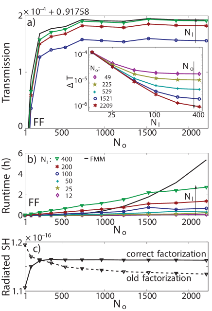
Figure 3: a) Transmission efficiency obtained using GSM for increasing $N_{l}$ [colors, legend from b)] and FMM (black). Inset: discretization error of GSM vs. $N_{o}$. b) Runtime of GSM for increasing $N_{l}$ (colors) and of FMM (black). c) Convergence behavior of radiated SH in the direction of the incoming plane wave using the two different factorization rules.

The results of this analysis are summarized in Fig. 3. The dependence of the transmission coefficient at the FF, $T^{FF}$, on the number of diffraction orders, computed by using the GSM for several values of the numbers of layers $N_{l}$ in which the grating is divided, is presented in Fig. 3(a). For comparison, we present the same dependence determined by using the FMM. Both methods show a similar convergence pattern with respect to $N_{o}$ and the computed transmission coefficient rapidly approaches the asymptotic value of $T^{FF}=0.917772$. For the investigated lossless device the GSM conserves the incoming optical power up to a relative error of $10^{\vbox{ \hrule width=2.33333pt,height=0.0pt}5}$ for low $N_{o}<1000$ and the power conservation improves to $10^{\vbox{ \hrule width=2.33333pt,height=0.0pt}6}$ as $N_{o}$ further increases.

The inset in Fig. 3(a) illustrates the error in the transmission due to the discretization of the integral equation, defined as $\Delta T=T^{FF}-T^{FF}_{FMM}$, calculated for several values of orders, $N_{o}\in\{49,...,2209\}$, and for increasing $N_{l}$. Given sufficiently many orders, e.g. $N_{o}=2209$, quadratic decrease of $\Delta T$ is achieved, which is to be expected since using the midpoint rule in the discretization of the integral equation implies quadratic convergence. For smaller $N_{o}$, e.g. $N_{o}=225$, the convergence plateaus at a small number of layers. This is because the reformulated linear system (42), which enables the use of the accelerated matrix-vector multiplication, is only $N_{o}$-asymptotically equivalent to the original system (41).

Figure 3(b) depicts the runtime $t^{FF}$ necessary to compute the solution of the problem at the FF for increasing $N_{o}$ and for different $N_{l}$. The linear GSM exhibits nearly optimal runtime as $t^{FF}$ increases log-linearly with both $N_{o}$ and $N_{l}$. This is because $t^{FF}$ is chiefly determined by the computational work needed to iteratively find the solution of Eq. (42) using GMRES, which in turn depends on the number of iterations $N_{\text{iter}}^{FF}$ and, if $N_{\text{iter}}^{FF}\ll N_{o}N_{l}$, on the time required for the system-matrix vector multiplication; this latter quantity is of order $\mathcal{O}(N_{o}N_{l}\log(N_{o})\log(N_{l}))$. For the investigated device, only $N_{\text{iter}}^{FF}=39$ GMRES iterations are necessary to solve Eq. (42), where $N_{\text{iter}}^{FF}$ is nearly independent of $N_{o}$ and $N_{l}$ (see also Table 1, second row). The black line in Fig. 3(b) indicates the runtime of the FMM, $t^{FF}_{FMM}$, which follows a $\mathcal{O}(N_{o}^{3})$ dependence. This is the expected behavior as the FMM involves finding the solution of an eigenproblem of size $N_{o}$. The asymptotic advantage of the GSM becomes evident, e.g. at $N_{l}=200$, where for $N_{o}=1225$, $t^{FF}_{FMM}$ becomes larger than $t^{FF}$.

For the computations at the SH, the GSM computational time still follows the $\mathcal{O}(N_{o}N_{l}\log(N_{o})\log(N_{l}))$ trend; however, as compared to the FF, approximately $3\times$ more iterations, $N_{\text{iter}}^{SH}=100$, are necessary to solve Eq. (42) at the SH. We identify two possible reasons for this behavior: First, we found that for plane wave excitation, the smaller the wavelength the more iterations were necessary for GMRES to solve Eq. (42) and second, both the r.h.s. of this equation and its solution are more inhomogeneous at the SH as compared to the FF.

The results for the generated SH, computed with $N_{l}=400$, are depicted in Fig. 3(c). Specifically, this figure shows the radiated power at the SH in the direction of the incoming wave, normalized to the incident power at the FF. The data corresponding to the solid line was obtained by using the modified inverse rule for the source polarization and shows remarkably fast convergence to a value of $T^{SH}=1.163\cdot 10^{\vbox{ \hrule width=2.33333pt,height=0.0pt}16}$ with increasing $N_{o}$. By contrast, when using the unmodified rule $T^{SH}$ does not reach its asymptotic value even for as many as $N_{o}=2209$ orders, despite the fact that the FF solution is already converged if $N_{o}\gtrsim 750$ [see Fig. 3(a)]. Note that the old and correct factorizations tend to slightly different values. Such a behavior has already been reported for linear calculations in the FMM (l97josaa ).

Table 1: Characteristics of the nonlinear GSM for dielectric and lossy materials

$n$	$N_{\text{iter}}^{FF}$	$N_{\text{iter}}^{SH}$	$T^{FF}$	$A^{FF}$	​​​—​​​​​ $T^{SH}$ ​​​—​​​​​
1.45	​​​—​​​​​ $2.88\cdot 10^{\vbox{ \hrule width=2.33333pt,height=0.0pt}17}$ ​​​—​​​​​	38	0.972998	$2.6\cdot 10^{\vbox{ \hrule width=2.33333pt,height=0.0pt}8}$
2	​​​—​​​​​ $1.16\cdot 10^{\vbox{ \hrule width=2.33333pt,height=0.0pt}17}$ ​​​—​​​​​	100	0.917772	$8.0\cdot 10^{\vbox{ \hrule width=2.33333pt,height=0.0pt}7}$
3	​​​—​​​​​ $4.57\cdot 10^{\vbox{ \hrule width=2.33333pt,height=0.0pt}18}$ ​​​—​​​​​	400	0.825020	$5.8\cdot 10^{\vbox{ \hrule width=2.33333pt,height=0.0pt}6}$
$1.5\!+\!1i$	96	157	0.620149	0.283418	​​​—​​​​​ $7.41\cdot 10^{\vbox{ \hrule width=2.33333pt,height=0.0pt}19}$ ​​​—​​​​​
$0.36\!+\!6.5i$	2160	1968	0.381113	0.193255	​​​—​​​​​ $5.99\cdot 10^{\vbox{ \hrule width=2.33333pt,height=0.0pt}18}$ ​​​—​​​​​

Finally, we investigated the convergence properties of the GSM when it was applied to simulate diffraction gratings made of three different lossless dielectric materials, a lossy dielectric, and metallic components. The results, shown in Table 1, provide valuable insights into the characteristics of the GSM. Thus, clear trends can be observed in the case of lossless dielectric gratings: the higher the refractive index $n$ is the more GMRES iterations $N_{\text{iter}}^{FF}$ are necessary at the FF and the number of iterations $N_{\text{iter}}^{SH}$ at the SH increases faster than $N_{\text{iter}}^{FF}$. The numerical absorption, $A^{FF}=1-T^{FF}-R^{FF}$, which in the case of gratings made of lossless materials quantifies the degree to which the algorithm conserves the energy, decreases with the index of refraction. The lossy material with $n=1.5+i$ can be efficiently analyzed by the GSM: the $N_{\text{iter}}^{FF}$ is relatively small and increases only by 50% for the calculation of the SH electromagnetic field.

The metallic grating requires a more detailed discussion. The derivation of the GSM formally allows complex values of the permittivity $\varepsilon({\bf x})$ and the algorithm’s implementation does show that the method can be applied to simulate diffraction by lossy structures (see the $n=1.5+i$ example in Table 1). However, we found out that the very large number of required GMRES iterations makes the method particularly slow when applied to structures containing very lossy components, namely a material with $n=0.36+6.5i$. We also found out that for metals $N_{\text{iter}}$ increases strongly when $N_{o}$ increases (the presented results for $n=0.36+6.5i$ are for $N_{o}=529$; increasing $N_{o}$ would require $N_{\text{iter}}>5000$ to achieve convergence of GMRES). Summing up these results, the GSM in the presented form is most efficient and most suitable for shallow, low refractive index contrast, dielectric devices. However, an improvement of the GSM using curvilinear coordinates st13oe allows one to efficiently calculate metallic structures as well but we have not implemented this version of the algorithm in the nonlinear case.

IV Application to SHG in textured slab waveguides

In this section we illustrate the versatility of our method by showing how it can be applied to a problem of practical importance, namely to the maximization of the SHG in a phase-matched configuration. Because of the weak nature of nonlinear optical interactions, the radiated SH in practical settings is orders of magnitude smaller than the linear excitation. Therefore field enhancing mechanisms are particularly important in this context as they can be employed to increase the efficiency of SHG in practical applications. To this end, we consider the SHG in a diffraction grating resonantly coupled to a slab waveguide, both optical devices being made of quadratically nonlinear optical materials.

To add specificity to our problem, we assume that the nonlinear material in the device is GaAs (refractive index $n=3.4$), which due to its large optical nonlinearity is a particularly suitable choice for our device application. It crystallizes in the zincblende lattice type, so that it belongs to the crystal point group $\bar{4}3m$. Hence, the non-vanishing components of its second-order susceptibility tensor are $\chi^{(2)}_{xyz}=\chi^{(2)}_{xyz}=\chi^{(2)}_{yxz}=\chi^{(2)}_{yzx}=\chi^{(2)}_{zxy}=\chi^{(2)}_{zyx}=$ $7.4\text{\times}{10}^{-10}\text{\,}\mathrm{m}\text{\,}{\mathrm{V}}^{-1}$ b08ap , which is a relatively large value as compared to that of most other non-centrosymmetric materials. As substrate we choose CaF₂ ($n_{s}=1.4$) and consider air ($n_{c}=1$) as cover, which provides the high refractive index contrast needed to achieve good field confinement in the slab waveguide.

In order for the incident plane waves to couple and interact with the slab waveguide modes a periodic optical grating that breaks the translational symmetry of the structure is placed on top of the waveguide. As a result the propagation constant, $\beta_{\nu}(\lambda)$, of the $\nu$th slab waveguide mode is folded within the first Brillouin zone of the grating. When the difference between the tangential component of the incident wavevector, ${\bf k}_{\parallel}$, and the propagation constant $\beta_{\nu}(\lambda)$ is equal to a multiple of the grating vector this waveguide mode can be resonantly excited. In particular, one expects to observe strong field enhancement in the slab waveguide at the corresponding resonance wavelengths and consequently significantly stronger nonlinear optical interaction, an effect that has been recently used to demonstrate enhanced optical absorption in such optical devices po07ol .

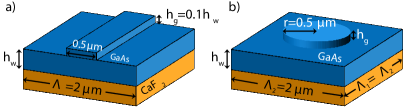
Figure 4: a) Unit cell of a one-dimensional binary grating and b) two-dimensional cylindrical grating on top of a slab waveguide made of nonlinear GaAs on a CaF₂ substrate.

In the context of SHG there are two kinds of resonances that can affect the nonlinear optical response of the device: linear resonances correspond to the grating-induced, resonant excitation of a waveguide mode at the FF by a plane wave incident at a certain angle and wavelength, $\lambda_{FF}$. We expect then that the optical field at the FF is strongly enhanced and confined inside the waveguide, thus a stronger nonlinear polarization is created, which in turn excites a stronger field at the SH wavelength, $\lambda_{SH}=\lambda_{FF}/2$. We call this phenomenon of direct enhancement of the nonlinear response at the SH due to the excitation of a linear resonance at FF an inherited resonance at $\lambda_{SH}$. The second type of nonlinear resonances are intrinsic resonances, which are observed when a waveguide mode is excited at the SH wavelength by the dipoles associated to the nonlinear polarization. In this case the field at the SH is confined inside the waveguide and therefore shows remarkably large radiated SH intensity. Note that the intrinsic resonances are not necessarily grating coupled with the radiative continuum and therefore they can be viewed as nonlinear dark modes of the system bp11n . In particular, one expects that these resonances have large quality factor. We call the inherited and intrinsic resonances nonlinear resonances, since they are observed at the SH. For the sake of simplicity, the modes causing the linear and nonlinear resonances are denoted as linear and nonlinear modes. The SH wavelengths $\lambda_{SH}$ for which both types of nonlinear modes are excited simultaneously are of particular interest because at these wavelengths, this doubly resonant mechanism of SHG, can lead to a remarkably large nonlinear optical response of the device. In the remaining of this section, these ideas are illustrated by studying the nonlinear optical response of 1D and 2D implementations of these devices.

IV.1 One-dimensional binary gratings

We first investigate a 1D grating, which although having a simple structure, provides us the necessary insights to completely understand the more complex 2D design. Thus, let us consider a 1D binary GaAs grating on top of a GaAs slab waveguide, placed onto a CaF₂ substrate, see Fig. 4(a). The height of the slab waveguide, $0pt_{w}$, is a free design parameter and varies from $0.25\text{\,}\mathrm{\SIUnitSymbolMicro m}0.5\text{\,}\mathrm{\SIUnitSymbolMicro m}$. The period of the grating with filling factor $\rho=0.25$ is $\Lambda=$ $2\text{\,}\mathrm{\SIUnitSymbolMicro m}$, the height of the grating region is chosen in relation to the height of the slab waveguide, $0pt_{g}=0.10pt_{w}$.

At the FF, we consider a TM polarized plane wave with wavelength $\lambda_{FF}$ ranging from $3.6\text{\,}\mathrm{\SIUnitSymbolMicro m}4.4\text{\,}\mathrm{\SIUnitSymbolMicro m}$ under $\theta=30^{\circ}$ incidence. By considering the slab waveguide region as homogeneous region of the periodic grating, its nonlinearity is also calculated by the nonlinear GSM. For the calculation of the presented results $N_{o}=21$ diffraction orders and $N_{l}=138,\ldots,275$ GSM-layers were used, each with height of about $2\text{\,}\mathrm{nm}$.

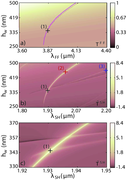
Figure 5: Spectra of transmission coefficient for the binary texture determined for different waveguide heights under normal incidence and for TM polarization. a) Spectra at the fundamental wavelength (pink dispersion curve indicates analytical calculation of $\mathrm{TM}_{0}$ mode). b) Spectra at second harmonic wavelengths (logarithmic scale). c) Zoom-in of the region around a point where an intrinsic and inherited SH resonance dispersion curve cross.

Figure 5(a) shows the transmitted intensity at the FF for a TM polarized incident plane wave with wavelength $\lambda_{FF}$. The spectrum shows a smooth dependence on $\lambda_{FF}$ and $0pt_{w}$, except for a narrow stripe that corresponds to a sharp decrease of the transmission. This change in transmission can clearly be attributed to the excitation of a $\mathrm{TM}_{0}$ waveguide mode. Thus, an analytically calculated resonance wavelength wgp14spie , which is represented by the pink line in the spectrum in Fig. 5(a), is in close proximity to the band of reduced transmission seen in the spectrum. The analytical calculation is obtained for a infinitesimally small perturbation of the slab waveguide, whence the agreement is nearly perfect for low $0pt_{w}$ and slowly deteriorates as $0pt_{w}$ and therefore $0pt_{g}$ increases. Moreover, Fig. 6(a) shows the $y$-component of the magnetic field at the FF, $H_{y}^{FF}$, inside and around the textured waveguide, which is indicated by blue lines, corresponding to the black cross (1) in Fig. 5(a), i.e. to $\lambda_{FF}=$ $3.861\text{\,}\mathrm{\SIUnitSymbolMicro m}$ and $h_{w}=$ $345\text{\,}\mathrm{nm}$. This field profile clearly matches that of the $\mathrm{TM}_{0}$ mode. Note that for a 1D grating under non-conical incidence, the TE and TM components of the electromagnetic field decouple. Accordingly, there is only a single TM mode excited under TM-incidence, in the considered $0pt_{w}$-$\lambda_{FF}$ domain.

In order to better visualize the SHG enhancement, we plot in Fig. 5(b) the logarithm $\tilde{T}^{SH}=\log_{10}T^{SH}$ of the SH intensity, emitted in the direction of the incident wave, for the same incident fundamental field as in Fig. 5(a). The transmission coefficient, $T^{SH}$, is normalized to the SHG in a bulk layer of GaAs having the same volume as the textured grating. This figure clearly shows an increase of the SH intensity due to the excitation of the inherited TM modes and intrinsic TE modes. No intrinsic TM modes are excited in this case. This is due to the particular symmetry properties of ${{\bm{\chi}}^{(2)}}$: for a TM polarized fundamental field ${\bf E}({\bf x})=(E_{x}({\bf x}),0,E_{z}({\bf x}))$, only the $y$-component (i.e. the TE component) of the nonlinear polarization is non-vanishing.

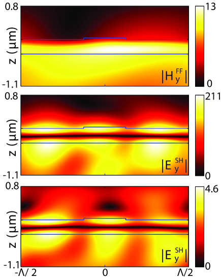
Figure 6: Magnetic and electric field distributions at simultaneous resonance wavelength $\lambda_{FF}=$ $3.45\text{\,}\mathrm{\SIUnitSymbolMicro m}$ for $h_{w}=$ $381\text{\,}\mathrm{nm}$. a) $|H_{y}^{FF}|$ of the fundamental $\mathrm{TM}_{0}$-resonance at the FF. b) $|E_{y}^{SH}|$ of simultaneous resonance at SH. c) $|E_{y}^{SH}|$ of intrinsic $\mathrm{TE}_{1}$ mode at the SH wavelength $\lambda_{SH}=\lambda_{FF}/2=$ $1.725\text{\,}\mathrm{\SIUnitSymbolMicro m}$ for a TE polarized incident plane wave.

At $\lambda_{SH}=$ $2.196\text{\,}\mathrm{\SIUnitSymbolMicro m}$ and $h_{w}=$ $460\text{\,}\mathrm{nm}$, corresponding to the blue cross (3) in Fig. 5(b), one can achieve an intensity enhancement of $T^{SH}=10^{0.55}\approx 3$ due to the excitation of an intrinsic $\mathrm{TE}_{1}$ mode. Although the intensity is only three times higher than in the case of the bulk material, it is still significantly larger than the surrounding designs of textured waveguides. The excitation of the inherited mode yields much stronger enhancement of SHG, namely at $\lambda_{SH}=$ $2.011\text{\,}\mathrm{\SIUnitSymbolMicro m}$ and $h_{w}=$ $451\text{\,}\mathrm{nm}$ (red cross (2)), $T^{SH}=10^{4.78}$.

The strongest SH enhancement of $T^{SH}=10^{8.5}$ is achieved for simultaneous excitation of the inherited $\mathrm{TM}_{0}$ mode and intrinsic $\mathrm{TE}_{1}$ mode at $\lambda_{SH}=$ $1.931\text{\,}\mathrm{\SIUnitSymbolMicro m}$ and $h_{w}=$ $345\text{\,}\mathrm{nm}$ (black cross (1)). A zoom-in of the region of the doubly resonant excitation is presented in Fig. 5(c). The electric field profile $E_{y}^{SH}$ at the SH for this particular configuration, plotted in Fig. 6(b), shows high field enhancement inside the waveguide-grating region with two pronounced maxima at the top and bottom of the structure. This field profile can be explained by inspecting the distribution of the field $E_{y}^{SH}$ of the intrinsic $\mathrm{TE}_{1}$ mode at $\lambda_{SH}=$ $1.725\text{\,}\mathrm{\SIUnitSymbolMicro m}$ and $h_{w}=$ $381\text{\,}\mathrm{nm}$. Thus, for TE-polarized incident waves with $\lambda_{FF}=2\lambda_{SH}=$ $3.45\text{\,}\mathrm{\SIUnitSymbolMicro m}$, the electric field around the textured waveguide closely resembles the profile of a $\mathrm{TE}_{1}$ mode, as can be seen in Fig. 6(c). However, the field enhancement is not as strong as in the case of the linear $\mathrm{TM}_{0}$ mode, as per Fig. 6(b).

This analysis fully explains the dominant feature of the SH response of the 1D device when the two types of resonances are simultaneously excited, namely the overall SH intensity is mainly determined by the strong enhancement inside the waveguide of the fundamental field due to the linear resonance. The field profile, however, is determined by the profile of the intrinsic $\mathrm{TE}_{1}$ mode.

IV.2 Two-dimensional cylindrical gratings

The ideas presented in the previous section can be easily extended to a similar 2D device. To illustrate this, we consider the GaAs grating in Fig. 4(b) with unit cell consisting of a cylinder with radius, $r=$ $500\text{\,}\mathrm{nm}$ and relative height $0pt_{g}=0.10pt_{w}$, placed at the center of a square with side-length $\Lambda=$ $2\text{\,}\mathrm{\SIUnitSymbolMicro m}$. The GaAs waveguide is placed on a CaF₂ substrate and its height, $0pt_{w}$, varies from $660\text{\,}\mathrm{nm}802\text{\,}\mathrm{nm}$. For the presented computationally expensive parameter sweep, a total of $N_{o}=81$ diffraction orders and $N_{l}=350,\ldots,450$ GSM-layers with individual height of $2\text{\,}\mathrm{nm}$ were used. By checking the convergence with respect to $N_{o}$ for a fixed $h_{w}=$ $700\text{\,}\mathrm{nm}$ and varying wavelength, we found that $N_{o}=81$ already yields qualitatively correct results.

The results for normally incident, TM-polarized plane waves with wavelength $\lambda_{FF}=$ $4.12\text{\,}\mathrm{\SIUnitSymbolMicro m}4.44\text{\,}\mathrm{\SIUnitSymbolMicro m}$ are summarized in Fig. 7. As in the 1D-case, the transmission spectrum at the FF reveals the resonant excitation of a $\mathrm{TM}_{0}$ mode, seen in Fig. 7(a) as a dark stripe.

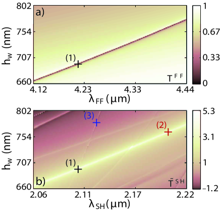
Figure 7: Spectra of transmission coefficient for the cylindrical texture determined for different waveguide heights under normal incidence. a) Spectra at the fundamental wavelength. b) Spectra at SH wavelengths (logarithmic scale).

The spectrum of radiated SH in the direction of the incoming wave, presented in Fig. 7(b), exhibits distinct maxima along the dispersion curves of the inherited and intrinsic resonances. For example, for the inherited $\mathrm{TE}_{0}$-resonance at $\lambda_{SH}=$ $2.126\text{\,}\mathrm{\SIUnitSymbolMicro m}$ and $0pt_{w}=$ $780\text{\,}\mathrm{nm}$ (blue cross (3)) the SHG enhancement as compared to a uniform GaAs layer with the same volume is $T^{SH}=10^{0.77}\approx 5.9$. The inherited resonance at $\lambda_{SH}=$ $2.201\text{\,}\mathrm{\SIUnitSymbolMicro m}$ and $0pt_{w}=$ $763\text{\,}\mathrm{nm}$ (red cross (2)) yields $T^{SH}=10^{3.95}$.

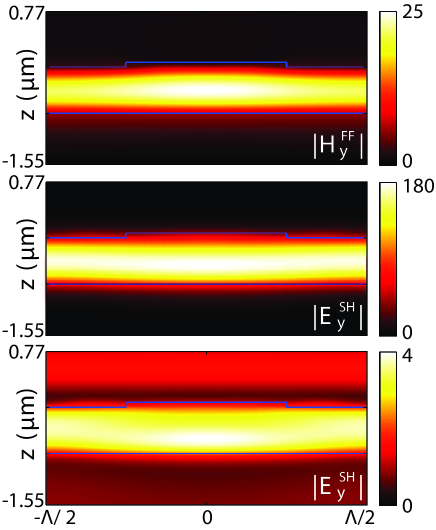
Figure 8: Magnetic and electric field distributions at simultaneous resonance wavelength $\lambda_{FF}=$ $4.213\text{\,}\mathrm{\SIUnitSymbolMicro m}$ and $h_{w}=$ $696\text{\,}\mathrm{nm}$. a) $|H_{y}^{FF}|$ of the fundamental $\mathrm{TM}_{0}$-resonance at the FF. b) $|E_{y}^{SH}|$ of simultaneous resonance at SH. c) $|E_{y}^{SH}|$ of intrinsic $\mathrm{TE}_{0}$ mode at SH wavelength $\lambda_{SH}=\lambda_{FF}/2=$ $2.107\text{\,}\mathrm{\SIUnitSymbolMicro m}$ for TM polarized incident plane wave.

We have designed a 2D periodic device in which inherited and intrinsic resonances can be simultaneously excited, the corresponding parameters being $\lambda_{FF}=$ $4.213\text{\,}\mathrm{\SIUnitSymbolMicro m}$ and $0pt_{w}=$ $696\text{\,}\mathrm{nm}$ (black cross (1)). This double resonance leads to an intensity enhancement of $I^{SH}\approx 10^{5}$ as compared to the reference uniform layer. The spatial profile of the magnetic field, calculated in the $x\vbox{ \hrule width=3.33333pt,height=0.0pt}z$-plane passing through the center of the cylinder ($y=0$) is displayed in Fig. 8(a). The field distribution closely resembles the profile of the $\mathrm{TM}_{0}$-mode, showing strong field enhancement and increased field confined in the waveguide as compared to the 1D-case. Our simulations suggest that normal incidence and a larger waveguide thickness favor stronger confinement. Moreover, the intrinsic $\mathrm{TE}_{0}$ mode profile is given in Fig. 8(c). As in the 1D-case, it strongly influences the shape of the SH-field inside the textured waveguide, as per Fig. 8(b).

V Conclusion

We have presented an extension of the generalized source method to analyze SHG in 2D periodic structures containing non-centrosymmetric, quadratically nonlinear optical materials. The linear and nonlinear parts of the calculations are decoupled in the undepleted pump approximation and a three-step computational process was derived. We introduced the correct Fourier-factorization rule for inhomogeneous problems and its beneficial effect on the convergence in the nonlinear calculations was clearly shown. In a benchmark structure the asymptotic runtime estimate of ${\mathcal{O}}(N\log(N)N_{l}\log(N_{l}))$ was validated, which renders the GSM especially suitable for modeling low permittivity contrast, dielectric gratings.

As a practical application we optimized the design of 1D and 2D textured GaAs slab waveguides to achieve maximal radiated SH by simultaneous excitation of linear and nonlinear slab waveguide modes. In a addition to an analytical estimate for the resonance frequencies of the textured slab waveguide, investigation of the field profiles allowed us to identify the nature of the resonances responsible for the remarkably high intensity enhancement of more than $8$ orders of magnitude in comparison to the SH radiated by a uniform slab. Importantly, the formalism presented in this study can be extended to several other key nonlinear optical processes, including surface SHG from centrosymmetric materials and higher-harmonic generation. Our method can be further extended beyond the undepleted pump approximation by allowing a self-consistent coupling between the FF and SH optical waves. In a similar manner, Kerr-nonlinear optical materials can be considered as well, a topic that we plan to address in a future study.

- (1) N. Bloembergen and P. S. Pershan, “Light waves at boundary of nonlinear media,” Phys. Rev. 128, 606–622 (1962).
- (2) P. S. Pershan, “Nonlinear optical properties of solids: energy considerations,” Phys. Rev. 130, 919–929 (1963).
- (3) W. Fan, S. Zhang, N. C. Panoiu, A. Abdenour, S. Krishna, R. M. Osgood, K. J. Malloy, and S. R. J. Brueck, “Second harmonic generation from a nanopatterned isotropic nonlinear material,” Nano Lett. 6, 1027–1030 (2006).
- (4) M. W. Klein, C. Enkrich, M. Wegener, and S. Linden, “Second-harmonic generation from magnetic meta-materials,” Science 313, 502–504 (2006).
- (5) J. A. H. van Nieuwstadt, M. Sandtke, R. H. Harmsen, F. B. Segerink, J. C. Prangsma, S. Enoch, and L. Kuipers, “Strong modification of the nonlinear optical response of metallic subwavelength hole arrays,” Phys. Rev. Lett. 97, 146102 (2006).
- (6) V. K. Valev, A. V. Silhanek, N. Verellen, W. Gillijns, P. Van Dorpe, O. A. Aktsipetrov, G. A. E. Vandenbosch, V. V. Moshchalkov, and T. Verbiest, “Asymmetric optical second-harmonic generation from chiral G-shaped gold nanostructures,” Phys. Rev. Lett. 104, 127401 (2010).
- (7) V. K. Valev, J. J. Baumberg, B. De Clercq, N. Braz, X. Zheng, E. J. Osley, S. Vandendriessche, M. Hojeij, C. Blejean, J. Mertens, C. G. Biris, V. Volskiy, M. Ameloot, Y. Ekinci, G. A. E. Vandenbosch, P. A. Warburton, V. V. Moshchalkov, N. C. Panoiu, and T. Verbiest, “Nonlinear superchiral meta-surfaces: tuning chirality and disentangling non-reciprocity at the nanoscale,” Adv. Mater. 26, 4074–4081 (2014).
- (8) K. Chen, C. Durak, J. R. Heflin, and H. D. Robinson, “Plasmon-enhanced second-harmonic generation from ionic self-assembled multilayer films,” Nano Lett. 7, 254–258 (2007).
- (9) J. Lee, M. Tymchenko, C. Argyropoulos, P.-Y. Chen, F. Lu, F. Demmerle, G. Boehm, M. C. Amann, A. Alu, and M. A. Belkin, “Giant nonlinear response from plasmonic metasurfaces coupled to intersubband transitions,” Nature 511, 65–69 (2014).
- (10) M. G. Moharam, E. B. Grann, D. A. Pommet, and T. K. Gaylord, “Formulation for stable and efficient implementation of the rigorous coupled-wave analysis of binary gratings,” J. Opt. Soc. Am. A. 12, 1068–1076 (1995).
- (11) L. Li, “New formulation of the Fourier modal method for crossed surface-relief gratings,” J. Opt. Soc. Am. A. 14, 2758–2767 (1997).
- (12) P. Lalanne and G. M. Morris, “Highly improved convergence of the coupled-wave method for TM polarization,” J. Opt. Soc. Am. A. 13, 779–784 (1996).
- (13) T. Schuster, J. Ruoff, N. Kerwien, S. Rafler, and W. Osten, “Normal vector method for convergence improvement using the RCWA for crossed gratings,” J. Opt. Soc. Am. A. 24, 2880–2890 (2007).
- (14) Photon Design Ltd., “OmniSim/RCWA,” http://www.photond.com/products/omnisim.htm
- (15) S. Essig and K. Busch, “Generation of adaptive coordinates and their use in the Fourier Modal Method,” Opt. Express 18, 23258–23274 (2010).
- (16) J. Chandezon, G. Raoult, and D. Maystre, “A new theoretical method for diffraction gratings and its numerical application,” J. Opt. 11, 235–241 (1980).
- (17) L. Li, J. Chandezon, G. Granet, and J.-P. Plumey “Rigorous and efficient grating-analysis method made easy for optical engineers,” Appl. Opt. 38, 304–313 (1999).
- (18) J. E. Sipe, “New Green-function formalism for surface optics,” J. Opt. Soc. Am. B. 4, 481–489 (1987).
- (19) T. Magath and A. E. Serebryannikov, “Fast iterative, coupled-integral-equation technique for inhomogeneous profiled and periodic slabs,” J. Opt. Soc. Am. A. 22, 2405–2418 (2005).
- (20) A. A. Shcherbakov and A. V. Tishchenko, “New fast and memory-sparing method for rigorous electromagnetic analysis of 2D periodic dielectric structures,” J. Quant. Spectrosc. Radiat. Transfer 113, 158–171 (2012).
- (21) E. Popov and M. Neviere, “Surface-enhanced second-harmonic generation in nonlinear corrugated dielectrics: new theoretical approaches,” J. Opt. Soc. Am. B. 11, 1555–1564 (1994).
- (22) W. Nakagawa, R.-C. Tyan, and Y. Fainman, “Analysis of enhanced second-harmonic generation in periodic nanostructures using modified rigorous coupled-wave analysis in the undepleted-pump approximation,” J. Opt. Soc. Am. A. 19, 1919–1928 (2002).
- (23) B. Bai and J. Turunen, “Fourier modal method for the analysis of second-harmonic generation in two-dimensionally periodic structures containing anisotropic materials,” J. Opt. Soc. Am. B. 24, 1105–1112 (2007).
- (24) T. Paul, C. Rockstuhl, and F. Lederer, “A numerical approach for analyzing higher harmonic generation in multilayer nanostructures,” J. Opt. Soc. Am. B. 27, 1118–1130 (2010).
- (25) T.-W. Lee and S. C. Hagness, “Pseudospectral time-domain methods for modeling optical wave propagation in second-order nonlinear materials,” J. Opt. Soc. Am. B. 21, 330–342 (2004).
- (26) C. M. Reinke, A. Jafarpour, B. Momeni, M. Soltani, S. Khorasani, A. Adibi, Y. Xu, and R. Lee “Nonlinear finite-difference time-domain method for the simulation of anisotropic, , and optical effects,” IEEE J. Lightwave Technol. 24, 624–634 (2006).
- (27) A. R. Cowan and J. F. Young, “Mode matching for second-harmonic generation in photonic crystal waveguides,” Phys. Rev. B 65, 085106 (2002).
- (28) C. G. Biris and N. C. Panoiu, “Second harmonic generation in metamaterials based on homogeneous centrosymmetric nanowires,” Phys. Rev. B 81, 195102 (2010).
- (29) J. Xu and X. Zhang, “Second harmonic generation in three-dimensional structures based on homogeneous centrosymmetric metallic spheres,” Opt. Express 20, 1668–1684 (2012).
- (30) R. E. Blahut, Fast algorithms for digital signal processing (Addison–Wesley, 1985).
- (31) A. A. Shcherbakov and A. V. Tishchenko, “Fast numerical method for modelling one-dimensional diffraction gratings,” Quantum. Electron. 40, 538–544 (2010).
- (32) L. Li, “Use of Fourier series in the analysis of discontinuous periodic structures,” J. Opt. Soc. Am. A. 13, 1870–1876 (1996).
- (33) M. Weismann, D. F. G. Gallagher, and N. C. Panoiu, “Generalized source method for modeling nonlinear diffraction in planar periodic structures,” Proc. SPIE 9131, 913115 (2014).
- (34) A. A. Shcherbakov and A. V. Tishchenko, “Efficient curvilinear coordinate method for grating diffraction simulation,” Opt. Express 21, 25236–25247 (2013).
- (35) R. W. Boyd, Nonlinear Optics (Academic Press, 2008).
- (36) N. C. Panoiu and R. M. Osgood “Enhanced optical absorption for photovoltaics via excitation of waveguide and plasmon-polariton modes,” Opt. Lett. 32, 2825–2827 (2007).
- (37) C. G. Biris and N. C. Panoiu, “Excitation of dark plasmonic cavity modes via nonlinearly induced dipoles: applications to near-infrared plasmonic sensing,” Nanotechnol. 22, 235502 (2011).