Quasiclassical theory of quantum defect
and spectrum of highly excited rubidium atoms

Abstract

We report on a significant discrepancy between recently published highly accurate variational calculations and precise measurements of the spectrum of Rydberg states in ⁸⁷Rb on the energy scale of fine splitting. Introducing a modified effective single-electron potential we determine the spectrum of the outermost bound electron from a standard WKB approach. Overall very good agreement with precise spectroscopic data is obtained.

I Introduction

The spectrum of the outermost bound electron of an alkali atom like ⁸⁷Rb is hydrogen like, but lacks the $n^{2}$-degeneracy of the eigenstates labeled by the principal quantum number $n$ of the pure Coulomb potential Gallagher (1994),We use scaled variables so that length is measured in units of the Bohr radius $a_{B}=\frac{\hslash^{2}}{m_{e}}\frac{4\pi\varepsilon_{0}}{\left|e\right|^{2}}\simeq$5.2918\text{\times}{10}^{-11}\text{\,}\mathrm{m}$$ and energy is measured in units of Rydberg, $\text{Ry}=\frac{m_{e}\left|e\right|^{4}}{8\varepsilon_{0}^{2}h^{2}}\simeq$13.605\text{\,}\mathrm{eV}$$.

$$E_{n,l}=-\frac{1}{\left(n-\delta_{l}\right)^{2}}.$$ (1)

This effect is the well-known quantum defect $\delta_{l}$, resulting from the interaction of the outermost electron with the ionic core of the atom and the nucleus. In a refined version of the statistical Thomas-Fermi theory Goeppert Mayer (1941), an effective potential determining the interaction between the outermost electron and the nucleus can accurately be modeled by a spherically symmetric potential $V_{\mathrm{eff}}\left(r;l\right)$ depending on the distance $r$ from the center and depending on the orbital angular momentum $l\in\left\{0,1,2,\ldots,n-1\right\}$ Greene and Aymar (1991); Marinescu et al. (1994),We use scaled variables so that length is measured in units of the Bohr radius $a_{B}=\frac{\hslash^{2}}{m_{e}}\frac{4\pi\varepsilon_{0}}{\left|e\right|^{2}}\simeq$5.2918\text{\times}{10}^{-11}\text{\,}\mathrm{m}$$ and energy is measured in units of Rydberg, $\text{Ry}=\frac{m_{e}\left|e\right|^{4}}{8\varepsilon_{0}^{2}h^{2}}\simeq$13.605\text{\,}\mathrm{eV}$$. :

$$V_{\mathrm{eff}}\left(r;l\right)=-2\left[\frac{Z_{\mathrm{eff}}\left(r;l\right)}{r}+V_{\mathrm{pol}}\left(r;l\right)\right]$$ (2)

Here the function $Z_{\mathrm{eff}}\left(r;l\right)$ represents a position-dependent weight function that interpolates the value of the charge between unity for large $r$ and charge number $Z$ near to the nucleus for $r\rightarrow 0$, and $V_{\mathrm{pol}}\left(r;l\right)$ represents a short-ranged interaction taking into account the static electric polarizability of the ionic core Born (1925); Gallagher (1994).

Overall good agreement with spectroscopic data of alkali atoms (but discarding the fine splitting) has been reported in Marinescu et al. (1994) choosing

$$Z_{\mathrm{eff}}\left(r;l\right)=1+(Z-1)e^{-ra_{1}\left(l\right)}-re^{-ra_{2}\left(l\right)}\left[a_{3}\left(l\right)+ra_{4}\left(l\right)\right]$$ (3)

and

$$V_{\mathrm{pol}}\left(r;l\right)=\frac{\alpha_{c}}{2}\frac{1-\exp\left[-\left(\frac{r}{r_{c}\left(l\right)}\right)^{6}\right]}{r^{4}}.$$ (4)

A table of the parameters $a_{1}(l)$, $a_{2}(l)$, $a_{3}(l)$, $a_{4}(l)$, $\alpha_{c}$, and $r_{c}\left(l\right)$ can be found in Marinescu et al. (1994).

In an attempt to also describe the fine splitting of the excitation spectrum of the outermost electron of ⁸⁷Rb, it has been suggested Greene and Aymar (1991) to superimpose a posteriori a spin-orbit term

$$\widetilde{V}_{\mathrm{SO}}\left(r;j,l\right)=\frac{V_{\mathrm{SO}}\left(r;j,l\right)}{\left[1-\alpha^{2}V_{\mathrm{eff}}\left(r;l\right)\right]^{2}},$$ (5)

on the potential $V_{\mathrm{eff}}\left(r;l\right)$, which then influences the spectrum $E_{n,j,l}$ on the scale of fine splitting and the orbitals $\psi_{n,j,l}(r)$ accessible to the outermost electron. Here

$$V_{\mathrm{SO}}\left(r;j,l\right)=\alpha^{2}\frac{1}{r}\frac{\partial V_{\mathrm{eff}}\left(r;l\right)}{\partial r}g\left(j,l\right),$$ (6)

and $\alpha=\frac{\lambda_{C}}{a_{B}}\simeq\frac{1}{137.036}$ denotes the fine-structure constant, and

$$g\left(j,l\right)=\begin{cases}0&\text{ if }l=0,\\ \\ \frac{j\left(j+1\right)-l\left(l+1\right)-\frac{3}{4}}{2}&\text{ if }l\geq 1,\end{cases}$$ (7)

where $j\in\left\{l-\frac{1}{2},l+\frac{1}{2}\right\}$. To determine those orbitals (with principal quantum number $n=n_{r}+l+1$ and radial quantum number $n_{r}\in\mathbb{N}_{0}$), a normalizable solution to the Schrödinger eigenvalue problem for the radial wavefunction $U_{n,j,l}(r)=rR_{n,j,l}\left(r\right)$ and associated eigenvalues $E_{n,j,l}<0$ is required:

$$\left[-\frac{d^{2}}{dr^{2}}+\frac{l(l+1)}{r^{2}}+\widetilde{V}\left(r;j,l\right)-E_{n,j,l}\right]U_{n,j,l}(r)=0,$$ (8)

where

$$\widetilde{V}\left(r;j,l\right)=V_{\mathrm{eff}}\left(r;l\right)+\widetilde{V}_{\mathrm{SO}}\left(r;j,l\right)$$ (9)

denotes the effective single-electron potential.

A highly accurate variational calculation of the excitation spectrum of the outermost electron of ⁸⁷Rb has been carried out recently Pawlak et al. (2014), in which the authors expand the radial wavefunction of the Schrödinger eigenvalue problem (8) in a basis spanned by $500$ Slater-type orbitals (STOs). On the other hand, modern high precision spectroscopy of Rydberg levels of ⁸⁷Rb has been conducted recently. Millimeter-wave spectroscopy employing selective field ionization allows for precise measurements of the energy differences between Rydberg levels Li et al. (2003). An independent approach is to perform purely optical measurements on absolute Rydberg level energies by observing electromagnetically induced transparency (EIT) Mohapatra et al. (2007); Mack et al. (2011). However, there is a systematic discrepancy between variational calculations and the spectroscopic measurements of the fine splitting

$$\Delta E_{n,l}=E_{n,l-\frac{1}{2},l}-E_{n,l+\frac{1}{2},l}$$ (10)

as shown in Tables 1 and 2. Given the fact that the error bars of the independent experiments Li et al. (2003); Mack et al. (2011) are below $1.1\text{\,}\mathrm{MHz}$ down to $20\text{\,}\mathrm{kHz}$, and on the other hand considering the high accuracy of the numerical calculations presented in Pawlak et al. (2014), such a discrepancy between experiment and theory is indeed significant.

Table 1: Fine splitting $\Delta E_{n,l=1}$ for P states in [$\mathrm{MHz}$].

State $\left|n,l=1\right\rangle$	Exp. Sansonetti (2006)	Exp. Li et al. (2003)	Theory Pawlak et al. (2014)	Theory (this work)
8P	$565.1(4)\times 10^{3}$	N/A	$602.00\times 10^{3}$	$567.75\times 10^{3}$
10P	$219.1(4)\times 10^{3}$	N/A	$231.87\times 10^{3}$	$218.77\times 10^{3}$
30P	N/A	$4246.30(5)$	$4500.50$	$4246.46$
35P	N/A	$2566.41(32)$	$2717.41$	$2566.28$
45P	N/A	$1144.09(13)$	$1217.24$	$1143.95$
55P	N/A	$605.77(7)$	$644.81$	$605.68$
60P	N/A	$460.76(5)$	$480.32$	$460.68$

Table 2: Fine splitting $\Delta E_{n,l=2}$ for D states in [$\mathrm{MHz}$].

State $\left|n,l=2\right\rangle$	Exp. Sansonetti (2006)	Exp. Li et al. (2003)	Exp. Mack et al. (2011)	Theory Pawlak et al. (2014)	Theory (this work)
8D	$30.4(4)\times 10^{3}$	N/A	N/A	$113.17\times 10^{3}$	$36.42\times 10^{3}$
10D	$14.9(2)\times 10^{3}$	N/A	N/A	$52.05\times 10^{3}$	$16.56\times 10^{3}$
30D	N/A	$452.42(18)$	$452.5(11)$	$1447.53$	$456.13$
35D	N/A	$279.65(10)$	$280.4(11)$	$894.84$	$281.52$
45D	N/A	$128.33(4)$	$127.8(11)$	$407.64$	$128.98$
55D	N/A	$69.17(2)$	$69.4(11)$	$223.71$	$69.47$
57D	N/A	$61.98(2)$	$62.2(11)$	$197.39$	$62.24$

So, what could be the reason for the reported discrepancies? First, it should be pointed out that in the variational calculations Pawlak et al. (2014) a slightly different potential was used, that is,

$$V\left(r;j,l\right)=V_{\mathrm{eff}}\left(r;l\right)+V_{\mathrm{SO}}\left(r;j,l\right).$$ (11)

Certainly, within the first-order perturbation theory there exists no noticeable discrepancy in the spectrum of the outermost electron on the fine-splitting scale, when taking into account the spin-orbit forces with $V_{\mathrm{SO}}\left(r;j,l\right)$ instead of working with $\widetilde{V}_{\mathrm{SO}}\left(r;j,l\right)$. This is due to the differences being negligible for $r>Z\alpha^{2}$. However, since $V_{\mathrm{SO}}\left(r;j,l\right)$ eventually dominates even the contribution of the centrifugal barrier term $\frac{l\left(l+1\right)}{r^{2}}$ within the tiny region $0<r\lesssim\alpha^{2}Z$, a subtle problem with a non-normalizable radial wavefunction $U_{n,j,l}(r)$ emerges when attempting to solve the Schrödinger eigenvalue problem for any $l>0$ with the potential $V_{\mathrm{SO}}\left(r;j,l\right)$. Such a problem is absent when one works with $\widetilde{V}_{\mathrm{SO}}\left(r;j,l\right)$ Greene and Aymar (1991).

A variational calculation with the potential (11) employing $N=500$ normalizable STOs as basis functions thus engenders a systematic (small) error of the matrix elements calculated in Pawlak et al. (2014) on the fine-splitting scale. When employing substantially more STOs this error would certainly become larger. With $N=500$ STOs the discrepancy of these theoretical results with the high precision spectroscopic data, as shown in Tables 1 and 2, is far too large to be corrected by simply replacing $V_{\mathrm{SO}}\left(r;j,l\right)$ with $\widetilde{V}_{\mathrm{SO}}\left(r;j,l\right)$. Hence another explanation is required.

II Quasiclassical approach and fine splitting of the highly excited ⁸⁷Rb

In 1941 alkali atoms have already been studied in the context of modern quantum mechanics in the seminal work by Goeppert Mayer Goeppert Mayer (1941), who emphasized the exceptional role of the $l=1$ and $l=2$ orbitals. According to Goeppert Mayer, the outermost electron of an alkali atom is governed by an effective $r$-dependent charge term

$$Z_{\mathrm{eff}}\left(r\right)=1+(Z-1)F(r),$$ (12)

where the function $F(r)$ has been determined by employing the semi-classical statistical Thomas-Fermi approach to the many-electron-atom problem, posing the boundary conditions as $\lim_{r\rightarrow 0}F(r)=1$ and $\lim_{r\rightarrow\infty}F\left(r\right)=0$. As discussed by Schwinger Schwinger (2001), this approach ceases to be valid in the inner shell region $Z^{-1}<r<Z^{-\frac{1}{3}}$ of the atom. Therefore, taking into account the fine splitting in the spectrum of the outermost electron of alkali atoms a posteriori by simply adding the phenomenological spin-orbit term (5) to (2), resulting in the effective single-electron potential (9), seems to be questionable on general grounds in that inner shell region.

On a more fundamental level, the treatment of relativistic effects in multi-electron-atom spectra requires an a priori microscopic description based on the well-known Breit-Pauli Hamiltonian Bethe and Salpeter (1957); Froese-Fischer et al. (1997)

$$\mathscr{H}=\mathscr{H}_{\mathrm{nr}}+\mathscr{H}_{\mathrm{rs}}+\mathscr{H}_{\mathrm{fs}}.$$ (13)

Here $\mathscr{H}_{\mathrm{nr}}$ is the ordinary nonrelativistic many-electron Hamiltonian, while the relativistic corrections are represented by the perturbation operators $\mathscr{H}_{\mathrm{rs}}$ and $\mathscr{H}_{\mathrm{fs}}$. The perturbation term $\mathscr{H}_{\mathrm{rs}}$ contains all the relativistic perturbations like mass correction, one- and two-body Darwin terms, and further the spin-spin contact and orbit-orbit terms, which all commute with the total angular momentum $\mathbf{L}$ and total spin $\mathbf{S}$, thus effectuating only small shifts of the spectrum of the nonrelativistic Hamiltonian $\mathscr{H}_{\mathrm{nr}}$. The perturbation operator $\mathscr{H}_{\mathrm{fs}}$ on the other hand breaks the rotational symmetry. It consists of the standard nuclear spin-orbit, the spin-other-orbit, and the spin-spin dipole interaction terms, which all commute with $\mathbf{J}=\mathbf{L}+\mathbf{S}$, but not with $\mathbf{L}$ or with $\mathbf{S}$ separately, thus inducing the fine splitting of the nonrelativistic spectrum.

Although the proposed functional form of the potential (11) is highly plausible on physical grounds outside the inner core region $r>Z^{-\frac{1}{3}}$, prima facie it appears to be inconsistent to lump the aforementioned relativistic many-body forces into an effective single-electron potential of the functional form (11), so that it provides an accurate description also for small distances $Z^{-1}<r<Z^{-\frac{1}{3}}$.

In the absence of a better microscopic theory for an effective single-electron potential $V_{\mathrm{eff}}\left(r;j,l\right)$ describing the fine splitting of the spectrum of the outermost electron in the alkali atoms, we introduce a cutoff at a distance $r_{\mathrm{so}}(l)$ with $Z^{-1}<r_{\mathrm{so}}(l)<Z^{-\frac{1}{3}}$ so that the effective single-electron potential is now described by the following modified potential:

$$\widetilde{V}_{\mathrm{mod}}\left(r;j,l\right)=\begin{cases}V_{\mathrm{eff}}\left(r;l\right)&\text{if }0\leq r\leq r_{\mathrm{so}}\left(l\right),\\ \\ V_{\mathrm{eff}}\left(r;l\right)+V_{\mathrm{SO}}\left(r;j,l\right)&\text{if }r>r_{\mathrm{so}}\left(l\right).\end{cases}$$ (14)

The choice We use scaled variables so that length is measured in units of the Bohr radius $a_{B}=\frac{\hslash^{2}}{m_{e}}\frac{4\pi\varepsilon_{0}}{\left|e\right|^{2}}\simeq$5.2918\text{\times}{10}^{-11}\text{\,}\mathrm{m}$$ and energy is measured in units of Rydberg, $\text{Ry}=\frac{m_{e}\left|e\right|^{4}}{8\varepsilon_{0}^{2}h^{2}}\simeq$13.605\text{\,}\mathrm{eV}$$.

$$r_{\mathrm{so}}\left(l=1\right)=0.029483\times r_{c}\left(l=1\right)=0.0442825,$$

$$r_{\mathrm{so}}\left(l=2\right)=0.051262\times r_{c}\left(l=2\right)=0.2495720,$$

gives a surprisingly accurate description of the fine splitting in the spectroscopic data for all principal quantum numbers $n$, see Tables 1 and 2.

The calculation of the spectrum of the outermost bound electron is then reduced to solving the radial Schrödinger equation (8) with the modified potential $\widetilde{V}_{\mathrm{mod}}\left(r;j,l\right)$. The resulting spectrum is actually hydrogen like, that is,

$$E_{n,j,l}=-\frac{1}{\left(n-\Delta_{j,l}\right)^{2}},$$ (16)

where $\Delta_{j,l}$ denotes a quantum defect comprising also the fine splitting. In actual fact the quantum defect describes a reduction of the number of nodes $n_{r}$ of the radial wavefunction for $l=0,1,2$ as a result of the short-range interaction of the outermost electron with the ionic core of the atom. Because the higher the orbital angular momentum quantum number $l$, the lower the probability of the electron being located near to the center, it is clear that the quantum defect decreases rapidly with increasing orbital angular momentum $l$. Therefore, $\Delta_{j,l}$ is only notably different from zero for $l=0,1,2$.

Writing $\Delta_{j,l}=\delta_{l}+\eta_{j,l}$ with $\eta_{j,l}\ll\delta_{l}$, the fine splitting to leading order in $\alpha^{2}$ is:

$$\Delta E_{n,l}=2\frac{\eta_{l-\frac{1}{2},l}-\eta_{l+\frac{1}{2},l}}{\left(n-\delta_{l}\right)^{3}}$$ (17)

The quasiclassical momentum $p\equiv\sqrt{-Q}$ of the bound electron with orbital angular momentum $l>0$, total angular momentum $j=l\pm\frac{1}{2}$, and taking into account the Langer shift $l(l+1)\rightarrow\left(l+\frac{1}{2}\right)^{2}$ in the centrifugal barrier Langer (1937); Berry and Mount (1972), is then given by

$$Q\left(r;j,l,E\right)=\frac{\left(l+\frac{1}{2}\right)^{2}}{r^{2}}+\widetilde{V}_{\mathrm{mod}}\left(r;j,l\right)-E.$$ (18)

For $l=0$ the centrifugal barrier term and the spin-orbit potential are absent.

Considering high excitation energies $E<0$ of the bound outermost electron, i.e. a principal quantum number $n\gg 1$, the respective positions of the turning points $r^{\left(\pm\right)}$ are given approximately by

$$r^{\left(-\right)} =\frac{\left(l+\frac{1}{2}\right)^{2}}{1+\sqrt{1+\left(l+\frac{1}{2}\right)^{2}E}} \text{if }l\geq 3,$$

$$r^{\left(+\right)} \simeq\frac{1}{-E}\left[1+\sqrt{1+\left(l+\frac{1}{2}\right)^{2}E}\right] \text{if }l\geq 1,$$

where $0<l\ll\frac{1}{\sqrt{-E}}$. Of course for $l=0$ only a single (large) turning point $r^{\left(+\right)}=\frac{2}{-E}$ exists due to the absence of the centrifugal barrier. However, the lower turning points $r^{\left(-\right)}$ are strongly modified for $l=1,2$ compared to the pure Coulomb potential case taking into account the core polarization. For $l=1,2$ the relation $r^{\left(-\right)}\left(l\right)\simeq 0.02\times r_{c}\left(l\right)$ holds; that is, $r^{\left(-\right)}\left(l=1\right)\simeq 0.03472$ and $r^{\left(-\right)}\left(l=2\right)\simeq 0.12827$ We use scaled variables so that length is measured in units of the Bohr radius $a_{B}=\frac{\hslash^{2}}{m_{e}}\frac{4\pi\varepsilon_{0}}{\left|e\right|^{2}}\simeq$5.2918\text{\times}{10}^{-11}\text{\,}\mathrm{m}$$ and energy is measured in units of Rydberg, $\text{Ry}=\frac{m_{e}\left|e\right|^{4}}{8\varepsilon_{0}^{2}h^{2}}\simeq$13.605\text{\,}\mathrm{eV}$$. . Since the cutoff $r_{\mathrm{so}}\left(l\right)$ in (II) is substantially above those values of the lower turning points $r^{\left(-\right)}\left(l\right)$, a quasiclassical calculation of the fine-split spectrum of the bound outermost electron is reliable.

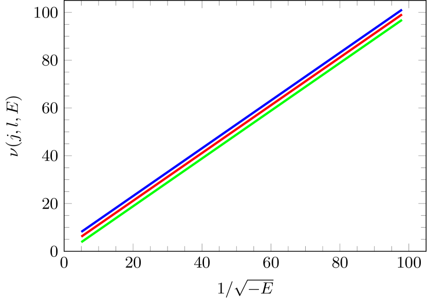
Figure 1: (Color online) The action integral $\nu\left(j,l,E\right)$ associated with the effective single-electron potential $\widetilde{V}_{\mathrm{mod}}\left(r;j,l\right)$ vs. scaled energy $\frac{1}{\sqrt{-E}}$ for $l=0$ (blue line), $l=1$ (red line), $l=2$ (green line), all for $j=l+\frac{1}{2}$. The curves for $j=l-\frac{1}{2}$ only differ by a tiny shift proportional to $\alpha^{2}$.

For a chosen radial quantum number $n_{r}$, the associated eigenvalues $E=E_{n,j,l}<0$ of the outermost electron now follow from the WKB patching condition Migdal (1977); Karnakov and Krainov (2013):

$$\nu\left(j,l,E\right)\overset{!}{=}\begin{cases}n_{r}+1&\text{if }l=0,\\ \\ n_{r}+\frac{1}{2}&\text{if }l>0,\end{cases}$$ (20)

where $\nu\left(j,l,E\right)$ denotes the action integral

$$\nu\left(j,l,E\right) =\frac{1}{\pi}\int_{r^{\left(-\right)}}^{r^{\left(+\right)}}\mathrm{d}r\sqrt{-Q\left(r;j,l,E\right)}$$

$$=\frac{1}{2\pi}\oint\mathrm{d}r\,p\left(r;j,l,E\right).$$ (21)

Plotting the function $\nu\left(j,l,E\right)$ versus $\frac{1}{\sqrt{-E}}$ for $l=0,1,2$ clearly reveals a linear dependence of the form $\nu\left(j,l,E\right)=\frac{1}{\sqrt{-E}}+c\left(j,l\right)$, see Fig. 1.

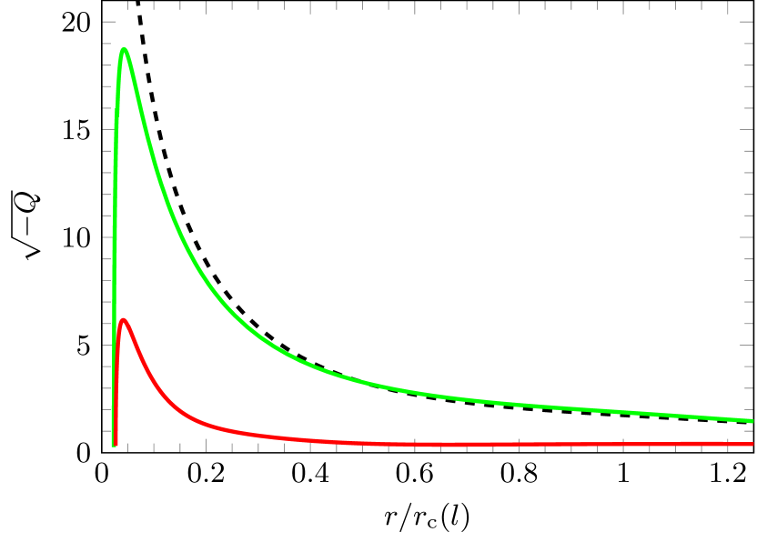
Figure 2: (Color online) The quasiclassical momentum $\sqrt{-Q\left(r;j,l,E\right)}$ vs. scaled distance $\frac{r}{r_{c}\left(l\right)}$ for $l=0$ (dashed black), $l=1$ (green), $l=2$ (red), for $E=E_{n,j,l}$ corresponding to principal quantum number $n=57$ and $j=l+\frac{1}{2}$. The main contribution to the quantum defect values in (24) originates from the inner core region $r<r_{c}\left(l\right)$.

Table 3: The values of quantum defect $\Delta_{j,l}$ associated with the Rydberg level $n=57$ for $l=0,1,2$.

Quantum defect $\Delta_{j,l}$	Exp. Li et al. (2003)	Exp. Mack et al. (2011)	Theory Pawlak et al. (2014)	Theory (this work)
$\Delta_{\nicefrac{{1}}{{2}},0}$	$3.1312419(10)$	$3.13125(2)$	$3.12791$	$3.13095$
$\Delta_{\nicefrac{{1}}{{2}},1}$	$2.6549831(10)$	N/A	$2.65795$	$2.65197$
$\Delta_{\nicefrac{{3}}{{2}},1}$	$2.6417735(10)$	N/A	$2.64399$	$2.63876$
$\Delta_{\nicefrac{{1}}{{2}},1}-\Delta_{\nicefrac{{3}}{{2}},1}$	$0.0132096(14)$	N/A	$0.01396$	$0.01321$
$\Delta_{\nicefrac{{3}}{{2}},2}$	$1.3478971(4)$	$1.34789(2)$	$1.35145$	$1.34851$
$\Delta_{\nicefrac{{5}}{{2}},2}$	$1.3462733(3)$	$1.34626(2)$	$1.34628$	$1.34688$
$\Delta_{\nicefrac{{3}}{{2}},2}-\Delta_{\nicefrac{{5}}{{2}},2}$	$0.0016238(5)$	$0.00163(3)$	$0.00517$	$0.00163$

According to Born (1925), for $A,B,C,D\in\mathbb{R}$, with $A>0$, $B>0$, $C>0$, and $\left|D\right|\ll C$ the following equality holds:

$$\frac{1}{2\pi}\oint\mathrm{d}r\sqrt{-A+\frac{2B}{r}-\frac{C}{r^{2}}+\frac{D}{r^{3}}}=\frac{B}{\sqrt{A}}-\sqrt{C}+\frac{BD}{2C\sqrt{C}}$$ (22)

For a pure Coulomb potential $A\equiv-E$, $B\equiv 1$, $C\equiv\left(l+\frac{1}{2}\right)^{2}$ and $D\equiv\alpha^{2}g\left(j,l\right)$. The corresponding action integral then reads

$$\nu^{\left(\mathrm{C}\right)}\left(j,l,E\right)=\begin{cases}\frac{1}{\sqrt{-E}}&\text{if }l=0,\\ \\ \frac{1}{\sqrt{-E}}-\left(l+\frac{1}{2}\right)+\frac{\alpha^{2}g\left(j,l\right)}{2\left(l+\frac{1}{2}\right)^{3}}&\text{if }l>0.\end{cases}$$ (23)

It is thus found from WKB theory that the quantum defect associated with the single-electron potential $\widetilde{V}_{\mathrm{mod}}\left(r;j,l\right)$ is:

$$\Delta_{j,l}=\lim_{E\rightarrow 0^{-}}\left[\nu\left(j,l,E\right)-\nu^{\left(\mathrm{C}\right)}\left(j,l,E\right)\right]$$ (24)

Ignoring spin-orbit coupling, i.e. for $\alpha=0$ , one has $\Delta_{j,l}\equiv\delta_{l}$, the standard quantum defect. For $l=0$ the centrifugal barrier and the spin-orbit coupling term (6) are zero, so $\Delta_{j,l}\rightarrow\Delta_{\frac{1}{2},0}\equiv\delta_{0}$.

The dependence of the quasiclassical momentum $\sqrt{-Q\left(r;j,l,E\right)}$ on the scaled distance $\frac{r}{r_{c}(l)}$ is shown for $l=0,1,2$ in Fig. 2. Clearly, it is the inner core region $r^{\left(-\right)}\left(l\right)<r<r_{c}(l)$ that provides the main contribution to the quantum defect values. We find, for $l=0,2$, that changing the fitting parameter $a_{3}\left(l\right)$ in (3) from its tabulated value in Marinescu et al. (1994) according to the scaling prescription $a_{3}\left(l=0\right)\rightarrow 0.814\times a_{3}\left(l=0\right)$ and $a_{3}\left(l=2\right)\rightarrow 0.914\times a_{3}\left(l=2\right)$, leads to a slight downward constant shift of the WKB-quantum defect. As a result of this change, the calculated WKB-quantum defect $\Delta_{l\pm\frac{1}{2},l}$ then agrees well with the spectroscopic data, see Table 3. Such a change of $a_{3}\left(l\right)$ does not affect the fine splitting values $\Delta E_{n,l}$ though. We also find that the dependence of the fine splitting $\Delta E_{n,l}$ on the principal quantum number $n$ is well described by (17) for all $n\geq 8$, see Tables 1 and 2.

In actual fact, for $r^{\left(+\right)}\gg r^{\left(-\right)}$, which is a criterion that is always met for high excitation energies $\sqrt{-E}\simeq 0$ of the outermost electron, the uniform Langer-WKB wavefunction $U_{n,j,l}^{\left(\mathrm{WKB}\right)}\left(r\right)$ Langer (1934); Bender and Orszag (1978), with $r^{\left(+\right)}$ considered as the only turning point, describes the numerical solution $U_{n,j,l}\left(r\right)$ to the radial differential equation (8) under the influence of the effective modified single-electron potential (14) rather accurately Sanayei and Schopohl . Only very near to the second turning point $r^{\left(-\right)}$, at a distance smaller than $r_{\mathrm{so}}\left(l\right)$, the Langer-WKB wavefunction $U_{n,j,l}^{\left(\mathrm{WKB}\right)}\left(r\right)$ ceases to be a good approximation to the numerical solution $U_{n,j,l}\left(r\right)$ of the radial Schrödinger equation (8) Sanayei and Schopohl .

III Conclusions

In this work we reported a significant discrepancy between experiment Li et al. (2003); Mack et al. (2011) and highly accurate variational calculations Pawlak et al. (2014) of the spectrum of Rydberg states of ⁸⁷Rb on the energy scale of the fine splitting. We discussed that the usual a posteriori adding of the relativistic spin-orbit potential to the effective single electron potential governing the outermost electron of alkali atoms is indeed inconsistent inside the inner atomic core region. In the absence of a full microscopic theory that lumps all many-body interactions together with the relativistic corrections into an effective single-electron potential in a consistent manner, we suggested a modified effective single-electron potential, see (14), that enables a correct description of the spectrum of Rydberg states on the fine splitting scale in terms of a simple WKB-action integral for all principal quantum numbers $n\geq 8$. Modern precision spectroscopy of highly excited Rydberg states thus enables the probing of the multi-electron correlation problem of the ionic core of alkali atoms. This is certainly a fascinating perspective for further experiments and theoretical studies.

*