k²U: A General Framework from $k$-Point Effective Schedulability Analysis to Utilization-Based Tests

Abstract

To deal with a large variety of workloads in different application domains in real-time embedded systems, a number of expressive task models have been developed. For each individual task model, researchers tend to develop different types of techniques for deriving schedulability tests with different computation complexity and performance. In this paper, we present a general schedulability analysis framework, namely the $\mathbf{k^{2}U}$ framework, that can be potentially applied to analyze a large set of real-time task models under any fixed-priority scheduling algorithm, on both uniprocessor and multiprocessor scheduling. The key to $\mathbf{k^{2}U}$ is a $k$-point effective schedulability test, which can be viewed as a “blackbox” interface. For any task model, if a corresponding $k$-point effective schedulability test can be constructed, then a sufficient utilization-based test can be automatically derived. We show the generality of $\mathbf{k^{2}U}$ by applying it to different task models, which results in new and improved tests compared to the state-of-the-art.

Analogously, a similar concept by testing only $k$ points with a different formulation has been studied by us in another framework, called $\mathbf{k^{2}Q}$, which provides quadratic bounds or utilization bounds based on a different formulation of schedulability test. With the quadratic and hyperbolic forms, $\mathbf{k^{2}Q}$ and $\mathbf{k^{2}U}$ frameworks can be used to provide many quantitive features to be measured, like the total utilization bounds, speed-up factors, etc., not only for uniprocessor scheduling but also for multiprocessor scheduling. These frameworks can be viewed as a “blackbox” interface for schedulability tests and response-time analysis.

1 Introduction

Given the emerging trend towards building complex cyber-physical systems that often integrate external and physical devices, many real-time and embedded systems are expected to handle a large variety of workloads. Different formal real-time task models have been developed to accurately represent these workloads with various characteristics. Examples include the sporadic task model [34], the multi-frame task model [35], the self-suspending task model [29], the directed-acyclic-graph (DAG) task model, etc. Many of such formal models have been shown to be expressive enough to accurately model real systems in practice. For example, the DAG task model has been used to represent many computation-parallel multimedia application systems and the self-suspending task model is suitable to model workloads that may interact with I/O devices. For each of these task models, researchers tend to develop different types of techniques that result in schedulability tests with different computation complexity and performance (e.g., different utilization bounds).

Over the years, real-time systems researchers have devoted a significant amount of time and efforts to efficiently analyze different task models. Many successful stories have been told. For many of the above-mentioned task models, efficient scheduling and schedulability analysis techniques have been developed (see [16] for a recent survey). Unfortunately, for certain complex models such as the self-suspending task model, existing schedulability tests are rather pessimistic, particularly for the multiprocessor case (e.g., no utilization-based schedulability test exists for globally-scheduled multiprocessor self-suspending task systems).

In this paper, we present $\mathbf{k^{2}U}$, a general schedulability analysis framework that is fundamentally based on a $k$-point effective schedulability test under fixed-priority scheduling. The key observation behind our proposed $k$-point test is the following. Traditional fixed-priority schedulability tests often have pseudo-polynomial-time (or even higher) complexity. For example, to verify the schedulability of a (constrained-deadline) task $\tau_{k}$ under fixed-priority scheduling in uniprocessor systems, the time-demand analysis (TDA) developed in [26] can be adopted. That is, if

$$\exists t\mbox{ with }0<t\leq D_{k}{\;\;and\;\;}C_{k}+\sum_{\tau_{i}\in hp(\tau_{k})}\left\lceil{\frac{t}{T_{i}}}\right\rceil C_{i}\leq t,$$ (1)

then task $\tau_{k}$ is schedulable under the fixed-priority scheduling algorithm, where $hp(\tau_{k})$ is the set of the tasks with higher priority than $\tau_{k}$, $D_{k}$, $C_{k}$, and $T_{i}$ represent $\tau_{k}$’s relative deadline, worst-case execution time, and period, respectively. TDA incurs pseudo-polynomial-time complexity to check the time points that lie in $(0,D_{k}]$ for Eq. (1).

To obtain sufficient schedulability tests under fixed priority scheduling with reduced time complexity (e.g., polynomial-time), our conceptual innovation is based on the observations by testing only a subset of such points to derive the minimum $C_{k}$ that cannot pass the schedulability tests. This idea is implemented in the $\mathbf{k^{2}U}$ framework by providing a general $k$-point effective schedulability test, which only needs to test $k$ points under any fixed-priority scheduling when checking schedulability of the task with the $k^{th}$ highest priority in the system. This $k$-point effective schedulability test can be viewed as a “blackbox” interface that can result in sufficient utilization-based tests. We show the generality of $\mathbf{k^{2}U}$ by applying it to analyze several concrete example task models, including the constrained- and arbitrary-deadline sporadic task models, the multi-frame task model, the self-suspending task model, and the DAG task model. Note that $\mathbf{k^{2}U}$ is not only applicable to uniprocessor systems, but also applicable to multiprocessor systems.

Related Work. An extensive amount of research has been conducted over the past forty years on verifying the schedulability of the classical sporadic task model in both uniprocessor and multiprocessor systems (see [16] for a survey of such results). Much progress has also been made in recent years on analyzing more complex task models that are more expressive. There have been several results in the literature with respect to utilization-based, e.g., [31, 22, 24, 37, 23, 7, 30], and non-utilization-based, e.g., [11, 20], schedulability tests for the sporadic real-time task model and its generalizations in uniprocessor systems. The approaches in [11, 20] convert the stair function $\left\lceil{\frac{t}{T_{i}}}\right\rceil$ in the time-demand analysis into a linear function if $t$ in Eq. (1) is large enough. The methods in [11, 20] are completely different from this paper, in which the linear function of task $\tau_{i}$ starts after $\frac{t}{T_{i}}\geq k$, in which our method is based on $k$ points, defined individually by $\tau_{1},\tau_{2},\ldots,\tau_{k}$.

Most of the existing utilization-based schedulability analyses focus on the total utilization bound. That is, if the total utilization of the task system is no more than the derived bound, the task system is schedulable by the scheduling policy. For example, the total utilization bounds derived in [31, 22, 10] are mainly for rate-monotonic (RM) scheduling, in which the results in [22] can be extended for arbitrary fixed-priority scheduling. Kuo et al. [23] further improve the total utilization bound by using the notion of divisibility. Lee et al. [24] use linear programming formulations for calculating total utilization bounds when the period of a task can be selected. Moreover, Wu et al. [37] adopt the Network Calculus to analyze the total utilization bounds of several task models.

The novelty of $\mathbf{k^{2}U}$ comes from a different perspective from these approaches [31, 22, 24, 37, 23]. We do not specifically seek for the total utilization bound. Instead, we look for the critical value in the specified sufficient schedulability test while verifying the schedulability of task $\tau_{k}$. A natural schedulability condition to express the schedulability of task $\tau_{k}$ is a hyperbolic bound, (to be shown in Lemma 1), whereas the corresponding total utilization bound can be obtained (in Lemmas 2 and 3).

The hyperbolic forms are the centric features in $\mathbf{k^{2}U}$ analysis, in which the test by Bini et al. [7] for sporadic real-time tasks and our recent result in [30] for bursty-interference analysis are both special cases and simple implications from the $\mathbf{k^{2}U}$ framework. With the hyperbolic forms, we are then able to provide many interesting observations with respect to the required quantitive features to be measured, like the total utilization bounds, speed-up factors, etc., not only for uniprocessor scheduling but also for multiprocessor scheduling. For more details, we will provide further explanations at the end of Sec. 4 after the framework is presented. For the studied task models to demonstrate the applicability of $\mathbf{k^{2}U}$, we will summarize some of the latest results on these task models in their corresponding sections.

Contributions. In this paper, we present a general schedulability analysis framework, $\mathbf{k^{2}U}$, that can be applied to analyze a number of complex real-time task models, on both uniprocessors and multiprocessors. For any task model, if a corresponding $k$-point effective schedulability test can be constructed, then a sufficient utilization-based test can be derived by the $\mathbf{k^{2}U}$ framework. We show the generality of $\mathbf{k^{2}U}$ by applying it to several task models, in which the results are better or more general compared to the state-of-the-art:

1. For uniprocessor constrained-deadline sporadic task systems, the speed-up factor of our obtained schedulability test is 1.76322. This value is the same as the lower bound and upper bound of deadline-monotonic (DM) scheduling shown by Davis et al. [18]. Our result is thus stronger (and requires a much simpler proof), as we show that the same factor holds for a polynomial-time schedulability test (not just the DM scheduler). For uniprocessor arbitrary-deadline sporadic task systems, our obtained utilization-based test works for any fixed-priority scheduling with arbitrary priority-ordering assignment.

2. For multiprocessor DAG task systems under global rate-monotonic (RM) scheduling, the capacity-augmentation factor, as defined in  [28] and Sec. 6 in this paper, of our obtained test is 3.62143. This result is better than the best existing result, which is 3.73, given by Li et al. [28]. Our result is also applicable for conditional sporadic DAG task systems [3].

3. For multiprocessor self-suspending task systems, we obtain the first utilization-based test for global RM.

4. For uniprocessor multi-frame task systems, our obtained utilization bound is superior to the results by Mok and Chen [35] analytically and Lu et al. [32] in our simulations. The analysis is in Appendix C, whereas the evaluation result is in Appendix D.

Note that the emphasis of this paper is not to show that the resulting tests for different task models by applying the $\mathbf{k^{2}U}$ framework are better than existing work. Rather, we want to show that the $\mathbf{k^{2}U}$ framework is general, easy to use, and has relatively low time complexity, but is still able to generate good tests. By demonstrating the applicability of the $\mathbf{k^{2}U}$ framework to several task models, we believe that this framework has great potential in analyzing many other complex real-time task models, where the existing analysis approaches are insufficient or cumbersome. To the best of our knowledge, together with $\mathbf{k^{2}Q}$ to be explained later, these are the first general schedulability analysis frameworks that can be potentially applied to analyze a large set of real-time task models under any fixed-priority scheduling algorithm in both uniprocessor and multiprocessor systems.

Comparison to $\mathbf{k^{2}Q}$: The concept of testing $k$ points only is also the key in another framework designed by us, called $\mathbf{k^{2}Q}$ [15]. Even though $\mathbf{k^{2}Q}$ and $\mathbf{k^{2}U}$ share the same idea by testing and evaluating only $k$ points, they are based on completely different criteria for testing. In $\mathbf{k^{2}U}$, all the testings and formulations are based on only the higher-priority task utilizations. In $\mathbf{k^{2}Q}$, the testings are based not only on the higher-priority task utilizations, but also on the higher-priority task execution times. The above difference in the formulations results in completely different properties and mathematical closed-forms. The natural schedulability condition of $\mathbf{k^{2}U}$ is a hyperbolic form for testing the schedulability, whereas the natural schedulability condition of $\mathbf{k^{2}Q}$ is a quadratic form for testing the schedulability or the response time of a task.

If one framework were dominated by another or these two frameworks were just with minor difference in mathematical formulations, it wouldn’t be necessary to separate and present them as two different frameworks. Both frameworks are in fact needed and have to be applied for different cases. Due to space limitation, we can only shortly explain their differences, advantages, and disadvantages in this paper. For completeness, another document has been prepared in [14] to present the similarity, the difference and the characteristics of these two frameworks in details.

Since the formulation of $\mathbf{k^{2}U}$ is more restrictive than $\mathbf{k^{2}Q}$, its applicability is limited by the possibility to formulate the tests purely by using higher-priority task utilizations without referring to their execution times. There are cases, in which formulating the higher-priority interference by using only task utilizations for $\mathbf{k^{2}U}$ is troublesome. For such cases, further introducing the upper bound of the execution time by using $\mathbf{k^{2}Q}$ is more precise. The above cases can be found in (1) the schedulability tests for arbitrary-deadline sporadic task systems in uniprocessor scheduling, (2) multiprocessor global fixed-priority scheduling when adopting the forced-forwarding schedulability test, etc. In general, if we can formulate the schedulability tests into the $\mathbf{k^{2}U}$ framework by purely using higher-priority task utilizations, it is also usually possible to formulate it into the $\mathbf{k^{2}Q}$ framework by further introducing the task execution times. In such cases, the same pseudo-polynomial-time (or exponential time) test is used, and the utilization bound or speed-up factor analysis derived from the $\mathbf{k^{2}U}$ framework is, in general, tighter and better.

In a nutshell, with respect to quantitive metrics, like utilization bounds or speedup factor analysis, $\mathbf{k^{2}U}$ is more precise, whereas $\mathbf{k^{2}Q}$ is more general. If the exact (or very precise) schedulability test can be constructed and the test can be converted into $\mathbf{k^{2}U}$, e.g., uniprocessor scheduling for constrained-deadline task sets, then, adopting $\mathbf{k^{2}U}$ may lead to tight results. By adopting $\mathbf{k^{2}Q}$, we may be able to start from a more complicated test with exponential-time complexity and convert it to a linear-time approximation with better results than $\mathbf{k^{2}U}$. Although $\mathbf{k^{2}U}$ is more restrictive than $\mathbf{k^{2}Q}$, both of them are general enough to cover a range of applications, ranging from uniprocessor systems to multiprocessor systems. For more information and comparisons, please refer to [14].

2 Sporadic Task and Scheduling Models

A sporadic task $\tau_{i}$ is released repeatedly, with each such invocation called a job. The $j^{th}$ job of $\tau_{i}$, denoted $\tau_{i,j}$, is released at time $r_{i,j}$ and has an absolute deadline at time $d_{i,j}$. Each job of any task $\tau_{i}$ is assumed to have execution time $C_{i}$. Here in this paper, whenever we refer to the execution time of a job, we mean for the worst-case execution time of the job since all the analyses we use are safe by only considering the worst-case execution time. Successive jobs of the same task are required to execute in sequence. Associated with each task $\tau_{i}$ are a period $T_{i}$, which specifies the minimum time between two consecutive job releases of $\tau_{i}$, and a deadline $D_{i}$, which specifies the relative deadline of each such job, i.e., $d_{i,j}=r_{i,j}+D_{i}$. The utilization of a task $\tau_{i}$ is defined as $U_{i}=C_{i}/T_{i}$.

A sporadic task system $\tau$ is said to be an implicit-deadline system if $D_{i}=T_{i}$ holds for each $\tau_{i}$. A sporadic task system $\tau$ is said to be a constrained-deadline system if $D_{i}\leq T_{i}$ holds for each $\tau_{i}$. Otherwise, such a sporadic task system $\tau$ is an arbitrary-deadline system.

A task is said schedulable by a scheduling policy if all of its jobs can finish before their absolute deadlines. A task system is said schedulable by a scheduling policy if all the tasks in the task system are schedulable. A schedulability test expresses sufficient conditions to ensure the feasibility of the resulting schedule by a scheduling policy.

Throughout the paper, we will focus on fixed-priority preemptive scheduling. That is, each task is associated with a priority level. For a uniprocessor system, i.e., except Sec. 6, the scheduler always dispatches the job with the highest priority in the ready queue to be executed. For a uniprocessor system, it has been shown that RM scheduling is an optimal fixed-priority scheduling policy for implicit-deadline systems [31] and DM scheduling is an optimal fixed-priority scheduling policy for constrained-deadline systems[27].

To verify the schedulability of task $\tau_{k}$ under fixed-priority scheduling in uniprocessor systems, the time-demand analysis developed in [26] can be adopted, as discussed earlier. That is, if Eq. (1) holds, then task $\tau_{k}$ is schedulable under the fixed-priority scheduling algorithm. For the simplicity of presentation, we will demonstrate how the framework works using ordinary sporadic real-time task systems in Sec. 4 and Sec. 5. We will demonstrate more applications with respect to multi-frame tasks [35] in Appendix C and with respect to multiprocessor scheduling in Sec. 6.

3 Analysis Flow

The proposed $\mathbf{k^{2}U}$ framework only tests the schedulability of a specific task $\tau_{k}$, under the assumption that the higher-priority tasks are already verified to be schedulable by the given scheduling policy. Therefore, this framework has to be applied for each of the given tasks. A task system is schedulable by the given scheduling policy only when all the tasks in the system can be verified to meet their deadlines. The results can be extended to test the schedulability of a task system in linear time complexity or to allow on-line admission control in constant time complexity if the schedulability condition (or with some more pessimistic simplifications) is monotonic. Such extensions are provided in Appendix A for some cases.

Therefore, for the rest of this paper, we implicitly assume that all the higher-priority tasks are already verified to be schedulable by the scheduling policy. We will only present the schedulability test of a certain task $\tau_{k}$, that is being analyzed, under the above assumption. For notational brevity, we implicitly assume that there are $k-1$ tasks, say $\tau_{1},\tau_{2},\ldots,\tau_{k-1}$ with higher-priority than task $\tau_{k}$. Moreover, we only consider the cases when $k\geq 2$, since $k=1$ is pretty trivial.

4 $\mathbf{k^{2}U}$ Framework

This section presents the basic properties of the $\mathbf{k^{2}U}$ framework for testing the schedulability of task $\tau_{k}$ in a given set of real-time tasks (depending on the specific models given in each application as shown later in this paper). We will first provide examples to explain and define the $k$-point effective schedulability test. Then, we will provide the fundamental properties of the corresponding utilization-based tests. Throughout this section, we will implicitly use sporadic task systems defined in Sec. 2 to simplify the presentation. The concrete applications will be presented in Secs. 5 - 6.

The $k$-point effective schedulability test is a sufficient schedulability test that verifies only $k$ time points, defined by the $k-1$ higher-priority tasks and task $\tau_{k}$. For example, instead of testing all the possible $t$ in the range of $0$ and $D_{k}$ in Eq. (1), we can simply test only $k$ points. It may seem to be very pessimistic to only test $k$ points. However, if these $k$ points are effective, the resulting schedulability test may be already good. We now demonstrate two examples.

Example 1.

Implicit-deadline task systems: Suppose that the tasks are indexed by the periods, i.e., $T_{1}\leq\cdots\leq T_{k}$. When $T_{k}\leq 2T_{1}$, task $\tau_{k}$ is schedulable by RM if there exists $j\in\left\{{1,2,\ldots,k}\right\}$ where

$$\small C_{k}+\sum_{i=1}^{k-1}C_{i}+\sum_{i=1}^{j-1}C_{i}=C_{k}+\sum_{i=1}^{k-1}T_{i}U_{i}+\sum_{i=1}^{j-1}T_{i}U_{i}\leq T_{j}.$$ (2)

     

That is, in the above example, it is sufficient to only test $T_{1},T_{2},\ldots,T_{k}$. The case defined in the above example is utilized by Liu and Layland [31] for deriving the least utilization upper bound $69.3\%$ for RM scheduling. We can make the above example more generalized as follows:

Example 2.

Implicit-deadline task systems with given ratios of periods: Suppose that $fT_{i}\leq T_{k}$ for a given integer $f$ with $f\geq 1$ for any higher-priority task $\tau_{i}$, for all $i=1,2,\ldots,k-1$. Let $t_{i}$ be $\left\lfloor{\frac{T_{k}}{T_{i}}}\right\rfloor T_{i}$. Suppose that the $k-1$ higher priority tasks are indexed such that $t_{1}\leq t_{2}\leq\cdots\leq t_{k-1}\leq t_{k}$, where $t_{k}$ is defined as $T_{k}$. Task $\tau_{k}$ is schedulable under RM if there exists $j$ with $1\leq j\leq k$ such that

$$C_{k}+\sum_{i=1}^{k-1}t_{i}U_{i}+\sum_{i=1}^{j-1}C_{i}\leq C_{k}+\sum_{i=1}^{k-1}t_{i}U_{i}+\sum_{i=1}^{j-1}\frac{1}{f}t_{i}U_{i}\leq t_{j},$$ (3)

where the first inequality in Eq. (3) is due to the fact $C_{i}=T_{i}U_{i}\leq\frac{1}{f}t_{i}U_{i}$. That is, in the above example, it is sufficient to only test $\left\lfloor{\frac{T_{k}}{T_{1}}}\right\rfloor T_{1},\left\lfloor{\frac{T_{k}}{T_{2}}}\right\rfloor T_{2},\ldots,\left\lfloor{\frac{T_{k}}{T_{k-1}}}\right\rfloor T_{k-1},T_{k}$.        

With the above examples, for a given set $\left\{{t_{1},t_{2},\ldots t_{k}}\right\}$, we now define the $k$-point effective schedulability test as follows:

Definition 1.

A $k$-point effective schedulability test is a sufficient schedulability test of a fixed-priority scheduling policy, that verifies the existence of $t_{j}\in\left\{{t_{1},t_{2},\ldots t_{k}}\right\}$ with $0<t_{1}\leq t_{2}\leq\cdots\leq t_{k}$ such that

$$C_{k}+\sum_{i=1}^{k-1}\alpha_{i}t_{i}U_{i}+\sum_{i=1}^{j-1}\beta_{i}t_{i}U_{i}\leq t_{j},$$ (4)

where $C_{k}>0$, $\alpha_{i}>0$, $U_{i}>0$, and $\beta_{i}>0$ are dependent upon the setting of the task models and task $\tau_{i}$.

For Example 1, the effective values in $\left\{{t_{1},t_{2},\ldots t_{k}}\right\}$ are $T_{1},T_{2},\ldots,T_{k}$, and $\alpha_{i}=\beta_{i}=1$ for each task $\tau_{i}$. For Example 2, the effective values in $\left\{{t_{1},t_{2},\ldots t_{k}}\right\}$ are with $\alpha_{i}=1$ and $\beta_{i}\leq\frac{1}{f}$ for each task $\tau_{i}$.

Moreover, we only consider non-trivial cases, in which $C_{k}>0$, $t_{k}>0$, $0<\alpha_{i}$, $0<\beta_{i}$, and $0<U_{i}\leq 1$ for $i=1,2,\ldots,k-1$. The definition of the $k$-point last-release schedulability test $C_{k}+\sum_{i=1}^{k-1}\alpha_{i}t_{i}U_{i}+\sum_{i=1}^{j-1}\beta_{i}t_{i}U_{i}\leq t_{j}$ in Definition 1 only slightly differs from the test $C_{k}+\sum_{i=1}^{k-1}\alpha_{i}t_{i}U_{i}+\sum_{i=1}^{j-1}\beta_{i}C_{i}\leq t_{j}$ in the $\mathbf{k^{2}Q}$ framework [15]. However, since the tests are different, they are used for different situations.

With these $k$ points, we are able to define the corresponding coefficients $\alpha_{i}$ and $\beta_{i}$ in the $k$-point effective schedulability test of a scheduling algorithm. The elegance of the $\mathbf{k^{2}U}$ framework is to use only the parameters $\alpha_{i}$ and $\beta_{i}$ to analyze whether task $\tau_{k}$ can pass the schedulability test. Therefore, the $\mathbf{k^{2}U}$ framework provides corresponding utilization-based tests automatically if the $k$-point effective schedulability test and the corresponding parameters $\alpha_{i}$ and $\beta_{i}$ can be defined, which will be further demonstrated in the following sections with several applications.

We are going to present the properties resulting from the $k$-point effective schedulability test under given $\alpha_{i}$ and $\beta_{i}$. In the following lemmas, we are going to seek the extreme cases for these $k$ testing points under the given setting of utilizations and the defined coefficients $\alpha_{i}$ and $\beta_{i}$. To make the notations clear, these extreme testing points are denoted as $t_{i}^{*}$ for the rest of this paper. The procedure will derive $k-1$ extreme testing points, denoted as $t_{1}^{*},t_{2}^{*},\ldots,t_{k-1}^{*}$, whereas $t_{k}^{*}$ is defined as $t_{k}$ plus a slack variable (to be defined in the proof of Lemma 1) for notational brevity. Lemmas 1 to 3 are useful to analyze the utilization bound, the hyperbolic bound, etc., for given scheduling strategies, when $\alpha$ and $\beta$ can be easily defined based on the scheduling policy, with $0<t_{k}$ and $0<\alpha_{i}\leq\alpha$, and $0<\beta_{i}\leq\beta$ for any $i=1,2,\ldots,k-1$.

Lemma 1.

For a given $k$-point effective schedulability test of a scheduling algorithm, defined in Definition 1, in which $0<t_{k}$ and $0<\alpha_{i}\leq\alpha$, and $0<\beta_{i}\leq\beta$ for any $i=1,2,\ldots,k-1$, task $\tau_{k}$ is schedulable by the scheduling algorithm if the following condition holds

$$\frac{C_{k}}{t_{k}}\leq\frac{\frac{\alpha}{\beta}+1}{\prod_{j=1}^{k-1}(\beta U_{j}+1)}-\frac{\alpha}{\beta}.$$ (5)

Proof. If $\frac{\frac{\alpha}{\beta}+1}{\prod_{j=1}^{k-1}(\beta U_{j}+1)}-\frac{\alpha}{\beta}\leq 0$, the condition in Eq. (5) never holds since $C_{k}>0$, and the statement is vacuously true. We focus on the case $\frac{\frac{\alpha}{\beta}+1}{\prod_{j=1}^{k-1}(\beta U_{j}+1)}-\frac{\alpha}{\beta}>0$.

We prove this lemma by showing that the condition in Eq. (5) leads to the satisfactions of the schedulability condition listed in Eq. (4) by using contrapositive. By taking the negation of the schedulability condition in Eq. (4), we know that if task $\tau_{k}$ is not schedulable by the scheduling policy, then for each $j=1,2,\ldots,k$

$$C_{k}+\alpha\sum_{i=1}^{k-1}t_{i}U_{i}+\beta\sum_{i=1}^{j-1}t_{i}U_{i}\geq C_{k}+\sum_{i=1}^{k-1}\alpha_{i}t_{i}U_{i}+\sum_{i=1}^{j-1}\beta_{i}t_{i}U_{i}>t_{j},$$ (6)

due to $0<\alpha_{i}\leq\alpha$, and $0<\beta_{i}\leq\beta$ for any $i=1,2,\ldots,k-1$ To enforce the condition in Eq. (6), we are going to show that $C_{k}$ must have some lower bound. Therefore, if $C_{k}$ is no more than this lower bound, then task $\tau_{k}$ is schedulable by the scheduling policy.

For the rest of the proof, we replace $>$ with $\geq$ in Eq. (6), as the infimum and the minimum are the same when presenting the inequality with $\geq$. Moreover, we also relax the problem by replacing the constraint $t_{j+1}\geq t_{j}$ with $t_{j}\geq 0$ for $j=1,2,\ldots,k-1$. Therefore, the unschedulability for satisfying Eq. (6) implies that $C_{k}>C_{k}^{*}$, where $C_{k}^{*}$ is defined in the following optimization problem:

min $$C_{k}^{*}$$ (7a)

s.t. $$C_{k}^{*}+\sum_{i=1}^{k-1}\alpha t_{i}^{*}U_{i}+\sum_{i=1}^{j-1}\beta t_{i}^{*}U_{i}\geq t_{j}^{*} \forall j=1,\ldots,k-1,$$ (7b)

$$t_{j}^{*}\geq 0\; \forall j=1,\ldots,k-1,$$ (7c)

$$C_{k}^{*}+\sum_{i=1}^{k-1}(\alpha+\beta)t_{i}^{*}U_{i}\geq t_{k},$$ (7d)

where $t^{*}_{1},t^{*}_{2},\ldots,t^{*}_{k-1}$ and $C_{k}^{*}$ are variables; and $\alpha$, $\beta$ are constants.

Let $s\geq 0$ be a slack variable such that $C_{k}^{*}+\sum_{i=1}^{k-1}(\alpha+\beta)t_{i}^{*}U_{i}=t_{k}+s$. Therefore, $C_{k}^{*}=t_{k}+s-\sum_{i=1}^{k-1}(\alpha+\beta)t_{i}^{*}U_{i}$. By replacing $C_{k}^{*}$ in Eq. (7b), we have

$$t_{k}+s-(\sum_{i=1}^{k-1}\alpha t_{i}^{*}U_{i}+\sum_{i=1}^{k-1}\beta t_{i}^{*}U_{i})+\sum_{i=1}^{k-1}\alpha t_{i}^{*}U_{i}+\sum_{i=1}^{j-1}\beta t_{i}^{*}U_{i}$$

$$=\; t_{k}+s-\sum_{i=j}^{k-1}\beta t_{i}^{*}U_{i}\geq t_{j}^{*},\;\;\;\forall j=1,\ldots,k-1.$$ (8)

For notational brevity, let $t_{k}^{*}$ be $t_{k}+s$. Therefore, the linear programming in Eq. (7) can be rewritten as follows:

min $$t_{k}^{*}-\sum_{i=1}^{k-1}(\alpha+\beta)t_{i}^{*}U_{i}$$ (9a)

s.t. $$t_{k}^{*}-\beta\sum_{i=j}^{k-1}t_{i}^{*}U_{i}\geq t_{j}^{*}, \forall 1\leq j\leq k-1$$ (9b)

$$t_{j}^{*}\geq 0 \forall 1\leq j\leq k-1$$ (9c)

$$t_{k}^{*}\geq t_{k}$$ (9d)

The remaining proof is to solve the above linear programming to obtain the minimum $C_{k}^{*}$ if $\frac{\frac{\alpha}{\beta}+1}{\prod_{j=1}^{k-1}(\beta U_{j}+1)}-\frac{\alpha}{\beta}>0$. Our proof strategy is to solve the linear programming analytically as a function of $t_{k}^{*}$. This can be imagined as if $t_{k}^{*}$ is given. At the end, we will prove the optimality by considering all possible $t_{k}^{*}\geq t_{k}$. This involves three steps:

• Step 1: we analyze certain properties of optimal solutions based on the extreme point theorem for linear programming [33] under the assumption that $t_{k}^{*}$ is given as a constant, i.e., $s$ is known.

• Step 2: we present a specific solution in an extreme point, as a function of $t_{k}^{*}$.

• Step 3: we prove that the above extreme point solution gives the minimum $C_{k}^{*}$ if $\frac{\frac{\alpha}{\beta}+1}{\prod_{j=1}^{k-1}(\beta U_{j}+1)}-\frac{\alpha}{\beta}>0$.

[Step 1:] In this step, we assume that $s$ is given, i.e., $t_{k}^{*}$ is specified as a constant. The original linear programming in Eq. (9) has $k$ variables and $2(k-1)+1$ constraints. After specifying the value $t_{k}^{*}$ as a given constant, the new linear programming without the constraint in Eq. (9d) has only $k-1$ variables and $2(k-1)$ constraints. Thus, according to the extreme point theorem for linear programming [33], the linear constraints form a polyhedron of feasible solutions. The extreme point theorem states that either there is no feasible solution or one of the extreme points in the polyhedron is an optimal solution when the objective of the linear programming is finite. To satisfy Eqs. (9b) and (9c), we know that $t_{j}^{*}\leq t_{k}^{*}$ for $j=1,2,\ldots,k-1$, due to $t_{i}^{*}\geq 0$, $0<\beta$, $0<\alpha$ and $U_{i}>0$ for $i=1,2,\ldots,k-1$. As a result, the objective of the above linear programming is $t_{k}^{*}-\sum_{i=1}^{k-1}(\alpha+\beta)t_{i}^{*}U_{i}\geq t_{k}^{*}-\sum_{i=1}^{k-1}(\alpha+\beta)t_{k}^{*}U_{i}$, which is finite (as a function of $t_{k}^{*}$, $\alpha$, and $\beta$) under the assumption $0<\beta$, $0<\alpha$ and $0<\sum_{i=1}^{k-1}U_{i}\leq 1$.

According to the extreme point theorem, one of the extreme points is the optimal solution of Eq. (9) for a given $t_{k}^{*}$. There are $k-1$ variables with $2(k-1)$ constraints in Eq. (9) for a given $t_{k}^{*}$. An extreme point must have at least $k-1$ active constraints in Eqs. (9b) and (9c), in which their $\geq$ are set to equality $=$.

We now prove that an extreme point solution is feasible for Eq. (9) by setting $t_{j}^{*}$ either to $0$ or to $t_{k}^{*}-\beta\sum_{i=j}^{k-1}t_{i}^{*}U_{i}=t_{j}^{*}>0$ for $j=1,2,\ldots,k-1$. Suppose for contradiction that there exists a task $\tau_{h}$ with $0=t_{h}^{*}=t_{k}^{*}-\beta\sum_{i=h}^{k-1}t_{i}^{*}U_{i}$. Let $\omega$ be the index of the next task after $\tau_{h}$ with $t_{\omega}^{*}>0$ in this extreme point solution, i.e., $t_{h}^{*}=t_{h+1}^{*}=\cdots=t_{\omega-1}^{*}=0$. If $t_{i}^{*}=0$ for $h\leq i\leq k-1$, then $\omega$ is set to $k$ and $t_{\omega}^{*}$ is $t_{k}^{*}$. Therefore, the conditions $t_{k}^{*}-\beta\sum_{i=h}^{k-1}t_{i}^{*}U_{i}=t_{h}^{*}=0$ and $t_{h+1}^{*}=\cdots=t_{\omega-1}^{*}=0$ imply the contradiction that $0=t_{h}^{*}=t_{k}^{*}-\beta\sum_{i=h}^{k-1}t_{i}^{*}U_{i}=t_{k}^{*}-\beta\sum_{i=\omega}^{k-1}t_{i}^{*}U_{i}\geq t_{\omega}^{*}>0$ when $\omega\leq k-1$ or $0=t_{h}^{*}=t_{k}^{*}-\sum_{i=h}^{k-1}t_{i}^{*}U_{i}=t_{k}^{*}>0$ when $\omega=k$.

By the above analysis and the pigeonhole principle, a feasible extreme point solution of Eq. (9) can be represented by two sets ${\bf T}_{1}$ and ${\bf T}_{2}$ of the $k-1$ higher-priority tasks, in which $t_{j}^{*}=0$ if $\tau_{j}$ is in ${\bf T}_{1}$ and $t_{k}^{*}-\beta\sum_{i=j}^{k-1}t_{i}^{*}U_{i}=t_{j}^{*}>0$ if task $\tau_{j}$ is in ${\bf T}_{2}$. With the above discussions, we have ${\bf T}_{1}\cup{\bf T}_{2}=\left\{{\tau_{1},\tau_{2},\ldots,\tau_{k-1}}\right\}$ and ${\bf T}_{1}\cap{\bf T}_{2}=\emptyset$.

[Step 2:] For a given $t_{k}^{*}$, one special extreme point solution is to put $t_{k}^{*}-\beta\sum_{i=j}^{k-1}t_{i}^{*}U_{i}=t_{j}^{*}$ for every $j=1,2,\ldots,k-1$, i.e., ${\bf T}_{1}$ as an empty set. Therefore,

$$\forall 1\leq i\leq k-1,\quad t_{i+1}^{*}-t_{i}^{*}=\beta t_{i}^{*}U_{i},$$ (10)

which implies that

$$\dfrac{t_{i+1}^{*}}{t_{i}^{*}}=\beta U_{i}+1.$$ (11)

Moreover,

$$\dfrac{t_{i}^{*}}{t_{k}^{*}}=\prod_{j=i}^{k-1}\frac{t_{j}^{*}}{t_{j+1}^{*}}=\frac{1}{\prod_{j=i}^{k-1}(\beta U_{j}+1)}.$$ (12)

The above extreme point solution is always feasible in the linear programming of Eq. (9) since

$$0<\dfrac{t_{i}^{*}}{t_{k}^{*}},\;\;\;\forall i=1,2,\ldots,k-1.$$ (13)

By Eq. (10), we have

$$(\alpha+\beta)U_{i}t_{i}^{*}=(t_{i+1}^{*}-t_{i}^{*})(\frac{\alpha}{\beta}+1).$$ (14)

Therefore, in this extreme point solution, the objective function of Eq. (9) is

$$t_{k}^{*}-\sum_{i=1}^{k-1}(\alpha+\beta)U_{i}t_{i}^{*}=t_{k}^{*}-(t_{k}^{*}-t_{1}^{*})(\frac{\alpha}{\beta}+1)$$

$$= t_{k}^{*}\left(\frac{t_{1}^{*}}{t_{k}^{*}}(\frac{\alpha}{\beta}+1)-\frac{\alpha}{\beta}\right)\overset{1}{=}t_{k}^{*}\left(\frac{\frac{\alpha}{\beta}+1}{\prod_{j=1}^{k-1}(\beta U_{j}+1)}-\frac{\alpha}{\beta}\right),$$ (15)

where the last equality $\overset{1}{=}$ is due to Eq. (12) when $i$ is $1$.

[Step 3:] From Step 1, a feasible extreme point solution is with ${\bf T}_{1}\cup{\bf T}_{2}=\left\{{\tau_{1},\tau_{2},\ldots,\tau_{k-1}}\right\}$ and ${\bf T}_{1}\cap{\bf T}_{2}=\emptyset$. As a result, we can simply drop all the tasks in ${\bf T}_{1}$ and use the remaining tasks in ${\bf T}_{2}$ by adopting the same procedures from Eq. (10) to Eq. (14) in Step 2. The resulting objective function of this extreme point solution for the linear programming in Eq. (9) is $t_{k}^{*}(\frac{\frac{\alpha}{\beta}+1}{\prod_{\tau_{j}\in{\bf T}_{2}}(\beta U_{j}+1)}-\frac{\alpha}{\beta})\geq t_{k}^{*}(\frac{\frac{\alpha}{\beta}+1}{\prod_{j=1}^{k-1}(\beta U_{j}+1)}-\frac{\alpha}{\beta})$ due to the fact that $\prod_{\tau_{j}\in{\bf T}_{2}}(\beta U_{j}+1)\leq\prod_{j=1}^{k-1}(\beta U_{j}+1)$.

Therefore, for a given $s\geq 0$, i.e., $t_{k}^{*}\geq t_{k}$, all the other extreme points of Eq. (9) were dominated by the one specified in Step 2. By the above analysis, if $\frac{\frac{\alpha}{\beta}+1}{\prod_{j=1}^{k-1}(\beta U_{j}+1)}-\frac{\alpha}{\beta}>0$, we know that $(t_{k}+s)(\frac{\frac{\alpha}{\beta}+1}{\prod_{j=1}^{k-1}(\beta U_{j}+1)}-\frac{\alpha}{\beta})$ is an increasing function of $s$, in which the minimum happens when $s$ is $0$. As a result, we reach the conclusion of the lemma.        

We now provide two extended lemmas based on Lemma 1, used for given $\alpha$ and $\beta$ when $\alpha_{i}\leq\alpha$ and $\beta_{i}\leq\beta$ for $i=1,2,\ldots,k-1$. Their proofs are in Appendix B.

Lemma 2.

For a given $k$-point effective schedulability test of a scheduling algorithm, defined in Definition 1, in which $0<t_{k}$ and $0<\alpha_{i}\leq\alpha$ and $0<\beta_{i}\leq\beta$ for any $i=1,2,\ldots,k-1$, task $\tau_{k}$ is schedulable by the scheduling algorithm if

$$\frac{C_{k}}{t_{k}}+\sum_{i=1}^{k-1}U_{i}\leq\begin{cases}1,&(\alpha+\beta)^{\frac{1}{k}}<1\\ (k-1)\frac{\left((1+\frac{\beta}{\alpha})^{\frac{1}{k-1}}-1\right)}{\beta},&(\alpha+\beta)^{\frac{1}{k}}<\alpha\\ \frac{(k-1)((\alpha+\beta)^{\frac{1}{k}}-1)+((\alpha+\beta)^{\frac{1}{k}}-\alpha)}{\beta}&\mbox{ otherwise}.\end{cases}$$ (16)

Lemma 3.

For a given $k$-point effective schedulability test of a scheduling algorithm, defined in Definition 1, in which $0<t_{k}$ and $0<\alpha_{i}\leq\alpha$ and $0<\beta_{i}\leq\beta$ for any $i=1,2,\ldots,k-1$, task $\tau_{k}$ is schedulable by the scheduling algorithm if

$$\beta\sum_{i=1}^{k-1}U_{i}\leq\ln(\frac{\frac{\alpha}{\beta}+1}{\frac{C_{k}}{t_{k}}+\frac{\alpha}{\beta}}).$$ (17)

We also construct the following Lemma 4, c.f. Appendix B for the proof, as the most powerful method for a concrete task system. Throughout the paper, we will not build theorems and corollaries based on Lemma 4 but we will evaluate how it performs in the experimental section.

Lemma 4.

For a given $k$-point effective schedulability test of a fixed-priority scheduling algorithm, defined in Definition 1, task $\tau_{k}$ is schedulable by the scheduling algorithm, in which $0<t_{k}$ and $0<\alpha_{i}$ and $0<\beta_{i}$ for any $i=1,2,\ldots,k-1$, if the following condition holds

$$0<\frac{C_{k}}{t_{k}}\leq 1-\sum_{i=1}^{k-1}\frac{U_{i}(\alpha_{i}+\beta_{i})}{\prod_{j=i}^{k-1}(\beta_{j}U_{j}+1)}.$$ (18)

Remarks and how to use the framework: After presenting the $\mathbf{k^{2}U}$ framework, here, we explain how to use the $\mathbf{k^{2}U}$ framework and summarize how we plan to demonstrate its applicability in several task models in the following sections. The $\mathbf{k^{2}U}$ framework relies on the users to index the tasks properly and define $\alpha_{i}$ and $\beta_{i}$ as constants for $i=1,2,\ldots,k-1$ based on Eq. (4). The set $\left\{{t_{1},t_{2},\ldots,t_{k-1}}\right\}$ in Definition 1 is used only for the users to define those constants, where $t_{k}$ is usually defined to be the interval length of the original schedulability test, e.g., $D_{k}$ in Eq. (1). Therefore, the $\mathbf{k^{2}U}$ framework can only be applicable when $\alpha_{i}$ and $\beta_{i}$ are well-defined. These constants depend on the task models and the task parameters.

The choice of good parameters $\alpha_{i}$ and $\beta_{i}$ affects the quality of the resulting schedulability bounds in Lemmas 1 to 3. However, deriving the good settings of $\alpha_{i}$ and $\beta_{i}$ is actually not the focus of this paper. The framework does not care how the parameters $\alpha_{i}$ and $\beta_{i}$ are obtained. The framework simply derives the bounds according to the given parameters $\alpha_{i}$ and $\beta_{i}$, regardless of the settings of $\alpha_{i}$ and $\beta_{i}$. The correctness of the settings of $\alpha_{i}$ and $\beta_{i}$ is not verified by the framework.

The ignorance of the settings of $\alpha_{i}$ and $\beta_{i}$ actually leads to the elegance and the generality of the framework, which works as long as Eq. (4) can be successfully constructed for the sufficient schedulability test of task $\tau_{k}$ in a fixed-priority scheduling policy. With the availability of the $\mathbf{k^{2}U}$ framework, the hyperbolic bounds or utilization bounds can be automatically derived by adopting Lemmas 1 to 3 as long as the safe upper bounds $\alpha$ and $\beta$ to cover all the possible settings of $\alpha_{i}$ and $\beta_{i}$ for the schedulability test in Eq. (4) can be derived, regardless of the task model or the platforms.

The other approaches in [24, 10, 22] also have similar observations by testing only several time points in the TDA schedulability analysis based on Eq. (1) in their problem formulations. Specifically, the problem formulations in [10, 22] are based on non-linear programming by selecting several good points under certain constraints. Moreover, the linear-programming problem formulation in [24] considers $U_{i}$ as variables and $t_{i}$ as constants and solves the corresponding linear programming analytically. However, as these approaches in [24, 10, 22] seek for the total utilization bounds, they have limited applications and are less flexible. For example, they are typically not applicable directly when considering sporadic real-time tasks with arbitrary deadlines or multiprocessor systems. Here, we are more flexible in the $\mathbf{k^{2}U}$ framework. For task $\tau_{i}$, after $\alpha_{i}$ and $\beta_{i}$ or their safe upper bounds $\alpha$ and $\beta$ are derived, we completely drop out the dependency to the periods and models inside $\mathbf{k^{2}U}$.

Figure 1: The $\mathbf{k^{2}U}$ framework.

We will demonstrate the applicability and generality of $\mathbf{k^{2}U}$ by using the most-adopted sporadic real-time task model in Sec. 5, multi-frame tasks in Appendix C and multiprocessor scheduling in Sec. 6, as illustrated in Figure 1. In all these cases, we can find reasonable settings of $\alpha$ and $\beta$ to provide better results or new results for schedulability tests, with respect to the utilization bounds, speed-up factors, or capacity augmentation factors, compared to the literature. More specifically, (after certain reorganizations), we will greedily set $t_{i}$ as $\left\lfloor{\frac{t_{k}}{T_{i}}}\right\rfloor T_{i}$ in all of the studied cases. Table I summarizes the $\alpha_{i}$ and $\beta_{i}$ parameters derived in this paper, as well as an earlier result by Liu and Chen in [30] for self-suspending task models and deferrable servers.

Model	$\alpha_{i}$	$\beta_{i}$	c.f.
Uniprocessor Sporadic Tasks	$\alpha_{i}=1$	$0<\beta_{i}\leq 1$	Theorem 1 and Corollary 2
Multiprocessor Global RM for Different Models	$0<\alpha_{i}\leq\frac{2}{M}$	$0<\beta_{i}\leq\frac{1}{M}$	Theorems 4 - 5
Uniprocessor Multi-frame Tasks	$0<\alpha_{i}\leq 1$	$0<\beta_{i}\leq\frac{\phi_{i}(2)-\phi_{i}(1)}{\phi_{i}(1)}$	Theorem 7
Uniprocessor Self-Suspending Tasks	$0<\alpha_{i}\leq 2$	$0<\beta_{i}\leq 1$	Theorems 5 and 6 in [30], implicitly

TABLE I: The applicability of $\mathbf{k^{2}U}$ for different task models: their $\alpha_{i}$ and $\beta_{i}$ parameters, where $M$ is the number of processors in global RM scheduling and $\phi_{i}(\ell)$ is the maximum of the sum of the execution time of any $\ell$ consecutive frames of task $\tau_{i}$ in the multi-frame model.

5 Applications for Fixed-Priority Scheduling

This section provides demonstrations on how to use the $\mathbf{k^{2}U}$ framework to derive efficient schedulability analysis for sporadic task systems in uniprocessor systems. We will consider constrained-deadline systems first in Sec. 5.1 and explain how to extend to arbitrary-deadline systems in Sec. 5.2. For the rest of this section, we will implicitly assume $C_{k}>0$.

5.1 Constrained-Deadline Systems

For a specified fixed-priority scheduling algorithm, let $hp(\tau_{k})$ be the set of tasks with higher priority than $\tau_{k}$. We now classify the task set $hp(\tau_{k})$ into two subsets:

• $hp_{1}(\tau_{k})$ consists of the higher-priority tasks with periods smaller than $D_{k}$.

• $hp_{2}(\tau_{k})$ consists of the higher-priority tasks with periods larger than or equal to $D_{k}$.

For any $0<t\leq D_{k}$, we know that a safe upper bound on the interference due to higher-priority tasks is given by

$$\sum_{\tau_{i}\in hp(\tau_{k})}\left\lceil{\frac{t}{T_{i}}}\right\rceil C_{i}=\sum_{\tau_{i}\in hp_{2}(\tau_{k})}C_{i}+\sum_{\tau_{i}\in hp_{1}(\tau_{k})}\left\lceil{\frac{t}{T_{i}}}\right\rceil C_{i}.$$

As a result, the schedulability test in Eq. (1) is equivalent to the verification of the existence of $0<t\leq D_{k}$ such that

$$C_{k}+\sum_{\tau_{i}\in hp_{2}(\tau_{k})}C_{i}+\sum_{\tau_{i}\in hp_{1}(\tau_{k})}\left\lceil{\frac{t}{T_{i}}}\right\rceil C_{i}\leq t.$$ (19)

We can then create a virtual sporadic task $\tau_{k}^{\prime}$ with execution time $C_{k}^{\prime}=C_{k}+\sum_{\tau_{i}\in hp_{2}(\tau_{k})}C_{i}$, relative deadline $D_{k}^{\prime}=D_{k}$, and period $T_{k}^{\prime}=D_{k}$. It is clear that the schedulability test to verify the schedulability of task $\tau_{k}^{\prime}$ under the interference of the higher-priority tasks $hp_{1}(\tau_{k})$ is the same as that of task $\tau_{k}$ under the interference of the higher-priority tasks $hp(\tau_{k})$.

Therefore, with the above analysis, we can use the $\mathbf{k^{2}U}$ framework in Sec. 4 as in the following theorem.

Theorem 1.

Task $\tau_{k}$ in a sporadic task system with constrained deadlines is schedulable by the fixed-priority scheduling algorithm if

$$(\frac{C_{k}^{\prime}}{D_{k}}+1)\prod_{\tau_{j}\in hp_{1}(\tau_{k})}(U_{j}+1)\leq 2$$ (20)

or

$$\frac{C_{k}^{\prime}}{D_{k}}+\sum_{\tau_{j}\in hp_{1}(\tau_{k})}U_{j}\leq k(2^{\frac{1}{k}}-1).$$ (21)

Proof. For notational brevity, suppose that there are $k-1$ tasks in $hp_{1}(\tau_{k})$. Now, we index the higher-priority tasks in $hp_{1}(\tau_{k})$ to form the corresponding $\tau_{1},\tau_{2},\ldots,\tau_{k-1}$. The $k-1$ higher-priority tasks in $hp_{1}(\tau_{k})$ are ordered to ensure that the arrival times, i.e., $\left\lfloor{\frac{D_{k}}{T_{i}}}\right\rfloor T_{i}$, of the last jobs no later than $D_{k}$ are in a non-decreasing order. That is, with the above indexing of the higher-priority tasks in $hp_{1}(\tau_{k})$, we have $\left\lfloor{\frac{D_{k}}{T_{i}}}\right\rfloor T_{i}\leq\left\lfloor{\frac{D_{k}}{T_{i+1}}}\right\rfloor T_{i+1}$ for $i=1,2,\ldots,k-2$. Now, we set $t_{i}$ as $\left\lfloor{\frac{D_{k}}{T_{i}}}\right\rfloor T_{i}$ for $i=1,2,\ldots,k-1$, and $t_{k}$ as $D_{k}$. Due to the fact that $T_{i}\leq D_{k}$ for $i=1,2,\ldots,k-1$, we know that $t_{i}>0$.

Therefore, for a given $t_{j}$ with $j=1,2,\ldots,k$, the demand requested up to time $t_{j}$ is at most

$$C_{k}+\sum_{\tau_{i}\in hp_{2}(\tau_{k})}C_{i}+\sum_{\tau_{i}\in hp_{1}(\tau_{k})}\left\lceil{\frac{t_{j}}{T_{i}}}\right\rceil C_{i}$$

$$= C_{k}^{\prime}+\sum_{i=1}^{k-1}\left\lceil{\frac{t_{j}}{T_{i}}}\right\rceil C_{i}\leq C_{k}^{\prime}+\sum_{i=1}^{k-1}\frac{t_{i}}{T_{i}}C_{i}+\sum_{i=1}^{j-1}C_{i},$$

where the inequality comes from the indexing policy defined above, i.e., $\left\lceil{\frac{t_{j}}{T_{i}}}\right\rceil\leq\frac{t_{i}}{T_{i}}+1$ if $j>i$ and $\left\lceil{\frac{t_{j}}{T_{i}}}\right\rceil\leq\frac{t_{i}}{T_{i}}$ if $j\leq i$. Since $T_{i}<D_{k}$ for any task $\tau_{i}$ in $hp_{1}(\tau_{k})$, we know that $t_{i}\geq T_{i}$. Instead of testing all the $t$ values in Eq. (19), we only apply the test for these $k$ different $t_{i}$ values, which is equivalent to the test of the existence of $t_{j}$ such that

$$C_{k}^{\prime}+\sum_{i=1}^{k-1}t_{i}U_{i}+\sum_{i=1}^{j-1}\frac{T_{i}}{t_{i}}t_{i}U_{i}\leq t_{j}.$$ (22)

Therefore, we reach the schedulability in the form of Eq. (4) under the setting of $\alpha_{i}$ to $1$ and $\beta_{i}$ to $\frac{T_{i}}{t_{i}}\leq 1$ (due to $t_{i}\geq T_{i}$), for $i=1,2,\ldots,k-1$. By taking $\beta_{i}\leq 1$ and $\alpha_{i}=1$ for $i=1,2,\ldots,k-1$ in Lemmas 1 and 2, we reach the conclusion.        

When RM priority ordering is applied for an implicit-deadline task system, $C_{k}^{\prime}$ is equal to $C_{k}$ and $\frac{C_{k}^{\prime}}{D_{k}}$ is equal to $U_{k}$. For such a case, the condition in Eq. (20) is the same as the hyperbolic bound provided in [7], and the condition in Eq. (21) is the same as least utilization upper bound in [31].

The schedulability test in Theorem 1 may seem pessimistic at first glance. We evaluate the quality of the schedulability test in Theorem 1 by quantifying the speed-up factor with respect to the optimal schedule (i.e., EDF scheduling in such a case). We show that the speed-up factor of the schedulability test in Eq. (20) is $1.76322$, which is the same as the lower bound and upper bound of DM as shown in [18]. The speed-up factor of DM, regardless of the schedulability tests, obtained by Davis et al. [18] is the same as our result. Our result is thus stronger, as we show that the factor already holds when using the schedulability test in Eq. (20) in the following theorem.

Theorem 2.

The speed-up factor of the schedulability test in Eq. (20) under DM scheduling for constrained-deadline tasks is $1.76322$ with respect to EDF.

The proof of Theorem 2 in the Appendix B, which is much simpler than the proof in [18], can also be considered as an alternative proof of the speed-up factor of DM.

Corollary 1.

Suppose that $f\cdot T_{i}\leq D_{k}$ for any higher priority task $\tau_{i}$ in $hp_{1}(\tau_{k})$, where $f$ is a positive integer. Task $\tau_{k}$ in a constrained-deadline sporadic task system is schedulable by the fixed-priority scheduling algorithm if

$$(\frac{C_{k}^{\prime}}{f\cdot D_{k}}+1)\prod_{\tau_{j}\in hp_{1}(\tau_{k})}(\frac{U_{j}}{f}+1)\leq\frac{f+1}{f}$$ (23)

or

$$\frac{C_{k}^{\prime}}{D_{k}}+\sum_{\tau_{j}\in hp_{1}(\tau_{k})}U_{j}\leq fk\left(\left({\frac{f+1}{f}}\right)^{\frac{1}{k}}-1\right).$$ (24)

Proof. This is based on the same proof as Theorem 1, by taking the fact that $\frac{t_{i}}{T_{i}}=\frac{\left\lfloor{\frac{D_{k}}{T_{i}}}\right\rfloor T_{i}}{T_{i}}\geq f$. In the $k$-point effective schedulability test, we can set $\alpha_{i}$ to $1$, $\beta_{i}=\frac{T_{i}}{t_{i}}\leq\frac{1}{f}$. Therefore, we have $\alpha_{i}\leq\alpha=1$, $\beta_{i}\leq\beta=\frac{1}{f}$, and $\frac{\alpha}{\beta}$ is $f$. By adopting Lemma 1, we know that task $\tau_{k}$ is schedulable under the scheduling policy if

$$(\frac{C_{k}^{\prime}}{D_{k}}+f)\prod_{{\tau_{j}\in hp_{1}(\tau_{k})}}(\frac{U_{j}}{f}+1)\leq f+1,$$

which is the same as the condition in Eq. (23) by dividing both sides by $f$. By using a similar argument and applying Lemma 2, we can reach the condition in Eq. (24).        

Note that the right-hand side of Eq. (24) converges to $f\ln(\frac{f+1}{f})$ when $k$ goes to $\infty$.

5.2 Arbitrary-Deadline Systems

We now further explore how to use the proposed framework to perform the schedulability analysis for arbitrary-deadline task sets. The exact schedulability analysis for arbitrary-deadline task sets under fixed-priority scheduling has been developed in [25]. The schedulability analysis is to use a busy-window concept to evaluate the worst-case response time. That is, we release all the higher-priority tasks together with task $\tau_{k}$ at time $0$ and all the subsequent jobs are released as early as possible by respecting to the minimum inter-arrival time. The busy window finishes when a job of task $\tau_{k}$ finishes before the next release of a job of task $\tau_{k}$. It has been shown in [25] that the worst-case response time of task $\tau_{k}$ can be found in one of the jobs of task $\tau_{k}$ in the busy window.

Therefore, a simpler sufficient schedulability test for a task $\tau_{k}$ is to test whether the length of the busy window is within $D_{k}$. If so, all invocations of task $\tau_{k}$ released in the busy window can finish before their relative deadline. Such an observation has also been adopted in [17]. Therefore, a sufficient test is to verify whether

$$\exists t\mbox{ with }0<t\leq D_{k}{\;\;and\;\;}\left\lceil{\frac{t}{T_{k}}}\right\rceil C_{k}+\sum_{\tau_{i}\in hp(\tau_{k})}\left\lceil{\frac{t}{T_{i}}}\right\rceil C_{i}\leq t.$$ (25)

If the condition in Eq. (25) holds, it implies that the busy window (when considering task $\tau_{k}$) is no more than $D_{k}$, and, hence, task $\tau_{k}$ has worst-case response time no more than $D_{k}$.

If $D_{k}\leq T_{k}$, the analysis in Sec. 5.1 can be directly applied. If $D_{k}>T_{k}$, we need to consider the length of the busy-window for task $\tau_{k}$ as shown above. For the rest of this section, we will focus on the case $D_{k}>T_{k}$. We can rewrite Eq. (25) to use a more pessimistic condition by releasing the workload $\left\lceil{\frac{D_{k}}{T_{k}}}\right\rceil C_{k}$ at time $0$. That is, if

$$\exists t\mbox{ with }0<t\leq D_{k}{\;\;and\;\;}\left\lceil{\frac{D_{k}}{T_{k}}}\right\rceil C_{k}+\sum_{\tau_{i}\in hp(\tau_{k})}\left\lceil{\frac{t}{T_{i}}}\right\rceil C_{i}\leq t,$$ (26)

then, the length of the busy window for task $\tau_{k}$ is no more than $D_{k}$. Again, similar to the strategy we use in Sec. 5.1, we classify the tasks in $\tau_{i}\in hp(\tau_{k})$ into two sets $hp_{1}(\tau_{k})$ and $hp_{2}(\tau_{k})$ with the same definition.

Similarly, we can then create a virtual sporadic task $\tau_{k}^{\prime}$ with execution time $C_{k}^{\prime}=\left\lceil{\frac{D_{k}}{T_{k}}}\right\rceil C_{k}+\sum_{\tau_{i}\in hp_{2}(\tau_{k})}C_{i}$, relative deadline $D_{k}^{\prime}=D_{k}$, and period $T_{k}^{\prime}=D_{k}$. For notational brevity, suppose that there are $k-1$ tasks in $hp_{1}(\tau_{k})$. Now, we index the higher-priority tasks in $hp_{1}(\tau_{k})$ to form the corresponding $\tau_{1},\tau_{2},\ldots,\tau_{k-1}$. In the above definition of the busy window concept, $\left\lfloor{\frac{D_{k}}{T_{i}}}\right\rfloor T_{i}$ is the arrival time of the last job of task $\tau_{i}$ released no later than $D_{k}$. The $k-1$ higher-priority tasks in $hp_{1}(\tau_{k})$ are ordered to ensure that the arrival times of the last jobs before $D_{k}$ are in a non-decreasing order. Moreover, $t_{k}$ is the specified testing point $D_{k}$. Instead of testing all the $t$ values in Eq. (26), we only apply the test for these $k$ different $t_{i}$ values, which is equivalent to the test of the existence of $t_{j}$ such that Eq. (22) holds, where $\alpha_{i}\leq 1$ and $\beta_{i}=\frac{T_{i}}{t_{i}}\leq 1$ for $i=1,2,\ldots,k-1$, similar to the proof of Theorem 1.

Therefore, we can then use the $\mathbf{k^{2}U}$ framework, i.e., Lemmas 1 to 3 to test the schedulability of task $\tau_{k}$. The following corollary comes from a similar argument as in Sec. 5.1.

Corollary 2.

Task $\tau_{k}$ in a sporadic arbitrary-deadline task system is schedulable by the fixed-priority scheduling algorithm if Eq. (20) or (21) holds, in which there are $k-1$ higher priority tasks in $hp_{1}(\tau_{k})$ and $C_{k}^{\prime}$ is defined as $\left\lceil{\frac{D_{k}}{T_{k}}}\right\rceil C_{k}+\sum_{\tau_{i}\in hp_{2}(\tau_{k})}C_{i}$.

Corollary 3.

Suppose that $f\cdot T_{i}\leq D_{k}$ for any higher task $\tau_{i}$ in the task system and $f\cdot T_{k}\leq D_{k}$, where $f$ is a positive integer. Task $\tau_{k}$ in a sporadic task system is schedulable by using RM, i.e., $T_{i}\leq T_{i+1}$, if

$$(\frac{U_{k}}{f}+1)\prod_{j=1}^{k-1}(\frac{U_{j}}{f}+1)\leq\frac{f+1}{f}$$ (27)

or

$$\sum_{j=1}^{k}U_{j}\leq fk\left(\left({\frac{f+1}{f}}\right)^{\frac{1}{k}}-1\right).$$ (28)

Proof. Based on the above assumption $f\cdot T_{i}\leq D_{k}$ for any higher task $\tau_{i}$ in the task system, $f\cdot T_{k}\leq D_{k}$, and the rate monotonic scheduling, we can safely set $\alpha_{i}$ to $1$, $\beta_{i}$ to $\frac{1}{f}$, and $C_{k}^{\prime}$ to $f\cdot C_{k}$. Note that $\frac{C_{k}^{\prime}}{f\cdot t_{k}}\leq\frac{U_{k}}{f}$ in this case. Therefore, by adopting Lemma 1 and Lemma 2, we reach the conclusion, as in the proof of Corollary 1.        

6 Application for Multiprocessor Scheduling

It may seem, at first glance, that the $\mathbf{k^{2}U}$ framework only works for uniprocessor systems. We demonstrate in this section how to use the framework in multiprocessor global RM scheduling when considering implicit-deadline, DAG, and self-suspending task systems. The methodology can also be extended to handle constrained-deadline systems.

In multiprocessor global scheduling, we consider that the system has $M$ identical processors, each with the same computation power. Moreover, there is a global queue and a global scheduler to dispatch the jobs. We consider only global RM scheduling, in which the priority of the tasks is defined based on RM. At any time, the $M$-highest-priority jobs in the ready queue are dispatched and executed on these $M$ processors.

Global RM in general does not have good utilization bounds. However, if we constrain the total utilization $\sum_{\tau_{i}}\frac{C_{i}}{MT_{i}}\leq\frac{1}{b}$ and the maximum utilization $\max_{\tau_{i}}\frac{C_{i}}{T_{i}}\leq\frac{1}{b}$, it is possible to provide the schedulability guarantee of global RM by setting $b$ to $3-\frac{1}{M}$ [1, 2, 5]. Such a factor $b$ has been recently named as a capacity augmentation factor [28].

We will use the following time-demand function $W_{i}(t)$ for the simple sufficient schedulability analysis:

$$W_{i}(t)=(\left\lceil{\frac{t}{T_{i}}}\right\rceil-1)C_{i}+2C_{i},$$ (29)

which can be imagined as if the carry-in job is fully carried into the analysis interval [21]. That is, we allow the first release of task $\tau_{i}$ to be inflated by a factor $2$, whereas the other jobs of task $\tau_{i}$ have the same execution time $C_{i}$. Again, we consider testing the schedulability of task $\tau_{k}$ under global RM, in which there are $k-1$ higher-priority tasks $\tau_{1},\tau_{2},\ldots,\tau_{k-1}$. We have the following schedulability condition for global RM.

Lemma 5.

Task $\tau_{k}$ is schedulable under global RM on $M$ identical processors, if

$$\exists t\mbox{ with }0<t\leq T_{k}{\;\;and\;\;}C_{k}+\sum_{i=1}^{k-1}\frac{W_{i}(t)}{M}\leq t,$$ (30)

where $W_{i}(t)$ is defined in Eq. (29).

Proof. This has been shown in Sec. 3.2 (The Basic Multiprocessor Case) in [21].        

Theorem 3.

Task $\tau_{k}$ in a sporadic implicit-deadline task system is schedulable by global RM on $M$ processors if

$$(\frac{C_{k}}{T_{k}}+2)\prod_{j=1}^{k-1}(\frac{U_{j}}{M}+1)\leq 3,$$ (31)

or

$$\sum_{j=1}^{k-1}\frac{U_{j}}{M}\leq\ln{\frac{3}{\frac{C_{k}}{T_{k}}+2}}.$$ (32)

Proof. Let $t_{i}$ be $\left\lfloor{\frac{T_{k}}{T_{i}}}\right\rfloor T_{i}$ for $i=1,2,\ldots,k$, and reindex the tasks such that $t_{1}\leq t_{2}\leq\ldots\leq t_{k}$. By testing only these $k$ points in the schedulability test in (30) results in a $k$-point effective schedulability test with $\alpha_{i}\leq\frac{2}{M}$ and $\beta_{i}\leq\frac{1}{M}$. Therefore, we can adopt the $\mathbf{k^{2}U}$ framework. By Lemma 1 and Lemma 3, we have concluded the proof.        

Note that Theorem 3 is not superior to the known analysis for sporadic task systems [1, 2, 5], as the schedulability condition in Lemma 5 is too pessimistic. This is only used as the basis to analyze a sporadic task set with DAG tasks in Sec. 6.1 and self-suspending tasks in Sec. 6.2 when adopting global RM, in which we will demonstrate similar structures as used in Theorem 3. We also demonstrate a tighter test in Appendix F for improving the schedulability test of global RM for sporadic tasks.

6.1 Global RM for DAG Task Systems

For multiprocessor scheduling, the DAG task model has been recently studied [9]. The utilization-based analysis can be found in [28] and [9]. Each task $\tau_{i}\in{\bf T}$ in a DAG task system is a parallel task. Each task is characterized by its execution pattern, defined by a set of directed acyclic graphs (DAGs). The execution time of a job of task $\tau_{i}$ is one of the DAGs. Each node (subtask) in a DAG represents a sequence of instructions (a thread) and each edge represents a dependency between nodes. A node (subtask) is ready to be executed when all its predecessors have been executed. We will only consider two parameters related to the execution pattern of task $\tau_{i}$:

• total execution time (or work) $C_{i}$ of task $\tau_{i}$: This is the summation of the execution times of all the subtasks of task $\tau_{i}$ among all the DAGs of task $\tau_{i}$.

• critical-path length $\Psi_{i}$ of task $\tau_{i}$: This is the length of the critical path among the given DAGs, in which each node is characterized by the execution time of the corresponding subtask of task $\tau_{i}$.

The analysis is based on the two given parameters $C_{i}$ and $\Psi_{i}$. Therefore, we can also allow flexible DAG structures. That is, jobs of a task may have different DAG structures, under the total execution time constraint $C_{i}$ and the critical path length constraint $\Psi_{i}$. Therefore, the model can also be applied for conditional sporadic DAG task systems [3]. With the above definition, we have the following lemma, in which the proof is Appendix B.

Lemma 6.

Task $\tau_{k}$ in a sporadic DAG system with implicit deadlines is schedulable under global RM on $M$ identical processors, if

$$\exists t\mbox{ with }0<t\leq T_{k}{\;\;and\;\;}\Psi_{k}+\frac{C_{k}-\Psi_{k}}{M}+\sum_{i=1}^{k-1}\frac{W_{i}(t)}{M}\leq t,$$ (33)

where $W_{i}(t)$ is defined in Eq. (29).

Theorem 4.

Task $\tau_{k}$ in a sporadic DAG system with implicit deadlines is schedulable by global RM on $M$ processors if

$$(\frac{\Psi_{k}}{T_{k}}+2)\prod_{j=1}^{k}(\frac{U_{j}}{M}+1)\leq 3$$ (34)

or

$$\sum_{j=1}^{k}\frac{U_{j}}{M}\leq\ln{\frac{3}{\frac{\Psi_{k}}{T_{k}}+2}}.$$ (35)

Proof. Based on Lemma 6, which is very similar to Lemma 5, we can perform a similar transformation as in Theorem 3, in which $\alpha_{i}\leq\frac{2}{M}$ and $\beta_{i}\leq\frac{1}{M}$. By adopting Lemma 1, we know that if

$$(\frac{\Psi_{k}+\frac{C_{k}-\Psi_{k}}{M}}{T_{k}}+2)\prod_{j=1}^{k-1}(\frac{U_{j}}{M}+1)\leq 3,$$ (36)

then task $\tau_{k}$ is schedulable. Due to the fact that $C_{k}-\Psi_{k}\leq C_{k}$, we know that $(\frac{\Psi_{k}+\frac{C_{k}-\Psi_{k}}{M}}{T_{k}}+2)\leq(\frac{\Psi_{k}+\frac{C_{k}}{M}}{T_{k}}+2)\leq(\frac{\Psi_{k}}{T_{k}}+2)\cdot(\frac{U_{k}}{M}+1)$. Therefore, if the condition in Eq. (34) holds, the condition in Eq. (36) also holds, which implies the schedulability. With the result in Eq. (34), we can use the same procedure as in Lemma 3 to obtain Eq. (35).        

Corollary 4.

The capacity augmentation factor of global RM for a sporadic DAG system with implicit deadlines is $3.62143$.

Proof. Suppose that $\sum_{\tau_{i}}\frac{C_{i}}{MT_{i}}\leq\frac{1}{b}$ and $\frac{\Psi_{k}}{T_{k}}\leq\max_{\tau_{i}}\frac{\Psi_{i}}{T_{i}}\leq\frac{1}{b}$. Therefore, by Eq. (35), we can guarantee the schedulability of task $\tau_{k}$ if $\frac{1}{b}\leq\ln{\frac{3}{2+\frac{1}{b}}}$. This is equivalent to solving $x=\ln{\frac{3}{2+x}}$, which holds when $x\approx 3.62143$ by solving the equation numerically. Therefore, we reach the conclusion of the capacity augmentation factor $3.62143$.        

6.2 Global RM for Self-Suspending Tasks

The self-suspending task model extends the sporadic task model by allowing tasks to suspend themselves. An overview of work on scheduling self-suspending task systems can be found in [30]. In [30], a general interference-based analysis framework was developed that can be applied to derive sufficient utilization-based tests for self-suspending task systems on uniprocessors.

Similar to sporadic tasks, a self-suspending task releases jobs sporadically. Jobs alternate between computation and suspension phases. We assume that each job of $\tau_{i}$ executes for at most $C_{i}$ time units (across all of its execution phases) and suspends for at most $S_{i}$ time units (across all of its suspension phases). We assume that $C_{i}+S_{i}\leq T_{i}$ for any task $\tau_{i}\in\tau$; for otherwise deadlines would be missed. The self-suspending model is general: we place no restrictions on the number of phases per-job and how these phases interleave (a job can even begin or end with a suspension phase). Different jobs belong to the same task can also have different phase-interleaving patterns. For many applications, such a general self-suspending model is needed due to the unpredictable nature of I/O operations. We have the following lemma, in which the proof is in Appendix B.

Lemma 7.

Task $\tau_{k}$ in a self-suspending system with implicit deadlines is schedulable under global RM on $M$ identical processors, if

$$\exists t\mbox{ with }0<t\leq T_{k}{\;\;and\;\;}C_{k}+S_{k}+\sum_{i=1}^{k-1}\frac{W_{i}(t)}{M}\leq t,$$ (37)

where $W_{i}(t)$ is defined in Eq. (29).

Theorem 5.

Task $\tau_{k}$ in a sporadic self-suspending system with implicit deadlines is schedulable by global RM on $M$ processors if

$$(\frac{C_{k}+S_{k}}{T_{k}}+2)\prod_{j=1}^{k-1}(\frac{U_{j}}{M}+1)\leq 3.$$ (38)

Proof. By Lemma 7, we can perform a similar transformation as in Theorem 3 with $\alpha_{i}\leq\frac{2}{M}$ and $\beta_{i}\leq\frac{1}{M}$.        

7 Conclusion

With the presented applications, we believe that the general schedulability analysis $\mathbf{k^{2}U}$ framework for fixed-priority scheduling has high potential to be adopted for analyzing other task models in real-time systems. We constrain ourselves by demonstrating the applications for simple scheduling policies, like global RM in multiprocessor scheduling. The framework can be used, once the $k$-point effective scheduling test can be constructed. Although the emphasis of this paper is not to show that the resulting tests for different task models by applying the $\mathbf{k^{2}U}$ framework are better than existing work, some analysis results by applying the $\mathbf{k^{2}U}$ framework have been shown superior to the state of the art. For completeness, another document has been prepared in [14] to present the similarity, the difference and the characteristics of $\mathbf{k^{2}U}$ and $\mathbf{k^{2}Q}$. With our frameworks, some difficult schedulability test and response time analysis problems may be solved by building a good (or exact) exponential-time test and applying these frameworks.

Appendix D provides some case studies with evaluation results of some selected utilization-based schedulability tests. Appendix E further provides some additional properties that come directly from the $\mathbf{k^{2}U}$ framework. More applications can be found in partitioned scheduling [12], non-preemptive scheduling [36], etc.

Acknowledgement: This paper has been supported by DFG, as part of the Collaborative Research Center SFB876 (http://sfb876.tu-dortmund.de/), and the priority program ”Dependable Embedded Systems” (SPP 1500 - http://spp1500.itec.kit.edu). We would also like to thank Dr. Vincenzo Bonifaci for his valuable input to improve the presentation of the paper.

Appendix A: Monotonic Schedulability Test

The tests presented in the theorems or corollaries do not guarantee to have the monotonicity with respect to the $k$-th highest-priority task. However, by sacrificing the quality of the schedulability tests, we can still obtain monotonicity, with which the schedulability test of a task set can be done with linear-time complexity. These tests can be used for on-line admission control. For example, the test in Theorem 4 can be modified to the following theorem:

Theorem 6.

An implicit-deadline DAG system $\tau$ is schedulable by global RM on $M$ processors if

$$(\Delta_{\max}+2)\prod_{\tau_{i}}(\frac{U_{i}}{M}+1)\leq 3,$$ (39)

where $\Delta_{\max}$ is $max_{\tau_{i}\in\tau}\frac{\Psi_{i}}{T_{i}}$.

Appendix B: Proofs

Proof of Lemma 2. This lemma is proved by sketch with Lagrange Multiplier to find the infimum $\frac{C_{k}}{t_{k}}+\sum_{i=1}^{k-1}U_{i}$ such that Eq. (5) does not hold, which is a non-linear programming problem. Due to the fact that $(1+\beta U_{1})(1+\beta U_{2})\leq(1+\beta\frac{U_{1}+U_{2}}{2})^{2}$ when $\beta\geq 0,U_{1}\geq 0,U_{2}\geq 0$, the infimum $\frac{C_{k}}{t_{k}}+\sum_{i=1}^{k-1}U_{i}$ happens when $U_{1}=U_{2}=\cdots=U_{k-1}$. So, there are only two variables $\frac{C_{k}}{t_{k}}$ and $U_{1}$ to minimize $\frac{C_{k}}{t_{k}}+(k-1)U_{1}$ such that $(\frac{C_{k}}{t_{k}}+\frac{\alpha}{\beta})(\beta U_{1}+1)^{k-1}\geq\frac{\alpha}{\beta}+1$.

Let $\lambda$ be the Lagrange Multiplier and $F$ be $\frac{C_{k}}{t_{k}}+(k-1)U_{1}-\lambda\left((\frac{C_{k}}{t_{k}}+\frac{\alpha}{\beta})(\beta U_{1}+1)^{k-1}-(\frac{\alpha}{\beta}+1)\right)$. The minimum $\frac{C_{k}}{t_{k}}+(k-1)U_{1}$ happens when $\frac{\partial F}{\partial U_{1}}=(k-1)-\lambda\beta(k-1)(\frac{C_{k}}{t_{k}}+\frac{\alpha}{\beta})(\beta U_{1}+1)^{k-2}=0$ and $\frac{\partial F}{\partial\frac{C_{k}}{t_{k}}}=1-\lambda(\beta U_{1}+1)^{k-1}=0$. When $k\geq 2$, by reorganizing the above two equations, we have $1-\frac{\beta(\frac{\alpha}{\beta}+\frac{C_{k}}{t_{k}})}{\beta U_{1}+1}=0$. By the Lagrange Multiplier method, the minimum happens when $(\frac{C_{k}}{t_{k}}+\frac{\alpha}{\beta})(\beta U_{1}+1)^{k-1}=\frac{\alpha}{\beta}+1$ and $1-\frac{\beta(\frac{\alpha}{\beta}+\frac{C_{k}}{t_{k}})}{\beta U_{1}+1}=0$. By solving the above equation, the non-linear programming is minimized when $U_{1}$ is $\frac{(\alpha+\beta)^{\frac{1}{k}}-1}{\beta}$ and $\frac{C_{k}}{t_{k}}$ is $\frac{(\alpha+\beta)^{\frac{1}{k}}-\alpha}{\beta}$.

We also need to consider the boundary cases when $(\alpha+\beta)^{\frac{1}{k}}-1<0$ or $(\alpha+\beta)^{\frac{1}{k}}-\alpha<0$ with Karush Kuhn Tucker (KKT) conditions. The Lagrange Multiplier method may result in a solution with a negative $U_{1}$ when $(\alpha+\beta)^{\frac{1}{k}}-1<0$. If this happens, we know that the extreme case happens when $U_{1}$ is $0$ by using KKT condition. Moreover, if $(\alpha+\beta)^{\frac{1}{k}}-\alpha<0$, then we know that $\frac{C_{k}}{t_{k}}$ should be set to $0$ in the extreme case by using KKT condition. By the above analysis, we reach the conclusion in Eq. (16).        

Proof of Lemma 3. This comes directly from Eq. (5) in Lemma 1 with a simpler Lagrange Multiplier procedure as in the proof of Lemma 2, in which the infimum total utilization under $\prod_{j=1}^{k-1}(\beta U_{j}+1)>\frac{\frac{\alpha}{\beta}+1}{\frac{C_{k}}{t_{k}}+\frac{\alpha}{\beta}}$ happens when all the $k-1$ tasks have the same utilization.        

Proof of Lemma 4. The first part of the proof by constructing the corresponding linear programming to minimize $C_{k}^{*}$ as follows is the same as in the proof of Lemma 1 by setting $t_{k}^{*}$ as $t_{k}+s$ with $s\geq 0$:

min $$t_{k}^{*}-\sum_{i=1}^{k-1}(\alpha_{i}+\beta_{i})U_{i}t_{i}^{*}$$ (40a)

s.t. $$t_{k}^{*}-\sum_{i=j}^{k-1}\beta_{i}t_{i}^{*}U_{i}\geq t_{j}^{*} \forall 1\leq j\leq k-1,$$ (40b)

$$t_{j}^{*}\geq 0 \forall 1\leq j\leq k-1.$$ (40c)

$$t_{k}^{*}\geq t_{k}.$$ (40d)

Similarly, a feasible extreme point solution can be represented by two sets ${\bf T}_{1}$ and ${\bf T}_{2}$ of the $k-1$ higher-priority tasks, in which $t_{j}^{*}=0$ if $\tau_{j}$ is in ${\bf T}_{1}$ and $t_{j}^{*}>0$ if task $\tau_{j}$ is in ${\bf T}_{2}$.

One specific extreme point solution is to have ${\bf T}_{1}=\emptyset$. For such a case, we use the same steps from Eq. (10) to Eq. (12):

$$\dfrac{t_{i}^{*}}{t_{k}^{*}}=\prod_{j=i}^{k-1}\frac{t_{j}^{*}}{t_{j+1}^{*}}=\frac{1}{\prod_{j=i}^{k-1}(\beta_{j}U_{j}+1)}.$$ (41)

The resulting objective function of this extreme point solution for Eq. (40) is $t_{k}^{*}(1-\sum_{i=1}^{k-1}\frac{U_{i}(\alpha_{i}+\beta_{i})}{\prod_{j=i}^{k-1}(\beta_{j}U_{j}+1)})$. The above steps are identical to Step 1 and Step 2 in the proof of Lemma 1. We will show, similarly to Step 3 in the proof of Lemma 1, for the rest of the proof, that the above extreme point solution is either optimal for the objective function of Eq. (40) or $1-\sum_{i=1}^{k-1}\frac{U_{i}(\alpha_{i}+\beta_{i})}{\prod_{j=i}^{k-1}(\beta_{j}U_{j}+1)}\leq 0$.

For a feasible extreme point solution with ${\bf T}_{1}\neq\emptyset$, we will convert it to the above extreme point solution with ${\bf T}_{1}=\emptyset$ by steps, in which each step moves one task from ${\bf T}_{1}$ to ${\bf T}_{2}$ by decreasing the objective function in the linear programming in Eq. (40). For the rest of the proof, we start from a feasible extreme point solution, specified by $S=<{\bf T}_{1},{\bf T}_{2}>$. Suppose that $\tau_{\ell}$ is the first task in this extreme point solution $S$ with $t_{\ell}^{*}$ set to $0$, i.e., $t_{k}^{*}-\sum_{i=j}^{k-1}\beta_{i}t_{i}^{*}U_{i}=t_{j}^{*}$ for $j=1,2,\ldots,\ell-1$.

Assume that $\omega>\ell$ is the index of the next task with $t_{\omega}^{*}>0$ in the extreme point solution $S$, i.e., $t_{\ell}^{*}=t_{\ell+1}^{*}=\cdots=t_{\omega-1}^{*}=0$. If all the remaining tasks are with $t_{i}^{*}=0$ for $\ell\leq i\leq k-1$, then $\omega$ is set to $k$ and $t_{\omega}^{*}$ is $t_{k}^{*}$. If $\ell$ is $1$, we can easily set $t_{1}^{*}$ to $\frac{t_{\omega}^{*}}{1+\beta_{1}U_{1}}$, which is $>0$ and the objective function of the linear programming becomes smaller. We focus on the cases where $\ell>1$. We can use the same steps from Eq. (10) to Eq. (12): $t_{i+1}^{*}-t_{i}^{*}=\beta_{i}U_{i}$ for $i=1,2,\ldots,\ell-2$ and $t_{\omega}^{*}-t_{\ell-1}^{*}=\beta_{\ell-1}U_{\ell-1}$. Therefore, $\sum_{i=1}^{\ell-1}(\alpha_{i}+\beta_{i})U_{i}t_{i}^{*}=t_{\omega}^{*}(\sum_{i=1}^{\ell-1}\frac{U_{i}(\alpha_{i}+\beta_{i})}{\prod_{j=i}^{\ell-1}(\beta_{j}U_{j}+1)})$. There are two cases:

Case 1: If $\sum_{i=1}^{\ell-1}\frac{U_{i}(\alpha_{i}+\beta_{i})}{\prod_{j=i}^{\ell-1}(\beta_{j}U_{j}+1)}\geq 1$, then we can conclude

$$\sum_{i=1}^{k-1}\frac{U_{i}(\alpha_{i}+\beta_{i})}{\prod_{j=i}^{k-1}(\beta_{j}U_{j}+1)}$$

$$=\;\; \sum_{i=1}^{\ell-1}\frac{U_{i}(\alpha_{i}+\beta_{i})}{(\prod_{j=i}^{\ell-1}(\beta_{j}U_{j}+1))(\prod_{j=\ell}^{k-1}(\beta_{j}U_{j}+1))}+(\sum_{i=\ell}^{k-1}\frac{U_{i}(\alpha_{i}+\beta_{i})}{\prod_{j=i}^{k-1}(\beta_{j}U_{j}+1)})$$

$$\overset{1}{\geq}\; \frac{1}{\prod_{j=\ell}^{k-1}(\beta_{j}U_{j}+1)}+(\sum_{i=\ell}^{k-1}\frac{U_{i}\beta_{i}}{\prod_{j=i}^{k-1}(\beta_{j}U_{j}+1)})$$

$$=\;\; \frac{1}{\prod_{j=\ell}^{k-1}(\beta_{j}U_{j}+1)}+(1-\frac{1}{\prod_{j=\ell}^{k-1}(\beta_{j}U_{j}+1)})$$

$$=\;\; 1,$$

where $\overset{1}{\geq}$ comes from the assumption $\sum_{i=1}^{\ell-1}\frac{U_{i}(\alpha_{i}+\beta_{i})}{\prod_{j=i}^{\ell-1}(\beta_{j}U_{j}+1)}\geq 1$ and $\alpha_{\ell}>0$.

Case 2: If $\sum_{i=1}^{\ell-1}\frac{U_{i}(\alpha_{i}+\beta_{i})}{\prod_{j=i}^{\ell-1}(\beta_{j}U_{j}+1)}<1$, then we can greedily set $t_{\ell}^{*}>0$ (i.e., move task $\tau_{\ell}$ from ${\bf T}_{1}$ to ${\bf T}_{2}$). Such a change of $\tau_{\ell}$ from ${\bf T}_{1}$ to ${\bf T}_{2}$ has no impact on task $\tau_{i}$ with $i>\ell$, but has impact on all the tasks $\tau_{i}$ with $i\leq\ell$. That is, after changing, by using the same steps from Eq. (10) to Eq. (12), we have $t_{i+1}^{*}-t_{i}^{*}=\beta_{i}U_{i}$ for $i=1,2,\ldots,\ell-1$ and $t_{\omega}^{*}-t_{\ell}^{*}=\beta_{\ell}U_{\ell}$. The change of the objective function in Eq. (40) after moving task $\tau_{\ell}$ from ${\bf T}_{1}$ to ${\bf T}_{2}$ is

$$t_{\omega}^{*}\left(-\frac{U_{\ell}(\alpha_{\ell}+\beta_{\ell})+\sum_{i=1}^{\ell-1}\frac{U_{i}(\alpha_{i}+\beta_{i})}{\prod_{j=i}^{\ell-1}(\beta_{j}U_{j}+1)}}{1+\beta_{\ell}U_{\ell}}+\sum_{i=1}^{\ell-1}\frac{U_{i}(\alpha_{i}+\beta_{i})}{\prod_{j=i}^{\ell-1}(\beta_{j}U_{j}+1)}\right)$$

$$=\;\;\;-t_{\omega}^{*}\left(\frac{U_{\ell}(\alpha_{\ell}+\beta_{\ell})-\beta_{\ell}U_{\ell}\sum_{i=1}^{\ell-1}\frac{U_{i}(\alpha_{i}+\beta_{i})}{\prod_{j=i}^{\ell-1}(\beta_{j}U_{j}+1)}}{1+\beta_{\ell}U_{\ell}}\right)$$

$$\overset{2}{<}\;\;-t_{\omega}^{*}\left(\frac{U_{\ell}(\alpha_{\ell}+\beta_{\ell})-\beta_{\ell}U_{\ell}}{1+\beta_{\ell}U_{\ell}}\right)<0,$$

where $\overset{2}{<}$ comes from the condition $\sum_{i=1}^{\ell-1}\frac{U_{i}(\alpha_{i}+\beta_{i})}{\prod_{j=i}^{\ell-1}(\beta_{j}U_{j}+1)}<1$.

With the above two cases, either (1) we can repeatedly move one task from ${\bf T}_{1}$ to ${\bf T}_{2}$ by changing the extreme point solution $S$ to another extreme point solution $S^{\prime}$ to improve the objective function in Eq. (40) or (2) $1-\sum_{i=1}^{k-1}\frac{U_{i}(\alpha_{i}+\beta_{i})}{\prod_{j=i}^{k-1}(\beta_{j}U_{j}+1)}\leq 0$. Similar to the argument in the proof of Lemma 1, the minimum $C_{k}^{*}$ happens when $s$ is $0$ if $1-\sum_{i=1}^{k-1}\frac{U_{i}(\alpha_{i}+\beta_{i})}{\prod_{j=i}^{k-1}(\beta_{j}U_{j}+1)}>0$.        

Proof of Theorem 2. Clearly, if $\prod_{j=1}^{k-1}(U_{j}+1)\geq 2$, we can already conclude that $\sum_{j=1}^{k-1}U_{j}\geq\ln{2}$ by following the same analysis in [31, 7], and the speed-up factor is $1/\ln{2}<1.76322$ for such a case. We focus on the other case with $\prod_{j=1}^{k-1}(U_{j}+1)<2$.

To understand whether the task set is schedulable under any scheduling policy, we only have to test the feasibility of preemptive EDF schedule, as preemptive EDF is an optimal scheduling policy to meet the deadlines in uniprocessor systems. Baruah et al. [4] provide a demand-bound function (dbf) test to verify such a case. That is, the demand bound function $dbf_{i}(t)$ of task $\tau_{i}$ with interval length $t$ is

$$dbf_{i}(t)=\max\left\{0,\left\lfloor{\frac{t-D_{i}}{T_{i}}}\right\rfloor+1\right\}C_{i}.$$

A system of independent, preemptable, sporadic tasks can be feasibly scheduled (under EDF) on a processor if and only if

$$\forall t\geq 0\;\;\sum_{i}dbf_{i}(t)\leq t.$$

Therefore, if there exists $t$ such that $\frac{\sum_{i}dbf_{i}(t)}{s}>t$ or $\sum_{i}U_{i}>s$, then the task set is not schedulable by EDF on a uniprocessor platform with speed $s$.

Recall that we can construct the corresponding $k$-point effective schedulability test defined in Definition 1 with $\alpha_{i}=1$ and $\beta_{i}\leq 1$ as shown in the proof of Theorem 1. Now, we take a look of the proof in Lemma 1 again. The same proof can also be applied to show that the extreme point solution that leads to the solution in Eq. (14) is also an optimal solution for the following linear programming when $\prod_{j=1}^{k-1}(U_{j}+1)<2$:

infimum $$C_{k}^{*}+\sum_{i=1}^{k-1}t_{i}^{*}U_{i}$$

s.t. $$C_{k}^{*}+\sum_{i=1}^{k-1}t_{i}^{*}U_{i}+\sum_{i=1}^{j-1}t_{i}^{*}U_{i}>t_{j}^{*}\geq 0,\;\forall j=1,2,\ldots,k.$$

That is, the corresponding objective function of Eq. (9) is $t_{k}+s-\beta\sum_{i=1}^{k-1}U_{i}t_{i}^{*}$, by setting $\alpha=1$ and $\beta=1$. Let $C_{k}^{*}$ be the optimal $C_{k}^{*}$ of the above linear programming when $\prod_{j=1}^{k-1}(U_{j}+1)<2$. By the above argument, we know that $(1+\frac{C_{k}^{*}}{D_{k}})\prod_{j=1}^{k-1}(U_{j}+1)=2$. Therefore, $C_{k}^{*}>0$. Moreover,

$$\prod_{j=1}^{k-1}(U_{j}+1)=\frac{2}{1+\frac{C_{k}^{*}}{D_{k}}}.$$ (43)

For the rest of the proof, let $C_{k}^{*}/D_{k}$ be $x$. If task $\tau_{k}$ is not schedulable by DM (or does not pass Eq. (20)), then,

$$\frac{C_{k}^{\prime}+\sum_{i=1}^{k-1}dbf_{i}(D_{k})}{D_{k}}\geq\frac{C_{k}^{\prime}+\sum_{i=1}^{k-1}t_{i}U_{i}}{D_{k}}$$

$$>\;\; \frac{C_{k}^{*}+\sum_{i=1}^{k-1}t_{i}^{*}U_{i}}{t_{k}}=\frac{t_{1}^{*}}{t_{k}}$$

$$\overset{1}{=}\;\; \frac{1}{\prod_{j=1}^{k-1}(U_{j}+1)}=\frac{1+\frac{C_{k}^{*}}{D_{k}}}{2}=\frac{1+x}{2}$$

where $\overset{1}{=}$ comes from the relation $\frac{t_{1}^{*}}{t_{k}}$ in Eq. (12) when $s$ is $0$. Moreover, with Lemma 3, we have

$$\sum_{i=1}^{k-1}U_{i}>\ln(\frac{2}{1+x}).$$ (44)

Due to the fact that $\frac{1+x}{2}$ is an increasing function of $x$ and $\ln(\frac{2}{1+x})$ is a decreasing function of x, we know that $\inf_{0\leq x<1}\max\left\{\frac{1+x}{2},\ln(\frac{2}{1+x})\right\}$ is the intersection of $\frac{1+x}{2}$ and $\ln(\frac{2}{1+x})$, which is $1/1.76322$. Therefore,

$$\max\left\{\frac{C_{k}^{\prime}+\sum_{i=1}^{k-1}dbf_{i}(D_{k})}{D_{k}},\sum_{i=1}^{k-1}U_{i}\right\}$$

$$> \max\left\{\frac{1+x}{2},\ln(\frac{2}{1+x})\right\}\geq\frac{1}{1.76322}.$$

As a result, the speed-up factor of the test in Eq. (20) for DM scheduling for constrained-deadline systems is $1.76322$.        

Proof of Lemma 6. This is based on the simple observations in the previous results, e.g., [2, 21, 28]. We prove by contrapositive. Suppose that a job of task $\tau_{k}$ misses its deadline. Let the arrival time of this job be $a$ and the absolute deadline be $a+D_{k}$. Let $X$ be the total amount of time in $(a,a+D_{k}]$, in which at least one processor is not executing any job. Due to the assumption that $\tau_{k}$ misses its deadline, the DAG structure of task $\tau_{k}$, and the global RM scheduling policy, we know that $X\leq\Psi_{k}$. The workload resulting from the higher-priority tasks in $(a,a+t]$ is at most $W_{i}(t)$, by greedily considering that the job of $\tau_{i}$ released before $a$ is completely not executed before $a$. This part is pessimistic enough to be independent upon the DAG structure. Therefore, we know that the unschedulability of task $\tau_{k}$ implies that

$$\forall t\mbox{ with }0<t\leq T_{k}{\;\;and\;\;}\Psi_{k}+\frac{C_{k}-\Psi_{k}}{M}+\sum_{i=1}^{k-1}\frac{W_{i}(t)}{M}>t,$$ (45)

which concludes the proof.        

Proof of Lemma 7. This lemma can be proved in a similar manner as shown in our previous work [30]. We prove by contrapositive. Suppose that a job of task $\tau_{k}$, $\tau_{k,j}$, misses its deadline. Let the arrival time of this job be $a$ and the absolute deadline be $a+D_{k}$.

We first construct a task set $\tau^{\prime}$ from $\tau$, where the only difference between the two task sets is on $\tau_{k}$. In $\tau^{\prime}$, we convert all suspensions of jobs released by $\tau_{k}$ into computation. That is, we treat $\tau_{k}$ as an ordinary sporadic task by factoring its suspension length into the worst-case execution time parameter. Thus, $\tau_{k}$ executes just like an ordinary sporadic task (without suspensions) in the corresponding schedule, with an execution time of $C_{k}+S_{k}$. Note that $\tau_{k}$’s computation (both the original computation and the computation converted from suspensions) will be preempted by higher-priority tasks. If $\tau_{k,j}$ in the original task set $\tau$ is not schedulable, then in the interval $(a,a+D_{k}]$, the system can idle or execute tasks with lower priority than $\tau_{k}$ by at most $S_{k}$ amount of time; otherwise, job $\tau_{k,j}$ has to suspend more than $S_{k}$ amount of time in this interval. In the setting of $\tau^{\prime}$, we can consider the same pattern for the other jobs, but only convert the suspensions of task $\tau_{k}$ in $\tau$ to computation time. The additional $S_{k}$ amount of computation time of $\tau_{k,j}$ in $\tau^{\prime}$ can only be granted when the processor is idle or executes tasks with lower priority than $\tau_{k}$, which is in total at most $S_{k}$ as explained above. Therefore, $\tau_{k}$ in $\tau^{\prime}$ is also not schedulable under global RM.

Within $(a,a+t_{o}]\in(a,a+D_{k}]$, the work done by any high-priority task $\tau_{i}$ ($i<k$) in the worst case can be divided into three parts: (i) body jobs: jobs of $\tau_{i}$ with both release time and absolute deadline in $(a,a+t_{o}]$, (ii) carry-in job: a job of $\tau_{i}$ with release time earlier than $a$ and absolute deadline in $(a,a+t_{o}]$, and (iii) carry-out job: a job of $\tau_{i}$ with release time in $(a,a+t_{o}]$ and absolute deadline after $a+t_{o}$. Since the carry-in and the carry-out job can each contribute at most $C_{i}$ workload in $[a,a+t_{o}]$, a safe upper bound of the interference due to task $\tau_{i}$ in $(a,a+t_{o}]$ is obtained by assuming that the carry-in and carry-out jobs of $\tau_{i}$ both contribute $C_{i}$ each in $(a,a+t_{o}]$. Thus, the workload resulting from any higher-priority task $\tau_{i}$ in $(a,a+t_{o}]$ is at most $W_{i}(t_{o})$ (defined in Eq. (29)). Therefore, in order for $\tau_{k,j}$ in $\tau^{\prime}$ to miss its deadline at $a+D_{k}$, we know that

$$\forall t\mbox{ with }0<t\leq T_{k}{\;\;and\;\;}C_{k}+S_{k}+\sum_{i=1}^{k-1}\frac{W_{i}(t)}{M}>t,$$

must hold, which concludes the proof.        

Appendix C: Application for Multi-frame Tasks

This section adopts the schedulability test framework in Sec. 4 for multi-frame real-time tasks, proposed by Mok and Chen [35]. A multi-frame real-time task $\tau_{i}$ with $m_{i}$ frames is defined as a sporadic task with period $T_{i}$ with an array $C_{i,0},C_{i,1},\ldots,C_{i,m_{i}-1}$ of different execution times. The execution time of the $j$-th job of task $\tau_{i}$ is defined as $C_{i,(j\mod m_{i})}$.

Mok and Chen [35] propose a utilization-based schedulability under rate monotonic (RM) scheduling by generalizing the Liu & Layland bound [31] for the multiframe task. Kuo et al.  [23] present a more precise scheduability test by merging the tasks with harmonic periods before inspecting the Mok & Chen bound. The researches in [24, 37] also demonstrate how to apply their methods to handle the multi-frame task model. Lu et al. [32] further consider the ratio between periods to improve the existing utilziation-based test.

For a multi-frame task, we define the utilization $U_{i}$ of task $\tau_{i}$ based on its peak utilization, i.e., $U_{i}=\frac{\max_{j=0}^{m_{i}-1}C_{i,j}}{T_{i}}$. Without loss of generality, we assume that each task has at least two frames, i.e., $m_{i}\geq 2$. If a task has only one frame, we can artificially create a corresponding multi-frame task with $2$ frames and with the same execution time. We will limit our attention in uniprocessor systems.

Let $\phi_{i}(\ell)$ be the maximum of the sum of the execution time of any $\ell$ consecutive frames of task $\tau_{i}$. It is clear that $\phi_{i}(1)$ is $\max_{j=0}^{m_{i}-1}C_{i,j}$ and $\phi_{i}(2)$ is $\max_{j=0}^{m_{i}-1}(C_{i,j}+C_{i,((j+1)\mod m_{i})})$. Therefore, we know that $U_{i}$ is equal to $\frac{\phi_{i}(1)}{T_{i}}$. For brevity, we define $\phi_{i}(0)$ as $0$. It is not difficult to see that $\phi_{i}(\ell)$ is equal to $\phi_{i}(\ell\mod m_{i})+\left\lfloor{\frac{\ell}{m_{i}}}\right\rfloor\sum_{j=0}^{m_{i}-1}C_{i,j}$ when $\ell>m_{i}$, where $\phi_{i}(0)$ is set to $0$ for notational brevity. Therefore, we only need to build a table for the first $m_{i}$ entries to construct $\phi_{i}(\ell)$. Deriving $\phi_{i}(\ell)$ can be done in $O(m_{i}^{2})$ for $\ell=1,2,\ldots,m_{i}-1$.

Again, we consider testing the schedulability of task $\tau_{k}$ under RM scheduling, in which there are $k-1$ higher-priority multi-frame tasks $\tau_{1},\tau_{2},\ldots,\tau_{k-1}$. We have the following schedulability condition for RM.

Lemma 8.

Suppose that all the multi-frame tasks with higher priority than $\tau_{k}$, i.e., $\tau_{1},\tau_{2},\ldots,\tau_{k-1}$, are schedulable by RM. Multi-frame task $\tau_{k}$ is schedulable under RM on a uniprocessor, if

$$\exists t\mbox{ with }0<t\leq T_{k}{\;\;and\;\;}\phi_{k}(1)+\sum_{i=1}^{k-1}\phi_{i}(\left\lceil{\frac{t}{T_{i}}}\right\rceil)\leq t.$$ (46)

Proof. This comes from Theorem 5 and Lemma 6 by Mok and Chen in [35].        

We now present a more pessimistic schedulability test than Eq. (46) to construct a $k$-point effective schedulability test. Let $\delta_{i}(j)$ be $\phi_{i}(j)-\phi_{i}(j-1)$. That is, $\delta_{i}(j)$ is the additional workload released from the $j$-th invocation of task $\tau_{i}$ in the definition of $\phi_{i}()$. Moreover, let $\delta_{i}^{\min}(\ell)$ be $\min_{j=1,2,\ldots,\ell}\delta_{i}(j)$, i.e., $\delta_{i}^{\min}(\ell)$ is the minimum $\delta_{i}(j)$ among the first $\ell$ release of task $\tau_{i}$.

We further define $\phi_{i}^{\prime}(\ell)$ as follows:

$$\phi_{i}^{\prime}(\ell)=\phi_{i}(\ell+1)-\delta_{i}^{min}(\ell+1)$$ (47)

The definition of $\phi_{i}^{\prime}(\ell)$ comes from the operation by swapping the increased workload of the $\ell+1$-th release of task $\tau_{i}$ with the workload $\delta_{i}^{min}(\ell+1)$.

Again, let $t_{i}$ be $\left\lfloor{\frac{T_{k}}{T_{i}}}\right\rfloor T_{i}$ for $i=1,2,\ldots,k$, and reindex the tasks such that $t_{1}\leq t_{2}\leq\ldots\leq t_{k}$. Instead of testing all the $t$ values in Eq. (46) by referring to $\phi_{i}()$, we only apply the test for these $k$ different $t_{i}$ values by referring to $\phi_{i}^{\prime}()$ as shown in the following lemma.

Lemma 9.

Multi-frame task $\tau_{k}$ is schedulable under RM on a uniprocessor, if there exists $t_{j}$ such that

$$\phi_{k}^{\prime}(1)+\sum_{i=1}^{k-1}\phi_{i}^{\prime}\left(\frac{t_{i}}{T_{i}}\right)+\sum_{i=1}^{j-1}\delta_{i}^{min}\left(\frac{t_{i}}{T_{i}}+1\right)\leq t_{j},$$ (48)

where $t_{i}$ is $\left\lfloor{\frac{T_{k}}{T_{i}}}\right\rfloor T_{i}$ for $i=1,2,\ldots,k$ and $t_{i}\leq t_{i+1}$.

Proof. This property is due to the fact that $\phi_{i}^{\prime}(\ell)\geq\phi_{i}(\ell)$ for any $0\leq\ell\leq\left\lceil{\frac{T_{k}}{T_{i}}}\right\rceil$ according to the definition of $\phi_{i}^{\prime}()$.        

Theorem 7.

Let $f_{i}$ be $\frac{\phi_{i}(1)\cdot\ell_{i}}{\delta_{i}^{\min}(\ell_{i}+1)}$, where $\ell_{i}$ is defined as $\frac{t_{i}}{T_{i}}=\left\lfloor{{\frac{T_{k}}{T_{i}}}}\right\rfloor$ for notational brevity. Task $\tau_{k}$ is schedulable under RM if

$$(\frac{U_{k}}{f}+1)\prod_{j=1}^{k-1}(\frac{U_{j}}{f}+1)\leq\frac{f+1}{f}$$ (49)

or

$$\sum_{j=1}^{k}U_{j}\leq fk\left(\left({\frac{f+1}{f}}\right)^{\frac{1}{k}}-1\right),$$ (50)

where $f$ is $\min_{i=1}^{k-1}f_{i}$. Moreover, $f_{i}\geq\frac{\phi_{i}(1)}{\phi_{i}(2)-\phi_{i}(1)}$.

Proof. By Lemma 9, task $\tau_{k}$ is schedulable by RM if there exists $t_{j}$ such that

$$\phi_{k}(1)+\sum_{i=1}^{k-1}\alpha_{i}t_{i}U_{i}+\sum_{i=1}^{j-1}\beta_{i}t_{i}U_{i}\leq t_{j},$$ (51)

where, for a higher-priority task $\tau_{i}$, we know $\alpha_{i}=\frac{\phi_{i}^{\prime}(\frac{t_{i}}{T_{i}})}{\phi_{i}(1)\cdot\ell_{i}}\leq 1$ and $\beta_{i}=\frac{\delta_{i}^{\min}(\left\lceil{\frac{T_{k}}{T_{i}}}\right\rceil)}{\phi_{i}(1)\cdot\frac{t_{i}}{T_{i}}}=\frac{\delta_{i}^{\min}(\ell_{i}+1)}{\phi_{i}(1)\cdot\ell_{i}}=\frac{1}{f_{i}}$. Then, suppose that $\beta_{i}\leq\frac{1}{f}=\beta$. The rest of the proof is the same as in the proof of Corollary 1 to reach the schedulability conditions in Eqs. (49) and (50).

Due to RM scheduling policy, we know that $\ell_{i}\geq 1$. Based on the definition of function $\delta_{i}^{\min}(\ell)$, we know that $\delta_{i}^{\min}(\ell)$ is a non-increasing function with respect to $\ell$. Therefore, since $\ell_{i}\geq 1$, we know that $\delta_{i}^{\min}(\ell_{i}+1)\leq\delta_{i}^{\min}(2)=\phi_{i}(2)-\phi_{i}(1)$. With $\ell_{i}\geq 1$ and $\delta_{i}^{\min}(\ell_{i}+1)\leq\phi_{i}(2)-\phi_{i}(1)$, we know that $f_{i}\geq\frac{\phi_{i}(1)}{\phi_{i}(2)-\phi_{i}(1)}$.        

We can also have the following monotonic schedulability test:

Theorem 8.

An implicit-deadline multiframe system $\tau$ is schedulable under RM if

$$\prod_{\tau_{i}\in\tau}(\frac{U_{i}}{f}+1)\leq(1+\frac{1}{f})$$ (52)

where $f=min_{\tau_{i}\in\tau}\frac{\phi_{i}(1)}{\phi_{i}(2)-\phi_{i}(1)}$.

The hyperbolic bound test in Eq. (49) is the first one for multi-frame tasks. The result of the utilization bound in Eq. (50) is the same as the result by Mok and Chen [35] when $f$ is set to $\min_{i=1}^{k-1}\frac{\phi_{i}(1)}{\phi_{i}(2)-\phi_{i}(1)}$.

Appendix D: Experiments

This section presents evaluation results by measuring the success ratio of the proposed tests with respect to a given goal of task set utilization. We will present the evaluations of utilization-based tests derived from our $\mathbf{k^{2}U}$ framework and the existing tests for multiframe systems, DAG systems, and implicit-deadline systems. For each specified total utilization configuration, we generated 100 task sets. The success ratio of a configuration is the number of task sets that are schedulable under RM (or global RM in DAG systems) divided by the number of task sets for this configuration, i.e., 100.

We first generated a set of sporadic tasks, and then the corresponding tasks were converted from this set according to different task models, e.g., multiframe and DAG tasks. The UUniFast method [6] was adopted to generate a set of utilization values with the given goal. We here used the approach suggested by Davis and Burns [19] to generate the task periods according to an exponential distribution. The order of magnitude $p$ to control the period values between largest and smallest periods is parameterized in evaluations. (E.g., $1-10ms$ for $p=1$, $1-100ms$ for $p=2$, etc.). The worst-case execution time was set accordingly, i.e., $C_{i,0}=T_{i}U_{i}$ for multiframe systems and $C_{i}=T_{i}U_{i}$ for DAG and uniprocessor implicit-deadline systems. Note that all the task systems are with implicit deadlines in our tests.

Evaluations for Multiframe

The multiframe tasks were then converted from the sporadic tasks as follows: The frame was generated in a similar manner to the method in [32]. The size of frame types $m_{i}$ was randomly drawn from the the interval $[2,20]$. For each frame we randomly chose a scaling factor $r_{i,j}$ in the range $(2,5)$ to assign its execution time based on that of the first frame, i.e. $C_{i,j}=C_{i,0}/r_{i,j}$. The cardinality of the task set was 10.

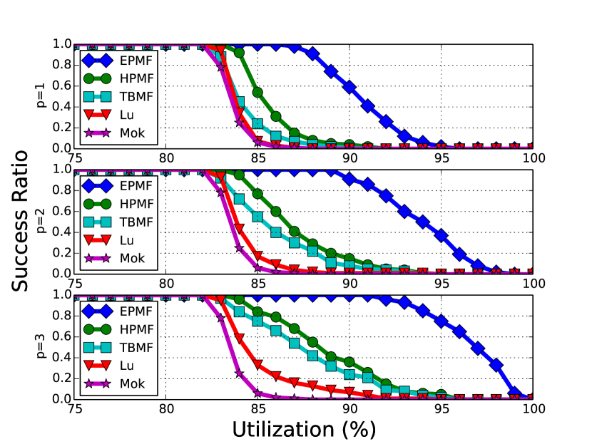
Figure 2: Success ratio comparison in multiframe systems

In this experiment, the proposed tests (the first three) and the existing tests are listed as follows:

• Extreme Points Multiframe test (EPMF): by using Lemma 4 in Theorem 7.

• Hyperbolic Bound MultiFrame (HPMF): Eq. (49).

• Total utilization Bound MultiFrame (TBMF): Eq. (50).

• Mok: Theorem 7 by Mok and Chen in [35].

• Lu: Theorem 3 by Lu et al. in [32].

Figure 2 presents the result for the performance in terms of the success ratio. For all tests, the success ratio are slightly better when the order of magnitude is greater. Our proposed tests are superior than the others for all different settings of $p$.

Note that the experiment conducted in [32] applies the technique of task merging proposed in [23] as a preprocess and then tests the utilization bound. Apparently, the former can be also used in our proposed tests. However, we do not adopt this prepocess in our evaluations but focus on the effectiveness of utilization bounds themselves instead. The conclusion remains the same after adopting the preprocess on both sides.

Evaluations for DAG Task Systems

Similarly, the DAG tasks were converted from the sporadic tasks as follows: The critical-path length $\Psi_{i}$ of task $\tau_{i}$ was set by multiplying its WCET by uniform random values in the range $[0.75,1]$. The following tests for global RM are evaluated:

• Extreme Points DAG test (EPDAG): by using the following testing $\frac{\Psi_{k}+\frac{C_{k}-\Psi_{k}}{M}}{T_{k}}\leq 1-\sum_{i=1}^{k-1}\frac{U_{i}(\alpha_{i}+\beta_{i})}{\prod_{j=i}^{k-1}(\beta_{j}U_{j}+1)}$ derived from Lemma 4, where $\alpha_{i}$ is defined as $\frac{2}{M}$ and $\beta_{i}$ as $\frac{1}{M}/\left\lfloor{\frac{T_{k}}{T_{i}}}\right\rfloor$.

• Hyperbolic Bound DAG (HPDAG): in Theorem 4.

• Chen and Agrawal Bound (CAB): in Corollary 4 in [13]. CAB has the best known capacity augmentation bound for DAG systems under global RM.

The cardinality of the task set was 50.

Figure 3 depicts results with different numbers of processors, i.e., $M=2,4,8$. For these algorithms, the success ratios are better when the number of processors is less. Apparently, our proposed tests are better than CAB, especially when the number of processors is large.

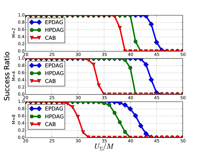
Figure 3: Success ratio comparison in DAG systems where $U_{\Sigma}$ is the total utilization of a DAG task set.

Evaluations for Implicit-Deadline Systems

These tests in this experiment are as follows:

• Extreme Points test (EP): We use Lemma 4 in the analysis in Sec. 5.1.

• Hyperbolic Bound (HP): in Corollary 1.

• Bini: in Corollary 2 in [8].

The cardinality of the task set was 10.

Figure 4 depicts the results for 3 different orders of magnitude, i.e., $p=1,2,3$. For there tests, the success ratio is better if the order of magnitude is greater. The EP dominates all the other tests for all different orders of magnitude. On the other hand, the results from Bini et al. in [8] and the proposed hyperbolic bound in Corollary 1 are comparable. The performance by the proposed hyperbolic bound is better than by Bini et al. in [8] for a smaller $p$ whereas Bini outperforms the proposed hyperbolic bound for a larger $p$.

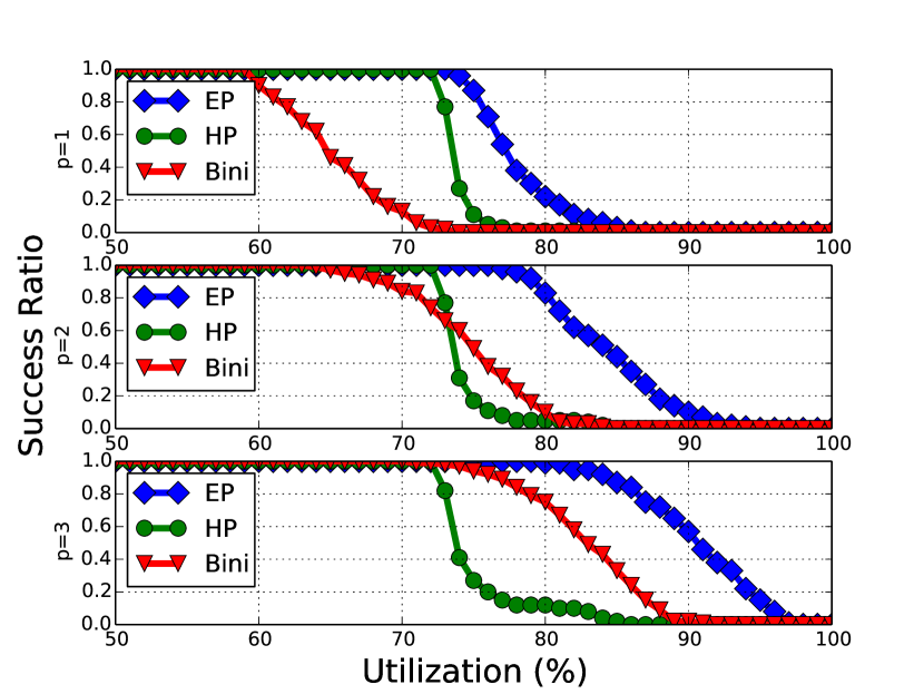
Figure 4: Success ratio comparison in implicit-deadline systems.

Appendix E: Additional Properties in $\mathbf{k^{2}U}$

We provide some additional properties that come directly from the $\mathbf{k^{2}U}$ framework. These properties were not directly used in any of the above demonstrated examples. The first lemma is useful when the index of the $k-1$ higher priority tasks is not provided and cannot be determined while applying the schedulability tests. The results in Section 4 highly rely on the given order of the $k-1$ tasks. Therefore, without the given ordering, to be safe, we have to test all the permutations of the ordering of the $k-1$ tasks. Fortunately, the following lemma, as an extension of Lemma 4, shows that testing only one particular ordering is enough to provide a safe schedulability test.

Lemma 10.

Suppose that the given $k$-point effective schedulability test, defined in Eq. (4), of a fixed-priority scheduling algorithm does not have a predefined order to index the $k-1$ higher-priority tasks. Task $\tau_{k}$ is schedulable by the scheduling algorithm if the following condition holds

$$0<\frac{C_{k}}{t_{k}}\leq 1-\sum_{i=1}^{k-1}\frac{U_{i}(\alpha_{i}+\beta_{i})}{\prod_{j=i}^{k-1}(\beta_{j}U_{j}+1)},$$ (53)

by indexing the $k-1$ higher-priority tasks in a non-decreasing order of $\frac{\alpha_{i}}{\beta_{i}}$, in which $0<t_{k}$ and $0<\alpha_{i}$ and $0<\beta_{i}$ for any $i=1,2,\ldots,k-1$.

Proof. This lemma is proved by showing that the schedulability condition in Lemma 4, i.e., $1-\sum_{i=1}^{k-1}\frac{U_{i}(\alpha_{i}+\beta_{i})}{\prod_{j=i}^{k-1}(\beta_{j}U_{j}+1)}$, is minimized, when the $k-1$ higher-priority tasks are indexed in a non-decreasing order of $\frac{\alpha_{i}}{\beta_{i}}$. Suppose that there are two adjacent tasks $\tau_{\ell}$ and $\tau_{\ell+1}$ with $\frac{\alpha_{\ell}}{\beta_{\ell}}>\frac{\alpha_{\ell+1}}{\beta_{\ell+1}}$. Let’s now examine the difference of $\sum_{i=1}^{k-1}\frac{U_{i}(\alpha_{i}+\beta_{i})}{\prod_{j=i}^{k-1}(\beta_{j}U_{j}+1)}$ by swapping the index of task $\tau_{\ell}$ and task $\tau_{\ell+1}$. It can be easily observed that the other tasks $\tau_{i}$ with $i\neq\ell$ and $i\neq\ell+1$ do not change their corresponding values $\frac{U_{i}(\alpha_{i}+\beta_{i})}{\prod_{j=i}^{k-1}(\beta_{j}U_{j}+1)}$ in both orderings (before and after swapping $\tau_{\ell}$ and $\tau_{\ell+1}$). Suppose that $\frac{1}{\prod_{j=\ell}^{k-1}(\beta_{j}U_{j}+1)}$ is $Q$, in which $Q>0$. The difference in the term $\sum_{i=1}^{k-1}\frac{U_{i}(\alpha_{i}+\beta_{i})}{\prod_{j=i}^{k-1}(\beta_{j}U_{j}+1)}$ before and after swapping tasks $\tau_{\ell}$ and $\tau_{\ell+1}$ is

$$\left((\alpha_{\ell}+\beta_{\ell})U_{\ell}Q+(\alpha_{\ell+1}+\beta_{\ell+1})U_{\ell+1}Q(1+\beta_{\ell}U_{\ell})\right)$$

$$-\left((\alpha_{\ell+1}+\beta_{\ell+1})U_{\ell+1}Q+(\alpha_{\ell}+\beta_{\ell})U_{\ell}Q(1+\beta_{\ell+1}U_{\ell+1})\right)$$

$$= U_{\ell}U_{\ell+1}Q(\beta_{\ell}\alpha_{\ell+1}-\beta_{\ell+1}\alpha_{\ell})$$

$$= \beta_{\ell}\beta_{\ell+1}U_{\ell}U_{\ell+1}Q\left(\frac{\alpha_{\ell+1}}{\beta_{\ell+1}}-\frac{\alpha_{\ell}}{\beta_{\ell}}\right)<0.$$

Therefore, we reach the conclusion by repetitively swapping the tasks to achieve a non-decreasing order of $\frac{\alpha_{i}}{\beta_{i}}$ for maximizing $\sum_{i=1}^{k-1}\frac{U_{i}(\alpha_{i}+\beta_{i})}{\prod_{j=i}^{k-1}(\beta_{j}U_{j}+1)}$.        

Based on Lemma 10, if all the $k-1$ higher-priority tasks have a constant $\beta_{i}=\beta>0$, we know that they should be indexed in a non-decreasing order of $\alpha_{i}$. There are also cases, in which we only know that the $k-1$ higher-priority tasks can be classified such that $h$ of them are associated with $\alpha_{i}=\alpha^{\sharp}$ and the other $k-1-h$ tasks are associated with $\alpha_{i}=\alpha^{\flat}$. This means that we are not sure whether task $\tau_{i}$ should be associated with $\alpha^{\sharp}$ or $\alpha^{\flat}$. Instead of testing all possible combinations, the following lemma shows that we only have to index the $k-1$ higher-priority tasks by their utilization non-decreasingly.

Lemma 11.

Suppose that the $k$-point effective schedulability test, defined in Eq. (4), of a fixed-priority scheduling algorithm is defined with (1) a constant $\beta_{i}=\beta>0$ for all the $k-1$ higher priority tasks and (2) uncertain $h$ higher-priority tasks ($h<k-1$) associated with $\alpha^{\sharp}$ and the remaining $k-1-h$ tasks with $\alpha^{\flat}$, where $\alpha^{\sharp}>\alpha^{\flat}>0$. Task $\tau_{k}$ is schedulable by the scheduling algorithm if the following condition holds

$$0<\frac{C_{k}}{t_{k}}\leq 1-\sum_{i=1}^{k-1}\frac{U_{i}(\alpha_{i}+\beta)}{\prod_{j=i}^{k-1}(\beta U_{j}+1)},$$ (54)

by indexing the $k-1$ higher-priority tasks in a non-decreasing order of $U_{i}$ and assigning $\alpha_{1},\alpha_{2},\ldots,\alpha_{k-1-h}$ to $\alpha^{\flat}$ and $\alpha_{k-h},\alpha_{k-h+1},\ldots,\alpha_{k-1}$ to $\alpha^{\sharp}$.

Proof. The assignment of the $\alpha_{i}$ values is due to Lemma 10. Suppose $U_{\ell}>U_{\ell+1}$ for a certain $\ell$. There are three cases: (1) $\ell<k-1-h$, (2) $\ell=k-1-h$, and (3) $\ell>k-1-h$. For the first and the third cases, swapping the assignment of the utilization does not change the right-hand side of Eq. (54). Only the second case matters. When $\ell=k-1-h$, it can be easily observed that due to the assumption $U_{\ell}>U_{\ell+1}$ and $\alpha_{\ell}<\alpha_{\ell+1}$, the right-hand side of Eq. (54) after swapping the assignment of the utilization (without swapping $\alpha_{\ell}$ and $\alpha_{\ell+1}$) is reduced. Therefore, the swapping makes the test harder. As a result, by repeating the above procedure, we reach the conclusion.        

We will demonstrate how to use Lemma 11 in Appendix F for deriving a more precise hyperbolic bound with respect to global RM scheduling. The above lemma can be further generalized by allowing more levels of $\alpha_{i}$ values with a minor extension. However, there is no concrete clue whether such an extension may be useful. The following lemmas provide the utilization bound of Lemma 2 for the case $\alpha+\beta>1$.

Lemma 12.

Suppose that $\alpha+\beta>1$. For a given $k$-point effective schedulability test of a scheduling algorithm, defined in Definition 1, in which $0<t_{k}$ and $0<\alpha_{i}\leq\alpha$ and $0<\beta_{i}\leq\beta$ for any $i=1,2,\ldots,k-1$, task $\tau_{k}$ is schedulable by the scheduling algorithm if

$$\small\frac{C_{k}}{t_{k}}+\sum_{i=1}^{k-1}U_{i}\leq\begin{cases}\frac{\ln(1+\frac{\beta}{\alpha})}{\beta},&(\alpha+\beta)^{\frac{1}{k}}<\alpha\\ \frac{\ln(\alpha+\beta)-\alpha+1}{\beta},&\mbox{otherwise.}\\ \end{cases}$$ (55)

Proof. With the assumption $\alpha+\beta>1$, we only have to consider the last two cases in Eq. (16). In both cases, the minimum bound happens when $k$ goes to $\infty$. For the case with $\frac{(k-1)((1+\frac{\beta}{\alpha})^{\frac{1}{k-1}}-1)}{\beta}$, this is lower bounded by $\frac{\ln(1+\frac{\beta}{\alpha})}{\beta}$ when $k\rightarrow\infty$. For the other case, we have $\frac{(k-1)((\alpha+\beta)^{\frac{1}{k}}-1)+((\alpha+\beta)^{\frac{1}{k}}-\alpha)}{\beta}=\frac{k((\alpha+\beta)^{\frac{1}{k}}-1)+1-\alpha}{\beta}$.        

Lemma 13.

Suppose that $\alpha+\beta>1$. For a given $k$-point effective schedulability test of a scheduling algorithm, defined in Definition 1, in which $0<t_{k}$ and $0<\alpha_{i}\leq\alpha$ and $0<\beta_{i}\leq\beta$ for any $i=1,2,\ldots,k-1$, task $\tau_{k}$ is schedulable by the scheduling algorithm if

$$\small\frac{1}{\alpha}\frac{C_{k}}{t_{k}}+\sum_{i=1}^{k-1}U_{i}\leq\frac{k((1+\frac{\beta}{\alpha})^{\frac{1}{k}}-1)}{\beta},$$ (56)

in which the right-hand side of Eq. (56) is lower bounded by $\frac{\ln(1+\frac{\beta}{\alpha})}{\beta}$ when $k\rightarrow\infty$.

Proof. This comes directly from Eq. (5) in Lemma 1 with a simpler Lagrange Multiplier procedure. That is, the infimum $\frac{1}{\alpha}\frac{C_{k}}{t_{k}}+\sum_{i=1}^{k-1}U_{i}$ with $(\frac{C_{k}}{t_{k}}+\frac{\alpha}{\beta})(\beta U_{1}+1)^{k-1}>\frac{\alpha}{\beta}+1$ happens when $\frac{\beta}{\alpha}\frac{C_{k}}{t_{k}}=\beta U_{1}=\beta U_{2}=\cdots=\beta U_{k-1}=((1+\frac{\beta}{\alpha})^{\frac{1}{k}}-1)$.        

With Lemma 13, the first case in Eq. (55) already pessimistically holds when $\alpha\geq 1$. The above two lemmas generalize the results in [30] for the case $1\leq\alpha\leq 2$ and $\beta=1$.

Appendix F: Improved Global RM Test

The test in Section 6 of global RM scheduling for sporadic tasks can be improved by using a tighter schedulability test from Guan et al. [21]. It has been concluded by Guan et al. [21] that we only have to consider $M-1$ tasks with carry-in jobs, for constrained-deadline task sets, when considering task $\tau_{k}$ with $k>M$. For implicit-deadline task sets, this means that we only need to set $\alpha_{i}$ of some tasks to $\frac{2}{M}$, rather than all the $k-1$ tasks in Eq. (29). More precisely, we can define two different time-demand functions, depending on whether task $\tau_{i}$ is with a carry-in job or not:

$$W_{i}^{carry}(t)=\begin{cases}C_{i}&0<t<C_{i}\\ C_{i}+\left\lceil{\frac{t-C_{i}}{T_{i}}}\right\rceil C_{i}&otherwise,\end{cases}$$ (57)

and

$$W_{i}^{normal}(t)=\left\lceil{\frac{t}{T_{i}}}\right\rceil C_{i}.$$ (58)

Moreover, we can further over-approximate $W_{i}^{carry}(t)$, since $W_{i}^{carry}(t)\leq W_{i}^{normal}(t)+C_{i}$. Therefore, a sufficient schedulability test for testing task $\tau_{k}$ with $k>M$ for global RM is to verify whether

$$\exists 0<t\leq T_{k},C_{k}+\frac{(\sum_{\tau_{i}\in{\bf T}^{\prime}}C_{i})+(\sum_{i=1}^{k-1}W_{i}^{normal}(t))}{M}\leq t.$$ (59)

for all ${\bf T}^{\prime}\subseteq hp(\tau_{k})$ with $|{\bf T}^{\prime}|=M-1$. That is, if the above test in Eq. (59) passes for any selection of $M-1$ higher-priority tasks to have carry-in jobs, then task $\tau_{k}$ is schedulable by global RM. For a given carry-in task set ${\bf T}^{\prime}$ with $|{\bf T}^{\prime}|=M-1$, the translation to the $\mathbf{k^{2}U}$ framework is as follows: (1) the parameters are $0<\alpha_{i}\leq\frac{2}{M}$ and $0<\beta_{i}\leq\frac{1}{M}$ by using Eq. (59) if $\tau_{i}$ is in ${\bf T}^{\prime}$, and (2) the parameters are $\alpha_{i}=\frac{1}{M}$ and $0<\beta_{i}\leq\frac{1}{M}$ by using Eq. (59) if $\tau_{i}$ is not in ${\bf T}^{\prime}$. Therefore, this is exactly the case when Lemma 11 can be adopted by selecting $M-1$ higher-priority tasks with $\alpha_{i}=\frac{2}{M}$ and the remaining $k-M$ higher-priority tasks with $\alpha_{i}=\frac{1}{M}$, where $\beta_{i}$ is set safely to $\frac{1}{M}$. Therefore, we reach the conclusion with the following theorem by the above analysis and Lemma 11.

Theorem 9.

Task $\tau_{k}$ with $k>M$ in a sporadic implicit-deadline task system is schedulable by global RM on $M$ processors if

$$0<U_{k}\leq 1-\sum_{i=1}^{k-1}\frac{U_{i}(\alpha_{i}+\frac{1}{M})}{\prod_{j=i}^{k-1}(\frac{1}{M}U_{j}+1)},$$ (60)

by indexing the $k-1$ higher-priority tasks in a non-decreasing order of $U_{i}$ and assigning $\alpha_{1},\alpha_{2},\ldots,\alpha_{k-M}$ to $\frac{1}{M}$ and $\alpha_{k-M+1},\alpha_{k-M+2},\ldots,\alpha_{k-1}$ to $\frac{2}{M}$.

References

• [1] B.Β Andersson, S.Β K. Baruah, and J.Β Jonsson. Static-priority scheduling on multiprocessors. In Real-Time Systems Symposium (RTSS), pages 193–202, 2001.
• [2] T.Β P. Baker. Multiprocessor EDF and deadline monotonic schedulability analysis. In IEEE Real-Time Systems Symposium, pages 120–129, 2003.
• [3] S.Β Baruah, V.Β Bonifaci, and A.Β Marchetti-Spaccamela. The global EDF scheduling of systems of conditional sporadic DAG tasks. In ECRTS, pages 222–231, 2015.
• [4] S.Β K. Baruah, A.Β K. Mok, and L.Β E. Rosier. Preemptively scheduling hard-real-time sporadic tasks on one processor. In IEEE Real-Time Systems Symposium, pages 182–190, 1990.
• [5] M.Β Bertogna, M.Β Cirinei, and G.Β Lipari. New schedulability tests for real-time task sets scheduled by deadline monotonic on multiprocessors. In Principles of Distributed Systems, 9th International Conference, OPODIS, pages 306–321, 2005.
• [6] E.Β Bini and G.Β C. Buttazzo. Measuring the performance of schedulability tests. Real-Time Systems, 30(1-2):129–154, 2005.
• [7] E.Β Bini, G.Β C. Buttazzo, and G.Β M. Buttazzo. Rate monotonic analysis: the hyperbolic bound. Computers, IEEE Transactions on, 52(7):933–942, 2003.
• [8] E.Β Bini, T.Β H.Β C. Nguyen, P.Β Richard, and S.Β K. Baruah. A response-time bound in fixed-priority scheduling with arbitrary deadlines. IEEE Transactions on Computers, 58(2):279, 2009.
• [9] V.Β Bonifaci, A.Β Marchetti-Spaccamela, S.Β Stiller, and A.Β Wiese. Feasibility analysis in the sporadic dag task model. In ECRTS, pages 225–233, 2013.
• [10] A.Β Burchard, J.Β Liebeherr, Y.Β Oh, and S.Β H. Son. New strategies for assigning real-time tasks to multiprocessor systems. pages 1429–1442, 1995.
• [11] S.Β Chakraborty, S.Β KΓΌnzli, and L.Β Thiele. Approximate schedulability analysis. In IEEE Real-Time Systems Symposium, pages 159–168, 2002.
• [12] J.-J. Chen. Partitioned multiprocessor fixed-priority scheduling of sporadic real-time tasks. Computing Research Repository (CoRR), abs/1505.04693, 2015.
• [13] J.-J. Chen and K.Β Agrawal. Capacity augmentation bounds for parallel dag tasks under G-EDF and G-RM. Technical Report 845, Faculty for Informatik at TU Dortmund, 2014.
• [14] J.-J. Chen, W.-H. Huang, and C.Β Liu. Evaluate and compare two utilization-based schedulability-test frameworks for real-time systems. Computing Research Repository (CoRR), abs/1505.02155, 2015.
• [15] J.-J. Chen, W.-H. Huang, and C.Β Liu. $k^{2}Q$: A quadratic-form response time and schedulability analysis framework for utilization-based analysis. Computing Research Repository (CoRR), abs/1505.03883, 2015.
• [16] R.Β Davis and A.Β Burns. A survey of hard real-time scheduling for multiprocessor systems. Journal of ACM Computing Surveys, 43(4)(35), 2011.
• [17] R.Β Davis, T.Β Rothvoß, S.Β Baruah, and A.Β Burns. Quantifying the sub-optimality of uniprocessor fixed priority pre-emptive scheduling for sporadic tasksets with arbitrary deadlines. In Real-Time and Network Systems (RTNS), pages 23–31, 2009.
• [18] R.Β I. Davis, T.Β Rothvoß, S.Β K. Baruah, and A.Β Burns. Exact quantification of the sub-optimality of uniprocessor fixed priority pre-emptive scheduling. Real-Time Systems, 43(3):211–258, 2009.
• [19] R.Β I. Davis, A.Β Zabos, and A.Β Burns. Efficient exact schedulability tests for fixed priority real-time systems. Computers, IEEE Transactions on, 57(9):1261–1276, 2008.
• [20] N.Β Fisher and S.Β K. Baruah. A fully polynomial-time approximation scheme for feasibility analysis in static-priority systems with arbitrary relative deadlines. In ECRTS, pages 117–126, 2005.
• [21] N.Β Guan, M.Β Stigge, W.Β Yi, and G.Β Yu. New response time bounds for fixed priority multiprocessor scheduling. In IEEE Real-Time Systems Symposium, pages 387–397, 2009.
• [22] C.-C. Han and H.-Y. Tyan. A better polynomial-time schedulability test for real-time fixed-priority scheduling algorithms. In Real-Time Systems Symposium (RTSS), pages 36–45, 1997.
• [23] T.-W. Kuo, L.-P. Chang, Y.-H. Liu, and K.-J. Lin. Efficient online schedulability tests for real-time systems. Software Engineering, IEEE Transactions on, 29(8):734–751, 2003.
• [24] C.-G. Lee, L.Β Sha, and A.Β Peddi. Enhanced utilization bounds for QoS management. IEEE Trans. Computers, 53(2):187–200, 2004.
• [25] J.Β P. Lehoczky. Fixed priority scheduling of periodic task sets with arbitrary deadlines. In RTSS, pages 201–209, 1990.
• [26] J.Β P. Lehoczky, L.Β Sha, and Y.Β Ding. The rate monotonic scheduling algorithm: Exact characterization and average case behavior. In IEEE Real-Time Systems Symposium, pages 166–171, 1989.
• [27] J.Β Y.-T. Leung and J.Β Whitehead. On the complexity of fixed-priority scheduling of periodic, real-time tasks. Perform. Eval., 2(4):237–250, 1982.
• [28] J.Β Li, J.Β Chen, K.Β Agrawal, C.Β Lu, C.Β Gill, and A.Β Saifullah. Analysis of federated and global scheduling for parallel real-time tasks. In Euromicro Conference on Real-Time Systems, 2014.
• [29] C.Β Liu and J.Β Anderson. Task scheduling with self-suspensions in soft real-time multiprocessor systems. In Proceedings of the 30th Real-Time Systems Symposium, pages 425–436, 2009.
• [30] C.Β Liu and J.-J. Chen. Bursty-interference analysis techniques for analyzing complex real-time task models. In IEEE Real-Time Systems Symposium, 2014.
• [31] C.Β L. Liu and J.Β W. Layland. Scheduling algorithms for multiprogramming in a hard-real-time environment. Journal of the ACM (JACM), 20(1):46–61, 1973.
• [32] W.-C. Lu, K.-J. Lin, H.-W. Wei, and W.-K. Shih. New schedulability conditions for real-time multiframe tasks. In ECRTS, pages 39–50. IEEE, 2007.
• [33] D.Β G. Luenberger and Y.Β Ye. Linear and nonlinear programming, volume 116. Springer, 2008.
• [34] A.Β K. Mok. Fundamental design problems of distributed systems for the hard-real-time environment. 1983.
• [35] A.Β K. Mok and D.Β Chen. A multiframe model for real-time tasks. IEEE Trans. Software Eng., pages 635–645, 1997.
• [36] G.Β vonΒ der Bruggen, J.-J. Chen, and W.Β Huang. Schedulability and optimization analysis for non-preemptive static priority scheduling based on task utilization and blocking factors. In ECRTS, pages 90–101, 2015.
• [37] J.Β Wu, J.Β Liu, and W.Β Zhao. On schedulability bounds of static priority schedulers. In Real-Time and Embedded Technology and Applications Symposium (RTAS), pages 529–540, 2005.