Dynamical many-body phases of the parametrically driven, dissipative Dicke model

Abstract

The dissipative Dicke model exhibits a fascinating out-of-equilibrium many-body phase transition as a function of a coupling between a driven photonic cavity and numerous two-level atoms. We study the effect of a time-dependent parametric modulation of this coupling, and discover a rich phase diagram as a function of the modulation strength. We find that in addition to the established normal and super-radiant phases, a new phase with pulsed superradiance which we term dynamical normal phase appears when the system is parametrically driven. Employing different methods, we characterize the different phases and the transitions between them. Specific heed is paid to the role of dissipation in determining the phase boundaries. Our analysis paves the road for the experimental study of dynamically stabilized phases of interacting light and matter.

Experimental progress in control and manipulation of light-matter quantum systems has generated a growing interest in many-body phenomena out of equilibrium Carusotto and Ciuti (2013). Well established examples of such systems include ultracold atomic or ionic quantum gases in high finesse optical cavities Bloch et al. (2008), semiconductor microcavities in the strong coupling regime Kavokin et al. (2007); Carusotto and Ciuti (2013), and superconducting qubits in microwave resonators Wallraff et al. (2004); Majer et al. (2007). The engineered interplay between light and matter in these systems has led to the observation of a host of fascinating collective phases and quantum phase transitions including superfluidity in polaritons Amo et al. (2009) and the super-radiant Dicke phase transition in a Bose-Einstein condensate (BEC) coupled to an optical cavity Brennecke et al. (2013).

A defining feature of many of these systems is that they are inherently driven and subject to dissipation. Driven dissipative systems are usually treated within a rotating frame formalism. This effectively renders the problem time-independent with the important feature that the asymptotic steady states are necessarily out of equilibrium. However, parametric driving of the system often does not allow the usual rotating frame simplifications. Consequently, the resulting interplay between interactions, dissipation, and parametric driving, could lead to novel and exotic steady-state physics that has no counterpart in the undriven case. Parametric driving is increasingly used as an experimental tool in diverse contexts, e.g. , in the generation of Floquet topological insulators Rechtsman et al. (2013), improved measurement fidelity with squeezed quantum states Orzel et al. (2001); Rugar et al. (2004) and unconventional phenomena in cavity QED Günter et al. (2009).

A prime example of a system exhibiting light-matter collective phenomenon is the Dicke model Dimer et al. (2007). Here, a bosonic/cavity mode is coupled to a large number of two-level atoms. It exhibits a $Z_{2}$ symmetry breaking quantum phase transition from a normal phase (NP), where all the atoms are in their ground state and the cavity is empty, to a super-radiant phase (SP), where the atoms are excited and the cavity is in a coherent state. This model has recently been realized by coupling the external degree of freedom of a BEC to a quantized mode of a laser-driven optical cavity, and the theoretically predicted non-equilibrium phase transition has been observed Brennecke et al. (2013); Klinder et al. (2014). Moreover, the inevitable photon leakage out of the cavity as well as dissipation of the BEC has been shown to lead to a considerable modification of the critical exponents of the transition Nagy et al. (2011).

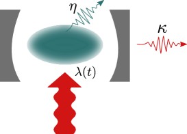
Figure 1: A sketch of a parametrically driven Dicke model. A single-mode cavity is driven by a laser beam with an oscillating laser-field power $P(t)$. The cavity is naturally leaky with a dissipation rate $\kappa$. Inside the cavity, an atomic cloud is cooled and forms a Bose-Einstein condensate that is coupled to the driving laser with coupling $\lambda(t)\propto\sqrt{P(t)}$ [cf. Eq. (1)]. The atoms are also coupled to an environment with a dissipation rate $\eta$. The system is best described by Liouvillian dynamics [cf. Eq. (2)].

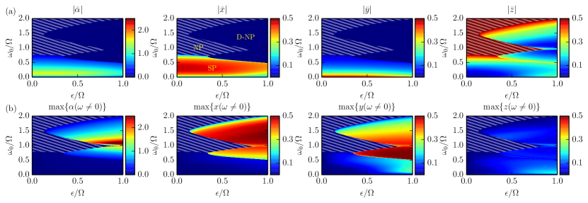
Figure 2: Characteristics of the dynamical phase diagram of the parametrically driven Dicke model as a function of cavity/atoms frequency $\omega_{0}=\omega_{c}=\omega_{a}$ and parametric modulation strength $\epsilon$ for bare coupling $\lambda_{0}=0.4\Omega$ and dissipation rates $\kappa=\eta=0.1\Omega$. We obtain these characteristics from the numerical steady-state solutions of the mean field equations [cf. Eqs. (6)-(8)]. Each point, with a $10^{-3}$ resolution, is a result of a different numerical integration. Superimposed (striped overlay) is the normal mode stability zone [cf. Eq. (5)]. (a) Density plots of the absolute value of the steady-state time-averaged order parameters. (b) In steady-state the order parameters are oscillating with a complex beat structure sup . The density plots are of the amplitude of the maximal frequency $\omega$ contributing to this oscillation. We see three distinct phases appearing as a function of $\epsilon$, i.e. , extensions of the normal and super-radiant phases (NP and SP), as well as a novel dynamical phase (D-NP). These three phases meet at a shared multicritical point. The properties of each phase are summarized in Table 1.

In this work, we analyze the impact of parametric driving on the phase diagram of the dissipative Dicke model. Specifically, we consider a modulation of the atom-cavity coupling, which is easily realizable in current experimental setups, see Fig. 1. Using a combination of mean field theory and effective Hamiltonians, we obtain a rich phase diagram comprising: (i) the NP with parametric amplification, (ii) the SP phase, and (iii) a novel dynamical normal phase (D-NP), which appears to be a dynamically rotating NP with pulsed super-radiance. We elucidate the vital role that dissipation plays in modifying the complex phase topography of this nonequilibrium system. Our analysis presents parametric driving as a promising frontier in the search for exotic collective phases in light-matter systems.

The single mode parametrically driven Dicke model is described by the Hamiltonian

$$H(t)=\hbar\omega_{c}a^{\dagger}a+\hbar\omega_{a}\sum_{i=1}^{N}s_{z}^{i}+{\frac{2\hbar\lambda(t)}{\sqrt{N}}}\sum_{i=1}^{N}s_{x}^{i}(a+a^{\dagger})\,,$$ (1)

where $s^{i}_{\alpha}$ with $\alpha=x,y,z$ are the spin operators describing the $i^{\rm th}$ two level atom, and $a,a^{\dagger}$ represent the cavity creation and annihilation operators. The cavity’s resonance frequency is $\omega_{c}$, whereas the atoms are considered to be identical with level spacing $\hbar\omega_{a}$. We consider a time-dependent coupling between the atoms and the cavity of the form $\lambda(t)=\lambda_{0}+\epsilon\cos(2\Omega t)$. Such a coupling is easily generated by a modulation of the laser power that drives the cavity eps . For $\epsilon=0$, the system exhibits the well known continuous phase transition from a NP to a SP when the coupling $\lambda_{0}\geq\sqrt{\omega_{c}\omega_{a}}/2$ Dimer et al. (2007). For $\epsilon\neq 0$, we reiterate that the parametric driving described here cannot be rotated away by a suitable choice of frame. Indeed, recent treatments of similar modulations of the Dicke model were addressed using a mapping to parametric oscillators, and a partial phase diagram for the NP was obtained Bastidas et al. (2012); Vacanti et al. (2012). Here, we explicitly include dissipation for both the cavity and the atoms (see Fig. 1) and analyze the impact of parametric driving on the full phase diagram of the dissipative Dicke model, see Fig. 2.

The driven and dissipative nature of the system is described by a Liouvillian equation for the density matrix $\rho_{\rm sys}$ of the system

$$\frac{d\rho_{\rm sys}}{dt} = -\frac{i}{\hbar}[H(t),\rho_{\rm sys}]+\kappa[2a\rho_{\rm sys}a^{\dagger}-\{a^{\dagger}a,\rho_{\rm sys}\}]$$ (2)

$$+\frac{\eta}{N}\sum_{i,j=1}^{N}[2s^{i}_{-}\rho_{\rm sys}s_{+}^{j}-\{s^{i}_{+}s^{j}_{-},\rho_{\rm sys}\}]\,,$$

where $s_{\pm}^{j}=s_{x}^{j}+is_{y}^{j}$ are ladder operators. The first term on the r.h.s. describes the standard Hamiltonian evolution and the last two terms represent the Markovian dissipation for both cavity and a global dissipation for the atoms in Lindblad form with rates $\kappa$ and $\eta$, respectively Shirai et al. (2014). Note that this approach is valid in the Born-Markov limit of weak dissipation.

	Stability $A_{1}$	Stability $A_{2}$	$\left|\bar{\alpha}\right|$	$\left|\bar{x}\right|$	$\left|\bar{y}\right|$	$\left|\bar{z}\right|$
NP	yes	yes	0	0	0	1/2
SP	no	yes	$\neq 0$	$\neq 0$	$\neq 0$	$\neq 0$
D-NP	no ($\star$)	no ($\star$)	$0$	$0$	$0$	$<1/2$

Table 1: Summary of normal mode [cf. Eq. (5)] and mean field [cf. Eqs. (6)-(8)] analyses. In Fig. 2(a), we observe three main regions, dubbed normal phase (NP), super-radiant phase (SP), and dynamical normal phase (D-NP). Each region manifests a different behavior summarized here, i.e. , which normal mode is stable in each region sup , and what are the values of the different order parameters. In the D-NP region, we denote by “no ($\star$)” that at least one normal mode is unstable.

In the absence of paramteric driving, $\epsilon=0$, the NP is well described by considering the collection of two-level atoms as constituting a giant spin ${\bf S}=\sum_{i}{\bf s}^{i}$ aligned along the $z$ axis Emary and Brandes (2003). The deviations of this giant spin away from this quantization axis can be characterized by the standard Holstein Primakoff representation for the spin operators, $S_{z}=b^{\dagger}b-{\frac{N}{2}},S_{-}=\sqrt{N-b^{\dagger}b}b$, and $S_{+}=b^{\dagger}\sqrt{N-b^{\dagger}b}$, where $b,b^{\dagger}$ are standard bosonic operators Emary and Brandes (2003). This approach can be extended to address the stability of the NP in the presence of parametric driving, $\epsilon\neq 0$. Since deviations of $\mathbf{S}$ from the $z$ axis are expected to be small, as $N\to\infty$ we can map the Dicke Hamiltonian [cf. Eq. (1)] onto the problem of two harmonic oscillators whose coupling is parametrically driven,

$$H_{\rm NP}(t)=\hbar\omega_{c}a^{\dagger}a+\hbar\omega_{a}b^{\dagger}b+\hbar\lambda(t)(b+b^{\dagger})(a+a^{\dagger})\,.$$ (3)

Focusing on the case $\omega_{0}\equiv\omega_{a}=\omega_{c}$, Eq. (3) can be diagonalized in terms of normal modes,

$$H_{\rm NP}(t)=\hbar\Omega_{1}(t)A_{1}^{\dagger}A_{1}+\hbar\Omega_{2}(t)A_{2}^{\dagger}A_{2}\,,$$ (4)

where for $m=1,2$, $\Omega_{m}^{2}(t)=\omega_{0}^{2}-(-1)^{m}2\lambda(t)\omega_{0}$ are time-dependent normal mode frequencies, and $A_{m}=\frac{1}{2\sqrt{2}}[\mathcal{S}^{+}_{m}(a-(-1)^{m}b)+\mathcal{S}^{-}_{m}(a^{\dagger}-(-1)^{m}b^{\dagger})]$ are the corresponding normal mode operators with coefficients $\mathcal{S}_{m}^{\pm}=\frac{\Omega_{m}\pm\omega_{0}}{2\sqrt{\omega_{0}\Omega_{m}}}$. For computational simplicity, we also assume $\kappa=\eta\equiv\gamma$Galve et al. (2010).

Each normal mode is a quantum Mathieu parametric oscillator, i.e. , its fundamental harmonic frequency varies sinusoidally in time McLachlan (1964); Nayfeh and Mook (1979). The stability of each quantum parametric oscillator can be deduced from its displacement ${\rm Tr}\left\{\rho(t)(A_{m}+A_{m}^{\dagger})\right\}$. It results in a complex stability diagram comprising “Arnold tongues” which delineate regions where the displacement, though parametrically amplified, remains bounded (stable), and those where the displacement grows exponentially with time (unstable) Zerbe et al. (1994); Zerbe and Hänggi (1995); sup . Incidentally, the resulting stability diagram for the quantum oscillator is the same as that of the classical damped Mathieu oscillator obeying the classical equations of motion for the displacementZerbe et al. (1994); Zerbe and Hänggi (1995); sup ,

$${\ddot{x}}_{m}+\gamma\dot{x}_{m}+\Omega_{m}^{2}(t)x_{m} = 0\,,$$ (5)

The combination of the stability diagrams of the two normal modes yields the stability of the NP, i.e. , the NP is stable only if both dissipative normal modes are stable, see shaded area in Fig. 2. In the absence of dissipation, $\kappa=\eta=\gamma=0$, each normal mode $A_{m}$ is unstable in the limit of infinitesimal parametric driving $\epsilon\rightarrow 0$ at resonant frequencies $f_{m,n}=\sqrt{(\lambda_{0})^{2}+n^{2}\Omega^{2}}+(-1)^{m}(\lambda_{0})$ where $n=1,2,3...$ McLachlan (1964); Nayfeh and Mook (1979). We find that the lower boundary of the NP is dictated by the lowest Arnold tongue of $A_{2}$, i.e. , where the time-independent part of $\Omega_{2}(t)$ becomes negative. The remaining stability boundaries of NP are determined by frequencies where either $A_{m}$ becomes unstable. The impact of disspation on the stability of NP can be understood from the physics of Mathieu oscillators where dissipation results in a modification of the stability criterion for the parametric oscillator. In particular, weak Markovian dissipation leads to a pronounced stabilization of the NP in the vicinity of these resonant frequencies for small driving $\epsilon\ll\lambda_{0}$, and barely affects the stability at higher drive amplitudes Zerbe et al. (1994); Zerbe and Hänggi (1995). Indeed in Fig. 2, we see substantial stabilization of NP at the resonant frequency $f_{2,1}$. Such stabilization of the NP in the many-body context of the Dicke model is a manifestation of the explicitly dissipation dependent non-equilibrium asymptotic state.

From Fig. 2, we see that the NP occupies only a small part of the phase diagram when the system is parametrically driven. However, what lies beyond these stable NP regions cannot be accessed by the current approach and requires another method, such as mean field theory, which is well justified for the Dicke model in the limit of $N\gg 1$. This method was successfully used for studying the SP which has broken $Z_{2}$ symmetry, for the non-driven case $\epsilon=0$ Hepp and Lieb (1973); Emary and Brandes (2003); Dimer et al. (2007). The mean field ansatz that we use states that the total density matrix in the steady state is a product state of the individual density matrices, $\rho_{\rm sys}=\rho_{c}\otimes\prod_{i=1}^{N}\otimes\rho_{i}$, where $\rho_{c}$ and $\rho_{i}$ are density matrices of the cavity and the $i^{\rm th}$ atom, respectively Shirai et al. (2014). Furthermore, since all atoms are identical, we assume all $\rho_{i}$ to be equivalent. Substituting this ansatz into Eq. (2), we obtain a set of coupled non-linear equations for the mean-field order parameters of the parametrically driven and dissipative Dicke model

$$\dot{\alpha}= -i\omega_{c}\alpha-2i\lambda(t)x-\kappa\alpha\,,$$ (6)

$${\dot{x}}= -\omega_{a}y-\eta x\,,$$ (7)

$${\dot{y}}= \omega_{a}x-2\lambda(t)[\alpha+\alpha^{*}]z-\eta y\,,$$ (8)

where we have defined the order parameters $\alpha=\langle a\rangle/\sqrt{N}$, $x=\langle\sum_{i}s^{x}_{i}\rangle/N$, $y=\langle\sum_{i}s^{y}_{i}\rangle/N$, $z=\langle\sum_{i}s^{z}_{i}\rangle/N$, and have assumed $z=\sqrt{(1/2)^{2}-|x|^{2}-|y|^{2}}$ since the mean field equations satisfy the constraint $x^{2}+y^{2}+z^{2}=1/4$.

Equations (6)-(8) form a set of coupled non-autonomous differential equations. Using numerical stiff ordinary differential equations solvers, we integrate this set of equations to a long time limit, where we obtain a convergent behavior. We find that, generically, the steady-state mean-field solutions show oscillatory behavior around a zero or non-zero mean value sup . In Figs. 2(a), we plot the absolute time-averaged order parameters, $|\bar{\alpha}|,|\bar{x}|,|\bar{y}|$ and $|\bar{z}|$, averaged over a sufficiently long time window in the steady-statesup . Note, that the absolute value is taken for presentation reasons only, we always have $\bar{\alpha},\bar{y},\bar{z}>0$ and $\bar{x}<0$. Based on these mean values, we find that the SP, characterized by $\bar{\alpha}\neq 0$, extends from its zero drive region of $\omega_{0}\leq 2\lambda_{0}$ onto a large regime spanning both small and large drive amplitudes. At the critical frequency $\omega_{\rm crit}(\omega_{0},\epsilon)$, we observe a transition to a region with $\bar{\alpha}=\bar{x}=\bar{y}=0$. Contrasting these results with those obtained through the study of normal modes, we see that for $\epsilon\lesssim 0.3\Omega$, the NP lies above the line defined by $\omega_{\rm crit}$ with $\bar{z}=1/2$. The NP$\leftrightarrow$SP transition in this regime is thus an extension of the usual continuous Dicke transition at zero drive to finite parametric driving. Note that the details of the transition may still differ from the standard Dicke transition as the parametrically-driven NP accommodates a large number of photons in the cavity.

Interestingly, at $\epsilon\sim 0.3\Omega$, we see a sudden change in the curvature of $\omega_{\rm crit}$. This exactly signals the point where the NP ends and a novel dynamical phase, dubbed dynamical-NP (D-NP), starts. As opposed to the NP, though $\bar{\alpha}=0$, this phase has oscillatory $\alpha(t)$ and does not have its spin aligned along the $z$-axis, i.e. , $\bar{z}<1/2$. Additionally, this region corresponds exactly to the parametrically unstable Arnold tongues of the aforementioned normal modes. As a result, the point $(\epsilon\sim 0.3\Omega,\omega_{\rm crit})$, appears to be a multicritical point where the three phases: NP, SP, and the new D-NP intersect. The principal features of the three phases are summarized in Table 1.

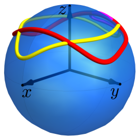
Figure 3: Trajectories on the Bloch sphere of the atoms order parameters as a function of time in steady-state, $f[x(t),y(t),z(t),t]$. The trajectories are for $\epsilon=0.5\Omega$, $\lambda_{0}=0.4\Omega$, and $\kappa=\eta=0.1\Omega$. The trajectory that does not encircle the $z$-axis (magenta) is in SP with $\omega_{0}=0.6\Omega$. The trajectories that encircle the $z$-axis (red and yellow) are for $\omega_{0}=0.65\Omega$ and $\omega_{0}=1.5\Omega$, respectively.

To better understand the nature of the D-NP, as well as the effects of the drive $\epsilon\neq 0$ on the NP and SP, we analyze the oscillatory behaviour around the steady-state mean-field solutions of Eqs. (6)-(8). Typically, we find that each phase has a different oscillatory behavior: (i) in NP, the order parameters converge to zero and do not oscillate, (ii) in SP, the oscillations are small but mildly grow with $\epsilon$, and (iii) in D-NP, the order parameters oscillate strongly around zero sup . We, then, Fast Fourier Transform (FFT) the steady-state solutions for each $\omega_{0}$ and $\epsilon$. In both SP and D-NP regimes, the oscillations have a complex beat structure that corresponds to a comb of peaked frequencies at $\omega\neq 0$, as well as $\omega\neq\Omega,\omega_{0}$ sup . Note that the frequencies that appear can be understood from Floquet analysis Morse and Feshbach (1953). In Figs. 2(b), we plot the amplitude of the largest $\omega\neq 0$ peak in the FFT landscape in order to quantify the overall extent of the oscillation. We find that, SP has weak oscillations in all of the order parameters, whereas the D-NP is strongly oscillatory in the $x-y$ plane. These aspects are better highlighted in Fig. 3, by plotting the steady-state time-dependent trajectory of the total spin $\langle\sum_{i}{\bf s}^{i}|(t)\rangle$ on the Bloch sphere for different parameter values. It appears that a distinguishing criterion between the SP and D-NP is whether the trajectory encircles the $z$-axis. Our results seem to indicate that the most plausible candidate for the D-NP is a ”normal phase” in a dynamical rotating frame.

Combining the results from the normal modes and mean field analyses, we see that periodic modulation of the atom-light coupling results in a rich phase diagram, characterized by a multitude of dynamical phase boundaries between the NP, SP and the intriguing new phase, D-NP. All three phases meet at a multicritical point. In the D-NP, the cavity periodically emits pulses of photons with opposing phases, which should be detectable experimentally. The NP $\rightarrow$ SP boundary is principally dictated by where the normal mode $A_{2}$ becomes unstable, whereas the NP $\rightarrow$ D-NP boundary is fixed by the instability of any of the modes $A_{m}$ sup . Within our mean field approach, we find the transitions SP $\rightarrow$ NP, D-NP to be continuous, though the latter is rather sharp. However, the nature of the NP $\rightarrow$ D-NP transition cannot be studied within our approach. The topography of the phase diagram is expected to vary with the choice of $\lambda_{0}$ and the strength of dissipation. Consequently, though the three phases would exist, the highly sensitive multicritical point may disappear.

Remarkably, we see that dissipation leads to a sizable stabilization of the NP. Due to the parametric nature of the normal modes, the NP in the driven case can manifest a dissipation-assisted generation of substantial entanglement/squeezing between the atoms of the condensate and the cavity Galve et al. (2010). The physical signature of such entanglement as well as the impact of parametric driving and dissipation on the critical exponents defining the different phase transitions merit in-depth studies. It would also be interesting to extend the present work to other parameter regimes like $\omega_{a}<<\omega_{c}$ realized in current experimental setups Brennecke et al. (2013).

Our work shows that parametric driving is a powerful tool in the quest for new physics, which exists exclusively in the realm far from equilibrium. The richness of the physics seen in the simple Dicke model presages intriguing phenomena in time-dependent systems, which requires the development of new theoretical methodologies. This frontier is potentially best explored using experimental light-matter systems.

We would like to thank T. Donner, R. Mottl, R. Landig, T. Esslinger, L. Papariello, and E. van Nieuwenburg for useful discussions. We acknowledge financial support from the Swiss National Science Foundation (SNSF).

SUPPLEMENTAL MATERIAL

I I. Normal Phase

A normal mode with time-dependent frequency modulation [cf. Eq. (4) in the main text] can be generically described by the Hamiltonian for a parametric oscillator:

$$H=\frac{p^{2}}{2m}+\frac{1}{2}[\omega_{0}^{2}+\mu(t)]x^{2}\,.$$ (I.1)

For a classical oscillator with sinusoidal modulation, the above Hamiltonian describes the well known Mathieu parametric oscillator McLachlan (1964); Nayfeh and Mook (1979). The quantum parametric Hamiltonian can be rewritten as

$$H =[\omega_{0}+\frac{\mu(t)}{2\omega_{0}}]a^{\dagger}a+\frac{\mu(t)}{4\omega_{0}}(a^{2}+a^{\dagger 2})$$

$$\equiv\sqrt{\omega^{2}_{0}+\mu(t)}{\bar{a}}^{\dagger}{\bar{a}}\,,$$ (I.2)

where the ladder operators $a,a^{\dagger}$ are defined with respect to the time independent model (i.e., $\mu(t)=0$).

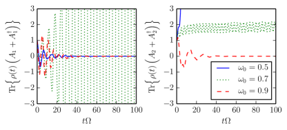
Figure I.1: Characteristic numerical time-integration plots of Eq. (I.8) in different regions of the phase diagram. All curves are with $\lambda_{0}=0.4\Omega$, $\epsilon=0.5\Omega$, and $\kappa=\eta=0.1\Omega$. We see that for (i) $\omega_{0}=0.5\Omega$, mode $A_{1}$ is stable whereas $A_{2}$ is not, (ii) $\omega_{0}=0.7\Omega$, mode $A_{1}$ is unstable whereas $A_{2}$ is stable, and (iii) $\omega_{0}=0.9\Omega$, both modes $A_{m}$ are stable.

We consider a coupling to an external bath which is in the rotating wave approximation. Hence, the solutions to the Heisenberg equations of motion, in the presence of dissipation, for the operators $a$ and $a^{\dagger}$ take the form Tan and Zhang (2011)

$$a(t) = G(t)a(0)+L^{*}(t)a^{\dagger}(0)+F(t)\,,$$ (I.3)

$$a^{\dagger}(t) = G^{*}(t)a^{\dagger}(0)+L(t)a(0)+F^{\dagger}(t)\,,$$ (I.4)

where $G$ and $L$ are time dependent functions obeying the initial conditions $G(0)=G^{*}(0)=1$ and $L(0)=L^{*}(0)=0$. $F$ is an operator term which stems from the dissipation and also depends on the functions $G$ and $L$. It satisfies the condition $F(0)=F^{\dagger}(0)=0$. The functions $G,L$ obey the integro-differential equations

(I.5)

(I.6)

where the dissipative kernel $K(t)=\int d\omega J(\omega)e^{-i\omega t}$ and $J(\omega)$ is the spectral density of the dissipative bath.

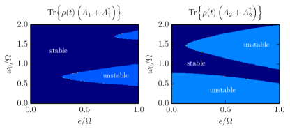
Figure I.2: The numerical stability diagram of the normal modes $A_{m}$ [cf. Eq. (4) in the main text] for $\lambda_{0}=0.4\Omega$ and $\kappa=\eta=0.1\Omega$. As the drive in the Dicke model affects each mode differently, we obtain two “Arnold tongue” stability diagrams that are shifted and scaled with respect to each other. Superposing the zones where both modes are stable leads to the stability of the normal phase (NP) [cf. Fig. 2 in the main text].

These coupled first order integro-differential equations are rather difficult to solve and numerical solutions are needed. However, for standard Markovian dissipation, induced by cavity leakage in the rotating frame or coupling to an ohmic bath, $K(t)=\gamma\delta(t)$ where $\gamma$ is the damping rate. Substituting this in Eqs. (I.5) and (I.6), we see that they become a set of linear ODEs. Observables and correlation functions can easily be obtained from these solutions. For example,

$$\langle a(t)\rangle=G(t)\langle a(0)\rangle+L^{*}(t)\langle a^{\dagger}(0)\rangle+\langle F(t)\rangle\,,$$ (I.7)

where the expectation values are with respect to the initial density matrix. Assuming initial conditions such that $\langle F(t)\rangle=0$, which are expected for baths with no particular ordering, we obtain

$$\langle x(t)\rangle ={\rm Tr}\left\{\rho(t)\left(a+a^{\dagger}\right)\right\}$$ (I.8)

$$={\rm Re}[G(t)+L(t)]\langle x(0)\rangle-{\rm Im}[G(t)+L(t)]\frac{\langle p(0)\rangle}{m\omega_{0}}\,.$$

For arbitrary initial conditions, the stability of the oscillator is dictated by whether the pre-factors $\left[G(t)+L(t)\right]$ grow with time as one approaches the asymptotic state. For the parametric oscillator, we expect it to become exponentially unstable as the strength of the driving is increased Zerbe et al. (1994). Choosing $\mu(t)=g\cos(2\Omega t)$, the zones of stability can be traced in the $\omega_{0}-g$ plane. The resulting stability diagram is the same as that for the classical Mathieu oscillators, which can also be extracted from the classical equations of motions [cf. Eq. (5) in the main text].

To obtain the full NP stability diagram of the Dicke model [see Fig 2 in the main text], we study the stability of both normal modes $A_{m}$, $m=1,2$, with frequencies [cf. Eq. (4) in the main text]

$$\Omega_{1}^{2}(t) = \omega_{0}^{2}+2\lambda_{0}\omega_{0}+2\omega_{0}\epsilon\cos(2\Omega t)\,,$$ (I.9)

$$\Omega_{2}^{2}(t) = \omega_{0}^{2}-2\lambda_{0}\omega_{0}-2\omega_{0}\epsilon\cos(2\Omega t)\,.$$ (I.10)

To simplify our calculation, we also assume that the baths the two modes couple to, have identical spectral densities Galve et al. (2010). Though relaxing this condition would lead to more technical complexity, it should not have any nontrivial physical consequence in the limit of weak dissipation studied here.

We solve the corresponding Eqs. (I.5)-(I.6) and in Fig. I.1, we present characteristic numerical time-integration plots of Eq. (I.8) for the normal modes $A_{m}$. Repeating this procedure for different $\omega_{0}$ and $\epsilon$, and by checking for converging/diverging solutions [cf. Fig. I.1] we find the stability diagram for both modes $A_{m}$, see Fig. I.2. The superposition of the two stability diagrams then yields the stability of the normal phase shown in Fig. 2.

II II. Mean-field analysis

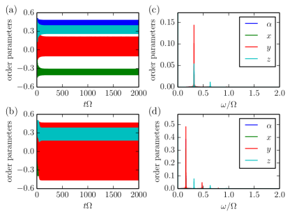
Figure II.1: Characteristic numerical analysis of the mean-field equations [cf. Eqs. (6)-(8) in the main text] leading to the displayed phase diagram [cf. Fig. 2 in the main text]. All plots are with $\lambda_{0}=0.4\Omega$, $\epsilon=0.5\Omega$, and $\kappa=\eta=0.1\Omega$. (a) and (c) are characteristic numerical time-integration plots of the mean-field equations with $\omega_{0}=0.6\Omega$ and $\omega_{0}=0.65\Omega$, respectively. (b) and (d) are the corresponding Fast Fourier Transform (FFT). We see that in the super-radiant phase (SP) region [Figs. (a) and (b)], all order parameters are oscillating around a non-zero mean with relatively small oscillations amplitudes. In the dynamical normal phase (D-NP) region [Figs. (c) and (d)], apart from $z$, all order parameters have a zero mean value, but their oscillations are large taking the full length of the central spin in its $x$ and $y$ components.

In the main text, we obtained a set of coupled non-autonomous mean-field equations [cf. Eqs. (6)-(8) in the main text] for the mean field parameters $\alpha,x~{}{\rm and}~{}y$. These equations were solved numerically with a variety of ODE solvers. Characteristic numerical time-integration plots of the solutions to these equations are shown in Figs. II.1 (a) and (b). Note that the solutions converge to the asymptotic regime for times $t\Omega\sim 500$ and are oscillatory. The time scale for reaching the asymptotic regime varies with the parameters. Repeating this procedure as a function of $\omega_{0}$ and $\epsilon$, the time-average of the order parameters over the steady-state behaviour (the last one-third of the integrated time) is presented in Figs. 2(a) in the main text.

We find that typically the solutions show sinusoidal oscillations characterized by the frequency of the parametric drive. However, in certain parameter regimes, the order parameters oscillate strongly with a complex beat structure involving multiple frequencies. To analyze all these solutions in a systematic manner, we Fast Fourier Transform (FFT) the steady-state signals, see Figs. II.1(c) and (d). The largest amplitude of a finite frequency in such plots serves as a measure for the extent of the oscillation that the order paramaters undergo. This amplitude is plotted as a function of $\omega_{0}$ and $\epsilon$ in Figs. 2(b) in the main text.

References

- Carusotto and Ciuti (2013) I. Carusotto and C. Ciuti, Rev. Mod. Phys. 85, 299 (2013).
- Bloch et al. (2008) I. Bloch, J. Dalibard, and W. Zwerger, Rev. Mod. Phys. 80, 885 (2008).
- Kavokin et al. (2007) A. Kavokin, J. J. Baumberg, G. Malpuech, and F. P. Laussy, Microcavities (Oxford University Press, 2007).
- Wallraff et al. (2004) A. Wallraff, D. I. Schuster, A. Blais, L. Frunzio, R.-S. Huang, J. Majer, S. Kumar, S. M. Girvin, and R. J. Schoelkopf, Nature 431, 162 (2004).
- Majer et al. (2007) J. Majer, J. Chow, J. Gambetta, J. Koch, B. Johnson, J. Schreier, L. Frunzio, D. Schuster, A. Houck, A. Wallraff, et al., Nature 449, 443 (2007).
- Amo et al. (2009) A. Amo, J. Lefrère, S. Pigeon, C. Adrados, C. Ciuti, I. Carusotto, R. Houdré, E. Giacobino, and A. Bramati, Nature Physics 5, 805 (2009).
- Brennecke et al. (2013) F. Brennecke, R. Mottl, K. Baumann, R. Landig, T. Donner, and T. Esslinger, Proceedings of the National Academy of Sciences 110, 11763 (2013).
- Rechtsman et al. (2013) M. C. Rechtsman, J. M. Zeuner, Y. Plotnik, Y. Lumer, D. Podolsky, F. Dreisow, S. Nolte, M. Segev, and A. Szameit, Nature 496, 196 (2013).
- Orzel et al. (2001) C. Orzel, A. Tuchman, M. Fenselau, M. Yasuda, and M. Kasevich, Science 291, 2386 (2001).
- Rugar et al. (2004) D. Rugar, R. Budakian, H. Mamin, and B. Chui, Nature 430, 329 (2004).
- Günter et al. (2009) G. Günter, A. Anappara, J. Hees, A. Sell, G. Biasiol, L. Sorba, S. De Liberato, C. Ciuti, A. Tredicucci, A. Leitenstorfer, et al., Nature 458, 178 (2009).
- Dimer et al. (2007) F. Dimer, B. Estienne, A. S. Parkins, and H. J. Carmichael, Phys. Rev. A 75, 013804 (2007).
- Klinder et al. (2014) J. Klinder, H. Keßler, M. Wolke, L. Mathey, and A. Hemmerich, arXiv preprint arXiv:1409.1945 (2014).
- Nagy et al. (2011) D. Nagy, G. Szirmai, and P. Domokos, Phys. Rev. A 84, 043637 (2011).
- (15) See Supplemental Material for additional details.
- (16) Though in current experimental setups, we explore the impact of larger drive amplitudes as well.
- Bastidas et al. (2012) V. M. Bastidas, C. Emary, B. Regler, and T. Brandes, Phys. Rev. Lett. 108, 043003 (2012).
- Vacanti et al. (2012) G. Vacanti, S. Pugnetti, N. Didier, M. Paternostro, G. M. Palma, R. Fazio, and V. Vedral, Phys. Rev. Lett. 108, 093603 (2012).
- Shirai et al. (2014) T. Shirai, T. Mori, and S. Miyashita, Journal of Physics B: Atomic, Molecular and Optical Physics 47, 025501 (2014).
- Emary and Brandes (2003) C. Emary and T. Brandes, Phys. Rev. E 67, 066203 (2003).
- Galve et al. (2010) F. Galve, L. A. Pachón, and D. Zueco, Phys. Rev. Lett. 105, 180501 (2010).
- McLachlan (1964) N. W. McLachlan, Theory and application of Mathieu functions (Dover, New York, 1964).
- Nayfeh and Mook (1979) A. H. Nayfeh and D. Mook, Nonlinear oscillations (Willey, New York, 1979).
- Zerbe et al. (1994) C. Zerbe, P. Jung, and P. Hänggi, Phys. Rev. E 49, 3626 (1994).
- Zerbe and Hänggi (1995) C. Zerbe and P. Hänggi, Phys. Rev. E 52, 1533 (1995).
- Hepp and Lieb (1973) K. Hepp and E. H. Lieb, Annals of Physics 76, 360 (1973).
- Morse and Feshbach (1953) P. M. Morse and H. Feshbach, Methods of theoretical physics (McGraw-Hill, 1953).
- Tan and Zhang (2011) H.-T. Tan and W.-M. Zhang, Physical Review A 83, 032102 (2011).