On some aspects of isospin breaking in the decay $K^{\pm}\to\pi^{0}\pi^{0}e^{\pm}\stackrel{{{}_{(-)}}}{{\nu_{e}}}$

Abstract

Two aspects of isospin breaking in the decay $K^{\pm}\to\pi^{0}\pi^{0}e^{\pm}\stackrel{{{}_{(-)}}}{{\nu_{e}}}$ are studied and discussed. The first addresses the possible influence of the phenomenological description of the unitarity cusp on the extraction of the normalization of the form factor from data. Using the scalar form factor of the pion as a theoretical laboratory, we find that this determination is robust under variations of the phenomenological parameterizations of the form factor. The second aspect concerns the issue of radiative corrections. We compute the radiative corrections to the total decay rate for $K^{\pm}\to\pi^{0}\pi^{0}e^{\pm}\stackrel{{{}_{(-)}}}{{\nu_{e}}}$ in a setting that allows comparison with the way radiative corrections were handled in the channel $K^{\pm}\to\pi^{+}\pi^{-}e^{\pm}\stackrel{{{}_{(-)}}}{{\nu_{e}}}$. We find that once radiative corrections are included, the normalizations of the form factor as determined experimentally from data in the two decay channels come to a better agreement. The remaining discrepancy can easily be accounted for by other isospin-breaking corrections, mainly those due to the difference between the masses of the up and down quarks.

I INTRODUCTION

The program of analysing $K_{\ell 4}$ decays of the charged kaon conducted by the NA48/2 collaboration at the CERN SPS has so far been very successful. In the $\pi^{+}\pi^{-}$ channel of the electron mode, $\ell=e$ [the decay $K^{\pm}\to\pi^{+}\pi^{-}e^{\pm}\stackrel{{{}_{(-)}}}{{\nu_{e}}}$ will henceforth be refered to as $K^{+-}_{e4}$], it has led, besides a more precise determination of the corresponding branching ratio and hadronic form factors Batley:2012rf , to a very accurate determination of the $\pi\pi$ $S$-wave scattering lengths $a_{0}^{0}$ and $a_{0}^{2}$ Batley:2007zz ; Batley:2010zza , that constitutes a stringent test of the QCD prediction obtained within the framework of chiral perturbation theory Weinberg:1966kf ; Gasser:1983kx ; Colangelo:2000jc ; Colangelo:2001df .

More recently, the results concerning an analysis of the data obtained in the $\pi^{0}\pi^{0}$ channel of the electron mode [the decay $K^{\pm}\to\pi^{0}\pi^{0}e^{\pm}\stackrel{{{}_{(-)}}}{{\nu_{e}}}$ will henceforth be referred to as $K^{00}_{e4}$] have also become available Batley:2014xwa . Although the number of events is lower [$\sim 6.5\cdot 10^{4}$ events in the $K^{00}_{e4}$ mode vs. $\sim 10^{6}$ events for $K^{+-}_{e4}$], this allows for some cross checks at the level of the structure of one of the form factors, that is identical for the two channels in the isospin limit. The normalisation of this common form factor, as measured in the two channels, reads Batley:2012rf ; Batley:2014xwa

$$|V_{us}|f_{s}[K^{+-}_{e4}] = 1.285\pm 0.001_{\rm stat}\pm 0.004_{\rm syst}\pm 0.005_{\rm ext},$$

$$(1+\delta_{EM})|V_{us}|f_{s}[K^{00}_{e4}] = 1.369\pm 0.003_{\rm stat}\pm 0.006_{\rm syst}\pm 0.009_{\rm ext}.$$ (I.1)

Ignoring for the time being the correction factor $\delta_{EM}$ (we will discuss radiative corrections below), the difference of the two values, as compared to the value measured in the $K^{+-}_{e4}$ channel, amounts to 6.5% in relative terms. This might be considered as a small difference, but given the uncertainties, it is, in statistical terms, quite significant. Adding all errors in quadrature this gives

$$(1+\delta_{EM})\frac{f_{s}[K^{00}_{e4}]}{f_{s}[K^{+-}_{e4}]}=1.065\pm 0.010.\\$$ (I.2)

It seems difficult to ascribe a variation of 6.5% to the radiative correction factor $\delta_{EM}$ alone. While in some regions of phase space radiative corrections can reach the $\pm 10$% level, they usually sum up to $\pm 1$% in the decay rate. The radiative corrections to the $K^{+-}_{e4}$ decay mode have been discussed in several places Vesna04 ; Cuplov:2003bj ; Stoffer:2013sfa at one-loop precision in the low-energy expansion. But no comparable study has been done for the $K^{00}_{e4}$ decay mode. There exists an older, less systematic, analysis NuovoCim that covers the corrections due to virtual photon exchanges and real photon emission, which could provide the relevant contributions at a first stage, but its practical use is somewhat limited, since the expressions given there are not always very explicit, and moreover need to be checked. Furthermore, not all radiative corrections occurring in the charged $K_{e4}^{+-}$ channel Vesna04 ; Cuplov:2003bj ; Stoffer:2013sfa have been taken into account in the analysis of the experimental data. These additional radiative corrections could affect $f_{s}[K^{00}_{e4}]$ and $f_{s}[K^{+-}_{e4}]$ in different ways, and make up for another part of the discrepancy.

If $\delta_{EM}$ alone does not explain the discrepancy (I.2), one has to look for other sources of isospin-breaking effects. These can be due to the difference between the up and down quark masses $m_{u}$ and $m_{d}$, conveniently described by the parameter $R$, with $1/R=(m_{d}-m_{u})/(m_{s}-m_{ud})$, where $m_{s}$ is the mass of the strange quark, whereas $m_{ud}$ denotes the average mass of the up and down quarks, $m_{ud}=(m_{u}+m_{d})/2$. For instance, at lowest order in the chiral expansion, one has Vesna04 ; Nehme:2003bz

$$\frac{f_{s}[K^{00}_{e4}]}{f_{s}[K^{+-}_{e4}]}=\left(1+\frac{3}{2R}\right).$$ (I.3)

Barring contributions of higher-order corrections, values of $R$ as small as Aoki:2013ldr $R=35.8(1.9)(1.8)$ can account for about two thirds of the effect in Eq. (I.2).

Finally, there are also isospin breaking effects induced by the mass difference between charged and neutral pions. Most notable from this point of view is the presence of a unitarity cusp Batley:2014xwa in the form factor describing the amplitude of the $K^{00}_{e4}$ mode. The interpretation of this cusp is by now well understood, and as in the case of the $K^{\pm}\to\pi^{0}\pi^{0}\pi^{\pm}$ decay BudiniFonda61 ; Cabibbo:2004gq ; Cabibbo:2005ez ; Gamiz:2006km ; Colangelo:2006va , it arises from the contribution of a $\pi^{+}\pi^{-}$ intermediate state in the unitarity sum [for a general discussion of the properties of the $K_{e4}$ form factors from the point of view of analyticity and unitarity, see Ref. Bernard:2013faa and references therein].

This cusp contains information on the combination $a_{0}^{0}-a_{0}^{2}$ that describes the amplitude for the process $\pi^{+}\pi^{-}\to\pi^{0}\pi^{0}$ at threshold. Although this information probably cannot be extracted from the $K^{00}_{e4}$ data in a way as statistically significant as the determination from the cusp in $K^{\pm}\to\pi^{0}\pi^{0}\pi^{\pm}$ NA48-Kpi3 , it is nevertheless important to include a correct description of this cusp in the parameterisation of the form factor used to analyse the data. This necessity has been demonstrated in full details in the case of the $K^{\pm}\to\pi^{0}\pi^{0}\pi^{\pm}$ decay, and it is to be expected that the same attention to these matters should be paid also in the analysis of the $K^{00}_{e4}$ data. Failure to do so may introduce a systematic bias which would make the comparison with the information on the form factor extracted from the $K^{+-}_{e4}$ data spurious to some extent.

It is the purpose of the present note to address some of these issues. In a first step, we investigate the possible influence that various parameterisations of the form factors could have on the outcome of the analysis. In order to control inputs and ouputs fully, we choose to work with a simplified model, where the exact form factors are known from a theoretical point of view, and where one can assess the effects of various choices of parameterisations for the form factors used in order to analyse the numerically generated data [that we will henceforth refer to as pseudo-data]. This framework is provided by the scalar form factors of the pions, defined as

$$\langle\pi^{0}(p_{1})\pi^{0}(p_{2})|{\widehat{m}}({\overline{u}}u+{\overline{d}}d)(0)|\Omega\rangle = +F_{S}^{\pi^{0}}(s)\quad{}[s\equiv(p_{1}+p_{2})^{2}],$$

$$\langle\pi^{+}(p_{\mbox{\tiny{$+$}}})\pi^{-}(p_{\mbox{\tiny{$-$}}})|{\widehat{m}}({\overline{u}}u+{\overline{d}}d)(0)|\Omega\rangle = -F_{S}^{\pi}(s)\quad{}[s\equiv(p_{\mbox{\tiny{$+$}}}+p_{\mbox{\tiny{$-$}}})^{2}].$$ (I.4)

Expressions of these form factors, with isospin-breaking contributions due to the difference of masses between charged and neutral pions included, have been recently obtained in DescotesGenon:2012gv up to and including two loops in the low-energy expansion. We will use these expressions in order to generate pseudo-data, which we can then submit to analysis, using various parameterisations for the form factors, inspired by those in use for the analyses of the $K^{+-}_{e4}$ and $K^{00}_{e4}$ experimental data. The reason for working with the scalar form factors is at least twofold. First, the form factors, with isospin-breaking effects included, are known at two loops in both channels, whereas in the $K_{e4}$ case, only the form factors in the channel with two charged pions have been studied at the same level of accuracy as far as isospin-breaking corrections are concerned Bernard:2013faa [see Ref. Colangelo:2008sm for a systematic study at one loop]. Second, the $K_{e4}$ form factors depend on two more kinematical variables, besides the di-pion invariant mass. The scalar form factors depend only on the latter, and offer therefore a simple kinematical environment, so that the issues we wish to focus on can be addressed without unnecessary additional complications.

In a second step, we address the issue of radiative corrections to the total decay rate of the decay $K^{\mp}\to\pi^{0}\pi^{0}e^{\mp}\stackrel{{{}_{(-)}}}{{\nu_{e}}}$. Our intent here is not to develop a full one-loop calculation, at the same level of precision as those that exist for the decay channel into two charged pions Vesna04 ; Cuplov:2003bj ; Stoffer:2013sfa . We rather aim at providing a simple estimate for the radiative corrections to the total decay rate, much in the spirit of Refs. NuovoCim and Bystritskiy:2009iv or, on a more general level, of Ref. Isidori:2007zt . This will allow us to assess how much of the discrepancy (I.2) has to be ascribed to other isospin-breaking effects in the form factors, such as discussed above.

The remainder of this study is then organised in the following way. First, we give (Section II) a theoretical discussion of the structure of the scalar form factors of the pions using the explicit expressions obtained in Ref. DescotesGenon:2012gv . We will thus adapt the discussion of Ref. Batley:2014xwa to the case at hand. Working on this analogy will allow us to give an assessment of some additional assumptions regarding the structure of the form factors implicitly made in Ref. Batley:2014xwa . Next, we generate pseudo-data (Section III) using the known two-loop expressions of the form factors, that we then analyze using various phenomenological parameterisations, that do not necessarily comply with the outcome of Section II. The purpose here is to discuss in a quantitative way the possible systematic biases that can be induced by these different choices. The last part of Section III addresses the determination of the combination $a_{0}^{0}-a_{0}^{2}$ of $S$-wave scattering lengths. Radiative corrections, aiming at an estimate of the correction factor $\delta_{EM}$ in Eq. (I.1), are discussed in Section IV. We first compute radiative corrections to the $K_{e4}^{00}$ decay rate in a similar set-up to the one used for the treatment of the data in the $K_{e4}^{+-}$ channel, in order to obtain a meaningful comparison between the two channels. Then we compute the effects of additional photonic corrections, not included in this treatment. Finally, we end our study with a summary and conclusions. Two Appendices contain technical details relevant for the discussions in Section II and in Section IV, respectively.

II Describing the cusp: theory

According to the general analysis of Ref. Cabibbo:2005ez , the occurence of both $\pi^{0}\pi^{0}$ and $\pi^{+}\pi^{-}$ intermediate states at different thresholds leads to the following structure for the scalar form factor of the neutral pion ${F}_{S}^{\pi^{0}}(s)$ [$M_{\pi}$ stands for the charged-pion mass, whereas $M_{\pi^{0}}$ is the mass of the neutral pion]:

$$e^{-i\delta(s)}{F}_{S}^{\pi^{0}}(s)\ =\ \left\{\begin{array}[]{l}{\cal F}_{0}^{\pi^{0}}(s)-i{\cal F}_{1}^{\pi^{0}}(s)\quad[s\geq 4M_{\pi}^{2}]\\ \\ {\cal F}_{0}^{\pi^{0}}(s)+{\cal F}_{1}^{\pi^{0}}(s)\quad\,\,[4M_{\pi^{0}}^{2}\leq s\leq 4M_{\pi}^{2}]\end{array}\right.,$$ (II.4)

where ${\cal F}_{0}^{\pi^{0}}(s)$ is a function of $s$ that is smooth as long as no other threshold, corresponding to higher intermediate states, is reached. Here $\delta(s)$ represents a phase. It can be chosen arbitrarily, as long as it is also a smooth function of $s$. The cusp at $s=4M_{\pi}^{2}$ observed in the differential decay rates corresponding to this simplified [as compared to $K_{e4}$] situation then results from this decomposition, since

$$\left|{F}_{S}^{\pi^{0}}(s)\right|^{2}\ =\ \left\{\begin{array}[]{l}\left|{\cal F}_{0}^{\pi^{0}}(s)\right|^{2}+\left|{\cal F}_{1}^{\pi^{0}}(s)\right|^{2}-2{\rm Im}\,\left[{\cal F}_{0}^{\pi^{0}}(s){\cal F}_{1}^{\pi^{0}*}(s)\right]\quad[s\geq 4M_{\pi}^{2}]\\ \\ \left|{\cal F}_{0}^{\pi^{0}}(s)\right|^{2}+\left|{\cal F}_{1}^{\pi^{0}}(s)\right|^{2}+2{\rm Re}\,\left[{\cal F}_{0}^{\pi^{0}}(s){\cal F}_{1}^{\pi^{0}*}(s)\right]\quad[4M_{\pi^{0}}^{2}\leq s\leq 4M_{\pi}^{2}]\end{array}\right..$$ (II.8)

Apart from the dependence with respect to the second kinematical variable $s_{e}$, the empirical parameterisation used for the fit to the $K_{e4}^{00}$ data, Eq. (9.1) in Ref. Batley:2014xwa , complies with this general representation provided [the variable $S_{\pi}$ used in this reference corresponds to the variable $s$ used here]:

1) ${\cal F}_{1}^{\pi^{0}}(s)$ is parameterised as a real constant times ${\hat{\sigma}}(s)$, with

$${\hat{\sigma}}(s)=\sqrt{\left|1-\frac{4M_{\pi}^{2}}{s}\right|}=\sqrt{\left|\frac{q^{2}}{1+q^{2}}\right|},$$ (II.9)

for $4M_{\pi^{0}}^{2}\leq s\leq 4M_{\pi}^{2}$, or $q^{2}\leq 0$, with $s=4M_{\pi}^{2}(1+q^{2})$.

2) ${\cal F}_{1}^{\pi^{0}}(s)$ is set to zero (its value for $s=4M_{\pi}^{2}$) for $s\geq 4M_{\pi}^{2}$ ($q^{2}\geq 0$)

3) For $4M_{\pi^{0}}^{2}\leq s\leq 4M_{\pi}^{2}$ ($q^{2}\leq 0$), ${\cal F}_{0}^{\pi^{0}}(s)$ is replaced by a constant, equal to ${\cal F}_{0}^{\pi^{0}}(4M_{\pi}^{2})$.

A more theoretically based parameterization, adapted from the simple discussion of the cusp in $K^{\pm}\to\pi^{0}\pi^{0}\pi^{\pm}$ given in Ref. Cabibbo:2004gq , is considered in Sec. 9.4 of Ref. Batley:2014xwa , though not used for the data analysis. As compared to Eq. (II.8), its validity also rests on additional assumptions, which, once transposed to the present situation, read:

1’) The phase $\delta(s)$ can be chosen such as to make the two functions ${\cal F}_{0}^{\pi^{0}}(s)$ and ${\cal F}_{1}^{\pi^{0}}(s)$ simultaneously real, so that Eq. (II.8) takes the simpler form

$$|{F}_{S}^{\pi^{0}}(s)|^{2}\ =\ \left\{\begin{array}[]{l}|{\cal F}_{0}^{\pi^{0}}(s)|^{2}+|{\cal F}_{1}^{\pi^{0}}(s)|^{2}\quad[s\geq 4M_{\pi}^{2}]\\ \\ {}[{\cal F}_{0}^{\pi^{0}}(s)+{\cal F}_{1}^{\pi^{0}}(s)]^{2}\qquad[4M_{\pi^{0}}^{2}\leq s\leq 4M_{\pi}^{2}]\end{array}\right..$$ (II.13)

2’) ${\cal F}_{1}^{\pi^{0}}(s)$ is related to the scalar form factor ${F}_{S}^{\pi}(s)$ of the charged pion, multiplied by a combination of the two $S$-wave $\pi\pi$ scattering lengths $a_{0}^{0}$ and $a_{0}^{2}$ in the isospin limit,

$${\cal F}_{1}^{\pi^{0}}(s)=-\frac{2}{3}\left(a_{0}^{0}-a_{0}^{2}\right){\cal F}_{S}^{\pi}(s){\hat{\sigma}}(s).$$ (II.14)

In view of the discussion in Ref. Batley:2014xwa , ${\cal F}_{S}^{\pi}(s)$ should be identified with the phase-removed scalar form factor of the charged pion. The latter is given by $e^{-i\delta_{0}^{\pi}(s)}F_{S}^{\pi}(s)$, where the phase $\delta_{0}^{\pi}(s)$ is defined as $F_{S}^{\pi}(s+i0)=e^{2i\delta_{0}^{\pi}(s)}F_{S}^{\pi}(s-i0)$.

Our purpose in this Section is twofold. First, we will rewrite the two-loop representation of the form factor ${F}_{S}^{\pi^{0}}(s)$ obtained in Ref. DescotesGenon:2012gv in the form (II.8), that makes the cusp structure explicit. Second, we will assess to which extent the additional features mentioned above and assumed in Ref. Batley:2014xwa are actually reproduced by the structure of the form factors at two loops in the low-energy expansion. In particular, we will establish the precise relation between ${\cal F}_{S}^{\pi}(s)$ and ${F}_{S}^{\pi}(s)$ in Eq. (II.14) at this order. In what follows, and unless otherwise stated, it will always be understood that $s\geq 4M_{\pi^{0}}^{2}$. Furthermore, in practice $s\geq 4M_{\pi}^{2}$ will actually mean $4M_{\pi}^{2}\leq s\leq M_{K}^{2}$, where $M_{K}$ is the mass of the charged kaon, so that we need not worry about thresholds other than those produced by two-pion intermediate states.

II.1 The cusp in the one-loop form factor

We start with the study of the cusp using the one-loop expression of the form factor $F_{S}^{\pi^{0}}(s)$,

$$F_{S}^{\pi^{0}}(s)=F_{S}^{\pi^{0}}\!(0)\!\Bigg{[}1+a_{S}^{\pi^{0}}\!s+16\pi\frac{\varphi_{0}^{00}(s)}{2}{\bar{J}}_{0}(s)\!\Bigg{]}\,-\,16\pi{F_{S}^{\pi}(0)}\,\varphi_{0}^{x}(s)\,{\bar{J}}(s).$$ (II.15)

In this expression, $a_{S}^{\pi^{0}}$ denotes a subtraction constant, that we need not specify further for the time being. The loop functions ${\bar{J}}_{0}(s)$ and ${\bar{J}}(s)$ are given by

$${\bar{J}}_{0}(s) = \frac{s}{16\pi^{2}}\,\int_{4M_{\pi^{0}}^{2}}^{\infty}\,\frac{dx}{x}\,\frac{1}{x-s-i0}\,\sigma_{0}(x)$$

$${\bar{J}}(s) = \frac{s}{16\pi^{2}}\,\int_{4M_{\pi}^{2}}^{\infty}\,\frac{dx}{x}\,\frac{1}{x-s-i0}\,\sigma(x),$$ (II.16)

with

$$\sigma_{0}(s)\,=\,\sqrt{1-\frac{4M_{\pi^{0}}^{2}}{s}}\,,\ \sigma(s)\,=\,\sqrt{1-\frac{4M_{\pi}^{2}}{s}}.$$ (II.17)

The functions $\varphi_{0}^{00}(s)$ and $\varphi_{0}^{x}(s)$ denote the lowest-order real parts of the $S$-wave projections of the amplitudes of the processes $\pi^{0}\pi^{0}\to\pi^{0}\pi^{0}$ and $\pi^{0}\pi^{0}\to\pi^{+}\pi^{-}$, respectively. Their expressions read

$$\varphi_{0}^{00}(s)=a_{00},\quad\varphi_{0}^{x}(s)=a_{x}+b_{x}\frac{s-4M_{\pi}^{2}}{F_{\pi}^{2}},$$ (II.18)

with Knecht:1997jw ; DescotesGenon:2012gv ; Bernard:2013faa

$$a_{00}=\frac{2}{3}\left(a_{0}^{0}+2a_{0}^{2}\right)\left(1-\frac{\Delta_{\pi}}{M_{\pi}^{2}}\right),\ a_{x}=-\frac{2}{3}\left(a_{0}^{0}-a_{0}^{2}\right)+a_{0}^{2}\frac{\Delta_{\pi}}{M_{\pi}^{2}}\,,\ b_{x}=-\frac{1}{12}\left(2a_{0}^{0}-5a_{0}^{2}\right)\frac{F_{\pi}^{2}}{M_{\pi}^{2}},$$ (II.19)

and $\Delta_{\pi}\equiv M_{\pi}^{2}-M_{\pi^{0}}^{2}$.

In the range of $s$ under consideration, the function ${\bar{J}}_{0}(s)$ is complex, but both its real and imaginary parts are smooth,

$${\bar{J}}_{0}(s)=\frac{1}{16\pi^{2}}\left[2+\sigma_{0}(s)L_{0}(s)+i\pi\sigma_{0}(s)\right],\ L_{0}(s)\equiv\ln\left(\frac{1-\sigma_{0}(s)}{1+\sigma_{0}(s)}\right)\qquad[s\geq 4M_{\pi^{0}}^{2}],$$ (II.20)

whereas ${\bar{J}}(s)$ may be rewritten as

$${\bar{J}}(s)\ =\ {\bar{J}}^{[0]}(s)+{\bar{J}}^{[1]}(s)\times\left\{\begin{array}[]{l}\!-i{\hat{\sigma}}(s)\quad[s\geq 4M_{\pi}^{2}]\\ \\ \,+{\hat{\sigma}}(s)\quad[4M_{\pi^{0}}^{2}\leq s\leq 4M_{\pi}^{2}]\end{array}\right..$$ (II.24)

The two functions ${\bar{J}}^{[0]}(s)$ and ${\bar{J}}^{[1]}(s)$ are smooth, and read

$${\bar{J}}^{[0]}(s)=\frac{1}{16\pi^{2}}\left[2+\sigma(s){\hat{L}}(s)\right],\ {\bar{J}}^{[1]}(s)=-\frac{1}{16\pi},$$ (II.25)

where

$${\hat{L}}(s)=\ln\left({\displaystyle\frac{1-\sigma(s)}{1+\sigma(s)}}\right)\quad[s\geq 4M_{\pi^{0}}^{2}].$$ (II.26)

In these expressions, the definition of $\sigma(s)$ has been extended below $s=4M_{\pi}^{2}$ by

$$\sigma(s) = \left\{\begin{array}[]{l}\sqrt{1-{\displaystyle\frac{4M_{\pi}^{2}}{s}}}={\hat{\sigma}}(s)\quad\ \ [s\geq 4M_{\pi}^{2}]\\ \\ i\sqrt{\displaystyle{\frac{4M_{\pi}^{2}}{s}}-1}=i{\hat{\sigma}}(s)\quad[4M_{\pi^{0}}^{2}\leq s\leq 4M_{\pi}^{2}]\end{array}\right..$$ (II.30)

According to Eqs. (II.4) and (II.8), ${\bar{J}}(s)$ exhibits a cusp structure at $s=4M_{\pi}^{2}$. One thus obtains, at this order, the decomposition of the form (II.4) for $F_{S}^{\pi^{0}}(s)$, with

$${\cal F}_{0}^{\pi^{0}}(s) = F_{S}^{\pi^{0}}\!(0)\Bigg{\{}1+a_{S}^{\pi^{0}}\!s+\frac{\varphi_{0}^{00}(s)}{2\pi}\left[2+\sigma_{0}(s)L_{0}(s)\right]\!\Bigg{\}}-{F_{S}^{\pi}(0)}\frac{\varphi_{0}^{x}(s)}{\pi}\left[2+\sigma(s){\hat{L}}(s)\right]\,+\,{\cal O}(E^{6}),$$

$${\cal F}_{1}^{\pi^{0}}(s) = {F_{S}^{\pi}(0)}\varphi_{0}^{x}(s){\hat{\sigma}}(s)\,+\,{\cal O}(E^{6}),$$ (II.31)

provided one factorises the global phase

$$\delta(s)=\frac{1}{2}\,\sigma_{0}(s)\varphi_{0}^{00}(s)\,+\,{\cal O}(E^{4}).$$ (II.32)

Therefore, up to so far unspecified higher order corrections, the one-loop expression of the form factor can be brought into the form (II.4). Both functions ${\cal F}_{0}^{\pi^{0}}(s)$ and ${\cal F}_{1}^{\pi^{0}}(s)/{\hat{\sigma}}(s)$ are real and smooth for $s\geq 4M_{\pi^{0}}^{2}$ at this stage. However, the expression for ${\cal F}_{1}^{\pi^{0}}(s)$ in (II.31) does not quite comply with Eq. (II.14). Whereas at this stage ${\cal F}_{S}^{\pi}(s)$ is equal to the constant ${F_{S}^{\pi}(0)}$, which, at this order, can be identified with the phase-removed form factor, the combination of scattering lengths that occurs in Eq. (II.14) corresponds to $\stackrel{{\scriptstyle{}_{\mbox{\scriptsize{$o$}}}}}{{\varphi}}\stackrel{{\scriptstyle x}}{{{}_{0}}}\!\!(4M_{\pi}^{2})$, where $\stackrel{{\scriptstyle{}_{\mbox{\scriptsize{$o$}}}}}{{\varphi}}\stackrel{{\scriptstyle x}}{{{}_{0}}}\!\!(s)$ is the expression of $\varphi_{0}^{x}(s)$ in the isospin limit. Thus, at this order, the expression (II.14) misses both the dependence with respect to $s$ in $\varphi^{x}_{0}(s)$, and the isospin-breaking corrections in the scattering lengths.

For later reference, we briefly extend the discussion to the scalar form factor of the charged pion. At one loop, it is given by

$$F_{S}^{\pi}(s)=F_{S}^{\pi}(0)\!\Bigg{[}1+a_{S}^{\pi}\,s+16\pi\varphi_{0}^{\mbox{\tiny{$+-$}}}(s){\bar{J}}(s)\Bigg{]}\,-\,16\pi{F_{S}^{\pi^{0}}(0)}\,\frac{1}{2}\,\varphi_{0}^{x}(s)\,{\bar{J}}_{0}(s).$$ (II.33)

Besides the subtraction constant $a_{S}^{\pi}$, that differs from $a_{S}^{\pi^{0}}$ (they become identical in the isospin limit), this expression involves the lowest-order real part of the $S$-wave projection of the amplitude for the scattering process $\pi^{+}\pi^{-}\to\pi^{+}\pi^{-}$,

$$\varphi_{0}^{\mbox{\tiny{$+-$}}}(s)=a_{\mbox{\tiny{$+-$}}}+b_{\mbox{\tiny{$+-$}}}\frac{s-4M_{\pi}^{2}}{F_{\pi}^{2}},$$ (II.34)

where Knecht:1997jw ; DescotesGenon:2012gv ; Bernard:2013faa

$$a_{\mbox{\tiny{$+-$}}}=\frac{1}{3}\left(2a_{0}^{0}+a_{0}^{2}\right)-2a_{0}^{2}\frac{\Delta_{\pi}}{M_{\pi}^{2}},\ b_{\mbox{\tiny{$+-$}}}=\frac{1}{24}\left(2a_{0}^{0}-5a_{0}^{2}\right)\frac{F_{\pi}^{2}}{M_{\pi}^{2}}.$$ (II.35)

After having factorised the global phase

$${\tilde{\delta}}(s)=-\frac{1}{2}\,\sigma_{0}(s)\varphi_{0}^{x}(s)\,\frac{F_{S}^{\pi^{0}}(0)}{F_{S}^{\pi}(0)}\,+\,{\cal O}(E^{4}),$$ (II.36)

one can decompose $F_{S}^{\pi}(s)$ according to Eq. (II.4), with

$${\cal F}_{0}^{\pi}(s) = F_{S}^{\pi}\!(0)\bigg{\{}1+a_{S}^{\pi}\!s+\frac{\varphi_{0}^{\mbox{\tiny{$+-$}}}(s)}{\pi}\left[2+\sigma(s){\hat{L}}(s)\right]\!\bigg{\}}-{F_{S}^{\pi^{0}}(0)}\frac{\varphi_{0}^{x}(s)}{2\pi}\left[2+\sigma_{0}(s)L_{0}(s)\right]\,+\,{\cal O}(E^{6}),$$

$${\cal F}_{1}^{\pi}(s) = -{F_{S}^{\pi}(0)}\varphi_{0}^{\mbox{\tiny{$+-$}}}(s){\hat{\sigma}}(s)\,+\,{\cal O}(E^{6}).$$ (II.37)

Both functions ${\cal F}_{0}^{\pi}(s)$ and ${\cal F}_{1}^{\pi}(s)/{\hat{\sigma}}(s)$ are real and smooth for $s\geq 4M_{\pi^{0}}^{2}$ at this stage.

II.2 The cusp in the two-loop form factor $F_{S}^{\pi^{0}}(s)$ of the neutral pion

Let us now go through the same analysis, but with the two-loop expression of the form factor. The expressions of the pion scalar form factors at two loops and in presence of isospin breaking have been worked out in Ref. DescotesGenon:2012gv using a recursive construction based on general properties like relativistic invariance, unitarity, analyticity, and chiral counting. The scalar form factor of the neutral pion can be written as

$$F_{S}^{\pi^{0}}(s) = F_{S}^{\pi^{0}}\!(0)\!\left(1+a_{S}^{\pi^{0}}\!s+b_{S}^{\pi^{0}}\!s^{2}\right)$$ (II.38)

$$+\,8\pi F_{S}^{\pi^{0}}\!(0)\varphi_{0}^{00}(s)\left[1+a_{S}^{\pi^{0}}\!s+\frac{1}{\pi}\varphi_{0}^{00}(s)\right]\!{\bar{J}}_{0}(s)$$

$$-\,16\pi{F_{S}^{\pi}(0)}\,\varphi_{0}^{x}(s)\left[1+a_{S}^{\pi}\,s+\frac{2}{\pi}\varphi_{0}^{\mbox{\tiny{$+-$}}}(s)\right]\!{\bar{J}}(s)$$

$$+\,\frac{M_{\pi}^{4}}{F_{\pi}^{4}}\,F_{S}^{\pi^{0}}\!(0)\!\left[\xi^{(0)}_{00}(s){\bar{J}}_{0}(s)+\xi^{(1;0)}_{00}(s){\bar{K}}_{1}^{0}(s)+2\xi^{(2;0)}_{00}(s){\bar{K}}_{2}^{0}(s)+\xi^{(3;0)}_{00}(s){\bar{K}}_{3}^{0}(s)\right.$$

$$\left.\qquad\qquad\qquad+\,\xi^{(1;{\mbox{\tiny$\nabla$}})}_{00}(s){\bar{K}}_{1}^{{\mbox{\tiny$\nabla$}}}(s)+\xi^{(3;{\mbox{\tiny$\nabla$}})}_{00}(s){\bar{K}}_{3}^{{\mbox{\tiny$\nabla$}}}(s)+2\xi^{(2;{\mbox{\tiny{$\!\pm$}}})}_{00}(s)\left[16\pi^{2}{\bar{J}}(s)-2\right]{\bar{J}}_{0}(s)\right]$$

$$-\,2\,\frac{M_{\pi}^{4}}{F_{\pi}^{4}}\,F_{S}^{\pi}(0)\left[\xi^{(0)}_{x}(s){\bar{J}}(s)+2\xi^{(2;{\mbox{\tiny{$\!\pm$}}})}_{x}(s){\bar{K}}_{2}(s)+\xi^{(1)}_{x}(s)K_{1}^{x}(s)+\xi^{(3)}_{x}(s)K_{3}^{x}(s)\right.$$

$$\left.\qquad\qquad\qquad+\,2\xi^{(2;0)}_{x}(s)\left[16\pi^{2}{\bar{J}}_{0}(s)-2\right]{\bar{J}}(s)+\Delta_{1}\xi_{x}(s){\bar{\cal K}}^{x}(s)\right]\,+\,{\cal O}(E^{8}).$$

In this formula, the functions $\xi_{00}^{(0)}(s),\ldots,\xi_{x}^{(0)}(s),\ldots$ are polynomials of at most second order in the variable $s$. Their expressions can be found in Ref. DescotesGenon:2012gv , except for $\Delta_{1}\xi_{x}(s)$, that reads

$$\Delta_{1}\xi_{x}(s)=8\,\frac{\Delta_{\pi}}{M_{\pi}^{2}}\,b_{+0}\frac{s}{M_{\pi}^{2}}\left[\frac{s}{9M_{\pi}^{2}}b_{+0}-a_{+0}\frac{F_{\pi}^{2}}{M_{\pi}^{2}}+2b_{+0}\left(1+\frac{M_{\pi^{0}}^{2}}{M_{\pi}^{2}}\right)\right].$$ (II.39)

It is also useful to be aware of the relations

$$\xi^{(2;0)}_{00}(s)=2\frac{F_{\pi}^{4}}{M_{\pi}^{4}}[\varphi_{0}^{00}(s)]^{2}\!,\ \xi^{(2;0)}_{x}(s)=2\frac{F_{\pi}^{4}}{M_{\pi}^{4}}\varphi_{0}^{00}(s)\varphi_{0}^{x}(s),\ \xi^{(2;{\mbox{\tiny{$\!\pm$}}})}_{00}(s)=4\frac{F_{\pi}^{4}}{M_{\pi}^{4}}[\varphi_{0}^{x}(s)]^{2}\!,\ \xi^{(2;{\mbox{\tiny{$\!\pm$}}})}_{x}(s)=4\frac{F_{\pi}^{4}}{M_{\pi}^{4}}\varphi_{0}^{x}(s)\varphi^{\mbox{\tiny{$+-$}}}(s).$$ (II.40)

In order to achieve the decomposition (II.4), we need to extend the decomposition of the function ${\bar{J}}(s)$ in Eqs. (II.24) and (II.25) to the other functions, denoted generically by ${\bar{K}}_{n}^{\alpha}(s)$, that appear in the expression (II.38). This may be done as follows. First, we may observe that, like ${\bar{J}}_{0}(s)$ or ${\bar{J}}(s)$, these functions can also be defined by a dispersive representation of the form [for ${\bar{J}}_{0}(s)\equiv{\bar{K}}_{0}^{0}(s)$, one has $k_{0}^{0}(s)=\sigma_{0}(s)/16\pi$, whereas for ${\bar{J}}(s)\equiv{\bar{K}}_{0}(s)$, $k_{0}(s)=\sigma(s)/16\pi$, see Eq. (II.16)]

$${\bar{K}}_{n}^{\alpha}(s)=\frac{s}{\pi}\,\int_{s_{\rm thr}}^{\infty}\,\frac{dx}{x}\,\frac{1}{x-s-i0}\,k_{n}^{\alpha}(x).$$ (II.41)

Explicit expressions for the functions $k_{n}^{\alpha}(s)$ are given in Appendix A. For the set of functions $K_{n}^{0}(s)$ and ${\bar{K}}_{n}^{{\mbox{\tiny$\nabla$}}}(s)$, one has $s_{\rm thr}=4M_{\pi^{0}}^{2}$. These functions will therefore each develop an imaginary part for $s\geq s_{\rm thr}=4M_{\pi^{0}}$, ${\rm Im}{\bar{K}}_{n}^{\alpha}(s)=k_{n}^{\alpha}(s)\theta(s-4M_{\pi^{0}}^{2})$, while the real part displays a cusp at $s=4M_{\pi^{0}}$, but is smooth for $s\geq 4M_{\pi^{0}}$. The situation is different for the remaining functions, ${\bar{K}}_{n}(s)$, ${\bar{K}}_{n}^{x}(s)$, and ${\bar{\cal K}}^{x}(s)$, for which $s_{\rm thr}=4M_{\pi}^{2}$, so that, in a generic way, they have the following structure

$${\bar{K}}_{n}^{\alpha}(s) = {\rm Re}\,{\bar{K}}_{n}^{\alpha}(s)+\left\{\begin{array}[]{l}ik_{n}^{\alpha}(s)\quad[s\geq 4M_{\pi}^{2}]\\ \\ \ 0\qquad\ \ \,[4M_{\pi^{0}}^{2}\leq s\leq 4M_{\pi}^{2}]\end{array}\right.$$ (II.45)

$$= {\rm Re}\,{\bar{K}}_{n}^{\alpha}(s)+\frac{k_{n}^{\alpha}(s)}{\sigma(s)}\times\left\{\begin{array}[]{l}i{\hat{\sigma}}(s)\quad[s\geq 4M_{\pi}^{2}]\\ \\ \ 0\qquad\ \,[4M_{\pi^{0}}^{2}\leq s\leq 4M_{\pi}^{2}]\end{array}\right..$$ (II.49)

In general, the function ${k_{n}^{\alpha}(s)}/{\sigma(s)}$, although real, is not smooth for the whole range $s\geq 4M_{\pi^{0}}^{2}$, but only for $s\geq 4M_{\pi}^{2}$. Suppose one can find a function ${\hat{k}}_{n}^{\alpha}(s)$ such that it coincides with $k_{n}^{\alpha}(s)$ for $s\geq 4M_{\pi}^{2}$, and such that ${\hat{k}}_{n}^{\alpha}(s)/\sigma(s)$ is real and smooth for all $s\geq 4M_{\pi^{0}}^{2}$. Then one can perform the decomposition

$${\bar{K}}(s)\ =\ {\bar{K}}^{[0]}(s)+{\bar{K}}^{[1]}(s)\times\left\{\begin{array}[]{l}\!-i{\hat{\sigma}}(s)\quad[s\geq 4M_{\pi}^{2}]\\ \\ \,+{\hat{\sigma}}(s)\quad[4M_{\pi^{0}}^{2}\leq s\leq 4M_{\pi}^{2}]\end{array}\right.,$$ (II.53)

in terms of two real and smooth functions ${\bar{K}}^{[0]}(s)$ and ${\bar{K}}^{[1]}(s)$, given by

$${\bar{K}}_{n}^{\alpha[0]}(s)\ =\ \left\{\begin{array}[]{l}{\rm Re}\,{\bar{K}}_{n}^{\alpha}(s)\qquad\ \ \,\qquad[s\geq 4M_{\pi}^{2}]\\ \\ {\rm Re}\,{\bar{K}}_{n}^{\alpha}(s)-i{\hat{k}}_{n}^{\alpha}(s)\quad[4M_{\pi^{0}}^{2}\leq s\leq 4M_{\pi}^{2}]\end{array}\right.,\qquad{\bar{K}}_{n}^{\alpha[1]}(s)\ =\ -\frac{{\hat{k}}_{n}^{\alpha}(s)}{\sigma(s)}.$$ (II.57)

Such a decomposition can indeed be achieved for the various functions considered here, as discussed in detail in App. A. The decomposition (II.4) of the form factor now follows immediately, with

$$e^{i\delta(s)}{\cal F}_{0}^{\pi^{0}}(s) = F_{S}^{\pi^{0}}\!(0)\!\left(1+a_{S}^{\pi^{0}}\!s+b_{S}^{\pi^{0}}\!s^{2}\right)$$ (II.58)

$$+\,8\pi F_{S}^{\pi^{0}}\!(0)\varphi_{0}^{00}(s)\left[1+a_{S}^{\pi^{0}}\!s+\frac{1}{\pi}\varphi_{0}^{00}(s)\right]\!{\bar{J}}_{0}(s)$$

$$-\,16\pi{F_{S}^{\pi}(0)}\,\varphi_{0}^{x}(s)\left[1+a_{S}^{\pi}\,s+\frac{2}{\pi}\varphi_{0}^{\mbox{\tiny{$+-$}}}(s)\right]\!{\bar{J}}^{[0]}(s)$$

$$+\,\frac{M_{\pi}^{4}}{F_{\pi}^{4}}\,F_{S}^{\pi^{0}}\!(0)\!\left[\xi^{(0)}_{00}(s){\bar{J}}_{0}(s)+\xi^{(1;0)}_{00}(s){\bar{K}}_{1}^{0}(s)+\xi^{(1;{\mbox{\tiny$\nabla$}})}_{00}(s){\bar{K}}_{1}^{\mbox{\tiny$\nabla$}}(s)+2\,\xi^{(2;0)}_{00}(s){\bar{K}}_{2}^{0}(s)\right.$$

$$\left.\quad\qquad\qquad+\,\xi^{(3;0)}_{00}(s){\bar{K}}_{3}^{0}(s)+\xi^{(3;{\mbox{\tiny$\nabla$}})}_{00}(s){\bar{K}}_{3}^{\mbox{\tiny$\nabla$}}(s)+2\xi^{(2;{\mbox{\tiny{$\pm$}}})}_{00}(s)\left[16\pi^{2}{\bar{J}}^{[0]}(s)-2\right]{\bar{J}}_{0}(s)\right]$$

$$-\,2\,\frac{M_{\pi}^{4}}{F_{\pi}^{4}}\,F_{S}^{\pi}(0)\left[\xi^{(0)}_{x}(s){\bar{J}}^{[0]}(s)+\xi^{(1)}_{x}(s){\bar{K}}_{1}^{x[0]}(s)+2\xi^{(2;{\mbox{\tiny{$\pm$}}})}_{x}(s){\bar{K}}_{2}^{[0]}(s)+\xi^{(3)}_{x}(s){\bar{K}}_{3}^{x[0]}(s)\right.$$

$$\left.\quad\qquad\qquad+\,2\xi^{(2;0)}_{x}(s)\left[16\pi^{2}{\bar{J}}_{0}(s)-2\right]{\bar{J}}^{[0]}(s)+\Delta_{1}\xi_{x}(s){\bar{\cal K}}^{x[0]}(s)\right]\,+\,{\cal O}(E^{8}),$$

and

$$e^{i\delta(s)}{\cal F}_{1}^{\pi^{0}}(s) = -{\hat{\sigma}}(s)\bigg{\{}16\pi{F_{S}^{\pi}(0)}\,\varphi_{0}^{x}(s)\left[1+a_{S}^{\pi}\,s+\frac{2}{\pi}\varphi_{0}^{\mbox{\tiny{$+-$}}}(s)\right]\!{\bar{J}}^{[1]}(s)$$ (II.59)

$$-\,2\,\frac{M_{\pi}^{4}}{F_{\pi}^{4}}\,F_{S}^{\pi^{0}}\!(0)\xi^{(2;{\mbox{\tiny{$\!\pm$}}})}_{00}(s)\times 16\pi^{2}{\bar{J}}_{0}(s){\bar{J}}^{[1]}(s)$$

$$+\,2\,\frac{M_{\pi}^{4}}{F_{\pi}^{4}}\,F_{S}^{\pi}(0)\left[\xi^{(0)}_{x}(s){\bar{J}}^{[1]}(s)+\xi^{(1)}_{x}(s){\bar{K}}_{1}^{x[1]}(s)+2\xi^{(2;{\mbox{\tiny{$\!\pm$}}})}_{x}(s){\bar{K}}_{2}^{[1]}(s)+\xi^{(3)}_{x}(s){\bar{K}}_{3}^{x[1]}(s)\right.$$

$$\left.\quad\qquad\qquad+\,2\xi^{(2;0)}_{x}(s)\left[16\pi^{2}{\bar{J}}_{0}(s)-2\right]{\bar{J}}^{[1]}(s)+\Delta_{1}\xi_{x}(s){\bar{\cal K}}^{x[1]}(s)\right]\bigg{\}}\,+\,{\cal O}(E^{8}).$$

Both functions $e^{i\delta(s)}{\cal F}_{0}^{\pi^{0}}(s)$ and $e^{i\delta(s)}{\cal F}_{1}^{\pi^{0}}(s)/{\hat{\sigma}}(s)$ are smooth for $s\geq 4M_{\pi^{0}}^{2}$, but complex. It remains to discuss the phase $\delta(s)$. If we want to make the function ${\cal F}_{0}^{\pi^{0}}(s)$ real, while keeping it smooth, then its choice is unique,

$$\delta(s)\equiv\frac{1}{2}\,\sigma_{0}(s)\left[\varphi_{0}^{00}(s)+{\hat{\psi}}_{0}^{00}(s)\right],$$ (II.60)

with ${\hat{\psi}}_{0}^{00}(s)$ given by

$$\frac{1}{2}\,\sigma_{0}(s){\hat{\psi}}_{0}^{00}(s) = \frac{M_{\pi}^{4}}{F_{\pi}^{4}}\bigg{[}\xi^{(0)}_{00}(s)k_{0}^{0}(s)+\xi^{(1;0)}_{00}(s)k_{1}^{0}(s)+\xi^{(1;{\mbox{\tiny$\nabla$}})}_{00}(s)k_{1}^{\mbox{\tiny$\nabla$}}(s)+\xi^{(2;0)}_{00}(s)k_{2}^{0}(s)$$ (II.61)

$$\qquad+\xi^{(3;0)}_{00}(s)k_{3}^{0}(s)+\xi^{(3;{\mbox{\tiny$\nabla$}})}_{00}(s)k_{3}^{\mbox{\tiny$\nabla$}}(s)+\xi^{(2;\pm)}_{00}(s)\,\frac{1}{8\pi}\sigma_{0}(s)\sigma(s){\hat{L}}(s)\bigg{]}.$$

Note that ${\hat{\psi}}_{0}^{00}(s)$ differs from the quantity ${\psi}_{0}^{00}(s)$ defined in Eq. (4.6) of Ref. DescotesGenon:2012gv by the presence of the function ${\hat{L}}(s)$ instead of $L(s)$ in the last term between square brackets, see Eq. (A.61). This makes $\sigma_{0}(s){\hat{\psi}}_{0}^{00}(s)$ a smooth function for $s\geq 4M_{\pi^{0}}^{2}$, whereas $\sigma(s)L(s)$, and hence ${\psi}_{0}^{00}(s)$, displays a cusp at $s=4M_{\pi}^{2}$. Making use of Eq. (II.49), the removal of the phase $\delta(s)$ indeed leads to a real and smooth expression for the function ${\cal F}_{0}^{\pi^{0}}(s)$:

$${\cal F}_{0}^{\pi^{0}}(s) = F_{S}^{\pi^{0}}\!(0)\!\left(1+a_{S}^{\pi^{0}}\!s+b_{S}^{\pi^{0}}\!s^{2}\right)$$ (II.62)

$$+\,8\pi F_{S}^{\pi^{0}}\!(0)\varphi_{0}^{00}(s)\left[1+a_{S}^{\pi^{0}}\!s\right]{\rm Re}\,{\bar{J}}_{0}(s)$$

$$-\,16\pi{F_{S}^{\pi}(0)}\,\varphi_{0}^{x}(s)\left[1+a_{S}^{\pi}\,s+\frac{2}{\pi}\varphi_{0}^{\mbox{\tiny{$+-$}}}(s)\right]\!{\bar{J}}^{[0]}(s)$$

$$+\,\frac{M_{\pi}^{4}}{F_{\pi}^{4}}\,F_{S}^{\pi^{0}}\!(0)\!\left[\xi^{(0)}_{00}(s){\rm Re}\,{\bar{J}}_{0}(s)+\xi^{(1;0)}_{00}(s){\rm Re}\,{\bar{K}}_{1}^{0}(s)+\xi^{(1;{\mbox{\tiny$\nabla$}})}_{00}(s){\rm Re}\,{\bar{K}}_{1}^{\mbox{\tiny$\nabla$}}(s)+\right.$$

$$\left.\quad\qquad\qquad+\,\xi^{(2;0)}_{00}(s){\rm Re}\,{\bar{K}}_{2}^{0}(s)+\xi^{(3;0)}_{00}(s){\rm Re}\,{\bar{K}}_{3}^{0}(s)+\xi^{(3;{\mbox{\tiny$\nabla$}})}_{00}(s){\rm Re}\,{\bar{K}}_{3}^{\mbox{\tiny$\nabla$}}(s)\right]$$

$$-\,2\,\frac{M_{\pi}^{4}}{F_{\pi}^{4}}\,F_{S}^{\pi}(0)\left[\xi^{(0)}_{x}(s){\bar{J}}^{[0]}(s)+\xi^{(1)}_{x}(s){\bar{K}}_{1}^{x[0]}(s)+2\xi^{(2;{\mbox{\tiny{$\!\pm$}}})}_{x}(s){\bar{K}}_{2}^{[0]}(s)\right.$$

$$\left.\quad\qquad\qquad+\,\xi^{(3)}_{x}(s){\bar{K}}_{3}^{x[0]}(s)+\Delta_{1}\xi_{x}(s){\bar{\cal K}}^{x[0]}(s)\right]$$

$$+\,8F_{S}^{\pi^{0}}\!(0)\left[\varphi_{0}^{x}(s)\right]^{2}\left(16\pi^{2}{\bar{J}}^{[0]}(s)-2\right){\rm Re}\,{\bar{J}}_{0}(s)$$

$$-\,8F_{S}^{\pi}(0)\varphi_{0}^{x}(s)\varphi_{0}^{00}(s)\left[16\pi^{2}{\rm Re}\,{\bar{J}}_{0}(s)-2\right]{\bar{J}}^{[0]}(s)$$

$$+\,F_{S}^{\pi^{0}}\!(0)\left[\varphi_{0}^{00}(s)\right]^{2}\left[2{\rm Re}\,{\bar{K}}_{2}^{0}(s)+8{\rm Re}\,{\bar{J}}_{0}(s)+\frac{1}{8}\left(1-\frac{4M_{\pi^{0}}^{2}}{s}\right)\right]\,+\,{\cal O}(E^{8}).$$

As far as ${\cal F}_{1}^{\pi^{0}}(s)$ is concerned, we may even proceed in a more direct way by noticing that, up to higher order corrections, Eq. (II.59) rewrites as

$$e^{i\delta(s)}{\cal F}_{1}^{\pi^{0}}(s) = e^{\frac{i}{2}\sigma_{0}(s)\varphi_{0}^{00}(s)}{\hat{\sigma}}(s)\left[\varphi_{0}^{x}(s)+{\hat{\psi}}_{0}^{x}(s)\right]$$ (II.63)

$$\times{F_{S}^{\pi}(0)}\bigg{\{}1+a_{S}^{\pi}s+16\pi\varphi_{0}^{{\mbox{\tiny{$+-$}}}}(s){\bar{J}}^{[0]}(s)-8\pi\frac{F_{S}^{\pi^{0}}(0)}{F_{S}^{\pi}(0)}\,\varphi_{0}^{x}(s){\bar{J}}_{0}(s)\!\bigg{\}}\,+\,{\cal O}(E^{8}),$$

with [for the notation, see Appendix A]

$${\hat{\psi}}_{0}^{x}(s) = 2\,\frac{M_{\pi}^{4}}{F_{\pi}^{4}}\,\frac{1}{\sigma(s)}\,\Bigg{\{}\xi^{(0)}_{x}(s)k_{0}(s)+\xi^{(2;{\mbox{\tiny{$\!\pm$}}})}_{x}(s){\hat{k}}_{2}(s)+\xi^{(1)}_{x}(s)k_{1}^{x}(s)+\xi^{(3)}_{x}(s)k_{3}^{x}(s)$$ (II.64)

$$\qquad\qquad\qquad+\,\xi^{(2;0)}_{x}(s)k_{2}^{x}(s)+\Delta_{1}\xi_{x}(s)k^{x}(s)\Bigg{\}}.$$

Now, the phase that appears factored out on the right-hand side of this equation can be identified with the phase $\delta(s)$ on the left-hand side, since the difference generates contributions of order ${\cal O}(E^{8})$, that are neglected anyway. Taking into account Eqs. (II.36) and (II.37), one finally obtains

$${\cal F}_{1}^{\pi^{0}}(s)={\hat{\sigma}}(s)\left[\varphi_{0}^{x}(s)+{\hat{\psi}}_{0}^{x}(s)\right]{\cal F}_{\pi}(s)\,+\,{\cal O}(E^{8}),$$ (II.65)

with

$${\cal F}_{\pi}(s)\equiv e^{i{\tilde{\delta}}(s)}{\cal F}^{\pi}_{0}(s)\,+\,{\cal O}(E^{6}).$$ (II.66)

It is possible to give a more precise interpretation of the combination $\varphi_{0}^{x}(s)+{\hat{\psi}}_{0}^{x}(s)$ that occurs in (II.65). To this end, let us recall from Ref. DescotesGenon:2012gv that the $\ell=0$ partial-wave projection $f_{0}^{x}(s)$ for the scattering amplitude of the process $\pi^{0}\pi^{0}\to\pi^{+}\pi^{-}$ is given, at order one loop and for $s\geq 4M_{\pi^{0}}^{2}$, by

$$f_{0}^{x}(s)=\varphi_{0}^{x}(s)+{\psi}_{0}^{x}(s)+i\varphi^{x}_{0}(s)\left[\frac{1}{2}\sigma_{0}(s)\varphi_{0}^{00}(s)+\sigma(s)\varphi_{0}^{{\mbox{\tiny{$+-$}}}}(s)\theta(s-4M_{\pi}^{2})\right]\,+\,{\cal O}(E^{6}),$$ (II.67)

where ${\psi}_{0}^{x}(s)$ is defined in Eq. (4.15) of Ref. DescotesGenon:2012gv [the contribution $\Delta_{2}\psi_{0}^{x}(s)$, of second order in isospin breaking, is numerically quite small, and is omitted for simplicity]. It differs from ${\hat{\psi}}_{0}^{x}(s)$ by the replacement of ${\hat{k}}_{2}(s)$ by $k_{2}(s)$ in Eq. (II.64). Then applying the decomposition (II.53) to $f_{0}^{x}(s)$, one finds

$$e^{-i\delta(s)}{f_{0}^{x}}(s)\ =\ {f_{0}^{x}}^{[0]}(s)+{f_{0}^{x}}^{[1]}(s)\times\left\{\begin{array}[]{l}\!-i{\hat{\sigma}}(s)\quad[s\geq 4M_{\pi}^{2}]\\ \\ \,+{\hat{\sigma}}(s)\quad[4M_{\pi^{0}}^{2}\leq s\leq 4M_{\pi}^{2}]\end{array}\right.,$$ (II.71)

with ${f_{0}^{x}}^{[0]}(s)=\varphi_{0}^{x}(s)+{\hat{\psi}}_{0}^{x}(s)+{\cal O}(E^{6})$, and ${f_{0}^{x}}^{[1]}(s)=-\varphi_{0}^{x}(s)\varphi_{0}^{{\mbox{\tiny{$+-$}}}}(s)+{\cal O}(E^{6})$.

We may summarise this theoretical study of the cusp in the scalar form factor of the neutral pion with a couple of remarks:

• It is, in general, not possible to chose the phase $\delta(s)$ in Eq. (II.4) such as to make both ${\cal F}_{0}^{\pi^{0}}(s)$ and ${\cal F}_{1}^{\pi^{0}}(s)$ real simultaneously. A relative phase remains, see Eqs. (II.65) and (II.66). At lowest order, this phase is given by the $S$-wave projection of the inelastic rescattering of a pair of neutral pions through a pair of charged pions, cf. Eq. (II.36).

• The structure of ${\cal F}_{1}^{\pi^{0}}(s)$ is more complicated than just the product of the scattering length corresponding to this rescattering amplitude times the phase removed scalar form factor of the charged pion. At the order we have been working, it involves the decomposition (II.71) of the $S$-wave projection of this amplitude times the part ${\cal F}^{\pi}_{0}(s)$ of the decomposition (II.4) of $F_{S}^{\pi}(s)$. This is different from the phase-removed form factor, as already seen at order one loop:

  $$e^{-i\delta_{0}^{\pi}(s)}F_{S}^{\pi}(s)-{\cal F}^{\pi}_{0}(s)={\cal F}^{\pi}_{1}(s)\times\left\{\begin{array}[]{l}0\quad[s\geq 4M_{\pi}^{2}]\\ \\ 1\quad[4M_{\pi^{0}}^{2}\leq s\leq 4M_{\pi}^{2}]\end{array}\right.\,+\,{\cal O}(E^{6}).$$ (II.72)

  Note however that this difference only concerns the region $4M_{\pi^{0}}^{2}\leq s\leq 4M_{\pi}^{2}$, which contributes very little to the total decay rate as defined by Eqs. (III.1) and (III.2) below.

II.3 Description of the two-loop form factor $F_{S}^{\pi}(s)$ of the charged pion

We now briefly address the scalar form factor of the charged pion. The issue here is not to describe the cusp, that occurs below the physical threshold at $s=4M_{\pi}^{2}$, but to provide the expressions that will be used in the sequel. Again, we will rely on the results obtained in Ref. DescotesGenon:2012gv , and rewrite the form factor $F_{S}^{\pi}(s)$ at two loops in a way that is adapted to our purposes. In particular, we will consider the phase-removed form factor, which reads, in the relevant domain $s\geq 4M_{\pi}^{2}$,

$$e^{-i\delta_{0}^{\pi}(s)}F_{S}^{\pi}(s) = F_{S}^{\pi}\!(0)\!\left(1+a_{S}^{\pi}s+b_{S}^{\pi}s^{2}\right)$$ (II.73)

$$\!\!\!\!\!-\,8\pi F_{S}^{\pi^{0}}\!(0)\varphi_{0}^{x}(s)\left[1+a_{S}^{\pi^{0}}\!s+\frac{1}{\pi}\varphi_{0}^{00}(s)\right]\!{\rm Re}\,{\bar{J}}_{0}(s)$$

$$\!\!\!\!\!+\,16\pi{F_{S}^{\pi}(0)}\,\varphi_{0}^{{\mbox{\tiny{$+-$}}}}(s)\left[1+a_{S}^{\pi}\,s+\frac{2}{\pi}\varphi_{0}^{\mbox{\tiny{$+-$}}}(s)\right]\!{\rm Re}\,{\bar{J}}(s)$$

$$\!\!\!\!\!-\,\frac{M_{\pi}^{4}}{F_{\pi}^{4}}\,F_{S}^{\pi^{0}}\!(0)\!\left\{\xi^{(0)}_{x}(s){\rm Re}\,{\bar{J}}_{0}(s)+\xi^{(1)}_{x}(s){\rm Re}\,{\bar{K}}_{1}^{x_{0}}(s)+2\xi^{(2;0)}_{x}(s){\rm Re}\,{\bar{K}}_{2}^{0}(s)+\xi^{(3)}_{x}(s){\rm Re}\,{\bar{K}}_{3}^{x_{0}}(s)\right.$$

$$\!\!\!\!\!\left.\qquad\qquad\qquad+\,\Delta_{1}\xi_{x}(s){\rm Re}\,{\bar{\cal K}}^{x_{0}}(s)+2\xi^{(2;{\mbox{\tiny{$\!\pm$}}})}_{x}(s)\left[16\pi^{2}{\rm Re}\,{\bar{J}}(s)-2\right]{\rm Re}\,{\bar{J}}_{0}(s)\right\}$$

$$\!\!\!\!\!+\,2\,\frac{M_{\pi}^{4}}{F_{\pi}^{4}}\,F_{S}^{\pi}(0)\left\{\xi_{{\mbox{\tiny{$+-$}}};S}^{(0)}(s){\rm Re}\,{\bar{J}}(s)+\xi^{(1;{\mbox{\tiny{$\pm$}}})}_{{\mbox{\tiny{$+-$}}};S}(s){\rm Re}\,{\bar{K}}_{1}(s)+2\xi^{(2;{\mbox{\tiny{$\pm$}}})}_{{\mbox{\tiny{$+-$}}};S}(s)\left[{\rm Re}\,{\bar{K}}_{2}(s)+\frac{1}{32}\left(1-\frac{4M_{\pi}^{2}}{s}\right)\right]\right.$$

$$\!\!\!\!\!\left.\qquad\qquad\qquad+\,\xi^{(3;{\mbox{\tiny{$\pm$}}})}_{{\mbox{\tiny{$+-$}}};S}(s){\rm Re}\,{\bar{K}}_{3}(s)+\xi^{(1;{\mbox{\tiny$\Delta$}})}_{{\mbox{\tiny{$+-$}}};S}(s){\rm Re}\,{\bar{K}}_{1}^{\mbox{\tiny$\Delta$}}(s)+\xi^{(3;{\mbox{\tiny$\Delta$}})}_{{\mbox{\tiny{$+-$}}};S}(s){\rm Re}\,{\bar{K}}_{3}^{\mbox{\tiny$\Delta$}}(s)+\right.$$

$$\!\!\!\!\!\left.\qquad\qquad\qquad+\,2\xi^{(2;0)}_{{\mbox{\tiny{$+-$}}};S}(s)\left[\left(16\pi^{2}{\rm Re}\,{\bar{J}}_{0}(s)-2\right){\rm Re}\,{\bar{J}}(s)+\frac{1}{64}\left(1-\frac{4M_{\pi^{0}}^{2}}{s}\right)\right]\right\}\,+\,{\cal O}(E^{8}).$$

The functions ${\bar{K}}_{n}^{\alpha}(s)$ that appear in this expression have again a dispersive representation of the form displayed in Eq. (II.41). The absorptive parts are in part given in Appendix A. For the remaining one, we have

$$k_{n}^{x_{0}}(s)=\frac{\sigma_{0}(s)}{\sigma(s)}\,k_{n}^{x}(s),\quad k^{x_{0}}(s)=\frac{\sigma_{0}(s)}{\sigma(s)}\,k^{x}(s),$$ (II.74)

for the functions corresponding to $s_{\rm thr}=4M_{\pi^{0}}^{2}$, and, for those whose dispersive integrals start at $s_{\rm thr}=4M_{\pi}^{2}$,

$$k_{1}^{{\mbox{\tiny$\Delta$}}}(s)\,=\,\frac{1}{8\pi}\,\frac{\sigma(s)}{\sigma_{0}(s-4\Delta_{\pi})}\,L_{0}(s-4\Delta_{\pi})\,,\qquad k_{3}^{{\mbox{\tiny$\Delta$}}}(s)\,=\,\frac{3}{16\pi}\,\frac{M_{\pi^{0}}^{2}}{s\sigma(s)}\,L_{0}^{2}(s-4\Delta_{\pi})\,,$$ (II.75)

with the definitions of the functions $\sigma(s)$, $\sigma_{0}(s)$ and $L_{0}(s)$ for $s\geq 4M_{\pi^{0}}^{2}$ given in Eqs. (II.17), (II.20), and (II.30).

III Generation and analysis of the pseudo-data

In order to study the effect that particular choices of phenomenological parameterisations of the form factors can have on the output, we will first generate numerical data sets for the scalar form factors of the neutral and charged pions. The pseudo-data in question consist of the (unnormalized) decay distribution defined by

$$\frac{d^{2}\Gamma^{\pi^{0}}(s,s_{\ell})}{dsds_{\ell}}\equiv\frac{1}{2}\sqrt{1-\frac{4M_{\pi^{0}}^{2}}{s}}|F_{S;{\mbox{\scriptsize{data}}}}^{\pi^{0}}(s)|^{2}\lambda^{3/2}(M_{K}^{2},s,s_{\ell}),$$ (III.1)

with $\lambda(x,y,z)=x^{2}+y^{2}+z^{2}-2xy-2xz-2yz$. The total decay rate is obtained by integrating the distributions (III.1), convoluted with the $K_{\ell 4}$ phase space, over the whole physical range [we now consider the electron mode only, and set $m_{e}=0$]:

$$\Gamma^{\pi^{0}}={\cal N}\int_{4M_{\pi^{0}}^{2}}^{M_{K}^{2}}ds\int_{0}^{(M_{K}^{2}-\sqrt{s})^{2}}\!\!\!\!\!\!\!ds_{e}\,\frac{d^{2}\Gamma^{\pi^{0}}(s,s_{e})}{dsds_{e}}.$$ (III.2)

Since we consider the scalar form factor instead of $K_{\ell 4}$ form factors, the integration with respect to $s_{\ell}$ involves the phase space only. The overall normalisation factor has been chosen to be the one of the $K_{e4}$ decay,

$${\cal N}=\frac{G_{\rm F}^{2}|V_{us}|^{2}}{3\cdot 2^{12}\pi^{5}M_{K}^{5}}\frac{1}{|F^{\pi}_{S}(0)|^{2}},$$ (III.3)

up to the factor $1/{|F^{\pi}_{S}(0)|^{2}}$, introduced for convenience.

III.1 Form factors and input parameters used for the generation of pseudo-data

The form factors involved in the preceding expressions are considered as known exactly and are constructed as follows. For $F_{S;{\mbox{\scriptsize{data}}}}^{\pi^{0}}(s)$, we will basically use the decomposition of Eq. (II.4), with ${\cal F}_{0}^{\pi^{0}}(s)$ given by Eq. (II.62), and ${\cal F}_{1}^{\pi^{0}}(s)$ given by Eqs. (II.65) and (II.66). Unfortunately, for some of the functions involved in Eq. (II.62), like ${\rm Re}\,{\bar{K}}_{n}^{\mbox{\tiny$\nabla$}}(s)$ or ${\rm Re}\,{\bar{K}}_{n}^{x}(s)$, explicit analytical expressions are not known. For a numerical approach, we could use their dispersive representation, as given by Eq. (II.41). We have however found it more convenient to start from expressions upon which we have full analytical control. For that purpose, one may replace the functions ${\rm Re}\,{\bar{K}}_{n}^{\mbox{\tiny$\nabla$}}(s)$ by the corresponding functions ${\rm Re}\,{\bar{K}}_{n}^{0}(s)$, and likewise ${\rm Re}\,{\bar{K}}_{n}^{x}(s)$ by ${\rm Re}\,{\bar{K}}_{n}(s)$. We also drop the contribution proportional to $\Delta_{1}\xi_{x}(s)$. In the range of $s$ we are interested in, $4M_{\pi^{0}}^{2}\leq s\leq M_{K}^{2}$, the difference induced in ${\cal F}_{0}^{\pi^{0}}(s)$ by these changes is numerically very small. For the scalar form factor of the neutral pion, the resulting expression then reads

$${F}_{S;{\mbox{\scriptsize{data}}}}^{\pi^{0}}(s)\ =\ \left\{\begin{array}[]{l}{\cal F}_{0;{\mbox{\scriptsize{data}}}}^{\pi^{0}}(s)-i{\cal F}_{1;{\mbox{\scriptsize{data}}}}^{\pi^{0}}(s)\quad[s\geq 4M_{\pi}^{2}]\\ \\ {\cal F}_{0;{\mbox{\scriptsize{data}}}}^{\pi^{0}}(s)+{\cal F}_{1;{\mbox{\scriptsize{data}}}}^{\pi^{0}}(s)\quad\,\,[4M_{\pi^{0}}^{2}\leq s\leq 4M_{\pi}^{2}]\end{array}\right.,$$ (III.7)

with

$${\cal F}_{0;{\mbox{\scriptsize{data}}}}^{\pi^{0}}(s) = F_{S}^{\pi^{0}}\!(0)\!\left(1+a_{S}^{\pi^{0}}\!s+b_{S}^{\pi^{0}}\!s^{2}\right)$$ (III.8)

$$+\,8\pi F_{S}^{\pi^{0}}\!(0)\varphi_{0}^{00}(s)\left[1+a_{S}^{\pi^{0}}\!s\right]{\rm Re}\,{\bar{J}}_{0}(s)$$

$$-\,16\pi{F_{S}^{\pi}(0)}\,\varphi_{0}^{x}(s)\left[1+a_{S}^{\pi}\,s+\frac{2}{\pi}\varphi_{0}^{\mbox{\tiny{$+-$}}}(s)\right]\!{\bar{J}}^{[0]}(s)$$

$$+\,\frac{M_{\pi}^{4}}{F_{\pi}^{4}}\,F_{S}^{\pi^{0}}\!(0)\!\left\{\xi^{(0)}_{00}(s){\rm Re}\,{\bar{J}}_{0}(s)+\left[\xi^{(1;0)}_{00}(s)+\xi^{(1;{\mbox{\tiny$\nabla$}})}_{00}(s)\right]{\rm Re}\,{\bar{K}}_{1}^{0}(s)+\right.$$

$$\left.\quad\qquad\qquad+\,\xi^{(2;0)}_{00}(s){\rm Re}\,{\bar{K}}_{2}^{0}(s)+\left[\xi^{(3;0)}_{00}(s)+\xi^{(3;{\mbox{\tiny$\nabla$}})}_{00}(s)\right]{\rm Re}\,{\bar{K}}_{3}^{0}(s)\right\}$$

$$-\,2\,\frac{M_{\pi}^{4}}{F_{\pi}^{4}}\,F_{S}^{\pi}(0)\left[\xi^{(0)}_{x}(s){\bar{J}}^{[0]}(s)+\xi^{(1)}_{x}(s){\bar{K}}_{1}^{[0]}(s)+2\xi^{(2;{\mbox{\tiny{$\!\pm$}}})}_{x}(s){\bar{K}}_{2}^{[0]}(s)+\xi^{(3)}_{x}(s){\bar{K}}_{3}^{[0]}(s)\right]$$

$$+\,8F_{S}^{\pi^{0}}\!(0)\left[\varphi_{0}^{x}(s)\right]^{2}\left(16\pi^{2}{\bar{J}}^{[0]}(s)-2\right){\rm Re}\,{\bar{J}}_{0}(s)$$

$$-\,8F_{S}^{\pi}(0)\varphi_{0}^{x}(s)\varphi_{0}^{00}(s)\left[16\pi^{2}{\rm Re}\,{\bar{J}}_{0}(s)-2\right]{\bar{J}}^{[0]}(s)$$

$$+\,F_{S}^{\pi^{0}}\!(0)\left[\varphi_{0}^{00}(s)\right]^{2}\left[2{\rm Re}\,{\bar{K}}_{2}^{0}(s)+8{\rm Re}\,{\bar{J}}_{0}(s)+\frac{1}{8}\left(1-\frac{4M_{\pi^{0}}^{2}}{s}\right)\right],$$

and

$${\cal F}_{1;{\mbox{\scriptsize{data}}}}^{\pi^{0}}(s) = e^{-\frac{i}{2}\sigma_{0}(s)\varphi_{0}^{x}(s)\frac{F_{S}^{\pi^{0}}(0)}{F_{S}^{\pi}(0)}}{\hat{\sigma}}(s)F_{S}^{\pi}\!(0)$$

$$\times\bigg{\{}1+a_{S}^{\pi}\!s+\frac{\varphi_{0}^{\mbox{\tiny{$+-$}}}(s)}{\pi}\left[2+\sigma(s){\hat{L}}(s)\right]\!-\frac{{F_{S}^{\pi^{0}}(0)}}{F_{S}^{\pi}\!(0)}\frac{\varphi_{0}^{x}(s)}{2\pi}\left[2+\sigma_{0}(s)L_{0}(s)\right]\!\bigg{\}}$$

$$\times\left\{\varphi_{0}^{x}(s)+\,\frac{M_{\pi}^{4}}{F_{\pi}^{4}}\,\frac{1}{8\pi}\,\left[\xi^{(0)}_{x}(s)+2\xi^{(1)}_{x}(s)\,\frac{{\hat{L}}(s)}{\sigma(s)}+2\xi^{(2;{\mbox{\tiny{$\!\pm$}}})}_{x}(s)\sigma(s){\hat{L}}(s)+3\xi^{(3)}_{x}(s)\,\frac{M_{\pi}^{2}}{s-4M_{\pi}^{2}}\,{\hat{L}}^{2}(s)\right]\right\}\!.$$

Finally, in the case of $F_{S;{\mbox{\scriptsize{data}}}}^{\pi}(s)$, we use the expression (II.73) of the phase-removed form factor, replacing the functions ${\bar{K}}_{n}^{x_{0}}(s)$ by ${\bar{K}}_{n}^{0}(s)$, and the functions ${\bar{K}}_{n}^{\mbox{\tiny$\Delta$}}(s)$ by ${\bar{K}}_{n}(s)$, respectively. This then gives

$$F_{S;{\mbox{\scriptsize{data}}}}^{\pi}(s) = F_{S}^{\pi}\!(0)\!\left(1+a_{S}^{\pi}s+b_{S}^{\pi}s^{2}\right)$$ (III.10)

$$\!\!\!\!\!-\,8\pi F_{S}^{\pi^{0}}\!(0)\varphi_{0}^{x}(s)\left[1+a_{S}^{\pi^{0}}\!s+\frac{1}{\pi}\varphi_{0}^{00}(s)\right]\!{\rm Re}\,{\bar{J}}_{0}(s)$$

$$\!\!\!\!\!+\,16\pi{F_{S}^{\pi}(0)}\,\varphi_{0}^{{\mbox{\tiny{$+-$}}}}(s)\left[1+a_{S}^{\pi}\,s+\frac{2}{\pi}\varphi_{0}^{\mbox{\tiny{$+-$}}}(s)\right]\!{\rm Re}\,{\bar{J}}(s)$$

$$\!\!\!\!\!-\,\frac{M_{\pi}^{4}}{F_{\pi}^{4}}\,F_{S}^{\pi^{0}}\!(0)\!\left\{\xi^{(0)}_{x}(s){\rm Re}\,{\bar{J}}_{0}(s)+\xi^{(1)}_{x}(s){\rm Re}\,{\bar{K}}_{1}^{0}(s)+2\xi^{(2;0)}_{x}(s){\rm Re}\,{\bar{K}}_{2}^{0}(s)+\xi^{(3)}_{x}(s){\rm Re}\,{\bar{K}}_{3}^{0}(s)\right.$$

$$\!\!\!\!\!\left.\qquad\qquad\qquad+\,2\xi^{(2;{\mbox{\tiny{$\!\pm$}}})}_{x}(s)\left[16\pi^{2}{\rm Re}\,{\bar{J}}(s)-2\right]{\rm Re}\,{\bar{J}}_{0}(s)\right\}$$

$$\!\!\!\!\!+\,2\,\frac{M_{\pi}^{4}}{F_{\pi}^{4}}\,F_{S}^{\pi}(0)\bigg{\{}\xi_{{\mbox{\tiny{$+-$}}};S}^{(0)}(s){\rm Re}\,{\bar{J}}(s)+\left[\xi^{(1;{\mbox{\tiny{$\pm$}}})}_{{\mbox{\tiny{$+-$}}};S}(s)+\xi^{(1;{\mbox{\tiny$\Delta$}})}_{{\mbox{\tiny{$+-$}}};S}(s)\right]{\rm Re}\,{\bar{K}}_{1}(s)$$

$$\!\!\!\!\!\qquad\qquad\qquad+\,2\xi^{(2;{\mbox{\tiny{$\pm$}}})}_{{\mbox{\tiny{$+-$}}};S}(s)\left[{\rm Re}\,{\bar{K}}_{2}(s)+\frac{1}{32}\left(1-\frac{4M_{\pi}^{2}}{s}\right)\right]+\left[\xi^{(3;{\mbox{\tiny{$\pm$}}})}_{{\mbox{\tiny{$+-$}}};S}(s)+\xi^{(3;{\mbox{\tiny$\Delta$}})}_{{\mbox{\tiny{$+-$}}};S}(s)\right]{\rm Re}\,{\bar{K}}_{3}(s)$$

$$\!\!\!\!\!\qquad\qquad\qquad+\,2\xi^{(2;0)}_{{\mbox{\tiny{$+-$}}};S}(s)\left[\left(16\pi^{2}{\rm Re}\,{\bar{J}}_{0}(s)-2\right){\rm Re}\,{\bar{J}}(s)+\frac{1}{64}\left(1-\frac{4M_{\pi^{0}}^{2}}{s}\right)\right]\bigg{\}}.$$

In the sequel, we will generate pseudo-data using the expressions presented in this subsection, considered to provide exact descriptions of the form factors. In particular, it is understood that higher-order contributions are considered as vanishing. As already mentioned, in order to work within a framework where we deal with fully analytical expressions of the form factors, we have made some approximations as compared to the two-loop expressions discussed in the preceding Section. Numerically, these differences are small, but most important is that the approximations we have made preserve the general features of the form factors as described after Eq. (II.71).

For the numerical generation of the pseudo-data, we need to fix the values of the various parameters that occur in the expressions of the form factors. As we want to compare different methods of analysis of the $K_{\ell 4}$ form factors, we only aim at choosing values that are representative of the expected situation in these decays, with some limited arbritrariness in this choice. In the following, we consider the case

$$a_{0}^{0}=0.22\qquad a_{0}^{2}=-0.045.$$ (III.11)

We fix the subtraction constants of the form factors by requesting that the charged scalar form factors has the typical values $r_{\pi}^{2}=0.60$ fm² and $c_{S}^{\pi}=10$ GeV^-4 Moussallam:1999aq , leading to

$$a^{\pi}_{S}=2.63\ {\rm GeV}^{-2}\qquad b^{\pi}_{S}=2.96\ {\rm GeV}^{-4}$$ (III.12)

Using Ref. DescotesGenon:2012gv , one can compute the isospin-breaking shift between $a^{\pi^{0}}_{S}$ and $a^{\pi}_{S}$. Assuming that $c_{S}^{\pi}=c_{S}^{\pi^{0}}$, we obtain

$$a^{\pi^{0}}_{S}=2.60\ {\rm GeV}^{-2}\qquad b^{\pi^{0}}_{S}=3.24\ {\rm GeV}^{-4}$$ (III.13)

leading to $r_{\pi^{0}}^{2}=0.59$ fm². For the remaining parameters, we use the same input values as in Ref. DescotesGenon:2012gv . We normalise the scalar charged form factor to unity at $s=0$ and rescale the neutral one accordingly:

$$\frac{F_{S}^{\pi^{0}}(0)}{F_{S}^{\pi}(0)}=0.99.$$ (III.14)

As an illustration, we quote the values obtained for the total decay rate of Eq. (III.2) from these inputs, for $V_{us}=0.2255$:

$$\Gamma^{\pi^{0}}=0.73\cdot 10^{-22}\ {\rm GeV}.$$ (III.15)

We also show, on the left panel of Fig. 1, the various contributions to the form factor $F_{S;{\mbox{\scriptsize{data}}}}^{\pi^{0}}(s)$ obtained with our input values. For comparison, the right panel shows the equivalent results in the case of the parameterisation of the $K^{00}_{e4}$ form factor ${\cal M}(s)$ discussed in Section 9.4 of Ref. Batley:2014xwa . It corresponds, for ${\cal M}_{1}(s)$, to the parameterization of Eqs. (III.16) below with $f^{\prime\prime\prime}_{s}=0$ and the remaning parameters $f^{\prime}_{s}/f_{s}$ and $f^{\prime\prime}_{s}/f_{s}$ fixed at the central values given in Table 3 of Ref. Batley:2010zza . For ${\cal M}_{0}(s)$, we take the expression of ${\cal F}_{0}^{\pi^{0}}(s)$ given in Eq. (III.17). The parameters, $f_{s}$, $f_{s0}/f_{s}$, $f^{\prime}_{s0}/f_{s}$, and $f^{\prime\prime}_{s0}/f_{s}$ it involves are determined from a fit to the phase-space distribution given by Eq. (9.1) of Ref. Batley:2014xwa at $s_{e}=0$, and with the values of the coefficients $a$, $b$, and $d$ taken at their central values as shown in Table 1 of that same reference. The overall normalisation $N$ is fixed such that the distribution is equal to unity at $s=4M_{\pi}^{2}$, $s_{e}=0$. One can observe similar features in both plots on Fig. 1 [the absence of an imaginary part in the right-hand plot has already been discussed at the beginning of Sec. II], suggesting that our subsequent analysis, based on the scalar form factors of the pion, has also some bearing on the $K_{e4}$ form factor. Note that due to our choice of phase space in Eqs. (III.1) and (III.2), in practice the region of interest in Fig. 1 corresponds to $s\leq 0.15$ GeV.

In summary, the form factors used in order to generate the pseudo-data are defined by the expressions (III.8), (III.1) and (III.10) (with vanishing higher-order corrections), together with the values (central values for all parameters, no error bars) of the parameters specified above. The form factors thus defined will be referred to as the “exact” form factors, considered to represent the “truth” to which we will fit different model parameterisations of the form factors, in order to obtain a quantitative determination of the possible biases different parameterisations can have on the output of the analysis.

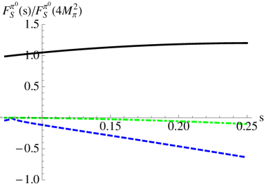
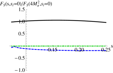
Figure 1: Contributions, as functions of $s$ (in GeV²), to $F_{S}^{\pi^{0}}(s)$ normalised to its value at $s=4M_{\pi}^{2}$: ${\cal F}_{0}^{\pi^{0}}(s)$ (black solid), ${\rm Re}\,{\cal F}_{1}^{\pi^{0}}(s)$ (blue dashed), and ${\rm Im}\,{\cal F}_{1;{\mbox{\scriptsize{data}}}}^{\pi^{0}}(s)$ (green dotted-dashed). The left panel corresponds to our representation (III.7), (III.8), and (III.1) of the exact form factors with the values of the parameters discussed in the text. The right panel corresponds to the parameterisation used by NA48/2 in Ref. Batley:2014xwa for the $K_{e4}^{00}$ form factor, with the parameters chosen as described in the text after Eq. (III.15).

III.2 Phenomenological parameterisations

In order to mimic the situation in $K_{e4}$ decays, the pseudo-data generated with the exact scalar form factors of the pion will now be analyzed using approximate phenomenological parameterisations. For the analysis itself, we will consider a framework close to the experimental set up for the $K_{e4}^{+-}$ Batley:2012rf ; Batley:2007zz ; Batley:2010zza and the $K_{e4}^{00}$ Batley:2014xwa decay channels. From here on, we therefore also use $q^{2}\equiv s/4M_{\pi}^{2}-1$ in addition to $s$, the square of the center-of-mass energy of the dipion system. The region below the cusp corresponds to $q^{2}\leq 0$, while positive values of $q^{2}$ describe the region above the cusp.

For the charged-pion form factor, this means that we consider a parameterisation of the form

$$F_{S}^{\pi}(s)=f_{s}\left[1+\frac{f^{\prime}_{s}}{f_{s}}q^{2}+\frac{f^{\prime\prime}_{s}}{f_{s}}q^{4}+\frac{f^{\prime\prime\prime}_{s}}{f_{s}}q^{6}\right],$$ (III.16)

In the case of the neutral-pion form factor, we consider two parameterisations:

• Model 1:

  $${\cal F}_{0}^{\pi^{0}}(s)=f_{s0}\left[1+\frac{f^{\prime}_{s0}}{f_{s0}}q^{2}+\frac{f^{\prime\prime}_{s0}}{f_{s0}}q^{4}\right]\qquad{\cal F}_{1}^{\pi^{0}}(s)=-2/3(a_{0}^{0}-a_{0}^{2})f_{s}\hat{\sigma}(s)$$ (III.17)

• Model 2:

  $$\!\!{\cal F}_{0}^{\pi^{0}}(s)=f_{s0}\left[1+\frac{f^{\prime}_{s0}}{f_{s0}}q^{2}+\frac{f^{\prime\prime}_{s0}}{f_{s0}}q^{4}\right]\qquad{\cal F}_{1}^{\pi^{0}}(s)=\hat{\sigma}(s)\varphi_{0}^{x}(s)f_{s}\left[1+\frac{f^{\prime}_{s}}{f_{s}}q^{2}+\frac{f^{\prime\prime}_{s}}{f_{s}}q^{4}+\frac{f^{\prime\prime\prime}_{s}}{f_{s}}q^{6}\right]e^{-\frac{i}{2}\sigma_{0}(s)\varphi_{0}^{x}(s)}$$ (III.18)

In order to check the influence of possible higher-order terms in the $q^{2}$ expansion, as compared to the parameterisation considered in Ref. Batley:2014xwa , we have introduced a coefficient $f^{\prime\prime\prime}_{s}$, which can be set to zero or kept as a free variable in the fit.

The first parameterisation with $f^{\prime\prime\prime}_{s}=0$ reproduces exactly the one that was considered in Sec. 9.4 in Ref. Batley:2014xwa . The second parameterisation incorporates more information gathered from the theoretical discussion in Section II, while remaining sufficiently simple. Although we have chosen not to distinguish them, the parameters $f_{s}$, $f^{\prime}_{s}$, $f^{\prime\prime}_{s}$, and $f^{\prime\prime\prime}_{s}$ appearing in Eqs. (III.17) and (III.18) are not, a priori, identical to those occurring in the expression (III.16). One issue of the analysis we will present is precisely to determine to which extent e.g. $f_{s}$ in Eq. (III.17) should be expected to agree with $f_{s}$ in Eq. (III.16). Our first task is therefore to provide reference values for the various parameters. This is done by performing, in Eqs. (III.8) and (III.10) the Taylor expansion around $q^{2}=0$, thus obtaining $f_{s0},f^{\prime}_{s0},f^{\prime\prime}_{s0}$ from the former, and $f_{s},f^{\prime}_{s},f^{\prime\prime}_{s},f^{\prime\prime\prime}_{s}$ from the latter. In the case of $F_{S}^{\pi}(s)$, we neglect the small half-integer powers of $q$ arising in the expansion, which do not contribute significantly in the vicinity of $q^{2}=0$. The resulting values are shown in the last column of Table 1. These expansions are not supposed to provide accurate descriptions of the corresponding form factors over the whole physical range.

The comparison with our various fits will illustrate how different the parameters extracted from the fit and those describing the real Taylor expansion can be, and will thus give information on the possible bias introduced by the fitting procedure. For convenience, in the following $f_{s0},f^{\prime}_{s0}\ldots$ will be called “neutral” parameters, whereas $f_{s},f^{\prime}_{s}\ldots$ are referred to as the “charged” parameters.

III.3 Fitting procedures

In order to stay close to the NA48/2 experimental set up, we will thus assume that we have measurements of $|F^{\pi^{0}}_{S}(s)|^{2}$ at the 12 points corresponding to the barycenters of the experimental bins, and we assign a statistical uncertainty derived from the number of events collected in each bin ($\sim 2900$ events in the first two bins, and $\sim 5900$ events in all the other ones), without any correlations between the bins. As the parameterisations given in Eqs. (III.17) and (III.18) depend on the $S$-wave $\pi\pi$ scattering lengths, our $\chi^{2}$ will also include an uncertainty on these quantities in order to mock up the fact that in the real analysis these scattering lengths are determined from the charged form factor. Here we will use the experimental information on these quantities, namely the latest NA48/2 combination of $K\to 3\pi$ and $K_{\ell 4}$ results Batley:2010zza

$$a_{0}^{0}=0.2210\pm 0.0047\pm 0.0040\,,\quad a_{0}^{2}=-0.0429\pm 0.0044\pm 0.0028\,,\quad\rho_{a_{0}^{0},a_{0}^{2}}=0.92\,,$$ (III.19)

where we combine statistical and systematic uncertainties in quadrature. One should notice that the central values are close (but not identical) to the “true” values used to generate our pseudo-data.

We consider the following methods to determine the coefficients of the above models.

• Method A: fit of $|F^{\pi^{0}}_{S}(s)|^{2}$ for all points to determine all the (neutral, charged) parameters (setting $f^{\prime\prime\prime}_{s}=0$ to ensure a reasonable convergence of the fit), assuming the equality of the neutral and charged normalisation ($f_{s}=f_{s0}$)

• Method B: fit of $|F^{\pi^{0}}_{S}(s)|^{2}$ for all points to determine all the (neutral, charged) parameters, setting $f^{\prime\prime\prime}_{s}=0$ and keeping the normalisations $f_{s}$ and $f_{s0}$ distinct

• Method C: fit of $|F^{\pi^{0}}_{S}(s)|^{2}$ to determine the neutral parameters, injecting information on charged parameters by adding to the $\chi^{2}$ a contribution corresponding to a fit of the charged form factor $F^{\pi}_{S}(s)$ to the polynomial expression (III.16), effectively identifying the charged parameters in the models for $F^{\pi^{0}}_{S}(s)$ with the parameters occurring in the charged scalar form factor.

In method C, we generate pseudo-data points for the charged-pion scalar form factor with energies corresponding to the barycenters given in ref. Batley:2012rf , and use the relative uncertainties for $F_{S}$ (combined in quadrature) quoted for each bin in this reference, without correlations. In agreement with ref. Batley:2012rf , we add an overall 0.62% relative uncertainty, completely correlated between all the charged bins. The curvature of the charged form factor $F^{\pi}_{S}(s)$ being more pronounced than that of the scalar $K_{e4}^{\pm}$ form factor, a $q^{6}$ term must be included in the polynomial in order to obtain a good description of the form factor over the whole kinematic range.

We give the resulting $\chi^{2}_{\min}$ (obtained from the best-fit values of each method). Even though each model provides through its fit a value of $f_{s0}$, one can also determine the latter by considering the branching ratio. In this case, $f_{s0}$ is determined by integrating the decay distribution obtained by using as inputs the slope parameters determined from the different methods of fitting, and fixing the normalisation by comparison with the total decay rate $\Gamma^{\pi^{0}}$ defined in Eq. (III.2), and evaluated with the exact form factor ${F}_{S;{\mbox{\scriptsize{data}}}}^{\pi^{0}}(s)$. The corresponding numerical value is given in Eq. (III.15). We denote by $r$ the ratio between the value of $f_{s0}$ determined this way from the branching ratio, and the true value computed from the exact form factor, i.e. the reference value $f_{s0}=1.381$.

III.4 Discussion of the results

In order to obtain an estimate of the uncertainty attached to the coefficients of models 1-2 using methods A and B, we will perform fits of the models on a series of 10000 pseudo-experiments, generated by assuming that the data are random variables with a mean given by our theoretical model for the neutral scalar form factor and a standard deviation given by the relative uncertainty of the corresponding form factor measured in $K_{e4}$ decays by the NA48 experiment Batley:2012rf ; Batley:2014xwa . We will then determine the mean and the variance of the resulting distribution for each coefficient of the parameterisation considered. The results are gathered in Table. 1. The column labeled “reference” provides a comparison with the coefficients obtained from the Taylor expansions of the form factors given in Eqs. (III.8) and (III.10), as described after Eq. (III.18).

	A1	A2	Reference
$\chi^{2}/N_{dof}$	$(9.1\pm 4.3)/9$	$(6.9\pm 3.6)/7$
$f_{s0}/F_{S}^{\pi}(0)=f_{s}/F_{S}^{\pi}(0)$	$1.38\pm 0.01$	$1.38\pm 0.01$	(1.381,1.395)
$f^{\prime}_{s0}/f_{s0}$	$0.18\pm 0.03$	$0.23\pm 0.03$	0.191
$f^{\prime\prime}_{s0}/f_{s0}$	$\!\!\!\!-0.03\pm 0.03$	$\!\!\!\!-0.33\pm 0.44$	$\!\!\!\!-0.059$
$f^{\prime}_{s}/f_{s}$	0	$1.91\pm 6.31$	0.199
$f^{\prime\prime}_{s}/f_{s}$	0	$\!\!\!\!-1.01\pm 6.38$	$\!\!\!\!-0.032$
$r$	$1.00\pm 0.01$	$0.98\pm 0.04$	1
	B1	B2	Reference
$\chi^{2}/N_{dof}$	$(8.0\pm 4.0)/8$	$(6.0\pm 3.2)/6$
$f_{s0}/F_{S}^{\pi}(0)$	$1.38\pm 0.01$	$1.38\pm 0.01$	1.381
$f^{\prime}_{s0}/f_{s0}$	$0.18\pm 0.04$	$0.21\pm 0.12$	0.191
$f^{\prime\prime}_{s0}/f_{s0}$	$\!\!\!\!-0.03\pm 0.04$	$\!\!\!\!-0.27\pm 0.39$	$\!\!\!\!-0.059$
$f_{s}/f_{s0}$	$1.33\pm 0.40$	$0.97\pm 0.45$	1.010
$f^{\prime}_{s}/f_{s}$	0	$0.43\pm 12.8$	0.199
$f^{\prime\prime}_{s}/f_{s}$	0	$0.95\pm 14.6$	$\!\!\!\!-0.032$
$r$	$1.00\pm 0.01$	$0.97\pm 0.05$	1
	C1	C2	Reference
$\chi^{2}/N_{dof}$	$(3.3\pm 0.1)\cdot 10^{6}/18$	$(15.0\pm 5.6)/16$
$f_{s0}/F_{S}^{\pi}(0)$	$1.38\pm 0.01$	$1.38\pm 0.01$	1.381
$f^{\prime}_{s0}/f_{s0}$	$0.17\pm 0.03$	$0.19\pm 0.03$	0.191
$f^{\prime\prime}_{s0}/f_{s0}$	$\!\!\!\!-0.02\pm 0.03$	$\!\!\!\!-0.04\pm 0.04$	$\!\!\!\!-0.059$
$f_{s}/f_{s0}$	$1.07\pm 0.01$	$1.01\pm 0.01$	1.010
$f^{\prime}_{s}/f_{s}$	0	$0.19\pm 0.01$	0.199
$f^{\prime\prime}_{s}/f_{s}$	0	$\!\!\!\!-0.03\pm 0.01$	$\!\!\!\!-0.032$
$f^{\prime\prime\prime}_{s}/f_{s}$	0	$0.01\pm 0.01$	0.012
$r$	$1.00\pm 0.01$	$1.00\pm 0.02$	1

Table 1: Results of the different models (1-2) and methods (A-B-C), compared to the reference values, obtained from the Taylor expansion of the exact form factors (III.7), (III.8), and (III.1) with the values of the parameters discussed in the text. The value of the ratio $r$ does not result from the fit, but is obtained once the fit has been performed, see the last paragraph of Section III.3. The column label A1 (A2) refers to the fit method A using Model 1 (2), and so on.

As shown by the comparison between Models 1 and 2 for methods A and B, the higher powers of $q^{2}$ are only weakly constrained. Model 1 is very rough and provides a very poor description of the charged form factor (modelling it as a simple constant), which explains the very bad $\chi^{2}_{\rm min}$ for method C1. Only $f_{s0}$ and $f^{\prime}_{s0}/f_{s0}$ can be determined with a good accuracy, but there is no significant bias introduced by the fitting procedure with respect to the reference values. Despite of its shortcomings, method A gives good results for the neutral parameters. As expected, compared to method B, method C provides a much better accuracy on the neutral parameters since the charged ones are constrained in this method. As shown by the ratio $r$, both methods yield accurate values of $f_{s0}$ (at the few percent level) obtained by integrating over the phase space to consider the branching ratio, even methods that do not attempt at describing the $q^{2}<0$ region correctly. This can be easily understood: both methods are constrained to describe correctly $|F_{S}^{\pi^{0}}(s)|^{2}$ for small $q^{2}>0$ (as can be seen by their agreement concerning $f_{s0}$ and $f^{\prime}_{s0}$), but they may differ for $q^{2}<0$ (which exhibit larger uncertainties). However, this region is very narrow ($4M_{\pi^{0}}^{2}\leq s\leq 4M_{\pi}^{2}$) and its contribution is further suppressed by phase space. Therefore, the impact of this region on the estimation of the branching ratio is very small, and the latter is completely dominated by the region $s\geq 4M_{\pi}^{2}$ where all parameterisations agree (the uncertainties reflecting mainly the uncertainties of the inputs and the lack of data at large $q^{2}$).

From this discussion, one thus expects that using the fit function given by Eq. (9.1) of Ref. Batley:2014xwa , and described at the beginning of Sec. II, will lead to similar results for the ratio $r$, despite the fact that this model complies with the expected structure of the cusp only if one imposes strong assumptions, and should be considered as a mere phenomenological parametrisation to reproduce data smoothly. One indeed obtains $r=1\pm 0.01$ and $\chi^{2}/N_{dof}=(8.0\pm 4.1)/9$ for method A, and $r=1\pm 0.01$ and $\chi^{2}/N_{dof}=(8.1\pm 4.1)/8$ for method B, illustrating once more that a smooth parametrisation of the curve above the cusp in good agreement with the data is enough to obtain an accurate and unbiased value for the normalisation $f_{s0}$.

The outcome of this discussion is that the measurement of $|F_{S}^{\pi^{0}}|^{2}$ allows for an accurate determination of $f_{s0}$ (at the percent level), in the current experimental setting. As shown by the ratio $r$, the value of $f_{s0}$ obtained from the computation of the branching ratio is equal (within uncertainties) to its true value for all methods and parameterisations considered here. Even though one has to keep in mind that this observation is done using the pion scalar form factors rather than the actual $K_{\ell 4}$ form factors, it nevertheless suggests that the fit procedure adopted in Ref. Batley:2014xwa does not bias the determination of $f_{s0}$, and thus cannot explain the surprisingly higher value of $f_{s}$ extracted by the NA48/2 collaboration from the $K^{00}_{e4}$ channel, as compared to the value for $f_{s}$ determined from the $K^{+-}_{e4}$ channel.

	D2	D2 with $\sigma[K_{\ell 4}^{00}]/10$	Reference ($s0$, $s$)
$\chi^{2}/N_{dof}$	$(4.8\pm 3.1)/5$	$(5.6\pm 3.3)/7$
$f_{s0}/F_{S}^{\pi}(0)=f_{s}/F_{S}^{\pi}(0)$	$1.38\pm 0.01$	$1.38\pm 0.01$	(1.381,1.395)
$f^{\prime}_{s0}/f_{s0}$	$0.20\pm 0.12$	$0.20\pm 0.01$	0.191
$f^{\prime\prime}_{s0}/f_{s0}$	$0.21\pm 0.88$	$\!\!\!\!-0.05\pm 0.06$	$\!\!\!\!-$0.059
$f^{\prime}_{s}/f_{s}$	$\!-14\pm 234$	$0.62\pm 1.86$	0.199
$f^{\prime\prime}_{s}/f_{s}$	$~{}~{}32\pm 516$	$0.00\pm 3.95$	$\!\!\!\!-$0.032
$a_{0}^{0}-a_{0}^{2}$	$0.21\pm 0.16$	$0.25\pm 0.03$	0.265
$a_{0}^{2}$	$\!\!\!\!-0.83\pm 2.87$	$0.00\pm 0.43$	$\!\!\!\!-$0.045
$r$	$0.92\pm 0.15$	$0.99\pm 0.02$	1
	E2	E2 with $\sigma[K_{\ell 4}^{00}]/10$	Reference
$\chi^{2}/N_{dof}$	$(13.2\pm 5.2)/14$	$(12.9\pm 5.1)/14$
$f_{s0}/F_{S}^{\pi}(0)$	$1.38\pm 0.01$	$1.38\pm 0.01$	1.381
$f^{\prime}_{s0}/f_{s0}$	$0.22\pm 0.05$	$0.20\pm 0.01$	0.191
$f^{\prime\prime}_{s0}/f_{s0}$	$\!\!\!\!-0.09\pm 0.08$	$\!\!\!\!-0.05\pm 0.02$	$\!\!\!\!-$0.059
$f_{s}/f_{s0}$	$1.01\pm 0.01$	$1.01\pm 0.01$	1.010
$f^{\prime}_{s}/f_{s}$	$0.19\pm 0.01$	$0.19\pm 0.01$	0.199
$f^{\prime\prime}_{s}/f_{s}$	$\!\!\!\!-0.03\pm 0.01$	$\!\!\!\!-0.03\pm 0.01$	$\!\!\!\!-$0.032
$f^{\prime\prime\prime}_{s}/f_{s}$	$0.01\pm 0.01$	$0.01\pm 0.01$	0.012
$a_{0}^{0}-a_{0}^{2}$	$0.25\pm 0.10$	$0.26\pm 0.03$	0.265
$a_{0}^{2}$	$0.05\pm 0.16$	$0.07\pm 0.53$	$\!\!\!\!-$0.045
$r$	$1.00\pm 0.01$	$1.00\pm 0.01$	1

Table 2: Results for methods D2 and E2, where $\pi\pi$ scattering lengths are fitted in addition to data on the neutral scalar form factor (for method D) or for both neutral and charged scalar form factors (method E). The third column corresponds to the case where the uncertainties for the neutral scalar form factor are divided by 10.

III.5 Constraining the scattering lengths

The presence of a cusp similar to the one observed in the three-body $K^{+}\to\pi^{+}\pi^{0}\pi^{0}$ decay suggests that it should, in principle, be possible to extract information on the scattering lengths from an accurate measurement of the $K_{e4}^{00}$ differential decay rate. At leading order, the cusp is related to the difference of scattering lengths $a_{0}^{0}-a_{0}^{2}$. Going to higher orders in ${\cal F}_{1}^{\pi^{0}}$ (i.e. including $\varphi_{0}^{x}$) will also add a (weaker) dependence on $a_{0}^{2}$. The scattering lengths can be determined only once the relative normalisation of form factors involved in ${\cal F}_{0}^{\pi^{0}}$ and ${\cal F}_{1}^{\pi^{0}}$ is fixed, which requires the determination of the charged parameters in some way. We define two methods for this purpose. Method D is exactly as method A, without including any experimental information on $a_{0}^{0}$ and $a_{0}^{2}$ in the $\chi^{2}$ [i.e. removing them from the $\chi^{2}$ as described in eq. (III.19)], and similarly for method E with respect to method C. We proceed as before, but now also fitting the scattering lengths.

We consider model 2, as model 1 yielded poor results in the previous section for method C. In order to discuss the potential impact future experimental improvements could have, we consider also a situation where all statistical errors are reduced by 10 (but the number of bins is unchanged) for the neutral channel, keeping the uncertainties unchanged for the charged channel.

The results gathered in Table 2 show that the current statistical uncertainties yield a relative uncertainty on $a_{0}^{0}-a_{0}^{2}$ of around 80% for D2 and 40% for E2. For D2, the charged parameters are only very poorly constrained, but this does not prevent the fit to be reasonable. Reducing the statistical uncertainties by 10 (for the neutral part) yields a significant reduction in the uncertainties, leading to a relative uncertainty on $a_{0}^{0}-a_{0}^{2}$ of 27% for D2 and 10% for E2. At this level of accuracy, there is no significant bias in the value of $a_{0}^{0}-a_{0}^{2}$ extracted through these various approaches. As expected, no relevant information can be obtained on $a_{0}^{2}$, due to the very small sensitivity of the neutral-pion channel to this quantity. To illustrate this point, if instead we fix the value of $a_{0}^{2}$ to its central value in Eq. (III.19), our results concerning the uncertainty on $a_{0}^{0}-a_{0}^{2}$ and the quality of the fit remain unchanged.

From this discussion, one can hope to get some information on $a_{0}^{0}-a_{0}^{2}$ using model 2, should a larger data set become available for $K_{e4}^{00}$ in the future. One has however to keep in mind that we have assumed the equality between the charged and neutral normalisations in the polynomials for the neutral scalar form factors in the case of method D, as well as the equality between the charged parameters in the polynomials for the charged and neutral scalar form factors in the case of method E. These assumptions are certainly reasonable considering the current uncertainties involved, but one might need to reassess them in the presence of more accurate data. In this context, it is also interesting to notice that the current result from the DIRAC experiment Ref. Adeva:2011tc is $|a_{0}^{0}-a_{0}^{2}|=0.253\pm 0.011$, i.e. a 4.3% uncertainty, so that a substantial increase of the statistical sample of $K_{e4}^{00}$ decays is needed in order to reach a comparable accuracy.

IV Radiative corrections to the $K_{e4}^{00}$ decay rate

In this Section we now discuss radiative corrections, which were addressed differently in the analyses of the $K^{+-}_{e4}$ and $K^{00}_{e4}$ channels so far. In the latter case, no radiative corrections were applied to the decay rate measured in Ref. Batley:2014xwa . This accounts for the unspecified factor $\delta_{EM}$ in Eq. (I.1). It is thus natural to ask how much the observed 6.5% discrepancy [see Eq. (I.2)] in the normalisation of the form factor measured in the two channels is due to this correction factor. Our aim here is not to provide a complete discussion of radiative corrections in the $K_{e4}$ decay channels at a level of sophistication that would match the treatment of isospin breaking due to the difference between masses of the charged and neutral pions. We rather want to work out these corrections in a somewhat simpler framework, trying to reproduce a treatment of radiative corrections in the neutral channel similar to the one that was applied in the charged channel, in order to make the comparison as meaningful as possible.

IV.1 Treatment of radiative corrections in $K_{e4}^{+-}$ data

Let us recall how radiative corrections are treated in the charged channel Batley:2007zz ; Batley:2010zza . First, virtual photon exchange between all possible pairs of charged external lines are considered, and the corresponding Sommerfeld-Gamow-Sakharov factors are applied. The corrections induced by emission of real photons are treated with PHOTOS Barberio:1993qi ; Golonka:2005pn ; Nanava:2006vv ; XuWas10 . The latter also implements the wave-function renormalisation on the external charged legs. The couplings of photons to mesons are treated as point-like interactions, given by scalar QED. The result is then free from infrared singularities. Furthermore, one neglects the contributions that vanish when the electron mass goes to zero, which is a sensible limit to consider for the $K_{e4}$ decay channels.

Apart from the Sommerfeld-Gamow-Sakharov factors, some contributions that would arise within a more systematic approach, provided by the effective low-energy theory of QCD and QED for light quarks and leptons Gasser:1984gg ; Urech:1994hd ; Knecht:1999ag , as applied in Refs. Vesna04 ; Cuplov:2003bj ; Stoffer:2013sfa to the channel with two charged pions, are not considered. These include, for instance, all structure-dependent corrections, where the photon is emitted from the tree-level $K_{e4}$ vertices or from internal charged lines. The outcome of such a truncated calculation is affected by an ultraviolet divergence, which is removed by renormalizing the coupling $|V_{us}|^{2}G_{\rm F}^{2}$ [note that in Eq. (12) of Ref. XuWas10 the factor $(\alpha/\pi)$ has been inadvertently omitted],

$$\left(|V_{us}|^{2}G_{\rm F}^{2}\right)^{\rm bare}\left(1-\frac{9}{4}\frac{\alpha}{\pi}\ln\frac{\Lambda^{2}}{M_{\pi}^{2}}\right)=|V_{us}|^{2}G_{\rm F}^{2}.$$ (IV.20)

This same correction factor also appears in Ref. Bystritskiy:2009iv , with the ultraviolet cut-off $\Lambda$ taken equal to $M_{W}$. From this last reference, we also see that the factor $9/4$ decomposes as $9/4=3\times(1/2)-1/4+1/2+1/2$, where the first contribution comes from the wave-function renormalisation of the three charged mesons, the second from the (charged) lepton wave-function renormalisation, and the last two ones from the virtual photon loops between the charged kaon and the charged lepton on the one hand, and between the two charged pions on the other hand [the remaining divergencent contributions of this type, i.e. a photon line connecting the external kaon to the charged-pion lines, or the charged lepton with each of the two pions, cancel pairwise].

In the case of the $K^{00}_{e4}$ channel, we therefore expect that this factor becomes $1\times(1/2)-1/4+1/2=3/4$. Since it differs from the previous one, it cannot be absorbed by the renormalisation of the same prefactor $|V_{us}|^{2}G_{\rm F}^{2}$ as before. It seems more natural instead to absorb these ultraviolet divergences into the normalisations of the form factors

$$f_{s}^{\rm bare}\left(1-\frac{9}{8}\frac{\alpha}{\pi}\ln\frac{\Lambda^{2}}{M_{\pi}^{2}}\right)=f_{s},\qquad f_{s0}^{\rm bare}\left(1-\frac{3}{8}\frac{\alpha}{\pi}\ln\frac{\Lambda^{2}}{M_{\pi}^{2}}\right)=f_{s0}.$$ (IV.21)

This is also more in line with the effective theory approach mentioned above, where the form factors are also corrected by (different) contributions from the low-energy constants $K_{i}$ Urech:1994hd or $X_{i}$ Knecht:1999ag , which are renormalised by the ultraviolet divergences coming from the photon loops. Using instead Eq. (IV.20) in both cases would leave a remaining cut-off dependent contribution to the $K_{e4}^{00}$ amplitude. For a typical value of $\Lambda=1$ GeV, this would modify Eq. (V.55) at the per mille level.

IV.2 Radiative corrections à la PHOTOS for the $K_{e4}^{00}$ decay rate

In the following, we will try to estimate the potential impact of PHOTOS on $K_{e4}^{00}$ rather than pursuing an effective field theory approach. If we want to reproduce the analogue of the PHOTOS treatment XuWas10 of radiative corrections for the $K_{e4}^{00}$ decay rate, we need to consider the wave-function renormalization of the charged lepton and of the kaon in (scalar) QED, and the vertex correction corresponding to diagram $(a)$ in Fig. 2. Using a Pauli-Villars regularization, and taking the photon propagator in the Feynman gauge, we reproduce the expressions of Eq. (6) in Ref. Bystritskiy:2009iv for the former. In order to evaluate and discuss the contribution from diagram $(a)$ in Fig. 2, we chose to describe the tree-level $K_{\ell 4}^{00}$ vertex as

$$A_{\mu}=-i\frac{1}{M_{K}}\left[F^{00}(p_{1}+p_{2})_{\mu}+R^{00}(k-p_{1}-p_{2})_{\mu}\right].$$ (IV.22)

with constant form factors [Bose symmetry forbids a contribution of the form $G^{00}(p_{1}-p_{2})_{\mu}$ with $G^{00}$ constant], so that the lowest-order amplitude reads

$${\cal A}_{0}(K^{00}_{e4})\equiv\frac{i}{M_{K}}\frac{G_{\rm F}}{\sqrt{2}}V_{us}{\bar{\rm u}}(p_{e})\gamma^{\mu}(1-\gamma_{5}){\rm v}(p_{\nu})\left[F^{00}(p_{1}+p_{2})_{\mu}+R^{00}(k-p_{1}-p_{2})_{\mu}\right].$$ (IV.23)

In the limit $m_{e}\to 0$, we obtain

$${\cal A}(K^{00}_{e4};\ref{fig:virtual}(a)) = e^{2}{\cal A}_{0}(K^{00}_{e4})\left[\frac{1}{16\pi^{2}}\left(\ln\frac{\Lambda^{2}}{M_{K}^{2}}+1\right)+4(k\cdot p_{e})C\left((k-p_{e})^{2};M_{K},m_{e}\right)\right.$$

$$\left.\qquad-\,2M_{K}^{2}C_{11}\left((k-p_{e})^{2};M_{K},m_{e}\right)-4(k\cdot p_{e})C_{12}\left((k-p_{e})^{2};M_{K},m_{e}\right)\right]$$

$$\!\!\!\!+\,i\,\frac{e^{2}}{M_{K}}\frac{G_{\rm F}}{\sqrt{2}}V_{us}\,R^{00}(p_{1}+p_{2})_{\nu}\times{\bar{\rm u}}(p_{e})\gamma^{\nu}(1-\gamma_{5}){\rm v}(p_{\nu_{e}})$$

$$\times\left[\frac{1}{32\pi^{2}}\left(3\ln\frac{\Lambda^{2}}{M_{K}^{2}}+\frac{1}{2}\right)-4(k\cdot p_{e})C_{11}\left((k-p_{e})^{2};M_{K},m_{e}\right)+2{\bar{J}}\left((k-p_{e})^{2};M_{K},m_{e}\right)\right].$$

The various loop functions occurring in this expression are defined in Appendix B. Adding to it the wave-function renormalizations on the charged external lines gives the following result, in the framework adopted here, for the radiatively corrected amplitude [$m_{\gamma}$ denotes a small photon mass, introduced as an infrared regulator, to be sent to zero once an infrared-safe observable has been constructed]:

$$\sqrt{Z_{e}}\sqrt{Z_{K}}{\cal A}_{0}(K^{00}_{e4})+{\cal A}(K^{00}_{e4};\ref{fig:virtual}(a)) = {\cal A}_{0}(K^{00}_{e4})\left[1+\frac{e^{2}}{(4\pi)^{2}}\left(\frac{3}{2}\ln\frac{\Lambda^{2}}{M_{\pi}^{2}}-\frac{1}{2}\ln\frac{m_{e}^{2}}{M_{\pi}^{2}}+2\ln\frac{m_{e}^{2}}{m_{\gamma}^{2}}-\ln\frac{M_{K}^{2}}{M_{\pi}^{2}}-2\right)\right.$$ (IV.25)

$$\left.\qquad\ +\,e^{2}\bigg{(}4(k\cdot p_{e})C\left((k-p_{e})^{2};M_{K},m_{e}\right)\right.$$

$$\left.\qquad\quad-\,2M_{K}^{2}C_{11}\left((k-p_{e})^{2};M_{K},m_{e}\right)\right.$$

$$\left.\qquad\quad-4\,(k\cdot p_{e})C_{12}\left((k-p_{e})^{2};M_{K},m_{e}\right)\bigg{)}\right]$$

$$\!\!\!\!+\,i\,\frac{e^{2}}{M_{K}}\frac{G_{\rm F}}{\sqrt{2}}V_{us}\,R^{00}(p_{1}+p_{2})_{\nu}\times{\rm u}(p_{e})\gamma^{\nu}(1-\gamma_{5}){\rm v}(p_{\nu_{e}})$$

$$\!\!\!\times\left[\frac{1}{32\pi^{2}}\left(3\ln\frac{\Lambda^{2}}{M_{K}^{2}}+\frac{1}{2}\right)+2{\bar{J}}\left((k-p_{e})^{2};M_{K},m_{e}\right)\right.$$

$$\left.\qquad\quad-4(k\cdot p_{e})C_{11}\left((k-p_{e})^{2};M_{K},m_{e}\right)\right].$$

We make a few comments about this result:

• Although the result (IV.2) holds in the Feynman gauge $\xi=1$, we have also computed the wave-function renormalisations and ${\cal A}(K^{00}_{e4};\ref{fig:virtual}(a))$ in an arbitrary linear and covariant $\xi$-gauge, and we have checked that the final result (IV.25) does actually not depend on the gauge-fixing parameter $\xi$.

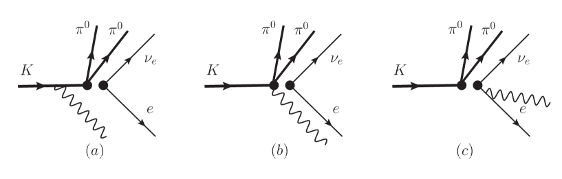
Figure 3: The one-photon emission contributions to the $K^{00}_{e4\gamma}$ decay.

• In order to reproduce the analogue of the PHOTOS treatment Bystritskiy:2009iv ; XuWas10 of radiative corrections for the $K_{e4}^{00}$ decay rate, one needs to add the emission of soft photons from the charged external lines, diagrams $(a)$ and $(c)$ of Fig. 3 [in the $K_{e4}^{+-}$ case, there are two more diagrams where the photon is emitted from the charged pion lines] so that the result is free of infrared singularities at order $\alpha$. These corrections will be discussed later on. At this stage, we simply note that the infrared-divergence of Eq. (IV.25) is equal to

  $$\frac{e^{2}}{(4\pi)^{2}}\,{\cal A}_{0}(K^{00}_{e4})\times\ln m_{\gamma}\left[-4-2(k\cdot p_{e})\tau(k,p_{e})\right],$$ (IV.26)

  with the function $\tau(p_{1},p_{2})$ defined in Eq. (B.96).

• The factor $\frac{3}{8}\frac{\alpha}{\pi}\ln\frac{\Lambda^{2}}{M_{\pi}^{2}}$ discussed in Eq. (IV.21) is indeed to be found in Eq. (IV.25), provided that one sets $R^{00}$ to zero. The only remaining contribution comes from $F^{00}$, which is proportional to $f_{s0}$ at this level. This indeed corresponds to the situation considered in Ref. Bystritskiy:2009iv . In the absence of radiative corrections, the form factor $R^{00}$ [or $R^{+-}$ in the charged channel] does not contribute to the decay distribution for $m_{e}=0$. In this case, one may as well take $R^{00}=0$ from the beginning. But once radiative corrections are switched on, taking $m_{e}=0$ or $R^{00}=0$ are no longer equivalent options. As shown by the second contribution in Eq. (IV.25), there is a correction to $F^{00}$ that is induced by $R^{00}$, and this contribution is not considered in Ref. Bystritskiy:2009iv , and is hence also missing in Ref. XuWas10 .

• At lowest order, and in the isospin limit, one has Bijnens:1989mr

  $$R^{00}=\frac{F^{00}}{2}\left[1+\frac{s_{\pi}}{s_{e}-M_{K}^{2}}\right]=F^{00}\left[\frac{2}{3}-\frac{1}{2}\left(\frac{1}{3}-\frac{s_{\pi}}{s_{e}-M_{K}^{2}}\right)\right].$$ (IV.27)

  Actually, as shown in the second expression, the vertex in the diagram $(a)$ in Fig. 2 only accounts for the contribution $R^{00}=(2/3)\cdot F^{00}$. The second factor comes from the diagram $(f)$ in Fig. 2.

IV.3 Additional non-factorizable radiative corrections to the $K_{e4}^{00}$ decay rate

After these preliminary remarks concerning the PHOTOS-type treatment of radiative corrections in the $K^{+-}_{e4}$ and $K^{00}_{e4}$ channels, let us now address radiative corrections in the channel with two neutral pions in a somewhat more systematic manner. This will allow us to estimate the size of the radiative corrections that are not included in the experimental analysis, as described in the previous section. We keep on considering the limit where $m_{e}$ vanishes, so that in the absence of radiative corrections the amplitude reads simply

$${\cal A}_{0}(K^{00}_{e4})=i\frac{G_{\rm F}}{\sqrt{2}}V_{us}{\bar{\rm u}}(p_{e})\left(\not\!p_{1}+\not\!p_{2}\right)(1-\gamma_{5}){\rm v}(p_{\nu})\times\frac{F^{00}}{M_{K}}+{\cal O}(m_{e}).$$ (IV.28)

For our purpose, it is convenient to distinguish between two types of radiative corrections, that we call factorisable and non-factorisable. Factorisable radiative corrections are defined by the contributions where both ends of the virtual photon line connects to a charged mesonic line or to the vertex with the leptonic current, or when both ends connect to the electron line. These factorisable contributions will not modify the structure of the matrix element, but will change the form factors $F^{00}$ and $R^{00}$. We find it convenient to express them as

$${\cal A}_{\rm fact}(K^{00}_{e4})\equiv i\frac{G_{\rm F}}{\sqrt{2}}V_{us}{\bar{\rm u}}(p_{e})\left(\not\!p_{1}+\not\!p_{2}\right)(1-\gamma_{5}){\rm v}(p_{\nu})\times\frac{F^{00}}{M_{K}}\times\sqrt{Z_{e}}\sqrt{Z_{K}}+{\cal O}(m_{e}),$$ (IV.29)

where we have factored out the wave-function renormalization factors computed in QED for $Z_{e}$, and in scalar QED for $Z_{K}$:

$$\sqrt{Z_{e}} = 1+e^{2}\left[{\bar{\lambda}}-\frac{1}{(4\pi)^{2}}\left(\frac{3}{2}-\frac{1}{2}\ln\frac{m_{e}^{2}}{\mu^{2}}-\ln\frac{m_{e}^{2}}{m_{\gamma}^{2}}\right)\right]$$

$$\sqrt{Z_{K}} = 1+e^{2}\left[-2{\bar{\lambda}}-\frac{1}{(4\pi)^{2}}\left(1+\ln\frac{M_{K}^{2}}{\mu^{2}}-\ln\frac{M_{K}^{2}}{m_{\gamma}^{2}}\right)\right].$$ (IV.30)

In contrast to the preceding subsection, we use now dimensional regularization, with the minimal subtraction of the combination

$${\bar{\lambda}}=\frac{1}{16\pi^{2}}\left[\frac{1}{d-4}-\frac{1}{2}\left(\ln(4\pi)+\Gamma^{\prime}(1)+1\right)\right].$$ (IV.31)

It is understood that $F^{00}$ in Eq. (IV.29) now includes all the remaining factorizable photonic corrections, together with the contributions from the low-energy constants $L_{i}$ Gasser:1984gg and $K_{i}$ Urech:1994hd . These will take care of the UV divergences due to the meson loops and to the photon loops, respectively, so that the product $F^{00}\sqrt{Z_{K}}$ is actually UV finite. It however inherits the infrared divergence contained in $\sqrt{Z_{K}}$.

Let us next consider the non-factorisable contributions. As far as the corrections to ${F}^{00}$ are concerned, they are represented by the diagrams shown in Fig. 2. On finds that the contributions coming from the diagrams $(b)$ and $(c)$ are proportional to the lepton mass, and thus vanish in the limit $m_{e}\to 0$. There are therefore only three diagrams to compute in this approximation. Consistently dropping terms that vanish as $m_{e}\to 0$, one finds that

$${\cal A}(K^{00}_{e4};\ref{fig:virtual}(a)) = {\cal A}_{0}(K^{00}_{e4})\times e^{2}\left[4(k\cdot p_{e})C\left((k-p_{e})^{2};M_{K},m_{e}\right)-2(k\cdot p_{e})C_{12}\left((k-p_{e})^{2};M_{K},m_{e}\right)\right.$$ (IV.32)

$$\left.-{\bar{J}}\left((k-p_{e})^{2};M_{K},m_{e}\right)-4{\bar{\lambda}}-\frac{1}{16\pi^{2}}\left(\ln\frac{M_{K}^{2}}{\mu^{2}}+\ln\frac{m_{e}^{2}}{\mu^{2}}-\frac{10}{3}\right)\right],$$

$${\cal A}(K^{00}_{e4};\ref{fig:virtual}(e))={\cal A}_{0}(K^{00}_{e4})\times\frac{e^{2}}{3}\left[{\bar{J}}\left((k-p_{1}-p_{2})^{2},m_{\gamma},M_{K}\right)-2{\bar{\lambda}}-\frac{1}{16\pi^{2}}\left(\ln\frac{M_{K}^{2}}{\mu^{2}}-1\right)\right],$$ (IV.33)

and

$${\cal A}(K^{00}_{e4};\ref{fig:virtual}(f)) = {\cal A}_{0}(K^{00}_{e4})\times\frac{e^{2}}{2}\left[2(p_{1}+p_{2})^{2}C\left((p_{1}+p_{2})^{2},(k-p_{1}-p_{2})^{2};M_{K},M_{K}\right)\right.$$ (IV.34)

$$\left.-(p_{1}+p_{2})^{2}C_{11}\left((p_{1}+p_{2})^{2},(k-p_{1}-p_{2})^{2};M_{K},M_{K}\right)\right.$$

$$\left.-\frac{2}{3}{\bar{J}}\left((k-p_{1}-p_{2})^{2};m_{\gamma},M_{K}\right)+\frac{7}{3}{\bar{\lambda}}+\frac{1}{16\pi^{2}}\left(\frac{7}{6}\ln\frac{M_{K}^{2}}{\mu^{2}}-\frac{2}{3}\right)\right].$$

Apart from the change of regularization, the expression for ${\cal A}(K^{00}_{e4};\ref{fig:virtual}(a))$ in Eq. (IV.32) reproduces the one of Eq. (IV.2) obtained previously, provided one takes $R^{00}=(2/3)\cdot F^{00}$, as discussed at the end of Sec. IV.2, and makes use of the identities

$$(k\cdot p_{e})C_{11}\left((k-p_{e})^{2};M_{K},m_{e}\right) = -\frac{1}{32\pi^{2}}+\frac{1}{2}{\bar{J}}\left((k-p_{e})^{2};M_{K},m_{e}\right)+\ldots,$$

$$M_{K}^{2}C_{11}\left((k-p_{e})^{2};M_{K},m_{e}\right) = -\frac{1}{32\pi^{2}}\left(1+\ln\frac{M_{K}^{2}}{m_{e}^{2}}\right)+\frac{1}{2}{\bar{J}}\left((k-p_{e})^{2};M_{K},m_{e}\right)$$ (IV.35)

$$-(k\cdot p_{e})C_{12}\left((k-p_{e})^{2};M_{K},m_{e}\right)+\ldots,$$

where the ellipses denote terms that vanish in the limit $m_{e}\to 0$.

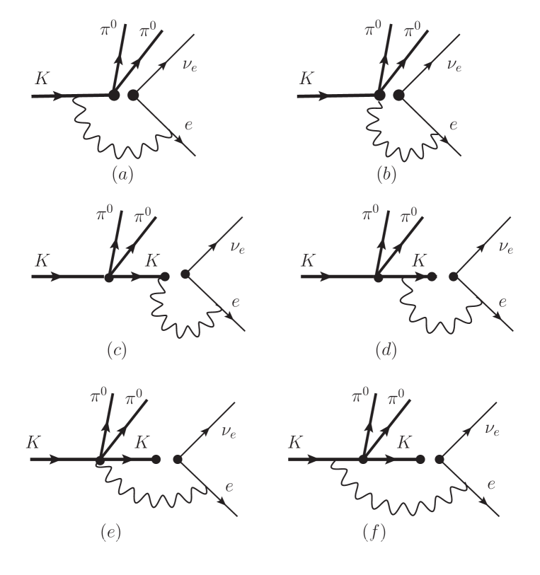
Figure 2: The set of one-loop virtual photon exchange diagrams of the non-factorisable type to consider for the $K^{00}_{e4}$ decay.

Adding up the contributions discussed so far, one obtains an expression for the radiative corrections at order ${\cal O}(\alpha)$ that still contains both infrared and ultraviolet divergences. The latter will be taken care of by the contributions from the counterterms $X_{i}$ introduced in Knecht:1999ag . Their contribution reads

$${\cal A}(K^{00}_{e4};{\rm cts})={\cal A}_{0}(K^{00}_{e4})\times e^{2}\left(-\frac{8}{3}X_{1}-\frac{1}{2}X_{6}\right).$$ (IV.36)

The low-energy constant $X_{1}$ is not renormalized, whereas $X_{6}=X_{6}^{r}(\mu)-5{\bar{\lambda}}$. Collecting the divergent pieces from the various contributions leads to [we recall that at this stage $F^{00}\sqrt{Z_{K}}$ has already been made UV-finite through the contributions of the low-energy constants $L_{i}$ and $K_{i}$]

$${\cal A}(K^{00}_{e4};{\mbox{UV-div}})=e^{2}{\cal A}_{0}(K^{00}_{e4})\times\frac{\bar{\lambda}}{6}\,\bigg{[}\underbrace{-\,24\ }_{\ref{fig:virtual}(a)}\ \underbrace{-\ 4\ }_{\ref{fig:virtual}(e)}\ \underbrace{+\ 7\ }_{\ref{fig:virtual}(f)}\ \underbrace{+\,6\ }_{\sqrt{Z_{e}}}\ \underbrace{+\,15\ }_{X_{6}}\bigg{]}\,=\,0,$$ (IV.37)

which vanishes as it should.

As to the infrared divergences, collecting the IR-divergent pieces contained in the contributions computed so far, one obtains

$${\cal A}(K^{00}_{e4};{\mbox{IR-div}}) = \frac{e^{2}}{(4\pi)^{2}}\,{\cal A}_{0}(K^{00}_{e4})\times\ln m_{\gamma}\bigg{[}\!\underbrace{(-2)}_{\sqrt{Z_{e}}}\,+\,\underbrace{(-2)}_{\sqrt{Z_{K}}}\,+\,\underbrace{(-2)(k\cdot p_{e})\,\tau(k,p_{e})}_{\ref{fig:virtual}(a)}\!\bigg{]},\qquad~{}$$ (IV.38)

with the function $\tau(p_{1},p_{2})$ defined in Eq. (B.96). Besides the wave-function renormalisations, such divergences only arise from the contribution of $C\left((k-p_{\ell})^{2};M_{K},m_{e}\right)$ in ${\cal A}(K^{00}_{e4};1(a))$. Notice that this infrared divergence coincides with the one of the result (IV.25), given in Eq. (IV.26). The construction of an infrared-safe observable at order ${\cal O}(\alpha)$ requires also to consider the process with the emission of one soft photon. The corresponding differential decay rate is given by

$$d\Gamma({K^{00}_{e4\gamma}}) = \frac{1}{2M_{K}}\,\frac{1}{2}\sum_{\rm spins,\,pol.}\left|{\cal A}(K^{00}_{e4\gamma})\right|^{2}\times(2\pi)^{4}\delta^{4}(k-p_{1}-p_{2}-p_{\ell}-p_{\nu}-q)$$ (IV.39)

$$\times\frac{d^{3}{\vec{p}}_{1}}{(2\pi)^{3}2E_{1}}\,\frac{d^{3}{\vec{p}}_{2}}{(2\pi)^{3}2E_{2}}\,\frac{d^{3}{\vec{p}}_{\ell}}{(2\pi)^{3}2E_{\ell}}\,\frac{d^{3}{\vec{p}}_{\nu}}{(2\pi)^{3}2|{\vec{p}}_{\nu}|}\,\frac{d^{3}{\vec{q}}}{(2\pi)^{3}2|{\vec{q}}|}.$$

The amplitude ${\cal A}(K^{00}_{e4\gamma})$ for the radiative decay $K^{\pm}\to\pi^{0}\pi^{0}e^{\pm}\stackrel{{{}_{(-)}}}{{\nu_{e}}}\gamma$ can be expanded in powers of the photon energy,

$${\cal A}(K^{00}_{e4\gamma})={\cal A}_{-1}(K^{00}_{e4\gamma})+{\cal A}_{0}(K^{00}_{e4\gamma})+\ldots$$ (IV.40)

The Low approximation consists in keeping ${\cal A}_{-1}(K^{00}_{e4\gamma})$ alone. This is enough in order to study the emission of only soft photons and to discuss the issue of infrared divergences. Explicitly, one has [$q_{\mu}$ is the momentum of the emitted (real) photon, $\varepsilon^{*}(q)$ the corresponding polarization vector]

$${\cal A}_{-1}(K^{00}_{e4\gamma})=e{\cal A}_{0}(K^{00}_{e4})\left(\frac{p_{\ell}\cdot\varepsilon^{*}(q)}{p_{\ell}\cdot q+\frac{m_{\gamma}^{2}}{2}}\,-\,\frac{k\cdot\varepsilon^{*}(q)}{k\cdot q-\frac{m_{\gamma}^{2}}{2}}\right).$$ (IV.41)

Then

$$\sum_{\rm spins,\,pol.}\left|{\cal A}_{-1}(K^{00}_{e4\gamma})\right|^{2} = -e^{2}\!\sum_{\rm spins}\left|{\cal A}(K^{00}_{e4})\right|^{2}\times\left[\frac{m_{\ell}^{2}}{\left(p_{\ell}\cdot q+\frac{m_{\gamma}^{2}}{2}\right)^{2}}+\frac{M_{K}^{2}}{\left(k\cdot q-\frac{m_{\gamma}^{2}}{2}\right)^{2}}\qquad{}\right.$$ (IV.42)

$$\left.\qquad-2\,\frac{k\cdot p_{\ell}}{\left(p_{\ell}\cdot q+\frac{m_{\gamma}^{2}}{2}\right)\left(k\cdot q-\frac{m_{\gamma}^{2}}{2}\right)}\right].$$

One may then perform the integration over the undetected soft photon. In the soft-photon approximation, the photon momentum in the delta-function of the phase-space integration is neglected, and one takes

$$d\Gamma^{\rm soft}({K^{00}_{e4\gamma}}) = (2\pi)^{4}\delta^{4}(k-p_{1}-p_{2}-p_{\ell}-p_{\nu})\times\frac{d^{3}{\vec{p}}_{1}}{(2\pi)^{3}2E_{1}}\,\frac{d^{3}{\vec{p}}_{2}}{(2\pi)^{3}2E_{2}}\,\frac{d^{3}{\vec{p}}_{\ell}}{(2\pi)^{3}2E_{\ell}}\,\frac{d^{3}{\vec{p}}_{\nu}}{(2\pi)^{3}2|{\vec{p}}_{\nu}|}$$ (IV.43)

$$\times\frac{1}{2M_{K}}\,\frac{1}{2}\int_{|{\vec{q}}|\leq\Delta E}\frac{d^{3}{\vec{q}}}{(2\pi)^{3}2|{\vec{q}}|}\sum_{\rm spins,\,pol.}\left|{\cal A}_{-1}(K^{00}_{e4\gamma})\right|^{2}$$

$$= d\Gamma_{0}({K^{00}_{e4}})\times(-e^{2})\int_{|{\vec{q}}|\leq\Delta E}\frac{d^{3}{\vec{q}}}{(2\pi)^{3}2|{\vec{q}}|}\left[\frac{m_{\ell}^{2}}{\left(p_{\ell}\cdot q+\frac{m_{\gamma}^{2}}{2}\right)^{2}}+\frac{M_{K}^{2}}{\left(k\cdot q-\frac{m_{\gamma}^{2}}{2}\right)^{2}}\qquad{}\right.$$

$$\left.\qquad-2\,\frac{k\cdot p_{\ell}}{\left(p_{\ell}\cdot q+\frac{m_{\gamma}^{2}}{2}\right)\left(k\cdot q-\frac{m_{\gamma}^{2}}{2}\right)}\right].$$

Expressions for the corresponding integrals can be found in Vesna04 ; Stoffer:2013sfa . The integral is limited to photon energies $|{\vec{q}}|$ below the experimental detection threshold $\Delta E$ in the kaon rest-frame. As far as the infrared divergences are concerned, one has

$$d\Gamma^{\rm soft}_{\mbox{\tiny{IR-div}}}({K^{00}_{e4\gamma}})=d\Gamma_{0}({K^{00}_{e4}})\times\frac{e^{2}}{8\pi^{2}}\times\ln m_{\gamma}\left[2+2+2(k\cdot p_{e})\tau(k,p_{e})\right].$$ (IV.44)

Therefore, the contributions proportional to $\ln m_{\gamma}$ cancel in the sum $d\Gamma({K^{00}_{e4}})+d\Gamma({K^{00}_{e4\gamma}})$. For later convenience, we rewrite Eq. (IV.43) in a way that explicitly displays the IR-singular part:

$$d\Gamma^{\rm soft}({K^{00}_{e4\gamma}}) = d\Gamma_{0}({K^{00}_{e4}})\times\frac{e^{2}}{8\pi^{2}}\left[2+(k\cdot p_{e})\tau(k,p_{e})\right]\times 2\ln\frac{m_{\gamma}}{2\Delta E}+d{\bar{\Gamma}}^{\rm soft}({K^{00}_{e4\gamma}}).$$ (IV.45)

We then add the contribution

$${\cal A}_{0}(K^{00}_{e4})\times\frac{e^{2}}{8\pi^{2}}\left[2+(k\cdot p_{e})\tau(k,p_{e})\right]\times 2\ln\frac{m_{\gamma}}{2\Delta E}$$ (IV.46)

to the amplitudes involving virtual photons, such as to make them infrared finite. To this end, we define the function

$${\bar{C}}\left((k-p_{e})^{2};M_{K},m_{e};\Delta E\right)=C\left((k-p_{e})^{2};M_{K},m_{e}\right)+\frac{1}{32\pi^{2}}\,\tau(k,p_{e})\times\ln\frac{m_{\gamma}}{2\Delta E}.$$ (IV.47)

IV.4 Discussion on radiative corrections for $K_{e4}^{00}$

We can now add the virtual and real contributions described up to now which should be involved in a PHOTOS-like treatment of this decay. We include them as a correction of the form $(1+\delta_{\rm EM})$ to the determination of the form factor from the measurement of the branching ratio. To this end, we compute the total decay rate including the soft photon emission

$$\Gamma^{\rm tot}=\Gamma(K_{e4}^{00})+{\bar{\Gamma}}^{\rm soft}({K^{00}_{e4\gamma}}),$$ (IV.48)

where $\Gamma(K_{e4}^{00})$ includes corrections at first order in the fine-structure constant $\alpha$, and write it in terms of the decay rate $\Gamma_{0}(K_{e4}^{00})$ without radiative corrections in the form

$$\Gamma^{\rm tot}=\Gamma_{0}(K_{e4}^{00})\times\left(1+2\delta_{EM}\right).$$ (IV.49)

Let us first discuss the corrections computed in Subsection B above. In order to obtain a result that is as close as possible to the treatment of radiative corrections in the $K_{e4}^{+-}$ channel, we absorb the UV-divergent factor of Eq. (IV.25) in $F^{00}$ and take $R^{00}$ equal to zero. Then $\Gamma(K_{e4}^{00})$ is computed by performing the phase-space integration of

$${\cal A}_{0}(K^{00}_{e4})\left[{\cal A}_{0}(K^{00}_{e4})+2e^{2}\Delta{\cal A}(K^{00}_{e4})\right],$$ (IV.50)

where

$$\Delta{\cal A}(K^{00}_{e4}) = {\cal A}_{0}(K^{00}_{e4})\left[\frac{1}{(4\pi)^{2}}\left(-\frac{1}{2}\ln\frac{m_{e}^{2}}{M_{\pi}^{2}}+4\ln\frac{m_{e}}{2\Delta E}-\ln\frac{M_{K}^{2}}{M_{\pi}^{2}}-2\right)+4(k\cdot p_{e}){\bar{C}}\left((k-p_{e})^{2};M_{K},m_{e};\Delta E\right)\right.$$ (IV.51)

$$\left.\qquad\quad-\,2M_{K}^{2}C_{11}\left((k-p_{e})^{2};M_{K},m_{e}\right)-4(k\cdot p_{e})C_{12}\left((k-p_{e})^{2};M_{K},m_{e}\right)\right].$$

We take $\Delta E=11.7$ MeV, the value corresponding to the NA48/2 experiment Batley:2014xwa , for the real-photon detection threshold in the kaon rest frame. This gives then

$$\delta_{EM}=0.018.$$ (IV.52)

This value has the expected size. Moreover, it goes into the right direction, in the sense that it reduces the discrepancy in Eq. (I.2) from $6.5\%$ to $4.6\%$.

As a test of the stability of the result (IV.52) we may also evaluate the non-factorizable radiative corrections corresponding to all the diagrams in Fig. 2. This amounts to taking the expressions in Eqs. (IV.32), (IV.33), and (IV.34) for the evaluation of $\Gamma(K_{e4}^{00})$ (let us stress again that these equations have been obtained in a regularisation scheme differing from the one discussed in Sec. IV.2). We absorb the ultraviolet divergences, as well as the contribution (IV.36) into $F^{00}$, in order to build a quantity both UV and IR finite. Constant terms have been discarded as they could be included in the contribution of the counterterms $X_{1}$ and $X_{6}$. The resulting expression for $\Delta{\cal A}(K^{00}_{e4})$ then reads

$$\Delta{\cal A}(K^{00}_{e4}) = {\cal A}_{0}(K^{00}_{e4})\left[\frac{1}{(4\pi)^{2}}\left(-\frac{7}{4}\ln\frac{M_{K}^{2}}{M_{\pi}^{2}}-\frac{1}{2}\ln\frac{m_{e}^{2}}{M_{\pi}^{2}}+2\ln\frac{m_{e}}{2\Delta E}+2\ln\frac{M_{K}}{2\Delta E}\right)\right.$$ (IV.53)

$$\left.\qquad\quad+4(k\cdot p_{e}){\bar{C}}\left((k-p_{e})^{2};M_{K},m_{e};\Delta E\right)\right.$$

$$\left.\qquad\quad-2(k\cdot p_{e})C_{12}\left((k-p_{e})^{2};M_{K},m_{e}\right)-\frac{2}{3}{\bar{J}}\left((k-p_{e})^{2};M_{K},m_{e}\right)\right.$$

$$\left.\qquad\quad+(p_{1}+p_{2})^{2}C\left((p_{1}+p_{2})^{2},(k-p_{1}-p_{2})^{2};M_{K},M_{K}\right)\right.$$

$$\left.\qquad\quad-\frac{1}{2}(p_{1}+p_{2})^{2}C_{11}\left((p_{1}+p_{2})^{2},(k-p_{1}-p_{2})^{2};M_{K},M_{K}\right)\right.$$

$$\left.\qquad\quad-\frac{1}{3}{\bar{J}}\left((k-p_{1}-p_{2})^{2};m_{\gamma},M_{K}\right)\right],$$

instead of the expression in Eq. (IV.51). For $\Delta E=11.7$ MeV, we obtain now

$$\delta_{EM}=0.017.$$ (IV.54)

This value is quite close to the one obtained in Eq. (IV.52), so that in the present case the treatment of radiative corrections à la PHOTOS seems to yield stable results even after the inclusion of non-factorizable contributions.

V Summary and conclusion

The present study is devoted to isospin-breaking effects in the semileptonic decay of the charged kaon into two neutral pions, $K^{\pm}\to\pi^{0}\pi^{0}e^{\pm}\stackrel{{{}_{(-)}}}{{\nu_{e}}}$. Because of the smallness of the electron mass and of the limited experimental precision, this decay can be described in terms of a single form factor. This form factor also occurs in the description of the decay into two charged pions, $K^{\pm}\to\pi^{+}\pi^{-}e^{\pm}\stackrel{{{}_{(-)}}}{{\nu_{e}}}$, and up to isospin-breaking contributions, the two determinations should agree. The present study focuses mainly on two aspects related to this issue: i) to ascertain quantitatively to which extend the phenomenological parameterizations used in order to analyse the data could impinge on the resulting value of the normalization or on the shape of the form factor measured in the decay $K^{\pm}\to\pi^{0}\pi^{0}e^{\pm}\stackrel{{{}_{(-)}}}{{\nu_{e}}}$, and ii) to obtain a quantitative estimate of the radiative corrections to the total decay rate, which again might affect the normalization of the form factor.

Concerning the first issue, we have considered the form factors of the pion as a case study. As a first step, we have discussed the structure of the form factors, and their properties linked to the presence of a cusp, using exact expressions of the form factors valid up to two loops in the low-energy expansion. We have clearly established that the phenomenological parameterizations used in order to analyse the data did not agree with the general properties that can be infered form these exact expressions. In a second step, we have generated pseudo-data from these form factors, that we have then analysed using several phenomenological parameterizations. The outcome of this study is that the determination of the normalization of the form factor is actually not sensitive to the parameterizations used. As a side product, we see that the higher orders in the Taylor expansion of form factors are not accurately determined by a direct fit to simplified (polynomial) formulae. Although our study was carried out for the scalar form factor of the neutral pion, we expect that the conclusion also holds for the $K_{e4}^{00}$ form factor. We have also considered the possibility to constrain the $\pi\pi$ $S$-wave scattering lengths from the measurement of the decay distribution. We have found that, unfortunately, with the sample of events presently available, the statistical uncertainties remain large. A statistical sample comparable to the one available in the $K_{e4}^{+-}$ channel would be required in order to reach a precision close to that obtained by the Dirac experiment.

The second issue addressed in this paper consists in radiative corrections. We have determined the correction factor $\delta_{EM}$ to the total decay rate in Eq. (I.2). In order to make a meaningful comparison with the value of the normalization of the form factor extracted from the $K_{e4}^{+-}$ channel, we have used a simplified framework, including only those corrections that were also included in the latter case (one-loop photonic corrections on the wave functions and tree-level vertex). Our result $\delta_{EM}=0.018$ leads to the replacement of Eq. (I.2) by

$$\frac{f_{s}[K^{00}_{e4}]}{f_{s}[K^{+-}_{e4}]}=1.046(10).$$ (V.55)

Note that the error bar in this equation is purely from experimental origin, and does not include the systematic uncertainties from the methods used for the evaluation of radiative corrections in both channels. Such additional uncertainties can stem, for instance, from the regularisation dependence of the PHOTOS(-like) treatment of radiative corrections, and from neglecting the dependence in the cut off $\Lambda$ discussed in Sec. IV.1.

We have also considered additional photonic corrections estimated within a different regularisation scheme, and we have found that they do not modify the previous estimate in a significant way. A few comments are in order:

• The analysis of radiative corrections we have performed provides an adequate estimate of the global factor $\delta_{EM}$ that modifies the total decay rate. It need not be suitable for an analysis of radiative corrections to the phase-space distribution itself.

• Other isospin-breaking corrections, among them factorizable exchanges of virtual photons, but also effects due to $m_{u}-m_{d}$ or to the mass differences between charged and neutral pions and/or kaons, are not covered by our analysis. They could affect the normalization of the form factors measured in the two channels in different ways. A mode elaborate study is needed in order to reach a quantitatively meaningful interpretation of the result in Eq. (V.55).

• At lowest order in the chiral expansion, these additional isospin-breaking corrections are given by Eq. (I.3). For $R=35.8(1.9)(1.8)$ Aoki:2013ldr , and adding errors in quadrature, we obtain

  $$\left.\frac{f_{s}[K^{00}_{e4}]}{f_{s}[K^{+-}_{e4}]}\right|_{\rm LO}=1.042(3).$$ (V.56)

  In view of the value given in Eq. (V.55), the corrections from higher orders to this ratio should therefore be small.

• Conversely, using the relation (I.3) in regard to the result (V.55), and discarding yet to be computed corrections to the former, we obtain $R=32^{+9}_{-6}$.

The discussion of the radiative corrections presented here is clearly only a first step. In view of the statistical accuracy of the data, a full model-independent calculation of these corrections in the neutral as well as in the charged channels is certainly mandatory before a definite conclusion can be reached concerning the observed difference in the normalisation of the form factors between the neutral and the charged channels. This task is clearly beyond the scope of the present note, and is left for future work.

Appendix A Properties of the functions ${\bar{K}}_{n}^{\alpha}(s)$

In this Appendix, we wish to summarise the properties of the functions ${\bar{K}}_{n}^{\alpha}(s)$ that are needed in the discussion of the cusp in Section II. Let us start with the functions ${\bar{K}}_{n}^{0}(s)$ and ${\bar{K}}_{n}^{{\mbox{\tiny$\nabla$}}}(s)$, defined by dispersive integral as in Eq. (II.41), with $s_{\rm thr}=4M_{\pi^{0}}^{2}$ and KMSF95

$$k_{0}^{0}(s)\,=\,\frac{1}{16\pi}\,\sigma_{0}(s),\qquad k_{1}^{0}(s)\,=\,\frac{1}{8\pi}\,L_{0}(s)\,,$$

$$k_{2}^{0}(s)\,=\,\frac{1}{8\pi}\,\left(1\,-\,\frac{4M_{\pi^{0}}^{2}}{s}\right)\,L_{0}(s)\,,\qquad k_{3}^{0}(s)\,=\,\frac{3}{16\pi}\,\frac{M_{\pi^{0}}^{2}}{s\sigma_{0}(s)}\,L_{0}^{2}(s)\,,$$

$$k_{1}^{{\mbox{\tiny$\nabla$}}}(s)\,=\,\frac{1}{8\pi}\,\frac{\sigma_{0}(s)}{\sigma(s+4\Delta_{\pi})}\,L(s+4\Delta_{\pi})\,,\qquad k_{3}^{{\mbox{\tiny$\nabla$}}}(s)\,=\,\frac{3}{16\pi}\,\frac{M_{\pi}^{2}}{s\sigma_{0}(s)}\,L^{2}(s+4\Delta_{\pi})\,,\qquad.$$ (A.57)

The definitions of the functions $\sigma_{0}(s)$ and $L_{0}(s)$ for $s\geq 4M_{\pi^{0}}^{2}$ can be found in Eqs. (II.17) and (II.20), respectively. The function $\sigma(s)$ is also to be found in Eq. (II.17), whereas $L(s)$ is defined as

$$L(s) = \left\{\begin{array}[]{l}\ln\left(\frac{1-\sigma(s)}{1+\sigma(s)}\right)\equiv{\hat{L}}(s)\ \quad\ \,[s\geq 4M_{\pi}^{2}]\\ \\ \ln\left(\frac{\sigma(s)-1}{\sigma(s)+1}\right)\equiv{\hat{L}}+i\pi\quad[4M_{\pi^{0}}^{2}\leq s\leq 4M_{\pi}^{2}]\\ \end{array}\right.,$$ (A.61)

according to the definitions (II.26) and (II.30). For $s\geq 4M_{\pi^{0}}^{2}$, the functions $k_{n}^{0}(s)$ and $k_{n}^{{\mbox{\tiny$\nabla$}}}(s)$ are real and smooth. In the same range of $s$, the functions ${\bar{K}}_{n}^{0}(s)$ and ${\bar{K}}_{n}^{{\mbox{\tiny$\nabla$}}}(s)$ have smooth real and imaginary parts, with ${\rm Im}\,{\bar{K}}_{n}^{0}(s)=k_{n}^{0}(s)$, ${\rm Im}\,{\bar{K}}_{n}^{{\mbox{\tiny$\nabla$}}}(s)=k_{n}^{{\mbox{\tiny$\nabla$}}}(s)$. Finally, the functions ${\bar{K}}_{n}^{0}(s)$ for $n\geq 1$ can be expressed in terms of ${\bar{J}}_{0}(s)\equiv{\bar{K}}_{0}^{0}(s)$. The explicit expressions and their derivation were given in KMSF95 .

There is not much to add as far as the functions ${\bar{K}}_{n}(s)$ are concerned: it is sufficient to replace everywhere in Eq. (A.57) $M_{\pi^{0}}$ by the charged pion mass $M_{\pi}$, and hence $\sigma_{0}(s)$ by $\sigma(s)$, and $L_{0}(s)$ by $L(s)$. In the dispersive representation (II.41), the integration starts at $s_{\rm thr}=4M_{\pi}^{2}$. In the case of ${\bar{K}}_{0}(s)\equiv{\bar{J}}(s)$, the decomposition (II.24) then follows from (II.53) by noticing that $k_{0}(s)/\sigma(s)$ is a constant, and that KMSF95 ; DescotesGenon:2012gv

$${\rm Re}\,{\bar{J}}(s)=\frac{1}{16\pi^{2}}\left[2+\sigma(s)L(s)\right]\quad\ [s\geq 0].$$ (A.62)

For the remaining functions ${\bar{K}}_{n}(s)$, it is most convenient to use their expressions in terms of ${\bar{J}}(s)$. One then finds

$$16\pi^{2}\bar{K}_{1}^{[0]}=\hat{L}(s)^{2}-\pi^{2} 16\pi^{2}\bar{K}_{1}^{[1]}=-2\pi\frac{\hat{L}(s)}{\sigma(s)}$$

$$16\pi^{2}\bar{K}_{2}^{[0]}=\sigma^{2}(\hat{L}^{2}(s)-\pi^{2})-4 16\pi^{2}\bar{K}_{2}^{[1]}=-2\pi\hat{L}(s)\sigma(s)$$

$$16\pi^{2}\bar{K}_{3}^{[0]}=\hat{L}(s)(\hat{L}^{2}(s)-2\pi^{2})\frac{M_{\pi}^{2}}{s\sigma(s)}-\frac{\pi^{2}}{2} 16\pi^{2}\bar{K}_{3}^{[1]}=-3\pi\frac{M_{\pi}^{2}}{s}\frac{\hat{L}^{2}(s)}{\sigma^{2}(s)}.$$ (A.63)

One may check that all these functions are real and smooth for $s\geq 4M_{\pi^{0}}^{2}$ [actually, for $s\geq 0$].

The functions ${\bar{K}}_{n}^{x}(s)$, $n=1,3$, are defined by

$${\bar{K}}_{n}^{x}(s)=\frac{s}{\pi}\int_{4M_{\pi}^{2}}^{\infty}\frac{dx}{x}\frac{k_{n}^{x}(x)}{x-s-i0},$$ (A.64)

with [the quantities appearing in these formulae are defined in Ref. DescotesGenon:2012gv , see Eqs. (2.13), (4.13), (4.16), and (4.17) therein]

$$k_{1}^{x}(s) = \frac{1}{8\pi}\,\frac{1}{s\sigma_{0}(s)}\left[\lambda^{1/2}(t_{\mbox{\tiny$-$}}(s)){\cal L}_{\mbox{\tiny$-$}}(s)-\lambda^{1/2}(t_{\mbox{\tiny$+$}}(s)){\cal L}_{\mbox{\tiny$+$}}(s)\right],$$

$$k_{2}^{x}(s) = \frac{1}{8\pi}\sigma(s)\sigma_{0}(s)L_{0}(s),$$

$$k_{3}^{x}(s) = \frac{3}{16\pi}\,\frac{M_{\pi}^{2}}{s\sigma_{0}(s)}\left[{\cal L}_{\mbox{\tiny$-$}}^{2}(s)-{\cal L}_{\mbox{\tiny$+$}}^{2}(s)\right].$$ (A.65)

The three functions ${k}_{n}^{x}(s)$, $n=1,2,3$, are real and smooth for $s\geq M_{\pi}^{2}$, and they become purely imaginary for $4M_{\pi^{0}}^{2}\leq s\leq 4M_{\pi}^{2}$. The functions ${\hat{k}}_{n}^{x}(s)\equiv{k}_{n}^{x}(s)/\sigma(s)$ are then smooth in the range $4M_{\pi^{0}}^{2}\leq s\leq M_{K}^{2}$, so that one obtains

$${\bar{K}}_{n}^{x[1]}(s)=-\frac{k_{n}^{x}(s)}{\sigma(s)},$$ (A.66)

and

$${\bar{K}}_{1,3}^{x[0]}(s)\ =\ \left\{\begin{array}[]{l}{\rm Re}\,{\bar{K}}_{1,3}^{x}(s)\qquad\qquad\qquad\quad[s\geq 4M_{\pi}^{2}]\\ \\ {\rm Re}\,{\bar{K}}_{1,3}^{x}(s)+{\displaystyle\frac{{\hat{\sigma}}(s)}{\sigma(s)}}k_{1,3}^{x}(s)\quad[4M_{\pi^{0}}^{2}\leq s\leq 4M_{\pi}^{2}]\end{array}\right..$$ (A.70)

Since analytical expressions for ${\rm Re}\,{\bar{K}}_{1,3}^{x}(s)$ are not available, one has to use the integral representation given in Eq. (A.64) for numerical applications.

Finally, there remains to discuss the function ${\cal K}^{x}(s)$ whose discontinuity along the real $s$ axis for $s\geq 4M_{\pi}^{2}$ reads

$$k^{x}(s)=\frac{1}{16\pi}\frac{M_{\pi}^{2}}{\Delta_{\pi}}\frac{\sigma(s)}{\sigma_{0}(s)}\frac{1}{s}\left[\left(\sigma(s)-\sigma_{0}(s)\right)\lambda^{1/2}(t_{\mbox{\tiny$-$}}(s)){\cal L}_{\mbox{\tiny$-$}}(s)-\,\left(\sigma(s)+\sigma_{0}(s)\right)\lambda^{1/2}(t_{\mbox{\tiny$+$}}(s)){\cal L}_{\mbox{\tiny$+$}}(s)\right].$$ (A.71)

The function $k^{x}(s)/\sigma(s)$ is real and smooth for $s\geq 4M_{\pi^{0}}^{2}$. Thus one infers

$${\bar{\cal K}}^{x[1]}(s)=-\frac{k^{x}(s)}{\sigma(s)},$$ (A.72)

and

$${\bar{\cal K}}^{x[0]}(s)\ =\ \left\{\begin{array}[]{l}{\rm Re}\,{\bar{\cal K}}^{x}(s)\qquad\qquad\qquad\ \ \,[s\geq 4M_{\pi}^{2}]\\ \\ {\rm Re}\,{\bar{\cal K}}^{x}(s)+{\displaystyle\frac{{\hat{\sigma}}(s)}{\sigma(s)}}k^{x}(s)\quad\ [4M_{\pi^{0}}^{2}\leq s\leq 4M_{\pi}^{2}]\end{array}\right..$$ (A.76)

Appendix B Loop functions

The computation, in Section IV of the diagrams describing the virtual photon corrections involves a certain number of loop functions, that are briefly discussed here, in order to make the calculation in section IV self-contained.

At the level of the two-point one-loop diagrams, one has

$$J\left(p^{2};m_{1},m_{2}\right)=\frac{1}{i}\int\frac{d^{4}\ell}{(2\pi)^{4}}\,\frac{1}{(\ell^{2}-m_{1}^{2})[(\ell-p)^{2}-m_{2}^{2}]},$$ (B.77)

and

$$J_{\mu}\left(p~{};m_{1},m_{2}\right) = \frac{1}{i}\int\frac{d^{4}\ell}{(2\pi)^{4}}\,\frac{\ell_{\mu}}{(\ell^{2}-m_{1}^{2})[(\ell-p)^{2}-m_{2}^{2}]}$$ (B.78)

$$= \frac{p_{\mu}}{2p^{2}}\left[\left(p^{2}+m_{1}^{2}-m_{2}^{2}\right)J\left(p^{2};m_{1},m_{2}\right)+iA(m_{1}^{2})-iA(m_{2}^{2})\right],$$

where $A(m^{2})$ is related to the tadpole graph,

$$A(m^{2})=\int\frac{d^{4}\ell}{(2\pi)^{4}}\,\frac{1}{\ell^{2}-m^{2}}=-im^{2}\left[2{\bar{\lambda}}+\frac{1}{16\pi^{2}}\ln\frac{m^{2}}{\mu^{2}}+{\cal O}(d-4)\right].$$ (B.79)

Other useful relations are

$$J(p^{2};m_{1},m_{2})={\bar{J}}(p^{2};m_{1},m_{2})-2{\bar{\lambda}}-\frac{1}{16\pi^{2}}\frac{m_{1}^{2}\ln\frac{m_{1}^{2}}{\mu^{2}}-m_{2}^{2}\ln\frac{m_{2}^{2}}{\mu^{2}}}{m_{1}^{2}-m_{2}^{2}},$$ (B.80)

and

$$J(m^{2};0,m)=-2{\bar{\lambda}}+\frac{1}{16\pi^{2}}\left[1-\ln\frac{m^{2}}{\mu^{2}}\right].$$ (B.81)

Explicit expressions of the function ${\bar{J}}(p^{2};m_{1},m_{2})$ can be found in Ref. Gasser:1984gg . Moreover, the link with the functions ${\bar{J}}(s)$ and ${\bar{J}}_{0}(s)$ encountered in Section II is given by ${\bar{J}}(s)\equiv{\bar{J}}(s;M_{\pi},M_{\pi})$ and ${\bar{J}}_{0}(s)\equiv{\bar{J}}(s;M_{\pi^{0}},M_{\pi^{0}})$.

As far as the three-point one-loop functions are concerned, one has

$$C\left((p_{1}-p_{2})^{2},p^{2}_{2};m_{1},m_{2}\right)=\frac{1}{i}\int\frac{d^{4}\ell}{(2\pi)^{4}}\,\frac{1}{(\ell^{2}-2\ell\cdot p_{1})[(\ell-p_{2})^{2}-m_{2}^{2}](\ell^{2}-m_{\gamma}^{2})},$$ (B.82)

and

$$C_{\mu}\left(p_{1},p_{2};m_{1},m_{2}\right) = \frac{1}{i}\int\frac{d^{4}\ell}{(2\pi)^{4}}\,\frac{\ell_{\mu}}{(\ell^{2}-2\ell\cdot p_{1})[(\ell-p_{2})^{2}-m_{2}^{2}](\ell^{2}-m_{\gamma}^{2})}$$ (B.83)

$$= p_{1\mu}C_{11}\left((p_{1}-p_{2})^{2},p_{2}^{2};m_{1},m_{2}\right)+p_{2\mu}C_{12}\left((p_{1}-p_{2})^{2},p_{2}^{2};m_{1},m_{2}\right),\qquad~{}$$

where $p_{1}^{2}=m_{1}^{2}$. Explicitly, one has [$\lambda(x,y,z)=x^{2}+y^{2}+z^{2}-2xy-2xz-2yz$]

$$C_{11}\left((p_{1}-p_{2})^{2},p_{2}^{2};m_{1},m_{2}\right) = \frac{2}{\lambda((p_{1}-p_{2})^{2},m_{1}^{2},p_{2}^{2})}\left\{p_{2}^{2}\left[J(p_{2}^{2};m_{\gamma},m_{2})-J\left((p_{1}-p_{2})^{2};m_{1},m_{2}\right)\right]\right.$$ (B.84)

$$\left.-(p_{1}\cdot p_{2})\left[J(m_{1}^{2};m_{\gamma},m_{1})-J\left((p_{1}-p_{2})^{2};m_{1},m_{2}\right)\right]\right.$$

$$\left.+(p_{1}\cdot p_{2})(p_{2}^{2}-m_{2}^{2})C\left((p_{1}-p_{2})^{2},p^{2}_{2};m_{1},m_{2}\right)\right\}$$

$$= \frac{2}{m_{1}^{2}-m_{2}^{2}}\,\frac{(p_{1}\cdot p_{2})m_{2}^{2}-p_{2}^{2}m_{1}^{2}}{\lambda((p_{1}-p_{2})^{2},m_{1}^{2},p_{2}^{2})}\frac{1}{16\pi^{2}}\ln\frac{m_{2}^{2}}{m_{1}^{2}}$$

$$\!\!\!\!\!\!+\,{2}\,\frac{(p_{1}\cdot p_{2})-p_{2}^{2}}{\lambda((p_{1}-p_{2})^{2},m_{1}^{2},p_{2}^{2})}\left[{\bar{J}}\left((p_{1}-p_{2})^{2};m_{1},m_{2}\right)-\frac{1}{16\pi^{2}}\right]$$

$$\!\!\!\!\!\!+\,{2}\,\frac{p_{2}^{2}}{\lambda((p_{1}-p_{2})^{2},m_{1}^{2},p_{2}^{2})}\left[{\bar{J}}(p_{2}^{2};m_{\gamma},m_{2})-\frac{1}{16\pi^{2}}\right]$$

$$\!\!\!\!\!\!+2\frac{(p_{1}\cdot p_{2})(p_{2}^{2}-m_{2}^{2})}{\lambda((p_{1}-p_{2})^{2},m_{1}^{2},p_{2}^{2})}\,C\left((p_{1}-p_{2})^{2},p^{2}_{2};m_{1},m_{2}\right),$$

$$C_{12}\left((p_{1}-p_{2})^{2},p_{2}^{2};m_{1},m_{2}\right) = \frac{2}{\lambda((p_{1}-p_{2})^{2},m_{1}^{2},p_{2}^{2})}\!\left\{m_{1}^{2}\left[J(m_{1}^{2};m_{\gamma},m_{1})-J\left((p_{1}-p_{2})^{2};m_{1},m_{2}\right)\right]\right.$$ (B.85)

$$\left.-(p_{1}\cdot p_{2})\left[J(p_{2}^{2};m_{\gamma},m_{2})-J\left((p_{1}-p_{2})^{2};m_{1},m_{2}\right)\right]\right.$$

$$\left.-m_{1}^{2}(p_{2}^{2}-m_{2}^{2})C\left((p_{1}-p_{2})^{2},p^{2}_{2};m_{1},m_{2}\right)\right\}$$

$$= \frac{2m_{1}^{2}}{m_{1}^{2}-m_{2}^{2}}\,\frac{(p_{1}\cdot p_{2})-m_{2}^{2}}{\lambda((p_{1}-p_{2})^{2},m_{1}^{2},p_{2}^{2})}\frac{1}{16\pi^{2}}\ln\frac{m_{2}^{2}}{m_{1}^{2}}$$

$$\!\!\!\!\!\!+\,2\frac{(p_{1}\cdot p_{2})-m_{1}^{2}}{\lambda((p_{1}-p_{2})^{2},m_{1}^{2},p_{2}^{2})}\left[{\bar{J}}\left((p_{1}-p_{2})^{2};m_{1},m_{2}\right)-\frac{1}{16\pi^{2}}\right]$$

$$\!\!\!\!\!\!-\,{2}\,\frac{(p_{1}\cdot p_{2})}{\lambda((p_{1}-p_{2})^{2},m_{1}^{2},p_{2}^{2})}\left[{\bar{J}}(p_{2}^{2};m_{\gamma},m_{2})-\frac{1}{16\pi^{2}}\right]$$

$$\!\!\!\!\!\!-2\frac{m_{1}^{2}(p_{2}^{2}-m_{2}^{2})}{\lambda((p_{1}-p_{2})^{2},m_{1}^{2},p_{2}^{2})}\,C\left((p_{1}-p_{2})^{2},p^{2}_{2};m_{1},m_{2}\right).$$

In the case where also $p_{2}^{2}=m_{2}^{2}$, these expressions simplify further, and one obtains

$$C_{11}\left(t;m_{1},m_{2}\right) = \frac{1}{16\pi^{2}}\,\frac{m_{2}^{2}-m_{1}^{2}-t}{\lambda(t,m_{1}^{2},m_{2}^{2})}\frac{m_{2}^{2}}{m_{1}^{2}-m_{2}^{2}}\ln\frac{m_{2}^{2}}{m_{1}^{2}}$$ (B.86)

$$\!\!\!\!\!\!+\,\frac{1}{16\pi^{2}}\,\frac{m_{1}^{2}-m_{2}^{2}-t}{\lambda(t,m_{1}^{2},m_{2}^{2})}\left[16\pi^{2}{\bar{J}}\left(t;m_{1},m_{2}\right)-1\right],$$

$$C_{12}\left(t;m_{1},m_{2}\right) = \frac{1}{16\pi^{2}}\,\frac{m_{1}^{2}-m_{2}^{2}-t}{\lambda(t,m_{1}^{2},m_{2}^{2})}\frac{m_{1}^{2}}{m_{1}^{2}-m_{2}^{2}}\ln\frac{m_{2}^{2}}{m_{1}^{2}}$$ (B.87)

$$\!\!\!\!\!\!+\,\frac{1}{16\pi^{2}}\,\frac{m_{2}^{2}-m_{1}^{2}-t}{\lambda(t,m_{1}^{2},m_{2}^{2})}\left[16\pi^{2}{\bar{J}}\left(t;m_{1},m_{2}\right)-1\right].$$

For $p_{2}^{2}=m^{2}_{2}$, the function $C\left(t;m_{1},m_{2}\right)$ itself reads Vesna04 ; NuovoCim

$$C\left(t;m_{1},m_{2}\right)=\frac{(-1)}{32\pi^{2}}\int_{0}^{1}dy\,\frac{1}{P_{y}^{2}}\,\ln\left(\frac{P_{y}^{2}-i\epsilon}{m_{\gamma}^{2}}\right),$$ (B.88)

with $P_{y}^{\mu}=yp_{1}^{\mu}+(1-y)p_{2}^{\mu}$. One may write

$$P_{y}^{2}=y^{2}t-2aty+p_{2}^{2}\equiv t(y-y_{\mbox{\tiny$+$}})(y-y_{\mbox{\tiny$-$}}).$$ (B.89)

The two roots of $P_{y}^{2}$ are then given by

$$y_{\mbox{\tiny$\pm$}}=a\pm b.$$ (B.90)

with

$$a\equiv\frac{1}{2}+\frac{p_{2}^{2}-p_{1}^{2}}{2t},\quad b^{2}\equiv a^{2}-\frac{p_{2}^{2}}{t}=\frac{1}{4t^{2}}\lambda(t,p_{1}^{2},p_{2}^{2}).$$ (B.91)

In the case under consideration, we have $p_{1}^{\mu}=k^{\mu}$, $p_{2}^{\mu}=p_{e}^{\mu}$, $m_{1}=M_{K}$, $m_{2}=m_{e}$, with $k^{2}=M_{K}^{2}$, $p_{e}^{2}=m_{e}^{2}$, $t=(k-p_{e})^{2}>0$. Then, $\lambda((k-p_{e})^{2},M_{K}^{2},m_{e}^{2})\geq 0$, and

$$a=\frac{1}{2}\left[1-\frac{(M_{K}-m_{e})(M_{K}+m_{e})}{t}\right],\quad b=\frac{1}{2t}\lambda^{1/2}(t,M_{K}^{2},m_{e}^{2}),$$ (B.92)

with $a<0$ and $|a|>|b|$. Therefore,

$$C\left(t;m_{1},m_{2}\right) = \frac{1}{64\pi^{2}}\frac{1}{bt}\ln\left(\frac{m_{\gamma}^{2}}{t}\right)\times\ln\left(\frac{y_{\mbox{\tiny$+$}}-1}{y_{\mbox{\tiny$-$}}-1}\cdot\frac{y_{\mbox{\tiny$-$}}}{y_{\mbox{\tiny$+$}}}\right)$$ (B.93)

$$\!\!\!\!\!-\frac{1}{128\pi^{2}}\frac{1}{bt}\left[\ln^{2}(1-y_{\mbox{\tiny$+$}})-\ln^{2}(-y_{\mbox{\tiny$+$}})-\ln^{2}(1-y_{\mbox{\tiny$-$}})+\ln^{2}(-y_{\mbox{\tiny$-$}})\right]$$

$$\!\!\!\!\!+\frac{1}{64\pi^{2}}\frac{1}{bt}\left[\ln(1-y_{\mbox{\tiny$+$}})\ln(1-y_{\mbox{\tiny$-$}})-\ln(-y_{\mbox{\tiny$+$}})\ln(-y_{\mbox{\tiny$-$}})-2\ln(2b)\ln\left(\frac{y_{\mbox{\tiny$+$}}-1}{y_{\mbox{\tiny$+$}}}\right)\right]$$

$$\!\!\!\!\!+\frac{1}{32\pi^{2}}\frac{1}{bt}\left[{\rm Li}_{2}\left(\frac{y_{\mbox{\tiny$+$}}-1}{2b}\right)-{\rm Li}_{2}\left(\frac{y_{\mbox{\tiny$+$}}}{2b}\right)\right].$$

Notice that

$$\frac{y_{\mbox{\tiny$+$}}-1}{y_{\mbox{\tiny$-$}}-1}\cdot\frac{y_{\mbox{\tiny$-$}}}{y_{\mbox{\tiny$+$}}}=\frac{a^{2}-b^{2}-a+b}{a^{2}-b^{2}-a-b}=\frac{p_{1}^{2}+p_{2}^{2}-t+2tb}{p_{1}^{2}+p_{2}^{2}-t-2tb},$$ (B.94)

so that the infrared divergent piece of $C\left(t;m_{1},m_{2}\right)$ is given by

$$C_{\mbox{\tiny{IR-div}}}\left(t;m_{1},m_{2}\right)=-\frac{1}{32\pi^{2}}\,\tau(p_{1},p_{2})\times\ln m_{\gamma},$$ (B.95)

with

$$\tau(p_{1},p_{2})\equiv\frac{1}{bt}\,\ln\left[\frac{p_{1}^{2}+p_{2}^{2}-t-2tb}{p_{1}^{2}+p_{2}^{2}-t+2tb}\right]=\frac{1}{\sqrt{(p_{1}\cdot p_{2})^{2}-p_{1}^{2}p_{2}^{2}}}\,\ln\frac{(p_{1}\cdot p_{2})-\sqrt{(p_{1}\cdot p_{2})^{2}-p_{1}^{2}p_{2}^{2}}}{(p_{1}\cdot p_{2})+\sqrt{(p_{1}\cdot p_{2})^{2}-p_{1}^{2}p_{2}^{2}}}.$$ (B.96)

Let us now consider the case where $p_{2}^{2}\neq m_{2}^{2}$, but with $p_{1}^{2}=m_{1}^{2}$ as before. Going through the same steps as in the previous case, one obtains

$$C\left(t,p^{2}_{2};m_{1},m_{2}\right)=\frac{(-1)}{16\pi^{2}}\int_{0}^{1}dy\,\frac{1}{P_{y}^{2}}\,\ln\left[\frac{P_{y}^{2}+(1-y)(m_{2}^{2}-p_{2}^{2})-i\epsilon}{(1-y)(m_{2}^{2}-p_{2}^{2})-i\epsilon}\right],$$ (B.97)

with $P_{y}^{\mu}=yp_{1}^{\mu}+(1-y)p_{2}^{\mu}$. As before, one has

$$P_{y}^{2}=y^{2}t-2aty+p_{2}^{2}\equiv t(y-y_{\mbox{\tiny$+$}})(y-y_{\mbox{\tiny$-$}}),$$ (B.98)

with

$$y_{\mbox{\tiny$\pm$}}=a\pm b,\quad a\equiv\frac{1}{2}+\frac{p_{2}^{2}-p_{1}^{2}}{2t},\quad b^{2}\equiv a^{2}-\frac{p_{2}^{2}}{t}=\frac{1}{4t^{2}}\lambda(t,p_{1}^{2},p_{2}^{2}).$$ (B.99)

The case under consideration here corresponds to $p_{1}^{\mu}=k$, $p_{1}^{2}=k^{2}=M_{K}^{2}$, whereas $p_{2}^{\mu}=(k-p_{1}-p_{2})^{\mu}$, $p_{2}^{2}=s_{e}$, $t\equiv(p_{1}-p_{2})^{2}=s_{\pi}$, with $m_{e}^{2}\leq s_{e}\leq(M_{K}-2M_{\pi})^{2}$, $4M_{\pi}^{2}\leq s_{\pi}\leq(M_{K}-\sqrt{s_{e}})^{2}$. Then $\lambda(t,p_{1}^{2},p_{2}^{2})=\lambda(s_{\pi},s_{e},M_{K}^{2})\geq 0$, so that $b$ is real, with $|a|>|b|$. On the other hand, one has

$$P_{y}^{2}+(1-y)(m_{2}^{2}-p_{2}^{2})=y^{2}t-2{\tilde{a}}ty+m_{2}^{2}\equiv t(y-{\tilde{y}}_{\mbox{\tiny$+$}})(y-{\tilde{y}}_{\mbox{\tiny$-$}}),$$ (B.100)

with ${\tilde{y}}_{\mbox{\tiny$\pm$}}={\tilde{a}}\pm{\tilde{b}}$, and

$${\tilde{a}}\equiv\frac{1}{2}+\frac{m_{2}^{2}-p_{1}^{2}}{2t},\quad{\tilde{b}}^{2}\equiv{\tilde{a}}^{2}-\frac{m_{2}^{2}}{t}=\frac{1}{4t^{2}}\lambda(t,p_{1}^{2},m_{2}^{2}).$$ (B.101)

In the case at hand, this gives ${\tilde{a}}=1/2$, and ${\tilde{b}}^{2}=(s_{\pi}-4M_{K}^{2})/(4s_{\pi})<0$, so that

$${\tilde{y}}_{\mbox{\tiny$\pm$}}=\frac{1}{2}\left[1\pm i\sqrt{\frac{4M_{K}^{2}}{s_{\pi}}-1}~{}\right].$$ (B.102)

Then one obtains

$$C\left(t,p^{2}_{2};m_{1},m_{2}\right) = \frac{1}{32\pi^{2}}\frac{1}{bt}\ln\left(\frac{m_{2}^{2}-p_{2}^{2}}{t}\right)\times\ln\left[\frac{(y_{\mbox{\tiny$+$}}-1)y_{\mbox{\tiny$-$}}}{(y_{\mbox{\tiny$-$}}-1)y_{\mbox{\tiny$+$}}}\right]$$ (B.103)

$$\!\!\!\!\!-\frac{1}{32\pi^{2}}\frac{1}{bt}\ln\left(\frac{y_{\mbox{\tiny$+$}}-1}{y_{\mbox{\tiny$+$}}}\right)\left[\ln(y_{\mbox{\tiny$+$}}-{\tilde{y}}_{\mbox{\tiny$+$}})+\ln(y_{\mbox{\tiny$+$}}-{\tilde{y}}_{\mbox{\tiny$-$}})\right]$$

$$\!\!\!\!\!+\frac{1}{32\pi^{2}}\frac{1}{bt}\ln\left(\frac{y_{\mbox{\tiny$-$}}-1}{y_{\mbox{\tiny$-$}}}\right)\left[\ln(y_{\mbox{\tiny$-$}}-{\tilde{y}}_{\mbox{\tiny$+$}})+\ln(y_{\mbox{\tiny$-$}}-{\tilde{y}}_{\mbox{\tiny$-$}})\right]$$

$$\!\!\!\!\!+\frac{1}{32\pi^{2}}\frac{1}{bt}\left[{\rm Li}_{2}\left(\frac{1-y_{\mbox{\tiny$+$}}}{{\tilde{y}}_{\mbox{\tiny$+$}}-y_{\mbox{\tiny$+$}}}\right)-{\rm Li}_{2}\left(\frac{-y_{\mbox{\tiny$+$}}}{{\tilde{y}}_{\mbox{\tiny$+$}}-y_{\mbox{\tiny$+$}}}\right)+{\rm Li}_{2}\left(\frac{1-y_{\mbox{\tiny$+$}}}{{\tilde{y}}_{\mbox{\tiny$-$}}-y_{\mbox{\tiny$+$}}}\right)-{\rm Li}_{2}\left(\frac{-y_{\mbox{\tiny$+$}}}{{\tilde{y}}_{\mbox{\tiny$-$}}-y_{\mbox{\tiny$+$}}}\right)\right]$$

$$\!\!\!\!\!-\frac{1}{32\pi^{2}}\frac{1}{bt}\left[{\rm Li}_{2}\left(\frac{1-y_{\mbox{\tiny$-$}}}{{\tilde{y}}_{\mbox{\tiny$+$}}-y_{\mbox{\tiny$-$}}}\right)-{\rm Li}_{2}\left(\frac{-y_{\mbox{\tiny$-$}}}{{\tilde{y}}_{\mbox{\tiny$+$}}-y_{\mbox{\tiny$-$}}}\right)+{\rm Li}_{2}\left(\frac{1-y_{\mbox{\tiny$-$}}}{{\tilde{y}}_{\mbox{\tiny$-$}}-y_{\mbox{\tiny$-$}}}\right)-{\rm Li}_{2}\left(\frac{-y_{\mbox{\tiny$-$}}}{{\tilde{y}}_{\mbox{\tiny$-$}}-y_{\mbox{\tiny$-$}}}\right)\right]$$

$$\!\!\!\!\!-\frac{1}{32\pi^{2}}\frac{1}{bt}\left[{\rm Li}_{2}\left(\frac{1}{1-y_{\mbox{\tiny$+$}}}\right)-{\rm Li}_{2}\left(\frac{1}{1-y_{\mbox{\tiny$-$}}}\right)\right]\!.\qquad~{}$$

References

• (1) J. R. Batley et al. [NA48/2 Collaboration], Phys. Lett. B 715, 105 (2012) [Addendum-ibid. B 740, 364 (2014)] [arXiv:1206.7065 [hep-ex]].
• (2) J. R. Batley et al. [NA48/2 Collaboration], Eur. Phys. J. C 54, 411 (2008).
• (3) J. R. Batley et al. [NA48-2 Collaboration], Eur. Phys. J. C 70, 635 (2010).
• (4) S. Weinberg, Phys. Rev. Lett.  17, 616 (1966).
• (5) J. Gasser and H. Leutwyler, Phys. Lett. B 125, 325 (1983).
• (6) G. Colangelo, J. Gasser and H. Leutwyler, Phys. Lett. B 488, 261 (2000) [hep-ph/0007112].
• (7) G. Colangelo, J. Gasser and H. Leutwyler, Nucl. Phys. B 603, 125 (2001) [hep-ph/0103088].
• (8) J. R. Batley et al. [NA48/2 Collaboration], JHEP 1408, 159 (2014) [arXiv:1406.4749 [hep-ex]].
• (9) V. Cuplov. Brisure d’isospin et corrections radiatives au processus $K_{\ell 4}$, PhD thesis, Université de la Méditerranée (2004).
• (10) V. Cuplov and A. Nehme, Isospin breaking in K(l4) decays of the charged kaon, hep-ph/0311274.
• (11) P. Stoffer, Eur. Phys. J. C 74, 2749 (2014) [arXiv:1312.2066 [hep-ph]].
• (12) B. Morel, Quoc-Hung Do, Nuovo Cim. A 46, 253 (1978).
• (13) A. Nehme, Nucl. Phys. B 682, 289 (2004) [hep-ph/0311113].
• (14) S. Aoki, Y. Aoki, C. Bernard, T. Blum, G. Colangelo, M. Della Morte, S. Dürr and A. X. El Khadra et al., Eur. Phys. J. C 74 (2014) 9, 2890 [arXiv:1310.8555 [hep-lat]].
• (15) P. Budini, L. Fonda, Phys. Rev. Lett 6, 419 (1961).
• (16) N. Cabibbo, Phys. Rev. Lett.  93, 121801 (2004) [hep-ph/0405001].
• (17) N. Cabibbo and G. Isidori, JHEP 0503, 021 (2005) [hep-ph/0502130].
• (18) E. Gamiz, J. Prades and I. Scimemi, Eur. Phys. J. C 50, 405 (2007) [hep-ph/0602023].
• (19) G. Colangelo, J. Gasser, B. Kubis and A. Rusetsky, Phys. Lett. B 638, 187 (2006) [hep-ph/0604084].
• (20) V. Bernard, S. Descotes-Genon and M. Knecht, Eur. Phys. J. C 73, 2478 (2013) [arXiv:1305.3843 [hep-ph]].
• (21) J. R. Batley et al. [NA48/2 collaboration], Phys. Lett B 633, 173 (2006) [arXiv:hep-ex/0511056].
• (22) S. Descotes-Genon and M. Knecht, Eur. Phys. J. C 72, 1962 (2012) [arXiv:1202.5886 [hep-ph]].
• (23) G. Colangelo, J. Gasser and A. Rusetsky, Eur. Phys. J. C 59, 777 (2009) [arXiv:0811.0775 [hep-ph]].
• (24) Y. M. Bystritskiy, S. R. Gevorkyan and E. A. Kuraev, Eur. Phys. J. C 64, 47 (2009) [arXiv:0906.0516 [hep-ph]].
• (25) G. Isidori, Eur. Phys. J. C 53, 567 (2008) [arXiv:0709.2439 [hep-ph]].
• (26) M. Knecht, R. Urech, Nucl. Phys.  B 519, 329 (1998) [arXiv:hep-ph/9709348].
• (27) B. Moussallam, Eur. Phys. J. C 14 (2000) 111 [hep-ph/9909292].
• (28) B. Adeva et al., Phys. Lett. B 704 (2011) 24 [arXiv:1109.0569 [hep-ex]].
• (29) E. Barberio and Z. Was, Comput. Phys. Commun.  79, 291 (1994).
• (30) P. Golonka and Z. Was, Eur. Phys. J. C 45, 97 (2006) [hep-ph/0506026].
• (31) G. Nanava and Z. Was, Eur. Phys. J. C 51, 569 (2007) [hep-ph/0607019].
• (32) Q. Xu, Z. Was, Chin. Phys. C 34, 889 (2010).
• (33) J. Bijnens, Nucl. Phys. B 337, 635 (1990).
• (34) J. Gasser and H. Leutwyler, Nucl. Phys. B 250, 465 (1985).
• (35) R. Urech, Nucl. Phys. B 433, 234 (1995) [hep-ph/9405341].
• (36) M. Knecht, H. Neufeld, H. Rupertsberger and P. Talavera, Eur. Phys. J. C 12, 469 (2000) [hep-ph/9909284].
• (37) M. Knecht, B. Moussallam, J. Stern, N. H. Fuchs, Nucl. Phys. B 457, 513 (1995) [hep-ph/9507319].