Planarity of Streamed Graphs

Abstract

In this paper we introduce a notion of planarity for graphs that are presented in a streaming fashion. A streamed graph is a stream of edges $e_{1},e_{2},\dots,e_{m}$ on a vertex set $V$. A streamed graph is $\omega$-stream planar with respect to a positive integer window size $\omega$ if there exists a sequence of planar topological drawings $\Gamma_{i}$ of the graphs $G_{i}=(V,\{e_{j}\mid i\leq j<i+\omega\})$ such that the common graph $G^{i}_{\cap}=G_{i}\cap G_{i+1}$ is drawn the same in $\Gamma_{i}$ and in $\Gamma_{i+1}$, for $1\leq i<m-\omega$. The Stream Planarity Problem with window size $\omega$ asks whether a given streamed graph is $\omega$-stream planar. We also consider a generalization, where there is an additional backbone graph whose edges have to be present during each time step. These problems are related to several well-studied planarity problems.

We show that the Stream Planarity Problem is $\mathcal{NP}$-complete even when the window size is a constant and that the variant with a backbone graph is $\mathcal{NP}$-complete for all $\omega\geq 2$. On the positive side, we provide $O(n+\omega{}m)$-time algorithms for (i) the case $\omega=1$ and (ii) all values of $\omega$ provided the backbone graph consists of one $2$-connected component plus isolated vertices and no stream edge connects two isolated vertices. Our results improve on the Hanani-Tutte-style $O((nm)^{3})$-time algorithm proposed by Schaefer [GD’14] for $\omega=1$.

1 Introduction

In this work we consider the following problem concerning the drawing of evolving networks. We are given a stream of edges $e_{1},e_{2}\dots,e_{m}$ with their endpoints in a vertex set $V$ and an integer window size $\omega>0$. Intuitively, edges of the stream are assigned a fixed “lifetime” of $\omega$ time intervals. Namely, for $1\leq i<|V|-\omega$, edge $e_{i}$ will appear at the $i$-th time instant and disappear at the $(i+\omega)$-th time instant. We aim at finding a sequence of drawings $\Gamma_{i}$ of the graphs $G_{i}=(V,\{e_{j}\mid i\leq j<i+\omega\})$, for $1\leq i<|V|-\omega$, showing the vertex set and the subset of the edges of the stream that are “alive” at each time instant $i$, with the following two properties: (i) each drawing $\Gamma_{i}$ is planar and (ii) the drawing of the common graphs $G^{i}_{\cap}=G_{i}\cap G_{i+1}$ is the same in $\Gamma_{i}$ and in $\Gamma_{i+1}$. We call such a sequence of drawings an $\omega$-streamed drawing ($\omega$-SD).

The introduced problem, which we call Streamed Planarity (SP, for short), captures the practical need of displaying evolving relationships on the same set of entities. As large changes in consecutive drawings might negatively affect the ability of the user to effectively cope with the evolution of the dataset to maintain his/her mental map, in this model only one edge is allowed to enter the visualization and only one edge is allowed to exit the visualization at each time instant, visible edges are represented by the same curve during their lifetime, and each vertex is represented by the same distinct point. Thus, the amount of relational information displayed at any time stays constant. However, the magnitude of information to be simultaneously presented to the user may significantly depend on the specific application as well as on the nature of the input data. Hence, an interactive visualization system would benefit from the possibility of selecting different time windows. On the other hand, it seems generally reasonable to consider time windows whose size is fixed during the whole animation.

To widen the application scenarios, we consider the possibility of specifying portions of a streamed graph that are alive during the whole animation. These could be, e.g., context-related substructures of the input graph, like the backbone network of the Internet (where edges not in the backbone disappear due to faults or congestion and are later replaced by new ones), or sets of edges directly specified by the user. We call this variant of the problem Streamed Planarity with Backbone (SPB, for short) and the sought sequence of drawings an $\omega$-streamed drawing with backbone ($\omega$-SDB).

Related Work. The problem is similar to on-line planarity testing [8], where one is presented a stream of edge insertions and deletions and has to answer queries whether the current graph is planar. Brandes et al. [6] study the closely related problem of computing planar straight-line grid drawings of trees whose edges have a fixed lifetime under the assumption that the edges are presented one at a time and according to an Eulerian tour of the tree. The main difference, besides using topological rather than straight-line drawings, is that in our model the sequence of edges determining the streamed graph is known in advance and no assumption is made on the nature of the stream.

It is worth noting that the SP Problem can be conveniently interpreted as a variant of the much studied Simultaneous Embedding with Fixed Edges (SEFE) Problem (see [4] for a recent survey). In short, an instance of SEFE consists of a sequence of graphs $G_{1},\dots,G_{k}$, sharing some vertices and edges, and the task is to find a sequence of planar drawings $\Gamma_{i}$ of $G_{i}$ such that $\Gamma_{i}$ and $\Gamma_{j}$ coincide on $G_{i}\cap G_{j}$. It is not hard to see that deciding whether a streamed graph is $\omega$-stream planar is equivalent to deciding whether the graphs induced by the edges of the stream that are simultaneously present at each time instant admit a SEFE. Unfortunately, positive results on SEFE mostly concentrate on the variant with $k=2$, whose complexity is still open, and the problem is NP-hard for $k\geq 3$ [9]. However, while the SEFE problem allows the edge sets of the input graphs to significantly differ from each other, in our model only small changes in the subsets of the edges of the stream displayed at consecutive time instants are permitted. In this sense, the problems we study can be seen as an attempt to overcome the hardness of SEFE for $k\geq 3$ to enable visualization of graph sequences consisting of several steps, when any two consecutive graphs exhibit a strong similarity.

We note that the $\omega$-stream planarity of the stream $e_{1},\dots,e_{m}$ on vertex set $V$ and backbone edges $S$ is equivalent to the existence of a drawing of the (multi)graph $p=(V,\{e_{1},\dots,e_{m}\}\cup S)$ such that (i) two edges cross only if neither of them is in $S$ and (ii) if $e_{i}$ and $e_{j}$ cross, then $|i-j|\geq\omega$. As such the problem is easily seen to be a special case of the Weak Realizability Problem, which given a graph $G=(V,E)$ and a symmetric relation $R\subseteq E\times E$ asks whether there exists a topological drawing of $G$ such that no pair of edges in $R$ crosses. It follows that SP and SPB are contained in $\mathcal{N}P$ [11]. For $\omega=1$, the problem amounts to finding a drawing of $un$, where a subset of the edges, namely the edges of $S$, are not crossed. This problem has recently been studied under the name Partial Planarity [1, 10]. Angelini et al. [1] mostly focus on straight-line drawings, but they also note that the topological variant can be solved efficiently if the non-crossing edges form a 2-connected graph. Recently Schaefer [10] gave an $O((nm)^{3})$-time testing algorithm for the general case of Partial Planarity via a Hanani-Tutte style approach. He further suggests to view the relation $R$ of an instance of Weak Realizability as a conflict graph on the edges of the input graph and to study the complexity subject to structural constraints on this conflict graph.

Our Contributions. In this work, we study the complexity of the SP and SPB Problems. In particular, we show the following results.

1. SPB is $\mathcal{NP}$-complete for all $\omega\geq 2$ when the backbone graph is a spanning tree.

2. There is a constant $\omega_{0}$ such that SP with window size $\omega_{0}$ is $\mathcal{NP}$-complete.

3. We give an efficient algorithm with running time $O(n+\omega m)$ for SPB when the backbone graph consists of one 2-connected component plus, possibly, isolated vertices and no stream edge connects two isolated vertices.

4. We give an efficient algorithm for SPB with running time $O(n+m)$ for $\omega=1$.

It is worth pointing out that the second hardness result shows that Weak Realizability is $\mathcal{NP}$-complete even if the conflict graph describing the non-crossing pairs of edges has bounded degree, i.e., every edge may not be crossed only by a constant number of other edges. In particular, this rules out the existence of FPT algorithms with respect to the maximum degree of the conflict graph unless $\mathcal{P}=\mathcal{N}P$.

For the positive results, note that the structural restrictions on the variant for arbitrary values of $\omega$ are necessary to overcome the two hardness results and are hence, in a sense, best possible. Moreover, the algorithm for $\omega=1$ improves the previously best algorithm for Partial Planarity by Schaefer [10] (with running time $O((nm)^{3})$-time) to linear. Again, since the problem is hard for all $\omega\geq 2$, this result is tight.

2 Preliminaries

For standard terminology about graphs, drawings, and embeddings refer to [7].

Given a $(k-1)$-connected graph $G$ with $k\geq 1$, we denote by $k(G)$ the number of its maximal $k$-connected subgraphs. The maximal $2$-connected subgraphs are called blocks. Also, a $k$-connected component is trivial if it consists of a single vertex. Further, given a simply connected graph $G$, that is $1(G)=1$, the block-cutvertex tree $T$ of $G$ is the tree whose nodes are the cutvertices and the blocks of $G$, and whose edges connect nodes representing cutvertices with nodes representing the blocks they belong to.

Contracting an edge $(u,v)$ in a graph $G$ is the operation of first removing $(u,v)$ from $G$, then identifying $u$ and $v$ to a new vertex $w$, and finally removing multi-edges.

Let $G$ be a planar graph and let $\mathcal{E}$ be a planar embedding of $G$. Further, let $H$ be a subgraph of $G$. We denote by $\mathcal{E}{|_{H}}$ the embedding of $H$ determined by $\mathcal{E}$.

Let ${\langle G_{i}(V,E_{i})\rangle}^{k}_{i=1}$ be $k$ planar graphs on the same set $V$ of vertices. A simultaneous embedding with fixed edges (SEFE) of graphs $\langle G(V,E_{i})\rangle^{k}_{i=1}$ consists of $k$ planar embeddings $\langle\mathcal{E}_{i}\rangle^{k}_{i=1}$ such that $\mathcal{E}_{i}|_{G_{ij}}=\mathcal{E}_{j}|_{G_{ij}}$, with $G_{ij}=(V,E_{i}\cap E_{j})$ for $i\neq j$. The SEFE Problem corresponds to the problem of deciding whether the $k$ input graphs admit a SEFE. Further, if all graphs share the same set of edges (sunflower intersection), that is, the graph $G_{\cap}=(V,E_{i}\cap E_{j})$ is the same for every $i$ and $j$, with $1\leq i<j\leq k$, the problem is called Sunflower SEFE and graph $G_{\cap}$ is the common graph.

In the following, we denote a streamed graph by a triple $\langle G(V,S),E,\Psi\rangle$ such that $G(V,S)$ is a planar graph, called backbone graph, $E\subseteq V^{2}\setminus S$ is the set of edges of a stream $e_{1},e_{2},\dots,e_{m}$, and $\Psi:E\leftrightarrow\{1,\dots,m\}$ is a bijective function that encodes the ordering of the edges of the stream.

Given an instance $I=$ $\langle G(V,S),E,\Psi\rangle$, we call graph $G_{\cup}=(V,S\cup E)$ the union graph of $I$. Observe that, if $G_{\cup}$ has $k$ connected components, then $I$ can be efficiently decomposed into $k$ independent smaller instances, whose Streamed Planarity can be tested independently. Hence, in the following we will only consider streamed graphs with connected union graph. Also, we denote by $\mathcal{Q}$ the set of isolated vertices of $G$.

Note that, an obvious necessary condition for a streamed graph $\langle G(V,S),E,\Psi\rangle$ to admit an $\omega$-SDB is the existence of a planar combinatorial embedding $\mathcal{E}$ of the backbone graph $G$ such that the endpoints of each edge of the stream lie on the boundary of the same face of $\mathcal{E}$, as otherwise a crossing between an edge of the stream and an edge of $G$ would occur. However, since each edge of the stream must be represented by the same curve at each time, this condition is generally not sufficient, unless $\omega=1$; see Fig. 1.

(a)

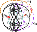
(b)

Figure 1: Illustration of an instance $\langle G(V,S),E,\Psi\rangle$ of SPB with $\omega=2$, where $G$ is a $2$-connected graph, $E=\{e_{i}:1\leq i\leq 5\}$, and $\Psi(e_{i})=i$. Solid edges belong to $G$. (a) and (b) show different embeddings of $G$ and assignments of the edges in $E$ to the faces of such embeddings. (a) determines a ${2}$-SDB of $\langle G(V,S),E,\Psi\rangle$, while (b) does not.

3 Complexity

In the following we study the computational complexity of testing planarity of streamed graphs with and without a backbone graph. First, we show that SPB is $\mathcal{NP}$-complete, even when the backbone graph is a spanning tree and $\omega=2$. This implies that Sunflower SEFE is $\mathcal{NP}$-complete for an arbitrary number of input graphs, even if every graph contains at most $\xi=2$ exclusive edges. Second, we show that SP is $\mathcal{NP}$-complete even for a constant window size $\omega$. This also has connections to the fundamental Weak Realizability Problem. Namely, Theorem 3.2 implies the $\mathcal{NP}$-completeness of Weak Realizability even for instances $\langle G(V,E),R\rangle$ such that the maximum number of occurrences $\theta$ of each edge of $E$ in the pairs of edges in $R$ is bounded by a constant, i.e., for each edge there is only a constant number $\theta$ of other edges it may not cross.

These results imply that, unless P=NP, no FPT algorithm with respect to $\omega$, to $\xi$, or to $\theta$ exists for Streamed Planarity (with Backbone), SEFE, and Weak Realizability Problems, respectively.

Theorem 3.1

SPB is $\mathcal{NP}$-complete for $\omega\geq 2$, even when the backbone graph is a tree and the edges of the stream form a matching.

Proof

The membership in $\mathcal{NP}$ follows from [11]. The $\mathcal{NP}$-hardness is proved by means of a polynomial-time reduction from problem Sunflower SEFE, which has been proved $\mathcal{NP}$-complete for $k=3$ graphs, even when the common graph is a tree $T$ and the exclusive edges of each graph only connect leaves of the tree [2].

Given an instance ${\langle G_{i}(V,E_{i})\rangle}^{3}_{i=1}$ of Sunflower SEFE, we construct a streamed graph $\langle G(V,S),E,\Psi\rangle$ that admits an $\omega$-SDB for $\omega=2$ if and only if ${\langle G_{i}(V,E_{i})\rangle}^{3}_{i=1}$ is a positive instance of Sunflower SEFE, as follows. To simplify the construction, we first replace instance ${\langle G_{i}(V,E_{i})\rangle}^{3}_{i=1}$ of Sunflower SEFE with an equivalent instance in which the exclusive edges in $E_{1}\cup E_{2}\cup E_{3}$ form a matching, by applying the technique described in [3]. Then, we perform the reduction starting from such a new instance. Refer to Fig. 2.

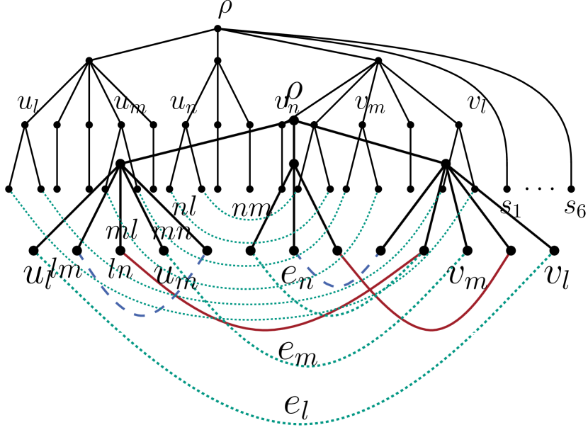
(a)

(b)

Figure 2: Illustration for the proof of Theorem 3.1. (a) Instance ${\langle G_{i}(V,E_{i})\rangle}^{3}_{i=1}$. (b) Partial representation of instance $\langle G(V,S),E,\Psi\rangle$ containing the edges of $G$ and the edges of the stream constructed starting from pairs of edges of $E_{3}$. Edges of $T$ and $G$ are black, edges of $G_{1}$, $G_{2}$, and $G_{3}$ are solid red, dashed blue, and dotted green, respectively.

First, set $G=T$. Then, for $i=1,2,3$ and for each edge $e=(u,v)\in E_{i}$, add to $G$ a star graph $S(u_{e})$ with leaves $u^{1}_{e},\dots,u^{q}_{e}$ and a star graph $S(v_{e})$ with leaves $v^{1}_{e},\dots,v^{q}_{e}$ with $q=|E_{i}|-1$, and identify the center of $S(u_{e})$ with $u$ and the center of $S(v_{e})$ with $v$, respectively. Also, consider the vertex $\rho$ of $G$ corresponding to any internal node of $T$, add to $G$ vertices $s_{i}$, for $i=1,\dots,6$ (sentinel leaves), and connect each of such vertices to $\rho$. Observe that, by construction, $G$ is a tree and $T\subset G$. The sentinel edges will serve as endpoints of edges of the stream, called sentinel edges, used to split the stream in three substreams in such a way that no edge of one substream is alive together with an edge of a different substream.

Further, set $E$ can be constructed as follows. For $i=1,2,3$ and for each pair $\langle l,m\rangle$ of edges in $E_{i}$, add to $E$ an edge $lm=(u^{a}_{l},v^{a}_{l})$ between a leaf of $S(u_{l})$ and a leaf of $S(v_{l})$ and an edge $ml=(u^{b}_{m},v^{b}_{m})$ between a leaf of $S(u_{m})$ and a leaf of $S(v_{m})$, respectively, for some $a,b\in{1,2,\dots,|E_{i}|-1}$, in such a way that no two edges in $E$ are incident to the same leaf of $G$. Observe that, by construction, $E$ is a matching. Also, add to $E$ edges $(s_{1},s_{2})$, $(s_{3},s_{4})$, and $(s_{5},s_{6})$ (sentinel edges).

Function $\Psi$ can be defined as follows. First, we construct an auxiliary ordering $\sigma=e_{h},\dots,e_{g}$ of the edges in $E$, then we just set $\Psi(e)=\sigma(e)$, for any edge $e\in E$, where $\sigma(e)$ denotes the position of $e$ in $\sigma$. To obtain $\sigma$, we consider sets $E_{1}$, $E_{2}$, and $E_{3}$ in this order and perform the following two steps. STEP 1: for each pair $\langle l,m\rangle$ of edges in $E_{i}$, add to $\sigma$ edge $lm$ and edge $ml$. STEP 2: add to $\sigma$ the sentinel edge $(v_{2(i-1)+1},u_{2(i-1)+2})$. Observe that, by construction, each common graph $G^{i}_{\cap}$ contains the edges of $G$ plus at most two edges $lm$ and $ml$ of the stream with $l,m\in E_{i}$, for some $i\in\{1,2,3\}$.

Observe that, the reduction can be easily performed in polynomial time.

We now shot that ${\langle G_{i}(V,E_{i})\rangle}^{3}_{i=1}$ admits a SEFE if and only if instance $\langle G(V,S),E,\Psi\rangle$ admits an $\omega$-SDB for $\omega=2$.

Suppose that ${\langle G_{i}(V,E_{i})\rangle}^{3}_{i=1}$ admits a SEFE ${\langle\mathcal{E}_{i}\rangle}^{3}_{i=1}$. Let $\mathcal{H}$ be the embedding of the common graph $T$ in ${\langle\mathcal{E}_{i}\rangle}^{3}_{i=1}$, that is, ${\mathcal{H}}=\mathcal{E}_{1}|_{T}=\mathcal{E}_{2}|_{T}=\mathcal{E}_{3}|_{T}$. We construct a planar embedding $\mathcal{E}$ of $G$ by defining the rotation scheme of each non-leaf vertex of $G$, as follows.

If $v$ is not a leaf of $T$, then the rotation scheme of $v$ in $\mathcal{E}$ is equal to the rotation scheme of $v$ in $\mathcal{H}$. If $v=u_{l}$ ($v=v_{l}$) is the unique neighbor of of any leaf vertex of $G$, then the rotation scheme of $u_{l}$ ($v_{l}$) can be chosen in such a way that the ordering of the leaves of $G$ that are adjacent to $u_{l}$ ($v_{l}$) is the reverse of the ordering of the leaves of $G$ that are adjacent to $v_{l}$ ($u_{l}$), where the the leaves of $G$ that are adjacent to $u_{l}$ ($v_{l}$) and to $v_{l}$ ($u_{l}$) are identified by the corresponding apex. We claim that the constructed embedding $\mathcal{E}$ of $G$ yields an $\omega$-SDB of $\langle G(V,S),E,\Psi\rangle$ for $\omega=2$. Let $\mathcal{O}$ be the circular ordering of the leaves of $T$ determined by an Eulerian tour of $T$ in $\mathcal{H}$. Also, let $\mathcal{O}^{\prime}$ be the circular ordering of the leaves of $G$ determined by an Eulerian tour of $G$ in $\mathcal{E}$. Suppose that there exist two edges $xy$ and $yx$ with $|\Psi(xy)-\Psi(yx)|<\omega=2$ such that the endpoints $u^{i}_{x}$ and $v^{i}_{x}$ of edge $xy$ and the endpoints $u^{j}_{y}$ and $v^{j}_{y}$ of edge $yx$ alternate in $\mathcal{O}^{\prime}$. This implies that the unique neighbors $u_{x}$ of $u^{i}_{x}$, $v_{x}$ of $v^{i}_{x}$, $u_{y}$ of $u^{j}_{y}$, and $v_{y}$ of $v^{j}_{y}$ in $T$ alternate in $\mathcal{O}$. This, in turn, implies a crossing between the two edges $x$ and $y$ of some set $E_{i}$. Hence, contradicting the fact that ${\langle\mathcal{E}_{i}\rangle}^{3}_{i=1}$ is a SEFE.

Suppose that $\langle G(V,S),E,\Psi\rangle$ admits an $\omega$-SDB for $\omega=2$. Let $\mathcal{E}$ be the planar embedding of $G$ in any $\omega$-SDB of $\langle G(V,S),E,\Psi\rangle$. Let $\mathcal{O}$ be the ordering of the leaves of $G$ in an Eulerian tour of $G$ in $\mathcal{E}$. Also, let $\mathcal{O}^{\prime}$ of the ordering of the leaves of $T$ in an Eulerian tour of $T$ in the embedding $H=\mathcal{E}|_{T}$. We claim that $H$ yields a SEFE of ${\langle G_{i}(V,E_{i})\rangle}^{3}_{i=1}$. Suppose that there exist two edges $x=(u_{x},v_{x})$ and $y=(u_{y},v_{y})$ of some set $E_{i}$ whose endpoints alternate in $\mathcal{O}^{\prime}$. Consider the two edges $xy=(u^{p}_{x},v^{p}_{x})$ and $yx=(u^{q}_{y},v^{q}_{y})$ of $E$, with $1\leq p\leq|E^{*}_{i}|-1$ and $1\leq q\leq|E^{*}_{i}|-1$. Since the sets of leaves of $S(u_{x})$, $S(v_{x})$, $S(u_{y})$, and $S(v_{y})$ appear in $\mathcal{O}$ in the same order as the vertices $u_{x}$, $v_{x}$, $u_{y}$, and $v_{y}$ appear in $\mathcal{O}^{\prime}$, the endpoints of $xy$ and $yx$ alternate in $\mathcal{O}^{\prime}$. Further, by construction, it holds that either $\Psi(xy)=\Psi(yx)+1$ or $\Psi(yx)=\Psi(xy)+1$, that is, either edge $xy$ immediately precedes edge $yx$ in the stream or edge $yx$ immediately precedes edge $xy$ in the stream. The above facts then imply a crossing between edge $xy$ and $yx$ of the stream. Hence, contradicting the hypothesis that $\langle G(V,S),E,\Psi\rangle$ admits an $\omega$-SDB for $\omega=2$.

The above discussion proves the statement for $\omega=2$. To extend the theorem to any value of $\omega\geq 2$ it suffices to augment $\langle G(V,S),E,\Psi\rangle$ with additional sentinel leaves and sentinel edges. This concludes the proof of the theorem.

Theorem 3.2

There is a constant $\omega_{0}$ such that deciding whether a given streamed graph is $\omega_{0}$-stream planar is $\mathcal{NP}$-complete.

Proof

The membership in $\mathcal{NP}$ follows from [11]. In the following we describe a reduction that, given a 3-SAT formula $\varphi$, produces a streamed graph that is $\omega_{0}$-stream planar if and only if $\varphi$ is satisfiable.

To make things simple, we do not describe the stream, but rather important keyframes. Our construction has the property that edges have a FIFO behavior, i.e., if edge $e$ appears before edge $f$, then also $e$ disappears before $f$. This, together with the fact that in each key frame only $O(1)$ edges are visible ensures that the construction can indeed be encoded as a stream with window size $O(1)$. The value $\omega_{0}$ we use is simply the maximum number of visible edges in any of the key frames. We do not take steps to further minimize $\omega_{0}$, but even without this, the value produced by the reduction is certainly less than 120, as we estimate at the end of the proof. Sometimes, we wish to wait until a certain set of edges has disappeared. In this case we insert sufficiently many isolated edges into the stream, which does not change the $\omega_{0}$-planarity of the stream.

We now sketch the construction. It consists of two main pieces. The first is a cage providing two faces called cells, one for vertices representing satisfied literals and one for vertices representing unsatisfied literals. We then present a clause stream for each clause of $\varphi$. It contains one literal vertex for each literal occurring in the clause and it ensures that these literal vertices are distributed to the two cells of the cage such that at least one goes in the cell for satisfied literals. Throughout we ensure that none of the previously distributed vertices leaves the respective cell.

Second, we present a sequence of edges that is $\omega_{0}$-stream planar if and only if the previously chosen distribution of the literal vertices forms a truth assignment. This is the case if and only if any two vertices representing the same literal are in the same cell and any two vertices representing complementary literals of one variable are in distinct cells.

It is clear that, if the constructions work as described, then the resulting streamed graph is $\omega_{0}$-stream planar if and only if $\varphi$ is satisfiable. The first part of the stream ensure that from each clause one of the literals must be assigned to the cell containing satisfied literals (i.e. the literal receives the value true). The second part ensures that these choices are consistent over all literals, i.e., these choices actually correspond to a truth assignment of the variables.

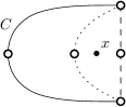
Figure 3: Cycle $C$ (solid and dashed edges) contains vertex $x$ in its interior. The dashed edges leave the sliding window soon. Presenting a new path (dotted) parallel to the old path does not ensure that $x$ ends up in the interior of the resulting cycle $C^{\prime}$ (solid and dotted edges).

Our first step will be the construction of the cage containing the two cells. Since the cage needs to persist throughout the whole sequence, it must be constructed in such a way that it can be “kept alive” over time by presenting new edges. Note that it does not suffice to repeatedly present edges that are parallel to existing ones, as they may be embedded differently, and hence over time allow isolated vertices to move through obstacles; see Fig. 3. We first present a construction that behaves like an edge that can be “renewed” without changing its drawing too much. We call it persistent edge.

(a)

(b)

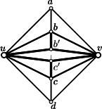
(c)

Figure 4: A persistent edge. The thickness of the edges indicates how long the edge stays in the sliding window. The thinner the edge the earlier it leaves the window. (a) The initial configuration; the dashed edge $bc$ dissolves first. It is used only once to initially enforce a unique planar embedding. (b) New vertices $b^{\prime}$ and $c^{\prime}$ with neighbors $u,b,v$ and $u,c,v$, respectively, are introduced. Starting from the embedding in (a) the embedding is uniquely defined. (c) After the edges incident to $a$ and $d$ disappear, the drawing has again the same structure as in (a). Repeating this cycle hence preserves the edge. Since edges are embedded only in the interior of the gadget vertices that are embedded outside the persistent edge cannot traverse it.

Let $u$ and $v$ be two vertices. A persistent edge between $u$ and $v$ consists of the four vertices $a,b,c,d$, each lying on a path of length 2 from $u$ to $v$. Additionally, $a$ is connected to $b$ and $b$ is connected to $c$. Initially, we also have insert the edge $b,c$ to enforce a unique planar embedding. However, once it leaves the sliding window it does not get replaced. Figure 4(a) shows a persistent edge where the thickness of the edge visualizes the time until an edge leaves the sliding window. The thicker the edge the longer it stays. Once the edge $bc$ has been removed, but before any of the other edges disappear, we present in the stream the edges $ub^{\prime}$, $vb^{\prime}$ and $bb^{\prime}$ as well as $uc^{\prime}$, $vc^{\prime}$ and $cc^{\prime}$, where $b^{\prime}$ and $c^{\prime}$ are new vertices; see Fig. 4(b). Note that there is a unique way to embed them into the given drawing. After the edges $ua$, $av$ leave the sliding window, $b$ takes over the role of $a$ and $b^{\prime}$ takes over the role of $b$. Similarly, after the edges $ud$ and $dv$ leave the sliding window, $c$ takes over the role of $d$ and $c^{\prime}$ takes over the role of $c$; see Fig. 4(c). By presenting six new edges in regular intervals, the persistent edge essentially keeps its structure. In particular, we know at any point in time which vertices are incident to the inner and outer face. For simplicity we will not describe in detail when to perform this book keeping. Rather, we just assume that the sliding window is sufficiently large to allow regular book keeping. For example, before each of the steps described later, we might first update all persistent edges, then present the gadget performing one of the steps, then update the persistent edges gain, and finally wait for the gadget edges to be removed from the sliding window again.

(a)

(b)

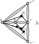
(c)

Figure 5: (a) The cage, the thick gray edges are persistent edges and are refreshed at regular intervals. After presenting all clause sequences, the faces $f^{+}$ and $f^{-}$ will contain the literal vertices corresponding to satisfied and unsatisfied literal vertices, respectively. (b) Edges used to check whether two literal vertices $x_{i}$ and $x_{j}$ are in the same face. (c) Edges used to check whether literal vertices $\overline{x_{i}}$ and $x_{j}$ are in distinct faces.

Next, we describe the cage. Conceptually, it consists of two cycles of length 4, on vertices $a,b,c,v^{+}$ and $a,b,c,v^{-}$, respectively. However, the edges are actually persistent edges; see Fig. 5(a). The interior faces $f^{+}$ and $f^{-}$ of the two cycles are the positive and negative literal faces, respectively. Note that at any point in time only a constant number of edges are necessary for the cage.

Before we describe the clause gadget, which is the most involved part of the construction, we briefly show how to perform the test for the end of sequence. Namely, assume that we have a set $V^{\prime}\subseteq V$ of literal vertices, and each of them is contained in one of the two literal faces. More formally, for each clause $c_{i}\in\varphi$ and for each Boolean variable $x$, set $V^{\prime}$ contains a literal vertex $x_{i}$, if $x\in c_{i}$, or a literal vertex $\overline{x_{i}}$, if $\overline{x}\in c_{i}$. To check whether two literal vertices $x_{i}$ and $x_{j}$ corresponding to a variable $x$ are in the same face, it suffices to present an edge between them in the stream, then wait until that edge leaves the sliding window, and continue with the next pair; see Fig 5(b). Of course, in the meantime we may have to refresh the persistent edges. Similarly, if we wish to check that literal vertices $\overline{x_{i}}$ and $x_{j}$ are in distinct faces, we make use of the fact that the two cycles forming the cage share two edges, and hence three vertices $a,b$ and $c$. We present in the stream the complete bipartite graph on the vertices $\{\overline{x_{i}},x_{j}\}$ and $\{a,b,c\}$. Clearly, this can be drawn in a planar way if and only if $\overline{x_{i}}$ and $x_{j}$ are in distinct faces; see Fig. 5(c). Again, it may be necessary to wait until these edges leave the sliding window before the next test can be performed.

(a)

(b)

(c)

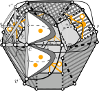
(d)

(e)

Figure 6: Illustration of the clause sequence. (a) Initial embedding of the clause. (b), (c) faces indicator vertices can reach if they are embedded in the face close to the center and close to the boundary, respectively. (d), separating the vertices corresponding to satisfied and unsatisfied literals into two distinct faces. (e) Integrating the now separated literal vertices into the corresponding faces of the cage.

Finally, we describe our clause gadget; see Fig. 6 for an illustration. First, we present the clause gadget as it is shown in Fig. 6(a). The literal vertices are large and solid, their corresponding indicator vertices are represented by large empty disks. The edges are ordered in the stream such that the three edges connecting a literal vertex to its indicator are presented first, i.e., they also leave the sliding window first. The remaining three edges incident to the literals are drawn last so that they remain present longest. Observe that the embedding of the clause without the literal and indicator vertices is unique; we call this part of the clause the frame. Each literal vertex may choose among two possible faces of the frame where it can be embedded. Either close to the center or close to the boundary. The faces in the center are shaded light gray, the faces on the boundary are shaded or tiled in a darker gray in Fig. 6(a).

We now first wait until the edges between literal vertices and their indicators leave the sliding window. Now the following things happen. First, the thin dotted and dashed edges leave the sliding window. Immediately afterwards, we present in the stream paths of length 2 that replace these edges, so the frame essentially remains as it is shown. However, after this step, the indicator vertex of any literal that was embedded in the face close to the center may be in any of the faces shaded in light gray in Fig. 6(b). Now, first the thick dotted edges leave the sliding window and are immediately replaced by parallel paths. Afterwards, the thick dashed edges leave the sliding window and are immediately replaced by parallel paths. Again, the frame remains essentially present. This allows the indicator vertices of literals that were embedded on the outer face to traverse into the faces indicated in Fig. 6(c). Note that, if all literal vertices were embedded in the face close the boundary, then there is no face of the frame that can simultaneously contain them at this point. If however, at least one of them was embedded in the face close to the center, then there is at least one face of the frame that can contain all the vertices simultaneously. We now include in the stream a triangle on the three indicator vertices. This triangle can be drawn without crossing edges of the frame if and only if the three vertices can meet in one face, which is the case if and only if at least one indicator vertex, and hence also its corresponding literal vertex, was embedded close to the center. Now we wait until the edges of the clause, except for those incident to the literal vertices and the paths that were renewed have vanished; see Fig. 6(d).

Let now $p$ be a new vertex, and denote the neighbors of the literal vertex $x$ by $\alpha_{x},\beta_{x}$ and $\gamma_{x}$, and similarly for $y$ and $z$. We now connect $v$ to the cage by present the edges $v^{-}v$ and $v^{+}v$ as well as edges forming a path from $c$ to $p$ that, starting from $p$, first visits $\alpha_{x},\beta_{x},\gamma_{x}$, then $\alpha_{y},\beta_{y},\gamma_{y}$, and finally $\alpha_{z},\beta_{z},\gamma_{z}$. Observe that the fact that $p$ has disjoint paths to $v^{-},v+$ and $v$ containing the $\alpha_{h},\beta_{h}$ and $\gamma_{h}$, with $h\in\{x,y,z\}$, ensures that, what remains of the clause gadget must be (and hence must have been all the time) embedded in the outer face of the cage. We assume without loss of generality that the path containing the $\alpha_{h},\beta_{h}$ and $\gamma_{h}$, with $h\in\{x,y,z\}$, is not incident to the outer face. Again, we consider the edges incident to the literal vertices not as part of the construction. Then the path is incident to precisely two faces, which are adjacent to the literal faces of the cage. Denote the one incident to $f_{+}$ by $f_{+}^{\prime}$ and the one incident to $f_{-}$ by $f_{-}^{\prime}$; see Fig. 6(d). Due to the traversal, we have that a literal vertex $v$ is contained in $f_{+}^{\prime}$ if and only if it was embedded in the face close to the center in the clause, which means that the corresponding literal was satisfied. Otherwise, it is embedded in $f_{-}^{\prime}$. It now remains to enclose the literal vertices into the corresponding face of the cage without letting escape any of the literal vertices already embedded there.

First, we wait until all edges incident to the literal vertices have left the sliding window, i.e., they become isolated. Then, we present two new persistent edges parallel to the existing persistent edges $v^{+}c$ and $v^{-}c$, respectively; see Fig. 6(e), where the new persistent edges are shaded dark gray. To ensure that the embedded is indeed as shown in Fig. 6(e), we one boundary vertex of each new persistent edge to a vertex on the outer boundary of the persistent edge it is parallel to (dashed lines in Fig. 6(e)). The new parallel edges replace the old persistent edges of the cage, and we wait until they have dissolved. Clearly, no vertex from an internal face of the cage can escape as the new persistent edges are embedded in the outer face of the cage. To ensure that the literal vertices must indeed be embedded in the literal faces, we present the edges $bx$, $by$ and $bz$. Finally, we wait until these edges vanish again. Then we are ready for the next clause sequence or for the final checking sequence.

The above description produces for a given 3SAT formula $\varphi$ produces, for a sufficiently large (but constant!) $\omega_{0}$ a stream $S_{\varphi}$ one some vertex set $V_{\varphi}$ such that $\varphi$ is satisfiable if and only if $S_{\varphi}$ is $\omega_{0}$-stream planar. In the first part of the stream, in any sequence of corresponding planar embedding, the literals of each clause, represented by vertices, are transferred to two interior faces of the cage such that for each clause at least one literal vertex is transferred to the face representing satisfied literals. This models the fact that each clause must contain at least one satisfied literal. In the second part, a sequence of edges is presented that is $\omega_{0}$-planar if and only if the previously produced distribution of literals to the positive and negative faces of the cage corresponds to a truth assignment of the underlying variables. The construction can clearly be performed in polynomial time.

We now briefly estimate the window size $\omega_{0}$. The largest number of edges that are simultaneously important in our construction occurs when presenting a clause gadget. A clause gadget has 48 edges, and it is simultaneously visible with four persistent edges, each of which may use up to 16 edges immediately after they have refreshed. Hence a window size of $\omega_{0}=112$ suffices for the construction.

4 Algorithms for $\omega$-Stream Drawings with Backbone

In this section, we describe a polynomial-time decision algorithm for the case that the backbone graph consists of a $2$-connected component plus, possibly, isolated vertices with no edge of the stream connecting two isolated vertices. We call instances satisfying these properties star instances, as the isolated vertices are the centers of edge disjoint star subgraphs of the union graph (see Section 4.1). Observe that, the requirement of the absence of edges of the stream between the isolated vertices of a star instance seems to be quite a natural restriction. In fact, as proved in Theorem 3.2, dropping this restriction makes the Streamed Planarity Problem computationally tough. This algorithm will also serve as a subprocedure to solve the SPB Problem for $\omega=1$ with no restrictions on the backbone graph (see Section 4.2).

4.1 Star Instances

In this section we describe an efficient algorithm to test the existence of an $\omega$-SDB for star instances (see Fig. 7(a)).

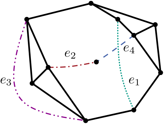
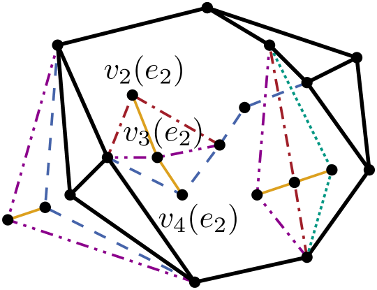
Figure 7: (a) A star instance with stream edges $E=\{e_{i}:1\leq i\leq 4\}$, $\Psi(e_{i})=i$, and $\omega=3$. (b) A SEFE of the instance of Sunflower SEFE obtained as described in Lemma 1 where $G_{\cup}$ is drawn with thick solid black edges, exclusive edges of $G_{i}$ are drawn with the same style as edge $e_{i}$ and exclusive edges of $G_{m+1}=G_{5}$ are drawn as yellow solid curves. Vertices in $D(e_{2})=\{v_{2}(e_{2}),v_{3}(e_{2}),v_{4}(e_{2})\}$ are also shown.

The problem is equivalent to finding an embedding $\mathcal{E}$ of the unique non-trivial $2$-connected component $\beta$ of $G$ and an assignment of the edges of the stream and of the isolated vertices of $G$ to the faces of $\mathcal{E}$ that yield a $\omega$-SDB.

Lemma 1

Let $\langle G(V,S),E,\Psi\rangle$ be a star instance of SPB and let $\omega$ be a positive integer window size. There exists an equivalent instance ${\langle G_{i}(V,E_{i})\rangle}^{m+1}_{i=1}$ of Sunflower SEFE such that the common graph $G_{\cap}$ consists of disjoint $2$-connected components. Further, instance ${\langle G_{i}(V,E_{i})\rangle}^{m+1}_{i=1}$ can be constructed in $O(n+\omega{}m)$ time.

Proof

Given a star instance $\langle G(V,S),E,\Psi\rangle$ of SPB we construct an instance ${\langle G_{i}(V,E_{i})\rangle}^{m+1}_{i=1}$ of Sunflower SEFE that admits a SEFE if and only if $\langle G(V,S),E,\Psi\rangle$ admits an $\omega$-SDB, as follows. Refer to Figs 7(a) and  7(b) for an example of the construction.

Initialize graph $G_{\cap}$ to the backbone graph $G$. Also, for every edge $e\in E$, add to $G_{\cap}$ a set of vertices $D(e)=\{v_{i}(e)\mid\Psi(e)\leq i<\min(\Psi(e)+\omega,m+1)\}$. Observe that, since $\langle G(V,S),E,\Psi\rangle$ is a star instance, graph $G_{\cap}$ contains a single non-trivial $2$-connected component $\beta$, plus a set of trivial $2$-connected components consisting of the isolated vertices in $\mathcal{Q}\cup\bigcup_{e\in E}D(e)$.

For $i=1,\dots,m$, graph $G_{i}$ contains all the edges and the vertices of $G_{\cap}$ plus a set of edges defines as follows. For each edge $e=(u,v)\in E$ such that $0\leq i-\Psi(e)<\omega$, add to $E(G_{i})$ edges $(u,v_{i}(e))$ and $(v_{i}(e),v)$. From a high-level view, graphs $G_{i}$, with $i=1,\dots,m$, are defined in such a way to enforce the same constraints on the possible embeddings of the common graph as the constraints enforced by the edges of the stream on the possible embeddings of the backbone graph.

Finally, graph $G_{m+1}$ contains all the edges and the vertices of $G_{\cap}$ plus a set of edges defined as follows. For each edge $e\in E$, add to $E_{m+1}$ edges $(v_{\Psi(e)}(e),v_{k}(e))$, with $\Psi(e)<k<min(\Psi(e)+\omega,m+1)$. Observe that, in any planar drawing $\Gamma_{m+1}$ of $G_{m+1}$, vertices $v_{k}(e)$ lie inside the same face of $\Gamma_{m+1}$, for any edge $e\in E$. The aim of graph $G_{m+1}$ is to combine the constrains imposed on the embedding of the backbone graph by each graph $G_{i}$, with $i=1,\dots,m$, in such a way that, for each edge $e\in E$, the edges of set $D(e)$ are embedded in the same face of the backbone graph.

Hereinafter, given a positive instance ${\langle G_{i}(V,E_{i})\rangle}^{m+1}_{i=1}$ of SEFE with the above properties, we denote the corresponding SEFE $\langle\Gamma_{i}\rangle^{m+1}_{i=1}$ by ${\langle\mathcal{E}_{i},A_{i}\rangle}^{m+1}_{i=1}$, where $\mathcal{E}_{i}$ represents the embedding of $\beta$ in $\Gamma_{i}$ and $A_{\mathcal{E}_{i}}$ represents the assignment of the isolated vertices and of the exclusive edges of graph $G_{i}$ in $\Gamma_{i}$ to the faces of $\mathcal{E}_{i}$, for $i=1,\dots,m+1$. Similarly, given a positive star instance $\langle G(V,S),E,\Psi\rangle$ of SPB we denote the corresponding $\omega$-SDB $\Gamma$ by $\langle\mathcal{E},A_{\mathcal{E}}\rangle$, where $\mathcal{E}$ represents the embedding of the unique non-trivial $2$-connected component $\beta$ of $G$ in $\Gamma$ and $A_{\mathcal{E}}$ represents the assignment of the isolated vertices of $G$ and of the edges of the stream to the faces of $\mathcal{E}$ in $\Gamma$. More formally, $A_{\mathcal{E}}\colon E\cup\mathcal{Q}\rightarrow F(\mathcal{E})$, where $F(\mathcal{E})$ denotes the set of facial cycles of $\mathcal{E}$.

Suppose that ${\langle G_{i}(V,E_{i})\rangle}^{m+1}_{i=1}$ is a positive instance of SEFE, that is, ${\langle G_{i}(V,E_{i})\rangle}^{m+1}_{i=1}$ admits a SEFE ${\langle\mathcal{E}_{i},A_{i}\rangle}^{m+1}_{i=1}$. We show how to construct a solution $\langle\mathcal{E},A_{\mathcal{E}}\rangle$ of $\langle G(V,S),E,\Psi\rangle$.

Since ${\langle\mathcal{E}_{i},A_{i}\rangle}^{m+1}_{i=1}$ is a SEFE and $\beta\in G_{\cap}$, we have that $\mathcal{E}_{i}=\mathcal{E}_{j}$, with $1\leq i<j\leq m+1$. We set the embedding $\mathcal{E}$ of $\beta$ to $\mathcal{E}_{1}$.

Further, for every edge $e\in E$, we set $A_{\mathcal{E}}(e)$ to the face of $\mathcal{E}_{1}$ vertex $v_{\Psi(e)}(e)$ is placed inside in $\Gamma_{1}$, that is, $A_{\mathcal{E}}(e)=A_{\mathcal{E}_{1}}(v_{\Psi(e)}(e))$. Similarly, for every isolated vertex $v\in\mathcal{Q}$, we set $A_{\mathcal{E}}(v)$ to the face of $\mathcal{E}_{1}$ vertex $v$ is placed inside in $\Gamma_{1}$, that is, $A_{\mathcal{E}}(v)=A_{\mathcal{E}_{1}}(v)$.

We need to prove that $\mathcal{E}$ is a planar embedding of $\beta$ and that no crossing occurs neither between an edge in $E$ and an edge in $\beta$ nor between two edges $e_{i}\in E$ and $e_{j}\in E$, with $i<j$ and $\Psi(e_{j})-\Psi(e_{i})<\omega$. Observe that, since ${\langle\mathcal{E}_{i},A_{i}\rangle}^{m+1}_{i=1}$ is a SEFE, the embedding $\mathcal{E}_{i}$ of $\beta$ in $\Gamma_{i}$ is planar. As $\mathcal{E}$ coincides with $\mathcal{E}_{1}$, it follows that $\mathcal{E}$ is also planar. Assume that there exists a crossing between an edge $e\in E$ and an edge of $\beta$. This implies that there exists in $\Gamma_{\Psi(e)}$ a path $p^{*}=(u,v_{\Psi(e)}(e),v)$ connecting two vertices of $u$ and $v$ of $\beta$ that are incident to different faces of $\mathcal{E}_{\Psi(e)}$. Further, assume that there exists a crossing between an edge $e_{i}\in E$ and an edge $e_{j}\in E$ with $\Psi(e_{i})<\Psi(e_{j})$ such that $\Psi(e_{j})-\Psi(e_{i})<\omega$ inside the same face $f$ of $\mathcal{E}$. This implies that there exists in $G_{\Psi(e_{i})}$ a crossing between a path $p^{\prime}=(a,\dots,v_{\Psi(e_{i})}(e_{i}),\dots,b)$ and $p^{\prime\prime}=(c,\dots,v_{\Psi(e_{i})}(e_{j}),\dots,d)$ only containing exclusive edges of $G_{\Psi(e_{i})}$ such that $a,c,b$, and $d$ apper in this order in the face of $\mathcal{E}_{\Psi(e_{i})}$ corresponding to $f$. Thus, both assumptions contradict the fact that $\langle G(V,S),E,\Psi\rangle$ admits an $\omega$-SDB.

Suppose that $\langle G(V,S),E,\Psi\rangle$ admits an $\omega$-SDB, that is, there exist a planar embedding $\mathcal{E}$ of $\beta$ and an assignment function $A_{\mathcal{E}}:E\cup\mathcal{Q}\rightarrow F(\mathcal{E})$ such that, for any two paths $p^{\prime}=(a,\dots,b)$ and $p^{\prime\prime}=(c,\dots,d)$ with $\{a,b,c,d\}\in\beta$ and $\Psi(e_{j})-\Psi(e_{i})<\omega$, for every edge $e_{i}\in p^{\prime}$ and $e_{j}\in p^{\prime\prime}$ with $i<j$, it holds that $A_{\mathcal{E}}(e_{i})\neq A_{\mathcal{E}}(e_{j})$. We show how to construct a SEFE ${\langle\mathcal{E}_{i},A_{i}\rangle}^{m+1}_{i=1}$ of ${\langle G_{i}(V,E_{i})\rangle}^{m+1}_{i=1}$.

For $i=1,\dots,m+1$, we set the embedding $\mathcal{E}_{i}$ of $\beta$ to $\mathcal{E}$. For $i=1,\dots,m+1$ and for each edge $e\in E$, we assign each vertex $v_{k}(e)\in D(e)$ to the face of $\mathcal{E}_{i}$ that corresponds to the face of $\mathcal{E}$ edge $e$ is assigned to, that is, $A_{\mathcal{E}_{i}}(v_{k}(e))=A_{\mathcal{E}}(e)$. Also, for each edge $e=(u,v)\in E$, we assign edges $(u,v_{k}(e))$ and $(v_{k}(e),v)$ to face $A_{\mathcal{E}_{k}}(v_{k}(e))$, with $\Psi(e)\leq k<min(\Psi(e)+\omega,m+1)$. Further, for each edge $e=(u,v)\in E$, we assign edges $(v_{\Psi(e)},v_{k}(e))$ to face $A_{\mathcal{E}_{m+1}}(v_{k}(e))$, with $\Psi(e)<k<min(\Psi(e)+\omega,m+1)$. Finally, for $i=1,\dots,m+1$ and for each vertex $v\in\mathcal{Q}$, we set $A_{\mathcal{E}_{i}}(v)=A_{\mathcal{E}}(v)$.

In order to prove that ${\langle\mathcal{E}_{i},A_{i}\rangle}^{m+1}_{i=1}$ is a SEFE of ${\langle G_{i}(V,E_{i})\rangle}^{m+1}_{i=1}$ we show that (i) $\mathcal{E}_{i}$ is a planar embedding of $\beta\in G_{i}$ (ii) all embeddings $\mathcal{E}_{i}$ coincide, (ii) there exists no crossing in $\Gamma_{i}$ involving the exclusive edges of any graph $G_{i}$, and (iv) each isolated vertex $v$ of $G_{\cap}$ is such that $A_{\mathcal{E}_{i}}(v)=A_{\mathcal{E}_{j}}(v)$, with $i\neq j$. Since $\mathcal{E}$ is planar by hypothesis and since $\mathcal{E}_{i}=\mathcal{E}$, condition (i) is trivially verified. Further, by construction, conditions (ii) and (iv), are also satisfied. Assume that condition (iii) does not hold. In this case, either an exclusive edge $(v_{i}(e),w)$ of $G_{i}$ crosses an edge of $\beta$ or there exists a crossing between two exclusive edges $(v_{i}(e_{1}),p)$ and $(v_{i}(e_{2}),q)$ of $G_{i}$ inside the same face of $\mathcal{E}_{i}$. In the former case, there must exists in $G_{i}$ a path $p_{0}=(a,v_{i}(e),b)$ composed of exclusive edges of $G_{i}$ connecting two vertices ${a,b}\in\beta$ (not necessarily different from $w$) that lie on the boundary of different faces of $\mathcal{E}_{i}$. However, this would imply that $G_{\cup}$ contains a path $p^{*}_{0}=(a,\dots,b)$ containing edge $e$ and only consisting of edges $e_{k}$ with $0\leq i-\Psi(e_{k})<\omega$, whose endpoints $a$ and $b$ lie on different faces of $\mathcal{E}$. In the latter case, there must exist two vertex-disjoint paths $p_{1}=(a,\dots,v_{i}(e_{1}),\dots,b)$ and $p_{2}=(c,\dots,v_{i}(e_{2}),\dots,d)$ of exclusive edges of $G_{i}$ contained in a face $f$ of $\mathcal{E}_{i}$ connecting vertices ${a,b}\in f$ and ${c,d}\in f$, respectively, such that $a,c,b$, and $d$ appear in this order along $f$. However, this would imply that $G_{\cup}$ contains two paths $p^{*}_{1}=(a,\dots,b)$ and $p^{*}_{2}=(c,\dots,d)$ with endpoints in $\beta$ containing edges $e_{1}$ and $e_{2}$, respectively, and only containing edges $e_{k}$ in $E$ with $0\leq i-\Psi(e_{k})<\omega$ that lie inside the face $f^{*}$ of $\mathcal{E}$ corresponding to face $f$ of $\mathcal{E}_{i}$ and whose endpoints alternate along the boundary of $f^{*}$. Thus, both assumptions contradict the fact that $\langle G(V,S),E,\Psi\rangle$ admits an $\omega$-SDB.

It is easy to see that instance ${\langle G_{i}(V,E_{i})\rangle}^{m+1}_{i=1}$ can be constructed in time $O(n+\omega{}m)$. In fact, the construction of the common graph $G_{\cap}$ takes $O(n)$-time, since the backbone graph $G$ is planar. Also, each graph $G_{i}$ can be encoded as the union of a pointer to the encoding of $G_{\cap}$ and of the encoding of its exclusive edges. Further, each graph $G_{i}$, with $i=1,\dots,m$, has at most $\omega$ exclusive edges, and graph $G_{m+1}$ has at most $\omega{}m$ exclusive edges. This concludes the proof of the lemma.

Lemma 1 provides a straight-forward technique to decide whether a star istance $\langle G(V,S),E,\Psi\rangle$ of SPB admits a $\omega$-SDB. First, transform instance $\langle G(V,S),E,\Psi\rangle$ into an equivalent instance ${\langle G_{i}(V,E_{i})\rangle}^{m+1}_{i=1}$ of SEFE of $m+1$ graphs with sunflower intersection and such that the common graph consists of disjoint $2$-connected components, by applying the reduction described in the proof of Lemma 1. Then, apply to instance ${\langle G_{i}(V,E_{i})\rangle}^{m+1}_{i=1}$ the algorithm by Bläsius et al. [5] that tests instances of SEFE with the above properties in linear time. Thus, we obtain the following theorem.

Theorem 4.1

Let $\langle G(V,S),E,\Psi\rangle$ be an star instance of SPB. There exists an $O(n+\omega{}m)$-time algorithm to decide whether $\langle G(V,S),E,\Psi\rangle$ admits an $\omega$-SDB.

4.2 Unit window size

In this section we describe a polynomial-time algorithm to test whether an instance $\langle G(V,S),E,\Psi\rangle$ of SPB admits an $\omega$-SDB for $\omega=1$. Observe that, in the case in which $\omega=1$, the SPB Problem equals to the problem of deciding whether an embedding of the backbone graph exists such that the endpoints of each edge of the stream lie on the boundary of the same face of such an embedding.

Let $\mathcal{G}_{1},\dots,\mathcal{G}_{1(G)}$ be the connected components of the backbone graph $G$. Given an embedding $\mathcal{E}$ of $G$, we define the set $F(\mathcal{E})$ of facial cycles of $\mathcal{E}$ as the union of the facial cycles of the embeddings $\mathcal{E}_{i}=\mathcal{E}|_{\mathcal{G}_{i}}$ of each connected component $\mathcal{G}_{i}$ of $G$ in $\mathcal{E}$. We first prove an auxiliary lemma which allows us to focus our attention only on instances whose backbone graph contains at most one non-trivial connected component.

Lemma 2

Let $\langle G(V,S),E,\Psi\rangle$ be an instance of SPB. There exists a set of instances $\langle G(V_{i},S_{i}),E_{i},\Psi_{i}\rangle$ whose backbone graph $G(V_{i},S_{i})$ contains at most one non-trivial connected component $\mathcal{G}_{i}$ such that $\langle G(V,S),E,\Psi\rangle$ admits a $\omega$-SDB with $\omega=1$ if and only if all instances $\langle G(V_{i},S_{i}),E_{i},\Psi_{i}\rangle$ admit a $\omega$-SDB with $\omega=1$. Further, such instances can be constructed in $O(n+m)$ time.

Proof

We construct instances $\langle G(V_{i},S_{i}),E_{i},\Psi_{i}\rangle$ starting from $G_{\cup}$ in two steps. To ease the description, we assume that each vertex $v\in V$ is initially associated with an index $l(v)$ corresponding to the connected component of $G$ vertex $v$ belongs to, that is, $l(v)=i$ if $v\in V(\mathcal{G}_{i})$. First, we recursively contract each edge $(u,v)$ of $G_{\cup}$ with $\{u,v\}\subseteq V(\mathcal{G}_{i})$ to a single vertex $w$ and set $l(w)=i$, for $i=1,\dots,1(G)$. Thus, obtaining an auxiliary graph $H$ on $1(G)$ vertices. Then, we obtain instances $\langle G(V_{i},S_{i}),E_{i},\Psi_{i}\rangle$ from $H$ by recursively uncontracting each vertex $w$ with $l(w)=i$, for $i=1,\dots,1(G)$. Note that, by construction, $\mathcal{G}_{i}\subseteq G(V_{i},S_{i})$.

Observe that, the construction of $H$ requires $O(n+m)$ time. Further, the construction of each instance $\langle G(V_{i},S_{i}),E_{i},\Psi_{i}\rangle$ can be performed in $O(n_{i}+m_{i})$ time, where $n_{i}=|V(\mathcal{G}_{i})|$ and $m_{i}$ is the number of edges in $E$ that are incident to a vertex of $G_{i}$, which sums up to $O(n+m)$ time in total for all $1\leq i\leq 1(G)$. Thus, proving the $O(n+m)$ running time of the construction.

The necessity is trivial. In order to prove the sufficiency, assume that all instances $\langle G(V_{i},S_{i}),E_{i},\Psi_{i}\rangle$ admit a $\omega$-SDB for $\omega=1$. Intuitively, a ${1}$-SDB $\Gamma$ of the original instance can be obtained, starting from a ${1}$-SDB $\Gamma_{i}$ of any $\langle G(V_{i},S_{i}),E_{i},\Psi_{i}\rangle$, by recursively replacing the drawing of each isolated vertex $v_{j}\in\mathcal{Q}_{i}$ with the ${1}$-SDB $\Gamma_{j}$ of $\langle G(V_{j},S_{j}),E_{j},\Psi_{j}\rangle$ (after, possibly, promoting a different face to be the outer face of $\Gamma_{j}$) . For a complete example, see Fig. 9. The fact that $\Gamma$ is a ${1}$-SDB of $\langle G(V,S),E,\Psi\rangle$ derives from the fact that each $\Gamma_{i}$ is a ${1}$-SDB of $\langle G(V_{i},S_{i}),E_{i},\Psi_{i}\rangle$, that in a ${1}$-SDB crossings among edges in $E$ do not matter, and that, by the connectivity of the union graph, the assignment of the isolated vertices in $\mathcal{Q}_{i}$ to the faces of the embedding $\mathcal{E}_{i}$ of $\mathcal{G}_{i}$ in $\Gamma_{i}$ must be such that any two isolated vertices connected by a path of edges of the stream $E_{i}$ lie inside the same face of $\mathcal{E}_{i}$. In the following, we prove this direction more formally.

We denote by $(\mathcal{E}_{i},C_{\mathcal{E}_{i}})$ the solution of instance $\langle G(V_{i},S_{i}),E_{i},\Psi_{i}\rangle$, where $\mathcal{E}_{i}$ is a planar embedding of $\mathcal{G}_{i}$ and $C_{\mathcal{E}_{i}}:F(\mathcal{E}_{i})\rightarrow 2^{\mathcal{Q}_{i}}$ is an assignment of the set of isolated vertices $\mathcal{Q}_{i}$ of $G(V_{i},S_{i})$ to the set of faces of $\mathcal{E}_{i}$, denoted by $F({\mathcal{E}_{i}})$. We now show how to extend the solutions $(\mathcal{E}_{i},C_{\mathcal{E}_{i}})$ of instances $\langle G(V_{i},S_{i}),E_{i},\Psi_{i}\rangle$, with $i=1,\dots,1(G)$, to a solution $\langle\mathcal{E},C_{\mathcal{E}}\rangle$ of instance $\langle G(V,S),E,\Psi\rangle$, where $\mathcal{E}$ is a planar embedding of $G$ defining the set of facial cycles and $C_{\mathcal{E}}:F(\mathcal{E})\rightarrow 2^{\{1,\dots,1(G)\}}$ is an assignment of the connected components of $G$ to the faces of $\mathcal{E}$.

To obtain $\mathcal{E}$, we set the rotation scheme of each vertex $v$ of $G$ in $\mathcal{E}$ to the rotation scheme of $v$ in the embedding $\mathcal{E}_{i}$ of the component $\mathcal{G}_{i}$ of the backbone graph $G$ containing $v$. Clearly, the set of facial cycles $F(\mathcal{E})$ of $\mathcal{E}$ is equal to the union of the set of facial cycles of each $\mathcal{E}_{i}$, that is, for each face $f\in\mathcal{E}$, we have that $f$ belongs to $\mathcal{E}_{i}$ for some $1\leq i\leq 1(\mathcal{G})$.

The assignment function $C_{\mathcal{E}}$ can be defined as follows. Initialize $C_{\mathcal{E}}(f)=\emptyset$, for each facial cycle $f$ in $F(\mathcal{E})$. Then, consider each pair of connected components $\mathcal{G}_{i}$ and $\mathcal{G}_{j}$ of the backbone graph and, for each facial cycle $f$ in $F(\mathcal{E})\cap F(\mathcal{E}_{j})$, set $C_{\mathcal{E}}(f)=C_{\mathcal{E}}(f)\cup i$ if $i\in C_{\mathcal{E}_{j}}(f)$.

We now prove that $(\mathcal{E},C_{\mathcal{E}})$ is a solution for $\langle G(V,S),E,\Psi\rangle$. Since each $\mathcal{E}_{i}$ is a planar embedding, then $\mathcal{E}$ is also planar. We just need to prove that for every two faces $f^{\prime}$ and $f^{\prime\prime}$ of $\mathcal{E}$ either (i) $C_{\mathcal{E}}(f^{\prime})\subseteq C_{\mathcal{E}}(f^{\prime\prime})$, or (ii) $C_{\mathcal{E}}(f^{\prime\prime})\subseteq C_{\mathcal{E}}(f^{\prime})$, or (iii) $C_{\mathcal{E}}(f^{\prime})\cap C_{\mathcal{E}}(f^{\prime\prime})=\emptyset$. Clearly, if $f^{\prime},f^{\prime\prime}\in\mathcal{E}_{i}$ for some $i$, exactly one of (i), (ii), and (iii) must hold, as otherwise $(\mathcal{E}_{i},C_{\mathcal{E}_{i}})$ would not be a solution of $\langle G(V_{i},S_{i}),E_{i},\Psi_{i}\rangle$. We prove that there exist no $f^{\prime}\in\mathcal{E}_{i}$ and $f^{\prime\prime}\in\mathcal{E}_{j}$ with $i\neq j$ such that neither (i), (ii), or (iii) holds. We distinguish three cases according to whether $j\in C_{\mathcal{E}_{i}}(f^{\prime})$, or $i\in C_{\mathcal{E}_{j}}(f^{\prime\prime})$, or $j\notin C_{\mathcal{E}_{i}}(f^{\prime})\wedge i\notin C_{\mathcal{E}_{j}}(f^{\prime\prime})$. By the connectivity of the union graphs of each instance and by the fact that $(\mathcal{E}_{i},C_{\mathcal{E}_{i}})$ and $(\mathcal{E}_{j},C_{\mathcal{E}_{j}})$ are $\omega$-SDB of $\langle G(V_{i},S_{i}),E_{i},\Psi_{i}\rangle$ and $\langle G(V_{j},S_{j}),E_{j},\Psi_{j}\rangle$, respectively, we have that: (i) must hold, if $i\in C_{\mathcal{E}_{j}}(f^{\prime\prime})$; (ii) must hold, if $j\in C_{\mathcal{E}_{i}}(f^{\prime})$; and (iii) must hold, if $j\notin C_{\mathcal{E}_{i}}(f^{\prime})\wedge i\notin C_{\mathcal{E}_{j}}(f^{\prime\prime})$. This concludes the proof of the lemma.

By Lemma 2, in the following we only consider the case in which the backbone graph consists of a single non-trivial connected component plus, possibly, isolated vertices. We now present a simple recursive algorithm to test instances with this property.

Algorithm ALGOCON.

• an instace $I=$ $\langle G(V,S),E,\Psi\rangle$ of the SPB Problem with $\omega=1$ with union graph $G_{\cup}$ such that $G$ contains at most one non-trivial connected component.

• YES, if $\langle G(V,S),E,\Psi\rangle$ is positive, or NO, otherwise.

BASE CASE 1: instance $I$ is such that $2(G)=0$, that is, every connected component of $G$ is an isolated vertex. Return YES, as instances of this kind are trivially positive.

BASE CASE 2: instance $I$ is such that (i) $2(G)=1$, that is, the backbone graph $G$ consists of a single $2$-connected component plus, possibly, isolated vertices and (ii) no edge of the stream connects any two isolated vertices. In this case, apply the algorithm of Theorem 4.1 to decide $I$ and return YES, if the test succeeds, or NO, otherwise.

RECURSIVE STEP: instance $I$ is such that either (CASE R1) $2(G)=1$ and there exists edges of the stream between pairs of isolated vertices or (CASE R2) $2(G)>1$. First, replace instance $I$ with two smaller instances $I^{\diamond}=$ $\langle G(V_{\diamond},S_{\diamond}),E_{\diamond},\Psi_{\diamond}\rangle$ and $I^{\circ}=$ $\langle G(V_{\circ},S_{\circ}),E_{\circ},\Psi_{\circ}\rangle$, as described below. Then, return YES, if ${\sc ALGOCON}(I^{\diamond})=$ ${\sc ALGOCON}(I^{\circ})$ $=$ YES, or NO, otherwise.

• Instance $I^{\diamond}$ is obtained from $I$ by recursively contracting every edge $(u,v)$ of $G_{\cup}$ with $\{u,v\}\nsubseteq V(\mathcal{G})$. Instance $I^{\circ}$ is obtained from $I$ by recursively contracting every edge $(u,v)$ of $G_{\cup}$ with $\{u,v\}\subseteq V(\mathcal{G})$.

• Let $\mathcal{G}$ be the unique non-trivial connected component of $G$, let $T$ be the block-cutvertex tree of $\mathcal{G}$ rooted at any block, and let $\beta$ be any leaf block in $T$. Also, let $v$ be the parent cutvertex of $\beta$ in $T$. We first construct an auxiliary equivalent instance $I^{*}=$ $\langle G(V_{*},S_{*}),E_{*},\Psi_{*}\rangle$ starting from $I$ and then obtain instances $I^{\diamond}$ and $I^{\circ}$ from $I^{*}$, as follows. See Fig. 8 for an illustration of the construction of instance $I^{*}$.

  

  

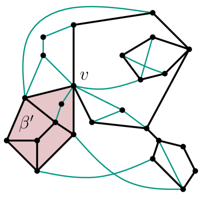
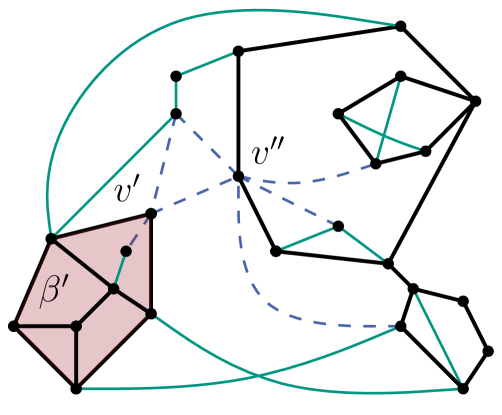
  Figure 8: (a) Instance $I$ and (b) instance $I^{*}$ obtained in CASE R2 of Algorithm ALGOCON. Edges of the backbone graph are black thick curves; edge of the stream are green thin curves; and edges of the stream incident to $v^{\prime}$ and $v^{\prime\prime}$ in $I^{*}$ are blue dashed curves.

  Initialize $I^{*}$ to $I$. Replace vertex $v$ in $V_{*}$ with two vertices $v^{\prime}$ and $v^{\prime\prime}$ and make (i) $v^{\prime}$ adjacent to all the vertices of $\beta$ vertex $v$ used to be adjacent to and (ii) $v^{\prime\prime}$ adjacent to all the vertices in $V(\mathcal{G})\setminus V(\beta)$ vertex $v$ used to be adjacent to. Then, replace each edge $(v,x)$ of $E^{*}$ with edge $(v^{\prime},x)$, if $x\in V(\beta)$ or if $x\in\mathcal{Q}^{*}$ and there exists a path composed of edges of the stream connecting $x$ to a vertex $y\neq v\in V(\beta)$, and edge $(v^{\prime\prime},x)$, if $x\in V(\mathcal{G})\setminus V(\beta)$ or if $x\in\mathcal{Q}^{*}$ and there exists a path composed of edges of the stream connecting $x$ to a vertex $y\neq v\in V(\mathcal{G})\setminus V(\beta)$. Finally, add edge $(v^{\prime},v^{\prime\prime})$ to $E^{*}$. It is easy to see that instances $I$ and $I^{*}$ are equivalent.

  Instance $I^{\diamond}$ is obtained from $I^{*}$ by recursively contracting every edge $(u,v)$ of $G^{*}_{\cup}$ with $u,v\nsubseteq V(\beta)$, where $G^{*}_{\cup}$ is the union graph of $I^{*}$. Instance $I^{\circ}$ is obtained from $I^{*}$ by recursively contracting every edge $(u,v)$ of $G^{*}_{\cup}$ with $\{u,v\}\subseteq V(\beta)$.

Theorem 4.2

Let $\langle G(V,S),E,\Psi\rangle$ be an instance of SPB. There exists an $O(n+m)$-time algorithm to decide whether $\langle G(V,S),E,\Psi\rangle$ admits an $\omega$-SDB for $\omega=1$.

Proof

The algorithm runs in two steps, as follows.

• STEP 1 applies the reduction illustrated in the proof of Lemma 2 to $\langle G(V,S),E,\Psi\rangle$ to construct $1(G)$ instances $\langle G(V_{i},S_{i}),E_{i},\Psi_{i}\rangle$ such that the backbone graphs $G(V_{i},S_{i})$ contain at most one non-trivial connected component.

• STEP 2 applies Algorithm ALGOCON to every instance $\langle G(V_{i},S_{i}),E_{i},\Psi_{i}\rangle$ and return YES, if all such instances are positive, or NO, otherwise.

Observe that, the correctness of the presented algorithm follows from the correctness of Lemma 2, of Theorem 4.1, and of Algorithm ALGOCON. We now prove the correctness for Algorithm ALGOCON. Obviously, the fact that instances $I^{\diamond}$ and $I^{\circ}$ constructed in CASE R1 and CASE R2 are both positive is a necessary and sufficient condition for instance $I$ to be positive. We prove termination by induction on the number $2(G)$ of blocks of the backbone graph $G$ of instance $I$, primarily, and on the number of edges of the stream connecting isolated vertices of the backbone graph, secondarily. (i) If $2(G)=0$, then BASE CASE 1 applies and the algorithm stops; (ii) if $2(G)=1$ and no two isolated vertices of the backbone graph are connected by an edge of the stream, then BASE CASE 2 applies and the algorithm stops; (iii) if $2(G)=1$ and there exist edges of the stream between any two isolated vertices of the backbone graph $G$, then, by CASE R1, instance $I$ is split into (a) an instance $I^{\diamond}$ with $2(G(V_{\diamond},E_{\diamond}))=1$ and no edges of the stream connecting any two isolated vertices of the backbone graph $G(V_{\diamond},E_{\diamond})$, and (b) an instance $I^{\circ}$ with $2(G(V_{\circ},E_{\circ}))=0$; (iv) finally, if $2(G)>1$, then, by CASE R2, instance $I$ is split into (a) an instance $I^{\circ}$ with $2(G(V_{\diamond},E_{\diamond}))=1$ and (b) an instance $I^{\circ}$ with $2(G(V_{\circ},E_{\circ}))=2(G)-1$.

The running time easily derives from the fact that all instances $\langle G(V_{i},S_{i}),E_{i},\Psi_{i}\rangle$ can be constructed in $O(n+m)$-time and that the algorithm for star instances described in the proof of Theorem 4.1 runs in $O(n+\omega{}m)$-time. This concludes the proof.

Acknowledgments.

Giordano Da Lozzo was supported by the MIUR project AMANDA “Algorithmics for MAssive and Networked DAta”, prot. 2012C4E3KT_001. Ignaz Rutter was supported by a fellowship within the Postdoc-Program of the German Academic Exchange Service (DAAD). This work was done while the authors where visiting the Department of Applied Mathematics at Charles University in Prague.

(a)

(b)

(c)

(d)

(e)

(f)

(g)

(h)

(i)

(j)

(k)

(l)

Figure 9: (a) Instance $I=$ $\langle G(V,S),E,\Psi\rangle$ of SPB with $\omega=1$, where $G$ consists of $4$ connected components $\mathcal{G}_{1}$, $\mathcal{G}_{2}$, $\mathcal{G}_{3}$, and $\mathcal{G}_{4}$. Edges of the backbone graph are black thick curves. Edges of the stream are green thin curves. Instances $I_{1}$ (b), $I_{2}$ (d), $I_{3}$ (f), and $I_{4}$ (h) obtained by applying the procedure described in the proof of Lemma 2 to instance $I$. ${1}$-SDB $\Gamma_{1}$ (c), $\Gamma_{2}$ (e), $I_{3}$ (g), and $I_{4}$ (i) of instances $I_{1}$, $I_{2}$, $I_{3}$, and $I_{4}$, respectively. (j) ${1}$-SDB $\Gamma^{12}$ obtained by replacing the drawing of $\mathcal{G}_{2}$ in $\Gamma_{1}$ with $\Gamma_{2}$. (k) ${1}$-SDB $\Gamma^{123}$ obtained by replacing the drawing of $\mathcal{G}_{3}$ in $\Gamma^{12}$ with $\Gamma^{3}$. (l) ${1}$-SDB $\Gamma^{1234}$ obtained by replacing the drawing of $\mathcal{G}_{4}$ in $\Gamma^{123}$ with $\Gamma_{4}$.

References

- [1] Angelini, P., Binucci, C., Da Lozzo, G., Didimo, W., Grilli, L., Montecchiani, F., Patrignani, M., Tollis", I.: Drawing non-planar graphs with crossing-free subgraphs. In: Wismath, S., Wolff, A. (eds.) Graph Drawing (GD ’13). LNCS, vol. 8242, pp. 295–307 (2013)
- [2] Angelini, P., Da Lozzo, G., Neuwirth, D.: Advancements on SEFE and partitioned book embedding problems. Theoretical Computer Science (2014), in Press
- [3] Angelini, P., Di Battista, G., Frati, F., Patrignani, M., Rutter, I.: Testing the simultaneous embeddability of two graphs whose intersection is a biconnected or a connected graph. J. Discrete Algorithms 14, 150–172 (2012)
- [4] Bläsius, T., Kobourov, S.G., Rutter, I.: Simultaneous embedding of planar graphs. In: Tamassia, R. (ed.) Handbook of Graph Drawing and Visualization. CRC Press (2013)
- [5] Bläsius, T., Karrer, A., Rutter, I.: Simultaneous embedding: Edge orderings, relative positions, cutvertices. In: Wismath, S.K., Wolff, A. (eds.) Graph Drawing (GD ’13). LNCS, vol. 8242, pp. 220–231 (2013)
- [6] Brandes, C.B.U., Di Battista, G., Didimo, W., Gaertler, M., Palladino, P., Patrignani, M., Symvonis, A., Zweig, K.A.: Drawing trees in a streaming model. Inf. Process. Lett. 112(11), 418–422 (2012)
- [7] Di Battista, G., Eades, P., Tamassia, R., Tollis, I.G.: Graph Drawing. Upper Saddle River, NJ (1999)
- [8] Di Battista, G., Tamassia, R.: On-line planarity testing. SIAM J. Comput. 25(5), 956–997 (1996)
- [9] Gassner, E., Jünger, M., Percan, M., Schaefer, M., Schulz, M.: Simultaneous graph embeddings with fixed edges. In: WG ’06. pp. 325–335 (2006)
- [10] Schaefer, M.: Picking planar edges; or, drawing a graph with a planar subgraph. In: Duncan, C.A., Symvonis, A. (eds.) Graph Drawing (GD ’14). LNCS, vol. 8871, pp. 13–24 (2014)
- [11] Schaefer, M., Sedgwick, E., Stefankovic, D.: Recognizing string graphs in NP. J. Comput. Syst. Sci. 67(2), 365–380 (2003)