Maximal $\bf L^{p}$ analysis of finite element solutions for parabolic equations with
nonsmooth coefficients in convex polyhedra

Abstract.

The paper is concerned with Galerkin finite element solutions of parabolic equations in a convex polygon or polyhedron with a diffusion coefficient in $W^{1,N+\alpha}$ for some $\alpha>0$, where $N$ denotes the dimension of the domain. We prove the analyticity of the semigroup generated by the discrete elliptic operator, the discrete maximal $L^{p}$ regularity and the optimal $L^{p}$ error estimate of the finite element solution for the parabolic equation.

1. Introduction

Let $\Omega$ be a bounded domain in $\mathbb{R}^{N}$ (with $N=2$ or $N=3$), and let $S_{h}$ be a finite element subspace of $H^{1}_{0}(\Omega)$ consisting of continuous piecewise polynomials of degree $r\geq 1$ subject to certain quasi-uniform triangulation of the domain $\Omega$. We consider the parabolic equation

(1.4) $$\left\{\begin{array}[]{ll}\partial_{t}u-\nabla\cdot(a\nabla u)=f&\mbox{in}~{}~{}\Omega\times(0,\infty),\\ \displaystyle u=0&\mbox{on}~{}~{}\partial\Omega\times(0,\infty),\\ u(\cdot,0)=u^{0}&\mbox{in}~{}~{}\Omega,\end{array}\right.$$

and its finite element approximation

(1.7) $$\left\{\begin{array}[]{ll}\big{(}\partial_{t}u_{h},v_{h}\big{)}+(a\nabla u_{h},\nabla v_{h})=(f,v_{h}),~{}~{}\forall~{}v_{h}\in S_{h},\\ u_{h}(0)=u^{0}_{h},\end{array}\right.$$

where $f$ is a given function, and $a=(a_{ij}(x))_{N\times N}$ is an $N\times N$ symmetric matrix which satisfies the ellipticity condition

(1.8) $$\Lambda^{-1}|\xi|^{2}\leq\sum_{i,j=1}^{N}a_{ij}(x)\xi_{i}\xi_{j}\leq\Lambda|\xi|^{2},\quad\mbox{for}~{}~{}x\in\Omega,$$

for some positive constant $\Lambda$.

If we define the elliptic operator $A:H^{1}_{0}(\Omega)\rightarrow H^{-1}(\Omega)$ and its finite element approximation $A_{h}:S_{h}\rightarrow S_{h}$ by

(1.9) $$(Aw,v):=(a\nabla w,\nabla v),\qquad\qquad\,\,\forall~{}w,v\in H^{1}_{0}(\Omega),$$

(1.10) $$(A_{h}w_{h},v_{h}):=(a\nabla w_{h},\nabla v_{h}),\qquad\forall~{}w_{h},v_{h}\in S_{h},$$

then the solutions of (1.4) and (1.7) can be expressed by

(1.11) $$u(t)=E(t)u^{0}+\int_{0}^{t}E(t-s)f(s){\rm d}s,$$

(1.12) $$u_{h}(t)=E_{h}(t)u^{0}_{h}+\int_{0}^{t}E_{h}(t-s)f(s){\rm d}s,$$

where $\{E(t)=e^{-tA}\}_{t>0}$ and $\{E_{h}(t)=e^{-tA_{h}}\}_{t>0}$ denote the semigroups generated by the operators $-A$ and $-A_{h}$, respectively. By the theory of parabolic equations and [33], it is well known that $\{E(t)\}_{t>0}$ is an analytic semigroup on $C_{0}(\overline{\Omega})$ satisfying

(1.13) $$\|E(t)v\|_{L^{\infty}}+t\|\partial_{t}E(t)v\|_{L^{\infty}}\leq C\|v\|_{L^{\infty}},\quad\forall\,v\in C_{0}(\overline{\Omega}),~{}\forall\,t>0,$$

which is equivalent to the resolvent estimate

$$\|(\lambda+A)^{-1}v\|_{L^{\infty}}\leq C\lambda^{-1}\|v\|_{L^{\infty}},\quad\forall\,v\in C_{0}(\overline{\Omega}),\,\,\forall\,\lambda\in\Sigma_{\theta+\pi/2},$$

where $\Sigma_{\theta+\pi/2}:=\{z\in\mathbb{C}:|{\rm arg}(z)|<\theta+\pi/2\}$. The counterparts of these two inequalities above for the discrete finite element operator $A_{h}$ are the analyticity of the semigroup $\{E_{h}(t)\}_{t>0}$ on $L^{\infty}\cap S_{h}$:

(1.14) $$\|E_{h}(t)v_{h}\|_{L^{\infty}}+t\|\partial_{t}E_{h}(t)v_{h}\|_{L^{\infty}}\leq C\|v_{h}\|_{L^{\infty}},\quad\forall\,v_{h}\in S_{h},\,\forall\,t>0,$$

and the resolvent estimate

$$\|(\lambda+A_{h})^{-1}v_{h}\|_{L^{\infty}}\leq C\lambda^{-1}\|v_{h}\|_{L^{\infty}},\quad\forall\,v_{h}\in S_{h},\,\,\forall\,\lambda\in\Sigma_{\varphi+\pi/2}.$$

The estimates of the discrete semigroup have attracted much attention in the past several decades. With these estimates, one may reach more precise analyses of finite element solutions, such as maximum-norm analysis of FEMs [31, 45, 46, 48], error estimates of fully discrete FEMs [30, 34, 45] and the discrete maximal $L^{p}$ regularity for parabolic finite element equations [14, 15, 22, 25, 27].

The proof of (1.14) dates back to Schatz et. al. [38], who proved (1.14) with a logarithmic factor for the heat equation in a two-dimensional smooth convex domain with the linear finite element method. The logarithmic factor was removed in the case $r\geq 4$ for $N=1,2,3$ in [32], and the analysis was further extended to the case $1\leq N\leq 5$ in [4]. Later, a unified approach was presented in [39] by Schatz et. al., where they proved (1.14) with the Neumann boundary condition for all $r\geq 1$ and $N\geq 1$. The result was extended to the Dirichlet boundary condition in [47] for the linear finite element method. Some other maximum-norm error estimates can be found in [7, 8, 11, 20, 24, 28], and the resolvent estimates can be found in [1, 2].

A related topic is the discrete maximal $L^{p}$ regularity (when $u^{0}=0$ and $1<p,q<\infty$)

(1.15) $$\|\partial_{t}u_{h}\|_{L^{p}((0,T);L^{q})}+\|A_{h}u_{h}\|_{L^{p}((0,T);L^{q})}\leq C_{p,q}\|f\|_{L^{p}((0,T);L^{q})},$$

which resembles the maximal $L^{p}$ regularity of the continuous parabolic problem and was proved by Geissert [14, 15]. A straightforward application of (1.15) is the $L^{p}$-norm error estimate

(1.16) $$\|P_{h}u-u_{h}\|_{L^{p}((0,T);L^{q})}\leq C_{p,q}(\|P_{h}u^{0}-u_{h}^{0}\|_{L^{q}}+\|P_{h}u-R_{h}u\|_{L^{p}((0,T);L^{q})}),$$

where $R_{h}$ is the Ritz projection associated with the operator $A$ and $P_{h}$ is the $L^{2}$ projection onto the finite element space.

All these estimates were established under the assumption that the coefficients $a_{ij}$ and the domain $\Omega$ are smooth enough so that the parabolic Green’s function satisfies

(1.17) $$|\partial_{t}^{\gamma}\partial_{x}^{\beta}G(t,x,y)|\leq C(t^{1/2}+|x-y|)^{-(N+2\gamma+|\beta|)}e^{-\frac{|x-y|^{2}}{Ct}},~{}~{}\forall~{}0\leq\gamma\leq 2,\,0\leq|\beta|\leq 2\,.$$

Although the condition on the coefficients was relaxed to $a_{ij}\in C^{2+\alpha}(\overline{\Omega})$ in [14], this assumption is still too strong for many physical applications. One of the examples is an incompressible miscible flow in porous media [9, 26], where the diffusion-dispersion tensor $[a_{ij}]_{i,j=1}^{N}$ is only a Lipschitz continuous function of the velocity field. In a recent work [25], the first author proved (1.14) in a smooth domain under the assumption $a_{ij}\in W^{1,\infty}(\Omega)$, together with the estimate (when $u^{0}=0$ and $1<p,q<\infty$)

(1.18) $$\|u_{h}\|_{L^{p}((0,T);W^{1,q})}\leq C_{p,q}\|f\|_{L^{p}((0,T);W^{-1,q})},$$

which were then applied to the incompressible miscible flow in porous media [27]. Moreover, the problem in a polygon or a polyhedron is of high interest in practical cases, while the inequality (1.17) does not hold in arbitrary convex polygons or polyhedra, and all the analyses of (1.15)-(1.18) are limited to smooth domains so far. For the problem in two-dimensional polygons with constant coefficients, the inequality (1.14) with an extra logarithmic factor was proved in [3, 35, 45] by using the following estimate of the discrete Green’s function $\Gamma_{h}$:

$$\int_{\Omega}|\Gamma_{h}(t,x,x_{0})|dx\leq C|\ln h|\,.$$

The corresponding results in three-dimensional polyhedra are unknown. More interested is whether these stability estimates hold with the natural regularity $a_{ij}\in W^{1,p}(\Omega)$ for some $1<p<\infty$, since such estimates are important for the extension of the analysis to a general nonlinear model.

This paper focuses on (1.14)-(1.15) and (1.18) in a convex polygon or polyhedron with a weaker regularity of the diffusion coefficient. Instead of estimating $\Gamma_{h}$ directly, we present a more precise estimate for the error function $F:=\Gamma_{h}-\Gamma$ (see Lemma 2.2) with which the logarithmic factor can be removed (this idea was used in [39]), where $\Gamma$ is a regularized Green’s function. To compensate the lack of pointwise estimate of the second-order derivatives of the Green’s function, we use local $W^{1,\infty}$ estimate and local energy estimates of the second-order derivatives (see Lemma 4.1). Our main result is the following theorem.

Theorem 1.1.

Assume that $a_{ij}\in W^{1,N+\alpha}(\Omega)$ for some $\alpha>0$, satisfying the condition (1.8), and assume that $\Omega$ is either a convex polygon in $\mathbb{R}^{2}$ or a convex polyhedron in $\mathbb{R}^{3}$. Then

(1) the semigroup estimate (1.14) holds,

(2) the solution of (1.7) satisfies (1.15) when $f\in L^{p}((0,T);L^{q})$ and $u^{0}=0$,

(3) the solution of (1.7) satisfies (1.18) when $f\in L^{p}((0,T);W^{-1,q})$ and $u^{0}=0$.

Under the assumptions in Theorem 1.1 and assuming that the solution of (1.4) satisfies $u\in C(\overline{\Omega}\times[0,T])$, (1.16) follows immediately from (1.15).

The rest of this paper is organized as follows. In section 2, we introduce some notations and present a key lemma based on which our main theorem can be proved. In section 3, we present superapproximation results for smoothly truncated finite element functions and present several estimates for the parabolic Green’s functions under the assumed regularity of the coefficients and the domain. Based on these estimates, we prove our key lemma in section 4.

2. Notations, assumptions and sketch of the proof

2.1. Notations

For any nonnegative integer $k$ and $1\leq p\leq\infty$, we let $W^{k,p}(\Omega)$ be the conventional Sobolev space of functions defined in $\Omega$, and let $W^{1,p}_{0}(\Omega)$ be the subspace of $W^{1,p}(\Omega)$ consisting of functions whose traces vanish on $\partial\Omega$. As conventions, we denote the dual space of $W^{1,p}_{0}(\Omega)$ by $W^{-1,p^{\prime}}(\Omega)$ for $1\leq p<\infty$, and denote $H^{k}(\Omega):=W^{k,2}(\Omega)$ and $L^{p}(\Omega):=W^{0,p}(\Omega)$ for any integer $k$ and $1\leq p\leq\infty$.

Let $Q_{T}:=\Omega\times(0,T)$. For any Banach space $X$ and a given $T>0$, we let $L^{p}((0,T);X)$ be the Bochner spaces equipped with the norm

$$\|f\|_{L^{p}((0,T);X)}=\left\{\begin{array}[]{ll}\displaystyle\biggl{(}\int_{0}^{T}\|f(t)\|_{X}^{p}dt\biggl{)}^{\frac{1}{p}},&1\leq p<\infty,\\[10.0pt] \displaystyle{\rm ess\,\,}\sup_{\!\!\!\!\!\!\!\!\!\!t\in(0,T)}\,\|f(t)\|_{X}.&p=\infty,\end{array}\right.$$

To simplify notations, in the following sections, we write $L^{p}$, $H^{k}$ and $W^{k,p}$ as the abbreviations of $L^{p}(\Omega)$, $H^{k}(\Omega)$ and $W^{k,p}(\Omega)$, respectively, and denote by $(\cdot\,,\cdot\,)$ the inner product in $L^{2}(\Omega)$. For any subdomain $Q\subset Q_{T}$, we define

$$Q^{t}:=\{x\in\Omega:~{}(x,t)\in Q\},$$

$$\|f\|_{L^{\infty,2}(Q)}:={\rm ess}\!\!\sup_{t\in(0,T)}\|f(\cdot,t)\|_{L^{2}(Q^{t})},$$

$$\|f\|_{L^{p}(Q)}:=\bigg{(}\iint_{Q}|f(x,t)|^{p}{\rm d}x{\rm d}t\bigg{)}^{\frac{1}{p}},\quad\forall\,1\leq p<\infty,$$

and denote $w(t)=w(\cdot,t)$ for any function $w$ defined on $Q_{T}$.

We assume that $\Omega$ is partitioned into quasi-uniform triangular elements $\tau_{l}^{h}$, $l=1,\cdots,L$, with $h=\max_{l}\{\mbox{diam}\,\tau_{l}^{h}\}$, and let $S_{h}$ be a finite element subspace of $H^{1}_{0}(\Omega)$ consisting of continuous piecewise polynomials of degree $r\geq 1$ subject to the triangulation. Let $a(x)=\left(a_{ij}(x)\right)_{N\times N}$ be the coefficient matrix and define the operators

$$A:H^{1}_{0}\rightarrow H^{-1},\qquad~{}\,A_{h}:S_{h}\rightarrow S_{h},$$

$$R_{h}:H^{1}_{0}\rightarrow S_{h},\qquad~{}~{}\,P_{h}:L^{2}\rightarrow S_{h},$$

by

$$\big{(}A\phi,v\big{)}=\big{(}a\nabla\phi,\nabla v\big{)} \mbox{for all~{}~{}$\phi,v\in H^{1}_{0}$},$$

$$\big{(}A_{h}\phi_{h},v\big{)}=\big{(}a\nabla\phi_{h},\nabla v\big{)} \mbox{for all~{}~{}$\phi_{h}\in S_{h}$, $v\in S_{h}$},$$

$$\big{(}A_{h}R_{h}w,v\big{)}=\big{(}Aw,v\big{)} \mbox{for all~{}~{}$w\in H^{1}_{0}$ and $v\in S_{h}$},$$

$$\big{(}P_{h}\phi,v\big{)}=\big{(}\phi,v\big{)} \mbox{for all~{}~{}$\phi\in L^{2}$ and $v\in S_{h}$}.$$

Clearly, $R_{h}$ is the Ritz projection operator associated to the elliptic operator $A$ and $P_{h}$ is the $L^{2}$ projection operator onto the finite element space. The following estimates are useful in this paper.

Lemma 2.1.

If $\Omega$ is a bounded convex domain and $a_{ij}\in W^{1,N+\alpha}(\Omega)$, $N\geq 2$, then we have

(2.1) $$\|w\|_{H^{2}}\leq C\|\nabla\cdot(a\nabla w)\|_{L^{2}}, \forall\,w\in H^{1}_{0},$$

(2.2) $$\|\nabla w\|_{L^{\infty}}\leq C_{p}\|\nabla\cdot(a\nabla w)\|_{L^{p}},\qquad\mbox{for any given $p>N$}, \forall\,w\in H^{1}_{0},$$

and the solution of (1.4) with $u^{0}=0$ satisfies

(2.3) $$\|\partial_{t}u\|_{L^{p}((0,T);L^{q})}+\|Au\|_{L^{p}((0,T);L^{q})}\leq C_{p,q}\|f\|_{L^{p}((0,T);L^{q})},$$

(2.4) $$\|\partial_{t}u\|_{L^{p}((0,T);W^{-1,q})}+\|u\|_{L^{p}((0,T);W^{1,q})}\leq C_{p,q}\|f\|_{L^{p}((0,T);W^{-1,q})},$$

for all $1<p,q<\infty$.

In the Lemma above, (2.1) is the standard $H^{2}$-regularity estimate in convex domains and (2.2) is a simple consequence of the Green’s function estimates given in Theorem 3.3–3.4 of [18], and (2.3)-(2.4) are consequences of the maximal $L^{p}$ regularity (see Appendix for details).

2.2. Properties of the finite element space and Green’s functions

For any subdomain $D\subset\Omega$, we denote by $S_{h}(D)$ the space of functions restricted to the domain $D$, and denote by $S_{h}^{0}(D)$ the subspace of $S_{h}(D)$ consisting of functions which equal zero outside $D$. For any given subset $D\subset\Omega$, we denote $B_{d}(D)=\{x\in\Omega:{\rm dist}(x,D)\leq d\}$ for $d>0$. Then there exist positive constants $K$ and $\kappa$ such that the triangulation and the corresponding finite element space $S_{h}$ possess the following properties ($K$ and $\kappa$ are independent of the subset $D$ and $h$).

(P0)  Quasi-uniformity:

For all triangles (or tetrahedron) $\tau_{l}^{h}$ in the partition, the diameter $h_{l}$ of $\tau_{l}^{h}$ and the radius $\rho_{l}$ of its inscribed ball satisfy

$$K^{-1}h\leq\rho_{l}\leq h_{l}\leq Kh.$$

(P1)  Inverse inequality:

If $D$ is a union of elements in the partition, then

$$\|\chi_{h}\|_{W^{l,p}(D)}\leq Kh^{-(l-k)-(N/q-N/p)}\|\chi_{h}\|_{W^{k,q}(D)},\quad\forall\,\,\chi_{h}\in S_{h},$$

for $0\leq k\leq l\leq 1$ and $1\leq q\leq p\leq\infty$.

(P2)  Local approximation and superapproximation:

(1) There exists a linear operator $I_{h}:H^{1}_{0}(\Omega)\rightarrow S_{h}$ such that if $d\geq\kappa h$, then

$$\|v-I_{h}v\|_{L^{2}(D)}\leq K\sum_{l=0}^{k}h^{k}d^{-l}\|v\|_{H^{{k-l}}(B_{d}(D))},\quad\forall\,\,v\in H^{k}\cap H^{1}_{0},\,\,\,1\leq k\leq 2.$$

Moreover, if supp$(v)\subset\overline{D}$, then $I_{h}v\in S_{h}^{0}(B_{d}(D))$. For example, the Clément interpolation operator defined in [5] has these properties. Also, the Lagrange interpolation operator $\Pi_{h}$ satisfies

$$\|v-\Pi_{h}v\|_{L^{2}(D)}+h\|\nabla(v-\Pi_{h}v)\|_{L^{2}(D)}\leq Kh^{2}\|\nabla^{2}v\|_{L^{2}(B_{d}(D))},\quad\forall\,\,v\in H^{2}\cap H^{1}_{0}.$$

(2) If $d\geq\kappa h$, $\omega=0$ outside $B_{2d}(D)$ and $|\partial^{\beta}\omega|\leq Cd^{-|\beta|}$ for all multi-index $\beta$, then for any $\psi_{h}\in S_{h}(B_{3d}(D))$ there exists $\eta_{h}\in S_{h}^{0}(B_{3d}(D))$ such that

$$\|\omega\psi_{h}-\eta_{h}\|_{H^{k}(B_{3d}(D))}\leq Kh^{1-k}d^{-1}\|\psi_{h}\|_{L^{2}(B_{3d}(D))},\quad k=0,1.$$

Furthermore, if $\omega\equiv 1$ on $B_{d}(D)$, then $\eta_{h}=\psi_{h}$ on $D$ and

$$\|\omega\psi_{h}-\eta_{h}\|_{H^{k}(B_{3d}(D))}\leq Kh^{1-k}d^{-1}\|\psi_{h}\|_{L^{2}(B_{3d}(D)\backslash D)},\quad k=0,1.$$

For example, $\eta_{h}=\Pi_{h}(\omega\psi_{h})$ has these properties.

(P3)  Regularized Delta function:

For any $x_{0}\in\overline{\tau}_{j}^{h}$, there exists a function $\widetilde{\delta}_{x_{0}}\in C^{3}(\overline{\Omega})$ with support in $\tau_{j}^{h}$ such that

$$\chi_{h}(x_{0})=\int_{\tau_{j}^{h}}\chi_{h}\widetilde{\delta}_{x_{0}}{\rm d}x,\quad\forall\,\chi_{h}\in S_{h},$$

$$\|\widetilde{\delta}_{x_{0}}\|_{W^{l,p}}\leq Kh^{-l-N(1-1/p)}\quad\mbox{for}\,\,\,1\leq p\leq\infty,\,\,\,l=0,1,2,3.$$

(P4)  Discrete Delta function

Let $\delta_{x_{0}}$ denote the Dirac Delta function centered at $x_{0}$, i.e. $\int_{\Omega}\delta_{x_{0}}(y)\varphi(y){\rm d}y=\varphi(x_{0})$ for any $\varphi\in C(\overline{\Omega})$. The discrete Delta function $P_{h}\widetilde{\delta}_{x_{0}}$ satisfies that

$$P_{h}\widetilde{\delta}_{x_{0}}(x)\leq Kh^{-N}e^{-\frac{|x-x_{0}|}{Kh}},\quad\forall\,x,x_{0}\in\Omega.$$

The properties (P0)-(P4) hold for any quasi-uniform partition with those standard finite element spaces and also, have been used in many previous works such as [25, 39, 41, 47]. The proof can be found in the appendix of [41].

For an element $\tau_{l}^{h}$ and a point $x_{0}\in\overline{\tau}_{l}^{h}$, we let $G(t,x,x_{0})$ be the Green’s function of the parabolic equation, defined by

(2.5) $$\partial_{t}G(t,\cdot,x_{0})+AG(t,\cdot,x_{0})=0\quad\mbox{for $t>0$ with $G(0,x,x_{0})=\delta_{x_{0}}(x)$},$$

The regularized Green’s function $\Gamma(t,x,x_{0})$ is defined by

(2.6) $$\partial_{t}\Gamma(\cdot,\cdot,x_{0})+A\Gamma(\cdot,\cdot,x_{0})=0\quad\mbox{for~{} $t>0$~{} with~{} $\Gamma(0,\cdot,x_{0})=\widetilde{\delta}_{x_{0}}$},$$

where $\widetilde{\delta}_{x_{0}}$ is given in (P2), and the discrete Green’s function $\Gamma_{h}(\cdot,\cdot,x_{0})$ is defined by

(2.7) $$\partial_{t}\Gamma_{h}(\cdot,\cdot,x_{0})+A_{h}\Gamma_{h}(\cdot,\cdot,x_{0})=0\quad\mbox{for~{} $t>0$~{} with~{} $\Gamma_{h}(0,\cdot,x_{0})=P_{h}\widetilde{\delta}_{x_{0}}$}.$$

The functions $G(t,x,x_{0})$ and $\Gamma_{h}(t,x,x_{0})$ are symmetric with respect to $x$ and $x_{0}$.

By the fundamental estimates of parabolic equations, there exists a positive constant $C$ such that ([12], Theorem 1.6; note that the Green’s function in the domain $\Omega$ is less than the Green’s function in $\mathbb{R}^{N}$)

(2.8) $$|G(t,x,y)|\leq C(t^{1/2}+|x-y|)^{-N}e^{-\frac{|x-y|^{2}}{Ct}}.$$

By estimating $\Gamma(t,x,x_{0})=\int_{\Omega}G(t,x,y)\widetilde{\delta}_{x_{0}}(y){\rm d}y$, it is easy to see that (2.8) also holds when $G$ is replaced by $\Gamma$ and when $\max(t^{1/2},|x-y|)\geq 2h$.

2.3. Decomposition of the domain $\Omega\times(0,T)$

Here we present some further notations on a dyadic decomposition of the domain $\Omega\times(0,T)$, which were introduced in [39] and also used in many other articles [14, 24, 25, 47]. Let $R_{0}$ be the smallest distance between a corner and a closed face which does not contained this corner.

For the given polygon/polyhedron $\Omega$, there exists a positive constant $K_{0}\geq\max(1,R_{0})$ (which depends on the interior angle of the edges/corners of $\Omega$) such that

(1) if $z_{0}$ is a point in the interior of $\Omega$ and $B_{\rho}(z_{0})$ intersects a face of $\Omega$, then $B_{\rho}(z_{0})\subset B_{2\rho}(z_{1})$ for some $z_{1}$ which is on a face of $\Omega$;

(2) if $z_{1}$ is on a face of $\Omega$ and $B_{\rho}(z_{1})$ intersects another face, then $B_{\rho}(z_{1})\subset B_{\rho K_{0}}(z_{2})$ for some $z_{2}$ which is on an edge of $\Omega$;

(3) if $z_{2}$ is on an edge of $\Omega$ and $B_{\rho}(z_{2})$ intersects another face which does not contain this edge, then $B_{\rho}(z_{2})\subset B_{\rho K_{0}}(z_{3})$ for some $z_{3}$ which is a corner of $\Omega$.

For any integer $j\geq 1$, we define $d_{j}=2^{-j-3}R_{0}K_{0}^{-2}$. For a given $x_{0}\in\Omega$, we let $J_{*}$ be an integer satisfying $d_{J_{*}}=2^{-J_{*}-3}R_{0}K_{0}^{-2}=C_{*}h$ with $C_{*}\geq\max(10,10\kappa,R_{0}K_{0}^{-2}/8)$ to be determined later. Thus, $J_{*}=\log_{2}[R_{0}K_{0}^{-2}/(8C_{*}h)]\leq\log_{2}(2+1/h)$ and $J_{*}>1$ when $h<R_{0}K_{0}^{-2}/(16C_{*})$. Let

$$Q_{*}(x_{0})=\{(x,t)\in\Omega_{T}:\max(|x-x_{0}|,t^{1/2})\leq d_{J_{*}}\},$$

$$\Omega_{*}(x_{0})=\{x\in\Omega:|x-x_{0}|\leq d_{J_{*}}\}\,,$$

$$Q_{j}(x_{0})=\{(x,t)\in\Omega_{T}:d_{j}\leq\max(|x-x_{0}|,t^{1/2})\leq 2d_{j}\},$$

$$\Omega_{j}(x_{0})=\{x\in\Omega:d_{j}\leq|x-x_{0}|\leq 2d_{j}\},$$

$$D_{j}(x_{0})=\{x\in\Omega:|x-x_{0}|\leq 2d_{j}\}$$

for $j\geq 1$; see Figure 1.

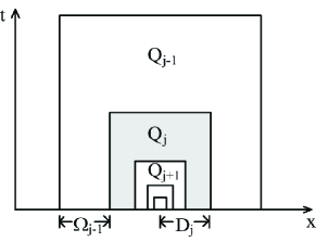
Figure 1. Illustration of the subdomains $Q_{j}$, $\Omega_{j}$ and $D_{j}$.

For $j=0$ we define $Q_{0}(x_{0})=Q_{T}\backslash Q_{1}(x_{0})$ and $\Omega_{0}(x_{0})=\Omega\backslash\Omega_{1}(x_{0})$, and for $j<0$ we simplify define $Q_{j}(x_{0})=\Omega_{j}(x_{0})=\emptyset$. For all $j\geq 1$ we define

$$\Omega_{j}^{\prime}(x_{0})=\Omega_{j-1}(x_{0})\cup\Omega_{j}(x_{0})\cup\Omega_{j+1}(x_{0}),$$

$$\Omega_{j}^{\prime\prime}(x_{0})=\Omega_{j-2}(x_{0})\cup\Omega_{j}^{\prime}(x_{0})\cup\Omega_{j+2}(x_{0}),$$

$$\Omega_{j}^{\prime\prime\prime}(x_{0})=\Omega_{j-2}(x_{0})\cup\Omega_{j}^{\prime\prime}(x_{0})\cup\Omega_{j+2}(x_{0}),$$

$$Q_{j}^{\prime}(x_{0})=Q_{j-1}(x_{0})\cup Q_{j}(x_{0})\cup Q_{j+1}(x_{0}),$$

$$Q_{j}^{\prime\prime}(x_{0})=Q_{j-2}(x_{0})\cup Q_{j}^{\prime}(x_{0})\cup Q_{j+2}(x_{0}),$$

$$Q_{j}^{\prime\prime\prime}(x_{0})=Q_{j-2}(x_{0})\cup Q_{j}^{\prime\prime}(x_{0})\cup Q_{j+2}(x_{0}),$$

$$D_{j}^{\prime}(x_{0})=D_{j-1}(x_{0})\cup D_{j}(x_{0}),$$

$$D_{j}^{\prime\prime}(x_{0})=D_{j-2}(x_{0})\cup D_{j}^{\prime}(x_{0}),$$

$$D_{j}^{\prime\prime\prime}(x_{0})=D_{j-3}(x_{0})\cup D_{j}^{\prime\prime}(x_{0}).$$

Then we have

$$\Omega_{T}=\bigcup^{J_{*}}_{j=0}Q_{j}(x_{0})\,\cup Q_{*}(x_{0})\quad\mbox{and}\quad\Omega=\bigcup^{J_{*}}_{j=0}\Omega_{j}(x_{0})\,\cup\Omega_{*}(x_{0}),$$

We refer to $Q_{*}(x_{0})$ as the “innermost” set. We shall write $\sum_{*,j}$ when the innermost set is included and $\sum_{j}$ when it is not. When $x_{0}$ is fixed, if there is no ambiguity, we simply write $Q_{j}=Q_{j}(x_{0})$, $Q_{j}^{\prime}=Q_{j}^{\prime}(x_{0})$, $Q_{j}^{\prime\prime}=Q_{j}^{\prime\prime}(x_{0})$, $\Omega_{j}=\Omega_{j}(x_{0})$, $\Omega_{j}^{\prime}=\Omega_{j}^{\prime}(x_{0})$ and $\Omega_{j}^{\prime\prime}=\Omega_{j}^{\prime\prime}(x_{0})$.

In the rest of this paper, we denote by $C$ a generic positive constant, which will be independent of $h$, $x_{0}$, and the undetermined constant $C_{*}$ until it is determined at the end of section 4.2.

2.4. Proof of Theorem 1.1

The keys to the proof of Theorem 1.1 are several more precise estimates of the Green’s functions. Let $F(t)=\Gamma_{h}(t)-\Gamma(t)$. Then for any $x_{0}\in\Omega$, we have

$$(E_{h}(t)v_{h})(x_{0}) =(F(t),v_{h})+(\Gamma(t),v_{h})$$

(2.9) $$=\int_{0}^{t}(\partial_{t}F(s),v_{h}){\rm d}s+(F(0),v_{h})+(\Gamma(t),v_{h}),$$

$$(t\partial_{t}E_{h}(t)v_{h})(x_{0}) =(t\partial_{t}F(t),v_{h})+(t\partial_{t}\Gamma(t),v_{h})$$

(2.10) $$=\int_{0}^{t}(s\partial_{ss}F(s)+\partial_{s}F(s),v_{h}){\rm d}s+(t\partial_{t}\Gamma(t),v_{h}),$$

with $\|F(0)\|_{L^{1}}=\|\widetilde{\delta}_{x_{0}}-P_{h}\widetilde{\delta}_{x_{0}}\|_{L^{1}}\leq C$ (according to (P3) and (P4)). Moreover, by the analyticity of the continuous parabolic semigroup on $L^{1}(\Omega)$, we have

$$\|\Gamma(t)\|_{L^{1}}+t\|\partial_{t}\Gamma(t)\|_{L^{1}}\leq C\|\Gamma(0)\|_{L^{1}}=C\|\widetilde{\delta}_{x_{0}}\|_{L^{1}}\leq C.$$

We present some estimates of these Green’s functions in the following lemma. The proof of the lemma is the major work of this paper and will be given in the next two sections.

Lemma 2.2.

Under the assumptions of Theorem 1.1, we have

(2.11) $$\int_{0}^{\infty}\int_{\Omega}\big{(}|\partial_{t}F(t,x,x_{0})\big{|}+\big{|}t\partial_{tt}F(t,x,x_{0})|\big{)}{\rm d}x{\rm d}t\leq C,$$

(2.12) $$|\nabla\partial_{t}G(t,x,x_{0})|\leq C\max(t^{1/2},|x-x_{0}|)^{-3-N}\quad\mbox{for}\,\,\,\,(x,t)\in\Omega\times(0,1).$$

The estimates in Lemma 2.2 were proved in [39] for parabolic equations with the Neumann boundary condition and in [47] for the Dirichlet boundary condition. However, their proofs are only valid for smooth coefficients and smooth domains (as clearly mentioned in their papers). Later, these estimates were proved in [25] for parabolic equations in smooth domains of arbitrary dimensions under the Neumann boundary condition with Lipschitz continuous coefficients. Here we are concerned with the problem in a convex polyhedron in two or three dimensional spaces under the Dirichlet boundary condition with $a_{ij}\in W^{1,N+\alpha}$.

Proof of Theorem 1.1: Firstly, from (2.9)-(2.10) we see that (1.14) is a consequence of (2.11).

Secondly, we can view $E_{h}(t)$ as an analytic semigroup on $L^{q}(\Omega)$, defined by

$$(E_{h}(t)v)(x_{0}):=\int_{\Omega}\Gamma_{h}(t,x,x_{0})v(x){\rm d}x,$$

whose generator is $A_{h}P_{h}$. From [49, Theorem 4.2] and [50, Lemma 4.c] (with a duality argument for the case $q\geq 2$) we know that the maximal $L^{p}$ regularity (1.15) holds if the following maximal ergodic estimate holds:

(2.13) $$\bigg{\|}\sup_{t>0}\frac{1}{t}\int_{0}^{t}|E_{h}(s)|\,v\,{\rm d}s\bigg{\|}_{L^{q}}\leq C\|v\|_{L^{q}},\quad\forall\,v\in L^{q}(\Omega),$$

where

$$(|E_{h}(s)|v)(x_{0}):=\int_{\Omega}|\Gamma_{h}(t,x,x_{0})|v(x){\rm d}x.$$

Let $G_{\rm tr}(t,x,x_{0})$ be a truncated Green’s function which is symmetric with respect to $x$ and $x_{0}$ and satisfies $G_{\rm tr}(t,x,x_{0})=G(t,x,x_{0})$ when $(x,t)$ is outside $Q_{*}(x_{0})$ (see [25, Section 4.2] on its construction). Then we have (assuming that $\tau_{0}^{h}$ is the triangle/tetrahedron which contains $x_{0}$)

$$\iint_{[\Omega\times(0,\infty)]\backslash Q_{*}(x_{0})}|\partial_{t}\Gamma(t,x,x_{0})-\partial_{t}G_{\rm tr}(t,x,x_{0})|{\rm d}x{\rm d}t$$

$$=\iint_{[\Omega\times(0,1)]\backslash Q_{*}(x_{0})}\biggl{|}\int_{\Omega}\partial_{t}G(t,x,y)\widetilde{\delta}_{x_{0}}(y){\rm d}y-\partial_{t}G(t,x,x_{0})\biggl{|}{\rm d}x{\rm d}t$$

$$\quad+\iint_{\Omega\times(1,\infty)}|\partial_{t}\Gamma(t,x,x_{0})-\partial_{t}G(t,x,x_{0})|{\rm d}x{\rm d}t$$

$$\leq Ch\iint_{[\Omega\times(0,1)]\backslash Q_{*}(x_{0})}\sup_{y\in\tau_{0}^{h}}\big{|}\nabla_{y}\partial_{t}G(t,x,y)\big{|}{\rm d}x{\rm d}t$$

$$\quad+C\int_{1}^{\infty}t^{-1}(\|\Gamma(t/2,\cdot,x_{0})\|_{L^{1}}+\|G(t/2,\cdot,x_{0})\|_{L^{1}}){\rm d}t\quad\mbox{[by semigroup estimate]}$$

$$=Ch\sum_{j}\iint_{Q_{j}(x_{0})}\sup_{(y,t)\in Q_{j}^{\prime}(x)}\big{|}\nabla_{y}\partial_{t}G(t,x,y)\big{|}{\rm d}x{\rm d}t+C\int_{1}^{\infty}t^{-1-N/2}{\rm d}t\quad\mbox{[see (\ref{FEstP})] }$$

$$\leq C\sum_{j}\frac{h}{d_{j}}+C\quad\mbox{[see (\ref{DxtGrEst})]}$$

$$\leq C.$$

By using energy estimates, it is easy to see

$$\iint_{Q_{*}(x_{0})}(|\partial_{t}\Gamma(t,x,x_{0})|+|\partial_{t}G_{\rm tr}(t,x,x_{0})|){\rm d}x{\rm d}t$$

$$\leq d_{J_{*}}^{N/2+1}(\|\partial_{t}\Gamma(\cdot,\cdot,x_{0})\|_{L^{2}(\Omega\times(0,1))}+\|\partial_{t}G_{\rm tr}(\cdot,\cdot,x_{0})\|_{L^{2}(\Omega\times(0,1))})\leq C_{*}^{N/2+1},$$

where the constant $C_{*}$ will be determined at the end of Section 4. Then (2.11) and the last two inequalities imply

$$\int_{0}^{\infty}\int_{\Omega}|\partial_{t}\Gamma_{h}(t,x,x_{0})-\partial_{t}G_{\rm tr}(t,x,x_{0})|{\rm d}x{\rm d}t\leq C.$$

In other words, the symmetric kernel $K(x,y):=\int_{0}^{\infty}|\partial_{t}\Gamma_{h}(t,x,y)-\partial_{t}G^{*}_{\rm tr}(t,x,y)|{\rm d}t$ satisfies

$$\sup_{y\in\Omega}\int_{\Omega}K(x,y){\rm d}x+\sup_{x\in\Omega}\int_{\Omega}K(x,y){\rm d}y\leq C,$$

and therefore, Schur’s lemma implies that the corresponding operator $M_{K}$, defined by $M_{K}{v}(x)=\int_{\Omega}K(x,y){v}(y){\rm d}y$, is bounded on $L^{q}(\Omega)$ for all $1\leq q\leq\infty$. Let $E^{*}_{\rm tr}(t){v}(x)=\int_{\Omega}G_{\rm tr}^{*}(t,x,y){v}(y){\rm d}y$ and note that $E^{*}_{\rm tr}(t){v}(x)\leq E(t)|{v}|(x)$ (because $G_{\rm tr}^{*}(t,x,y)\leq G(t,x,y)$). We have

$${\sup_{t>0}(|E_{h}(t)P_{h}|v)(x)}$$

$$\leq{\sup_{t>0}(|E_{h}(t)P_{h}|v-E^{*}_{\rm tr}(t)v)(x)+\sup_{t>0}(E^{*}_{\rm tr}(t)v)(x)}$$

$$\leq{\sup_{t>0}\big{(}|E_{h}(t)P_{h}-E^{*}_{\rm tr}(t)|\,|v|\big{)}(x)+\sup_{t>0}(E^{*}_{\rm tr}(t)v)(x)}$$

$$={\sup_{t>0}\bigg{|}(|P_{h}\widetilde{\delta}_{x}|,|v|)+\int_{0}^{t}\int_{\Omega}|\partial_{t}\Gamma_{h}(s,x,y)-\partial_{t}G^{*}_{\rm tr}(s,x,y)|\,|v(y)|{\rm d}y{\rm d}s\bigg{|}}$$

$$\quad+{\sup_{t>0}(E^{*}_{\rm tr}(t)|v|)(x)}$$

$$\leq{(|P_{h}\widetilde{\delta}_{x}|,|v|)+(M_{K}|v|)(x)+\sup_{t>0}(E(t)|v|)(x)}$$

where

$${\|\sup_{t>0}E(t)|v|\|_{L^{q}}\leq C_{q}\|v\|_{L^{q}},}\quad\forall~{}1<q<\infty,$$

is a simple consequence of the Gaussian estimate (2.8) (Corollary 2.1.12 and Theorem 2.1.6 of [16]). This proves a stronger estimate than (2.13). The proof of (1.15) is completed.

Finally, (1.4)-(1.7) imply that the error $e_{h}=P_{h}u-u_{h}$ satisfies the equation (when $u^{0}=u^{0}_{h}=0$)

(2.14) $$\partial_{t}(A_{h}^{-1}e_{h})+A_{h}(A_{h}^{-1}e_{h})=P_{h}u-R_{h}u.$$

By applying (1.15) to the equation above, we obtain

(2.15) $$\|e_{h}\|_{L^{p}((0,T);L^{q})}\leq C_{p,q}\|P_{h}u-R_{h}u\|_{L^{p}((0,T);L^{q})}\leq C_{p,q}h\|u\|_{L^{p}((0,T);W^{1,q})}$$

for $1<p<\infty$ and $2\leq q<\infty$, where we have used the inequality $\|P_{h}u-R_{h}u\|_{L^{q}}\leq C_{q}h\|u\|_{W^{1,q}}$, which only holds for $2\leq q<\infty$ in convex polygons/polyhedra. Then, by using an inverse inequality and (2.4), we have

$$\|e_{h}\|_{L^{p}((0,T);W^{1,q})} \leq Ch^{-1}\|e_{h}\|_{L^{p}((0,T);L^{q})}$$

$$\leq C_{p,q}\|u\|_{L^{p}((0,T);W^{1,q})}$$

$$\leq C_{p,q}\|f\|_{L^{p}((0,T);W^{-1,q})},$$

which implies (1.18) for the case $1<p<\infty$ and $2\leq q<\infty$.

In the case $1<p<\infty$ and $1<q\leq 2$, we define $\vec{g}=\nabla\Delta^{-1}P_{h}f$ and express the solution of (1.7) by (when $u_{h}^{0}=0$)

$$\nabla u_{h}={\mathcal{L}}_{h}\vec{g}:=\int_{0}^{t}\nabla A_{h}^{-1/2}A_{h}E_{h}(t-s)A_{h}^{-1/2}\nabla\cdot\vec{g}(s){\rm d}s.$$

In order to prove the boundedness of the operator ${\mathcal{L}}_{h}$ on $L^{p}((0,T);(L^{q})^{N})$, we only need to prove the boundedness of its dual operator ${\mathcal{L}}_{h}^{\prime}$ on $L^{p^{\prime}}((0,T);(L^{q^{\prime}})^{N})$. It is easy to see that

$$\int_{0}^{T}({\mathcal{L}}_{h}\vec{g},\vec{\eta}){\rm d}t=\int_{0}^{T}\bigg{(}\vec{g},\int_{s}^{T}\nabla A_{h}^{-1/2}A_{h}E_{h}(t-s)A_{h}^{-1/2}\nabla\cdot\vec{\eta}(t){\rm d}t\bigg{)}{\rm d}s,$$

which gives

$${\mathcal{L}}_{h}^{\prime}\vec{\eta}:=\int_{s}^{T}\nabla A_{h}^{-1/2}A_{h}E_{h}(t-s)A_{h}^{-1/2}\nabla\cdot\vec{\eta}(s){\rm d}s.$$

If we define the backward finite element problem

(2.18) $$\left\{\begin{array}[]{ll}-\big{(}\partial_{t}w_{h},v_{h}\big{)}+(a\nabla w_{h},\nabla v_{h})=(\nabla\cdot\vec{\eta},v_{h}),\,\,\,\,\forall\,v_{h}\in S_{h},\\ w_{h}(T)=0,\end{array}\right.$$

then ${\mathcal{L}}_{h}^{\prime}\vec{\eta}=\nabla w_{h}$. By a time reversal we obtain, as shown in the last paragraph,

$$\|\nabla w_{h}\|_{L^{p^{\prime}}((0,T);L^{q^{\prime}})}\leq C_{p,q}\|\nabla\cdot\vec{\eta}\|_{L^{p^{\prime}}((0,T);W^{-1,q^{\prime}})}\leq C_{p,q}\|\vec{\eta}\|_{L^{p^{\prime}}((0,T);L^{q^{\prime}})},$$

for $1<p^{\prime}<\infty$ and $2\leq q^{\prime}<\infty$, which implies the boundedness of ${\mathcal{L}}_{h}^{\prime}$ on $L^{p^{\prime}}((0,T);(L^{q^{\prime}})^{N})$. By duality, we derive the boundedness of ${\mathcal{L}}_{h}$ on $L^{p}((0,T);(L^{q})^{N})$ and therefore,

$$\|\nabla u_{h}\|_{L^{p}((0,T);L^{q})} \leq C_{p,q}\|\vec{g}\|_{L^{p}((0,T);L^{q})}$$

$$\leq C_{p,q}\|P_{h}f\|_{L^{p}(0,T);W^{-1,q})}$$

$$\leq C_{p,q}\|f\|_{L^{p}(0,T);W^{-1,q})}.$$

This proves (1.18) in the case $1<p<\infty$ and $1<q\leq 2$.

The proof of Theorem 1.1 is completed (based on Lemma 2.2).   

Remark 2.1   In the proof of (1.18), we have used an $L^{q}$ error estimate of the Ritz projection for $2\leq q<\infty$, which can be proved in the same way as used in [36, Corollary] by using the $W^{1,q}$-stability of the Ritz projection. This $W^{1,q}$-stability is based on an interpolation between these two cases $q=2$ and $q=\infty$. The case $q=2$ is trivial and the case $q=\infty$ was studied by several authors, such as [36] for $r=1$ and 2D convex polygons (which requires $H^{2}$ regularity of the elliptic problem), [37] for $r\geq 2$ and 2D arbitrary polygons (as a consequence of the $L^{\infty}$ stability proved therein, which only requires $H^{3/2+\varepsilon}$ regularity of the elliptic problem), and [19] for $r\geq 1$ in 3D convex polyhedra (which requires $H^{2}$ and $C^{1+\alpha}$ regularity of the elliptic problem). These essential properties used by [19, 36, 37] are all possessed by the elliptic problem when the domain is convex polygonal/polyhedral and the coefficients $a_{ij}$ are $W^{1,N+\alpha}$.

In the rest of this paper, we focus on the proof of Lemma 2.2.

3. Preliminary analysis

In this section, we present two propositions.

3.1. Superapproximation of smoothly truncated finite element functions

In this subsection, we prove the following proposition, which is needed in proving Lemma 2.2.

Proposition 3.1.

If $0\leq\omega\leq 1$ is a smooth cut-off function which equals zero in $\Omega\backslash D$, satisfying $|\partial^{\beta}\omega|\leq Cd^{-|\beta|}$ for all multi-index $\beta$ such that $|\beta|=0,1,\cdots,r+1$ and $d\geq 10\kappa h$, then for any $\psi_{h}\in S_{h}$ there exists $\chi_{h}\in S_{h}^{0}(B_{d}(D))$ such that

(3.1) $$d^{2}\|R_{h}(\omega\psi_{h})-\chi_{h}\|_{H^{1}}+d\|\omega\psi_{h}-\chi_{h}\|_{L^{2}}\leq Ch\|\psi_{h}\|_{L^{2}(B_{d}(D))}.$$

Proof.   Define $0\leq\widetilde{\omega}\leq 1$ as a smooth cut-off function which is zero outside $B_{0.8d}(D)$, satisfying that $\widetilde{\omega}=1$ on $B_{0.7d}(D)$ and $|\partial^{\beta}\widetilde{\omega}|\leq Cd^{-|\beta|}$ for $|\beta|=0,1,\cdots,r+1$.

First we prove the following inequality

(3.2) $$\|\omega\psi_{h}-R_{h}(\omega\psi_{h})\|_{L^{2}}\leq Chd^{-1}\|\psi_{h}\|_{L^{2}(B_{0.3d}(D))}$$

by a duality argument. We define $\phi$ as the solution of the elliptic PDE

$$\left\{\begin{array}[]{ll}-\nabla\cdot(a\nabla\phi)=v&\mbox{in}\,\,\,\,\Omega,\\ \phi=0&\mbox{on}\,\,\,\partial\Omega.\end{array}\right.$$

We see that

$$\big{(}v,\omega\psi_{h}-R_{h}(\omega\psi_{h})\big{)} =\big{(}a\nabla\phi,\nabla(\omega\psi_{h}-R_{h}(\omega\psi_{h}))\big{)}$$

$$=\big{(}a\nabla(\phi-R_{h}\phi),\nabla(\omega\psi_{h}-R_{h}(\omega\psi_{h}))\big{)}$$

$$=\big{(}a\nabla(\phi-R_{h}\phi),\nabla(\omega\psi_{h}-\Pi_{h}(\omega\psi_{h}))\big{)}$$

$$\leq C\|\phi-R_{h}\phi\|_{H^{1}}\|\omega\psi_{h}-\Pi_{h}(\omega\psi_{h})\|_{H^{1}}$$

$$\leq Chd^{-1}\|v\|_{L^{2}}\|\psi_{h}\|_{L^{2}(B_{0.3d}(D))}.$$

where we have used the superapproximation property (P2) in section 2.2 and the $H^{1}$ error estimate:

$$\|\phi-R_{h}\phi\|_{H^{1}}\leq Ch\|\phi\|_{H^{2}}\leq Ch\|v\|_{L^{2}}.$$

(3.2) follows these inequalities.

Secondly, it is noted that the following inequality

(3.3) $$\|R_{h}(\omega\psi_{h})\|_{H^{1}(B_{d}(D)\backslash B_{0.5d}(D))}\leq Cd^{-1}\|R_{h}(\omega\psi_{h})\|_{L^{2}(B_{d}(D)\backslash B_{0.3d}(D))}$$

was proved in Lemma 4.4 of [40] (also see Page 1374 of [39]) as a consequence of the discrete elliptic equation

$$(a\nabla R_{h}(\omega\psi_{h}),\nabla\eta)=0,\quad\mbox{ for }\,\,\,\,\eta\in S_{h}^{0}(B_{d}(D)\backslash D)\,.$$

Let $\chi_{h}=\Pi_{h}[\widetilde{\omega}R_{h}(\omega\psi_{h})]$ and note that the support of $\chi_{h}$ is contained in $B_{0.8d}(D)$. By using the superapproximation property (P2), we have

$$d^{-1}\|R_{h}(\omega\psi_{h})-\chi_{h}\|_{L^{2}}+\|R_{h}(\omega\psi_{h})-\chi_{h}\|_{H^{1}}$$

$$\leq d^{-1}\|R_{h}(\omega\psi_{h})-\widetilde{\omega}R_{h}(\omega\psi_{h})\|_{L^{2}}+d^{-1}\|\widetilde{\omega}R_{h}(\omega\psi_{h})-\Pi_{h}[\widetilde{\omega}R_{h}(\omega\psi_{h})]\|_{L^{2}}$$

$$\quad+\|R_{h}(\omega\psi_{h})-\widetilde{\omega}R_{h}(\omega\psi_{h})\|_{H^{1}}+\|\widetilde{\omega}R_{h}(\omega\psi_{h})-\Pi_{h}[\widetilde{\omega}R_{h}(\omega\psi_{h})]\|_{H^{1}}$$

$$\leq Cd^{-1}\|R_{h}(\omega\psi_{h})\|_{L^{2}(B_{d}(D)\backslash B_{0.3d}(D))}$$

$$=Cd^{-1}\|R_{h}(\omega\psi_{h})-\omega\psi_{h}\|_{L^{2}(B_{d}(D)\backslash B_{0.3d}(D))}\,\,\quad\mbox{(because $\omega=0$ on $B_{d}(D)\backslash B_{0.3d}(D)$)}$$

(3.4) $$\leq Chd^{-2}\|\psi_{h}\|_{L^{2}(B_{0.3d}(D))}\qquad\qquad\qquad\qquad\quad\,\mbox{(as a consequence of (\ref{PInEq1}))}$$

and from (3.2) we see that

$$\|\omega\psi_{h}-\chi_{h}\|_{L^{2}} \leq\|\omega\psi_{h}-R_{h}(\omega\psi_{h})\|_{L^{2}}+\|R_{h}(\omega\psi_{h})-\chi_{h}\|_{L^{2}}$$

(3.5) $$\leq Chd^{-1}\|\psi_{h}\|_{L^{2}(B_{0.3d}(D))}\,.$$

(3.1) follows immediately and the proof of the Proposition 3.1 is completed.   

Remark 3.1    In the proof of Proposition 3.1 we have assumed that $d\geq 10\kappa d$ and used $B_{0.3d}(D)$, $B_{0.7d}(D)$, $B_{0.8d}(D)$ … to make sure that their radius differ from each other by at least $\kappa h$ so that the superapproximation property (P2) can be used.

3.2. Local error estimate

The following proposition is concerned with a local energy error estimate of parabolic equations.

Proposition 3.2.

Suppose that $\phi,\partial_{t}\phi\in L^{2}((0,T);H^{1}_{0})$ and $\phi_{h}\in H^{1}((0,T);S_{h})$, and $e=\phi_{h}-\phi$ satisfies the equation

(3.6) $$(e_{t},\chi)+(a\nabla e,\nabla\chi)=0,\quad\forall\,\chi\in S_{h},~{}t>0,$$

with $\phi(0)=0$ in $\Omega_{j}^{\prime\prime\prime\prime}$. Then for any $m>0$, there exists a constant $C_{m}>0$, independent of $h$ and $d_{j}$, such that

$$\|e_{t}\|_{L^{2}(Q_{j})}+d_{j}^{-1}\|\nabla e\|_{L^{2}(Q_{j})}$$

(3.7) $$\leq C_{m}\big{(}I_{j}(\phi_{h}(0))+X_{j}(\Pi_{h}\phi-\phi)+H_{j}(e)+d_{j}^{-2}\|e\|_{L^{2}(Q_{j}^{\prime\prime\prime})}\big{)},$$

where

$$I_{j}(\phi_{h}(0))=d_{j}^{-1}\|\phi_{h}(0)\|_{L^{2}(\Omega_{j}^{\prime\prime\prime})}+\|\phi_{h}(0)\|_{H^{1}(\Omega_{j}^{\prime\prime\prime})},$$

$$X_{j}(\Pi_{h}\phi-\phi)=d_{j}\|\nabla\partial_{t}(\Pi_{h}\phi-\phi)\|_{L^{2}(Q_{j}^{\prime\prime\prime})}+\|\partial_{t}(\Pi_{h}\phi-\phi)\|_{L^{2}(Q_{j}^{\prime\prime\prime})}$$

$$\qquad\qquad\qquad\ +d_{j}^{-1}\|\nabla(\Pi_{h}\phi-\phi)\|_{L^{2}(Q_{j}^{\prime\prime\prime})}+d_{j}^{-2}\|\Pi_{h}\phi-\phi\|_{L^{2}(Q_{j}^{\prime\prime\prime})},$$

$$H_{j}(e)=(h/d_{j})^{m}\big{(}\|e_{t}\|_{L^{2}(Q_{j}^{\prime\prime\prime})}+d_{j}^{-1}\|\nabla e\|_{L^{2}(Q_{j}^{\prime\prime\prime})}\big{)}.$$

Before we prove Proposition 3.2, we present a local energy estimate for finite element solutions of parabolic equations.

Lemma 3.3.

Suppose that $\phi_{h}(t)\in S_{h}$ satisfies

$$\big{(}\partial_{t}\phi_{h},\chi\big{)}+\big{(}a\nabla\phi_{h},\nabla\chi\big{)}=0,\qquad\mbox{for}\,\,\,\,\chi\in S_{h}^{0}(\Omega_{j}^{\prime\prime}),\,\,\,t\in(0,d_{j}^{2}],$$

$$\big{(}\partial_{t}\phi_{h},\chi\big{)}+\big{(}a\nabla\phi_{h},\nabla\chi\big{)}=0,\qquad\mbox{for}\,\,\,\,\chi\in S_{h}^{0}(D_{j}^{\prime\prime}),\,\,\,t\in(d_{j}^{2}/4,4d_{j}^{2}).$$

Then for any $m>0$ there exists $C_{m}>0$, independent of $h$ and $d_{j}$, such that

$$\|\partial_{t}\phi_{h}\|_{L^{2}(Q_{j})}+d_{j}^{-1}\|\nabla\phi_{h}\|_{L^{2}(Q_{j})}$$

$$\leq C_{m}\left(\|\nabla\phi_{h}(0)\|_{L^{2}(\Omega_{j}^{\prime\prime})}+d_{j}^{-1}\|\phi_{h}(0)\|_{L^{2}(\Omega_{j}^{\prime\prime})}\right)$$

(3.8) $$\quad+C_{m}\left(\frac{h}{d_{j}}\right)^{m}\big{(}\|\partial_{t}\phi_{h}\|_{L^{2}(Q_{j}^{\prime\prime})}+d_{j}^{-1}\|\nabla\phi_{h}\|_{L^{2}(Q_{j}^{\prime\prime})}\big{)}+C_{m}d_{j}^{-2}\|\phi_{h}\|_{L^{2}(Q_{j}^{\prime\prime})}.$$

Proof.   Note that $Q_{j}=[\Omega_{j}\times(0,d_{j}^{2})]\cup[D_{j}\times(d_{j}^{2},4d_{j}^{2})]$. We first present estimates in the domain $\Omega_{j}\times(0,d_{j}^{2})$ and then present estimates in the domain $D_{j}\times(d_{j}^{2},4d_{j}^{2})$.

Let $\omega$ be a smooth cut-off function which equals $1$ in $\Omega_{j}$ and vanishes outside $\Omega_{j}^{\prime}$, and let $\widetilde{\omega}$ be a smooth cut-off function which equals $1$ in $\Omega_{j}^{\prime\prime\prime}$ and vanishes outside $\Omega_{j}^{\prime\prime\prime\prime}$ with

(3.9) $$|\partial^{\beta}\omega|\leq Cd_{j}^{-|\beta|}\qquad\mbox{and}\qquad|\partial^{\beta}\widetilde{\omega}|\leq Cd_{j}^{-|\beta|}.$$

Let $v_{h}=\Pi_{h}(\widetilde{\omega}\phi_{h})\in S_{h}^{0}(\Omega_{j}^{\prime\prime\prime\prime\prime})$ so that $v_{h}=\phi_{h}$ in $\Omega_{j}^{\prime\prime}$, satisfying (due to the superapproximation property (P2))

$$\|v_{h}\|_{L^{2}}\leq C\|\phi_{h}\|_{L^{2}(\Omega_{j}^{\prime\prime\prime\prime})},$$

$$\|\nabla v_{h}\|_{L^{2}}\leq C\|\nabla\phi_{h}\|_{L^{2}(\Omega_{j}^{\prime\prime\prime\prime})}+Cd_{j}^{-1}\|\phi_{h}\|_{L^{2}(\Omega_{j}^{\prime\prime\prime\prime})}$$

and

$$\big{(}\partial_{t}v_{h},\chi\big{)}+\big{(}a\nabla v_{h},\nabla\chi\big{)}=0,\quad\forall\,\chi\in S_{h}^{0}(\Omega_{j}^{\prime\prime})\,.$$

It follows that

$$\frac{1}{2}\frac{{\rm d}}{{\rm d}t}\|\omega v_{h}\|^{2}+(\omega^{2}a\nabla v_{h},\nabla v_{h})$$

$$=\big{[}\big{(}\partial_{t}v_{h},\omega^{2}v_{h}-\chi_{h}\big{)}+\big{(}a\nabla v_{h},\nabla(R_{h}(\omega^{2}v_{h})-\chi_{h})\big{)}\big{]}$$

$$\quad+\big{[}\big{(}\omega^{2}a\nabla v_{h},\nabla v_{h}\big{)}-\big{(}a\nabla v_{h},\nabla(\omega^{2}v_{h})\big{)}\big{]}$$

$$\leq\big{[}C\|\partial_{t}v_{h}\|_{L^{2}}\|v_{h}\|_{L^{2}}hd_{j}^{-1}+C\|\nabla v_{h}\|_{L^{2}}\|v_{h}\|_{L^{2}}hd_{j}^{-2}\big{]}+C\big{(}\omega a\nabla v_{h},2v_{h}\nabla\omega\big{)},$$

where we have used (P2) and Proposition 3.1, and from (3.9) we see that

$$\big{(}\omega a\nabla v_{h},2v_{h}\nabla\omega\big{)}\leq\big{(}|\omega a\nabla v_{h}|,\,2|v_{h}|\big{)}d_{j}^{-1}\leq C\|\omega a\nabla v_{h}\|_{L^{2}}\|v_{h}\|_{L^{2}}d_{j}^{-1}\,.$$

The last two inequalities imply

$$\|\phi_{h}\|_{L^{\infty}((0,d_{j}^{2})\times L^{2}(\Omega_{j}))}+\|\nabla\phi_{h}\|_{L^{2}((0,d_{j}^{2});L^{2}(\Omega_{j}))}$$

$$\leq C\|\phi_{h}(0)\|_{L^{2}(\Omega_{j}^{\prime\prime\prime\prime})}+C\|\partial_{t}\phi_{h}\|_{L^{2}((0,d_{j}^{2});L^{2}(\Omega_{j}^{\prime\prime\prime\prime}))}h$$

(3.10) $$\quad+C\|\nabla\phi_{h}\|_{L^{2}((0,d_{j}^{2});L^{2}(\Omega_{j}^{\prime\prime\prime\prime}))}hd_{j}^{-1}+C\|\phi_{h}\|_{L^{2}((0,d_{j}^{2});L^{2}(\Omega_{j}^{\prime\prime\prime\prime}))}d_{j}^{-1}.$$

By using Proposition 3.1 again, we derive that

$$\|\omega^{2}\partial_{t}v_{h}\|_{L^{2}}^{2}+\frac{1}{2}\frac{{\rm d}}{{\rm d}t}(\omega^{4}a\nabla v_{h},\nabla v_{h})$$

$$=\big{[}(\partial_{t}v_{h},\omega^{4}\partial_{t}v_{h}-\chi_{h})+(a\nabla v_{h},\nabla[R_{h}(\omega^{4}\partial_{t}v_{h})-\chi_{h}])\big{]}+(4\omega^{3}a\nabla v_{h},\partial_{t}v_{h}\nabla\omega)$$

$$\leq C\|\partial_{t}v_{h}\|_{L^{2}}^{2}hd_{j}^{-1}+C\|\nabla v_{h}\|_{L^{2}}\|\partial_{t}v_{h}\|_{L^{2}}hd_{j}^{-2}+C\|\omega\nabla v_{h}\|_{L^{2}}\|\omega^{2}\partial_{t}v_{h}\|_{L^{2}}d_{j}^{-1}$$

$$\leq C\|\partial_{t}v_{h}\|_{L^{2}}^{2}hd_{j}^{-1}+C\|\nabla v_{h}\|_{L^{2}}^{2}d_{j}^{-2}+\frac{1}{2}\|\omega^{2}\partial_{t}v_{h}\|_{L^{2}}^{2},$$

which reduces to

$$\|\omega^{2}\partial_{t}v_{h}\|_{L^{2}((0,d_{j}^{2});L^{2}(\Omega))}^{2}$$

$$\leq C\|\nabla v_{h}(0)\|_{L^{2}(\Omega)}^{2}+C\|\partial_{t}v_{h}\|_{L^{2}((0,d_{j}^{2});L^{2}(\Omega))}^{2}hd_{j}^{-1}+C\|\nabla v_{h}\|_{L^{2}((0,d_{j}^{2});L^{2}(\Omega))}^{2}d_{j}^{-2}.$$

The inequality above further implies

$$\|\partial_{t}\phi_{h}\|_{L^{2}((0,d_{j}^{2});L^{2}(\Omega_{j}))} \leq C(\|\nabla\phi_{h}(0)\|_{L^{2}(\Omega_{j}^{\prime\prime\prime\prime})}+d_{j}^{-1}\|\phi_{h}(0)\|_{L^{2}(\Omega_{j}^{\prime\prime\prime\prime})})$$

$$\quad+C\|\partial_{t}\phi_{h}\|_{L^{2}((0,d_{j}^{2});L^{2}(\Omega_{j}^{\prime\prime\prime\prime}))}h^{1/2}d_{j}^{-1/2}$$

(3.11) $$\quad+Cd_{j}^{-1}(\|\phi_{h}\|_{L^{\infty}((0,d_{j}^{2})\times L^{2}(\Omega_{j}^{\prime\prime\prime\prime}))}+\|\nabla\phi_{h}\|_{L^{2}((0,d_{j}^{2});L^{2}(\Omega_{j}^{\prime\prime\prime\prime}))}).$$

With an obvious change of indices (from $\Omega^{\prime\prime\prime\prime}$ to $\Omega^{\prime\prime\prime}$ on the right-hand side, and from $\Omega$ to $\Omega^{\prime}$ on the left-hand side), (3.2)-(3.2) imply

$$\|\phi_{h}\|_{L^{\infty}((0,d_{j}^{2});L^{2}(\Omega_{j}^{\prime}))}+\|\nabla\phi_{h}\|_{L^{2}((0,d_{j}^{2});L^{2}(\Omega_{j}^{\prime}))}$$

$$\leq C\|\phi_{h}(0)\|_{L^{2}(\Omega_{j}^{\prime\prime\prime})}+Ch\|\partial_{t}\phi_{h}\|_{L^{2}((0,d_{j}^{2});L^{2}(\Omega_{j}^{\prime\prime\prime}))}$$

(3.12) $$\quad+Chd_{j}^{-1}\|\nabla\phi_{h}\|_{L^{2}((0,d_{j}^{2});L^{2}(\Omega_{j}^{\prime\prime\prime}))}+Cd_{j}^{-1}\|\phi_{h}\|_{L^{2}((0,d_{j}^{2});L^{2}(\Omega_{j}^{\prime\prime\prime}))}.$$

and

$$\|\partial_{t}\phi_{h}\|_{L^{2}((0,d_{j}^{2});L^{2}(\Omega_{j}))} \leq C(\|\nabla\phi_{h}(0)\|_{L^{2}(\Omega_{j}^{\prime})}+d_{j}^{-1}\|\phi_{h}(0)\|_{L^{2}(\Omega_{j}^{\prime})})$$

$$\quad+Ch^{1/2}d_{j}^{-1/2}\|\partial_{t}\phi_{h}\|_{L^{2}((0,d_{j}^{2});L^{2}(\Omega_{j}^{\prime}))}$$

(3.13) $$\quad+Cd_{j}^{-1}(\|\phi_{h}\|_{L^{\infty}((0,d_{j}^{2});L^{2}(\Omega_{j}^{\prime}))}+\|\nabla\phi_{h}\|_{L^{2}((0,d_{j}^{2});L^{2}(\Omega_{j}^{\prime}))}).$$

In the same way as we derive (3.2)-(3.2), by choosing $\overline{\omega}(x,t)=\omega_{1}(x)\omega_{2}(t)$ with $\omega_{1}=1$ in $D_{j}^{\prime}$, $\omega_{1}=0$ outside $D_{j}^{\prime\prime}$, $\omega_{2}=1$ for $t\in(d_{j}^{2},4d_{j}^{2})$ and $\omega_{2}=0$ for $t\in(0,d_{j}^{2}/2)$, we can derive that

$$\|\overline{\omega}\phi_{h}\|_{L^{\infty}((0,4d_{j}^{2});L^{2}(\Omega))}+\|\overline{\omega}\nabla\phi_{h}\|_{L^{2}((0,4d_{j}^{2});L^{2}(\Omega))}$$

$$\leq Ch\|\partial_{t}\phi_{h}\|_{L^{2}((d_{j}^{2}/4,4d_{j}^{2});L^{2}(D_{j}^{\prime\prime\prime}))}$$

$$\quad+Chd_{j}^{-1}\|\nabla\phi_{h}\|_{L^{2}((d_{j}^{2}/4,4d_{j}^{2});L^{2}(D_{j}^{\prime\prime\prime}))}$$

(3.14) $$\quad+Cd_{j}^{-1}\|\phi_{h}\|_{L^{2}((d_{j}^{2}/4,4d_{j}^{2});L^{2}(D_{j}^{\prime\prime\prime}))}$$

and

$$\|\partial_{t}\phi_{h}\|_{L^{2}((d_{j}^{2},4d_{j}^{2});L^{2}(D_{j}))} \leq Ch^{1/2}d_{j}^{-1/2}\|\partial_{t}\phi_{h}\|_{L^{2}((d_{j}^{2}/4,4d_{j}^{2});L^{2}(D_{j}^{\prime\prime\prime}))}$$

(3.15) $$\quad+Cd_{j}^{-1}(\|\overline{\omega}\phi_{h}\|_{L^{\infty}((0,4d_{j}^{2});L^{2}(\Omega))}+\|\overline{\omega}\nabla\phi_{h}\|_{L^{2}((0,4d_{j}^{2});L^{2}(\Omega))}).$$

By noting the definition of $\omega$ and $\overline{\omega}$, we have

$$\|\partial_{t}\phi_{h}\|_{L^{2}(Q_{j})}\leq C(\|\partial_{t}\phi_{h}\|_{L^{2}((0,d_{j}^{2});L^{2}(\Omega_{j}))}+\|\partial_{t}\phi_{h}\|_{L^{2}((d_{j}^{2},4d_{j}^{2});L^{2}(D_{j}))})$$

$$\|\nabla\phi_{h}\|_{L^{2}(Q_{j})}\leq C(\|\omega\nabla\phi_{h}\|_{L^{2}((0,d_{j}^{2});L^{2}(\Omega))}+\|\overline{\omega}\nabla\phi_{h}\|_{L^{2}((0,4d_{j}^{2});L^{2}(\Omega))})\,.$$

With the last two inequalities, combining (3.2)-(3.2) gives

$$\|\partial_{t}\phi_{h}\|_{L^{2}(Q_{j})}+d_{j}^{-1}\|\nabla\phi_{h}\|_{L^{2}(Q_{j})} \leq C(\|\nabla\phi_{h}(0)\|_{L^{2}(\Omega_{j}^{\prime\prime\prime})}+d_{j}^{-1}\|\phi_{h}(0)\|_{L^{2}(\Omega_{j}^{\prime\prime\prime})})$$

$$\quad+C\left(\frac{h}{d_{j}}\right)^{\frac{1}{2}}\big{(}\|\partial_{t}\phi_{h}\|_{L^{2}(Q_{j}^{\prime\prime\prime})}+d_{j}^{-1}\|\nabla\phi_{h}\|_{L^{2}(Q_{j}^{\prime\prime\prime})}\big{)}$$

$$\quad+Cd_{j}^{-2}\|\phi_{h}\|_{L^{2}(Q_{j}^{\prime\prime\prime})}.$$

Iterating the inequality above and changing the indices, we derive (3.3).   

Now we are ready to prove Proposition 3.2.

Proof of Proposition 3.2    Let $\widetilde{\omega}(x,t)$ be a smooth cut-off function which equals $1$ in $Q_{j}^{\prime\prime}$ and vanishes outside $Q_{j}^{\prime\prime\prime}$, and let $\widetilde{\phi}=\widetilde{\omega}\phi$. Then $\widetilde{\phi}(0)=0$ and we have

$$\big{(}\partial_{t}(\widetilde{\phi}-\phi_{h}),\chi\big{)}+\big{(}a\nabla(\widetilde{\phi}-\phi_{h}),\nabla\chi\big{)}=0,\qquad\mbox{for}\,\,\,\,\chi\in S_{h}^{0}(\Omega_{j}^{\prime}),\,\,\,t\in(0,d_{j}^{2}],$$

$$\big{(}\partial_{t}(\widetilde{\phi}-\phi_{h}),\chi\big{)}+\big{(}a\nabla(\widetilde{\phi}-\phi_{h}),\nabla\chi\big{)}=0,\qquad\mbox{for}\,\,\,\,\chi\in S_{h}^{0}(D_{j}^{\prime}),\,\,\,t\in(d_{j}^{2}/4,4d_{j}^{2}).$$

Let $\widetilde{\phi}_{h}\in S_{h}$ be the solution of

(3.16) $$\big{(}\partial_{t}(\widetilde{\phi}-\widetilde{\phi}_{h}),\chi_{h}\big{)}+\big{(}a\nabla(\widetilde{\phi}-\widetilde{\phi}_{h}),\nabla\chi_{h}\big{)}=0,\qquad\mbox{for}\,\,\,\,\chi_{h}\in S_{h}$$

with $\widetilde{\phi}_{h}(0)=\Pi_{h}\widetilde{\phi}(0)=0$ so that

(3.17) $$\big{(}\partial_{t}(\widetilde{\phi}_{h}-\phi_{h}),\chi_{h}\big{)}+\big{(}a\nabla(\widetilde{\phi}_{h}-\phi_{h}),\nabla\chi_{h}\big{)}=0,\quad\forall\,\,\chi_{h}\in S_{h}^{0}(\Omega_{j}^{\prime}),\,\,\,t\in(0,d_{j}^{2}],$$

(3.18) $$\big{(}\partial_{t}(\widetilde{\phi}_{h}-\phi_{h}),\chi_{h}\big{)}+\big{(}a\nabla(\widetilde{\phi}_{h}-\phi_{h}),\nabla\chi_{h}\big{)}=0,\quad\forall\,\,\chi_{h}\in S_{h}^{0}(D_{j}^{\prime}),\,\,\,t\in(d_{j}^{2}/4,4d_{j}^{2}).$$

Substituting $\chi_{h}=P_{h}\widetilde{\phi}-\widetilde{\phi}_{h}$ into (3.16) we obtain

$$\|\widetilde{\phi}-\widetilde{\phi}_{h}\|_{L^{\infty}((0,T);L^{2})}^{2}+\int_{0}^{T}\big{(}a\nabla(\widetilde{\phi}-\widetilde{\phi}_{h}),\nabla(\widetilde{\phi}-\widetilde{\phi}_{h})\big{)}{\rm d}t$$

$$=\int_{0}^{T}\big{(}\partial_{t}(\widetilde{\phi}-\widetilde{\phi}_{h}),\widetilde{\phi}-P_{h}\widetilde{\phi}\big{)}{\rm d}t+\int_{0}^{T}\big{(}a\nabla(\widetilde{\phi}-\widetilde{\phi}_{h}),\nabla(\widetilde{\phi}-P_{h}\widetilde{\phi})\big{)}{\rm d}t,$$

which implies

$$\|\widetilde{\phi}-\widetilde{\phi}_{h}\|_{L^{\infty}((0,T);L^{2}(Q_{T})}^{2}+\|\nabla(\widetilde{\phi}-\widetilde{\phi}_{h})\|_{L^{2}(Q_{T})}^{2}$$

(3.19) $$\leq C\|\partial_{t}(\widetilde{\phi}-\widetilde{\phi}_{h})\|_{L^{2}(Q_{T})}\|\widetilde{\phi}\|_{L^{2}(Q_{T})}+C\|\nabla\widetilde{\phi}\|_{L^{2}(Q_{T})}^{2}.$$

Substituting $\chi_{h}=\partial_{t}(P_{h}\widetilde{\phi}-\widetilde{\phi}_{h})$ into (3.16) we obtain

$$\|\partial_{t}(\widetilde{\phi}-\widetilde{\phi}_{h})\|_{L^{2}(Q_{T})}^{2}+\sup_{0\leq t\leq T}\big{(}a\nabla(\widetilde{\phi}-\widetilde{\phi}_{h}),\nabla(\widetilde{\phi}-\widetilde{\phi}_{h})\big{)}$$

$$=\int_{0}^{T}\big{(}\partial_{t}(\widetilde{\phi}-\widetilde{\phi}_{h}),\partial_{t}(\widetilde{\phi}-P_{h}\widetilde{\phi})\big{)}{\rm d}t+\int_{0}^{T}\big{(}a\nabla(\widetilde{\phi}-\widetilde{\phi}_{h}),\nabla\partial_{t}(\widetilde{\phi}-P_{h}\widetilde{\phi})\big{)}{\rm d}t$$

$$\leq\|\partial_{t}(\widetilde{\phi}-\widetilde{\phi}_{h})\|_{L^{2}(Q_{T})}\|\partial_{t}\widetilde{\phi}\|_{L^{2}(Q_{T})}+\|\nabla(\widetilde{\phi}-\widetilde{\phi}_{h})\|_{L^{2}(Q_{T})}\|\nabla\partial_{t}\widetilde{\phi}\|_{L^{2}(Q_{T})},$$

which implies

(3.20) $$\|\partial_{t}(\widetilde{\phi}-\widetilde{\phi}_{h})\|_{L^{2}(Q_{T})}^{2}\leq C\|\partial_{t}\widetilde{\phi}\|_{L^{2}(Q_{T})}^{2}+C\|\nabla(\widetilde{\phi}-\widetilde{\phi}_{h})\|_{L^{2}(Q_{T})}\|\nabla\partial_{t}\widetilde{\phi}\|_{L^{2}(Q_{T})},$$

It follows that

$$\|\partial_{t}(\widetilde{\phi}-\widetilde{\phi}_{h})\|_{L^{2}(Q_{T})}^{2}+d_{j}^{-2}\|\nabla(\widetilde{\phi}-\widetilde{\phi}_{h})\|_{L^{2}(Q_{T})}^{2}+d_{j}^{-2}\|\widetilde{\phi}-\widetilde{\phi}_{h}\|_{L^{\infty}((0,T);L^{2})}^{2}$$

$$\leq\frac{1}{2}\|\partial_{t}(\widetilde{\phi}-\widetilde{\phi}_{h})\|_{L^{2}(Q_{T})}^{2}+Cd_{j}^{-4}\|\widetilde{\phi}\|_{L^{2}(Q_{T})}^{2}+Cd_{j}^{-2}\|\nabla\widetilde{\phi}\|_{L^{2}(Q_{T})}^{2},$$

$$\quad+C\|\partial_{t}\widetilde{\phi}\|_{L^{2}(Q_{T})}^{2}+\frac{1}{2}d_{j}^{-2}\|\nabla(\widetilde{\phi}-\widetilde{\phi}_{h})\|_{L^{2}(Q_{T})}^{2}+Cd_{j}^{2}\|\nabla\partial_{t}\widetilde{\phi}\|_{L^{2}(Q_{T})}^{2}.$$

which in turn produces

$$\|\partial_{t}(\widetilde{\phi}-\widetilde{\phi}_{h})\|_{L^{2}(Q_{T})}+d_{j}^{-1}\|\nabla(\widetilde{\phi}-\widetilde{\phi}_{h})\|_{L^{2}(Q_{T})}+d_{j}^{-1}\|\widetilde{\phi}-\widetilde{\phi}_{h}\|_{L^{\infty}((0,T);L^{2})}$$

$$\leq Cd_{j}^{-2}\|\widetilde{\phi}\|_{L^{2}(Q_{T})}+Cd_{j}^{-1}\|\nabla\widetilde{\phi}\|_{L^{2}(Q_{T})}+C\|\partial_{t}\widetilde{\phi}\|_{L^{2}(Q_{T})}+Cd_{j}\|\nabla\partial_{t}\widetilde{\phi}\|_{L^{2}(Q_{T})}.$$

By applying Lemma 3.3 to (3.17)-(3.18) and using the inequality above, we derive that

$$\|\partial_{t}(\widetilde{\phi}_{h}-\phi_{h})\|_{L^{2}(Q_{j})}+d_{j}^{-1}\|\nabla(\widetilde{\phi}_{h}-\phi_{h})\|_{L^{2}(Q_{j})}$$

$$\leq C_{m}\left(\|\nabla(\widetilde{\phi}_{h}-\phi_{h})(0)\|_{L^{2}(\Omega_{j}^{\prime\prime})}+d_{j}^{-1}\|(\widetilde{\phi}_{h}-\phi_{h})(0)\|_{L^{2}(\Omega_{j}^{\prime\prime})}\right)$$

$$\quad+C_{m}\left(\frac{h}{d_{j}}\right)^{m}\big{(}\|\partial_{t}(\widetilde{\phi}_{h}-\phi_{h})\|_{L^{2}(Q_{j}^{\prime\prime})}+d_{j}^{-1}\|\nabla(\widetilde{\phi}_{h}-\phi_{h})\|_{L^{2}(Q_{j}^{\prime\prime})}\big{)}$$

$$\quad+C_{m}d_{j}^{-2}\|\widetilde{\phi}_{h}-\phi_{h}\|_{L^{2}(Q_{j}^{\prime\prime})}$$

$$\leq C_{m}\left(\|\nabla\phi_{h}(0)\|_{L^{2}(\Omega_{j}^{\prime\prime})}+d_{j}^{-1}\|\phi_{h}(0)\|_{L^{2}(\Omega_{j}^{\prime\prime})}\right)$$

$$\quad+C_{m}\left(\frac{h}{d_{j}}\right)^{m}\big{(}\|\partial_{t}e\|_{L^{2}(Q_{j}^{\prime\prime})}+d_{j}^{-1}\|\nabla e\|_{L^{2}(Q_{j}^{\prime\prime})}\big{)}+C_{m}d_{j}^{-2}\|e\|_{L^{2}(Q_{j}^{\prime\prime})}$$

$$\quad+C_{m}\left(\frac{h}{d_{j}}\right)^{m}\big{(}\|\partial_{t}(\widetilde{\phi}-\widetilde{\phi}_{h})\|_{L^{2}(Q_{j}^{\prime\prime})}+d_{j}^{-1}\|\nabla(\widetilde{\phi}-\widetilde{\phi}_{h})\|_{L^{2}(Q_{j}^{\prime\prime})}\big{)}$$

$$\quad+C_{m}d_{j}^{-1}\|\widetilde{\phi}-\widetilde{\phi}_{h}\|_{L^{\infty}L^{2}(Q_{j}^{\prime\prime})}$$

$$\leq C_{m}\left(\|\nabla\phi_{h}(0)\|_{L^{2}(\Omega_{j}^{\prime\prime})}+d_{j}^{-1}\|\phi_{h}(0)\|_{L^{2}(\Omega_{j}^{\prime\prime})}\right)$$

$$\quad+C_{m}\left(\frac{h}{d_{j}}\right)^{m}\big{(}\|\partial_{t}e\|_{L^{2}(Q_{j}^{\prime\prime})}+d_{j}^{-1}\|\nabla e\|_{L^{2}(Q_{j}^{\prime\prime})}\big{)}+C_{m}d_{j}^{-2}\|e\|_{L^{2}(Q_{j}^{\prime\prime})}$$

$$\quad+C_{m}d_{j}^{-2}\|\widetilde{\phi}\|_{L^{2}(Q_{T})}+C_{m}d_{j}^{-1}\|\nabla\widetilde{\phi}\|_{L^{2}(Q_{T})}+C_{m}\|\partial_{t}\widetilde{\phi}\|_{L^{2}(Q_{T})}$$

$$\quad+C_{m}d_{j}\|\nabla\partial_{t}\widetilde{\phi}\|_{L^{2}(Q_{T})}$$

The last two inequalities imply

(3.21) $$\|e_{t}\|_{L^{2}(Q_{j})}+d_{j}^{-1}\|\nabla e\|_{L^{2}(Q_{j})}\leq C_{m}\big{(}I_{j}(\phi_{h}(0))+X_{j}(\phi)+H_{j}(e)+d_{j}^{-2}\|e\|_{L^{2}(Q_{j}^{\prime\prime\prime})}\big{)}.$$

We have proved that any $e=\phi_{h}-\phi$ satisfying (3.6) also satisfies (3.21). Since $e=\phi_{h}-\Pi_{h}\phi-(\phi-\Pi_{h}\phi)$ and $\phi(0)-\Pi_{h}\phi(0)=0$ in $\Omega_{j}^{\prime\prime\prime}$, we can replace $\phi_{h}$ by $\phi_{h}-\Pi_{h}\phi$ and $\phi$ by $\phi-\Pi_{h}\phi$ in (3.21). Then (3.7) follows immediately.   

4. Proof of Lemma 2.2

Now we turn back to the proof of Lemma 2.2.

4.1. The proof of (2.12)

In this subsection, we present several local energy estimates for the Green’s function, the regularized Green’s function and the discrete Green’s function, which then are used to prove (2.12). These energy estimates will also be used to prove (2.11) in the next subsection. In this subsection we let $T=1$ and fix $x_{0}\in\Omega$. We write $G$ and $\Gamma$ as abbreviations for the functions $G(\cdot,\cdot,x_{0})$ and $\Gamma(\cdot,\cdot,x_{0})$, respectively, when there is no ambiguity. We use the decomposition of Section 2.3 for all $j\geq 1$ (not restricted to $j\leq J_{*}$) and so we do not require $h<R_{0}K_{0}^{-2}/(16C_{*})$ in this subsection.

Lemma 4.1.

For the Green’s functions $\Gamma,G$ and $\Gamma_{h}$ defined in (2.5)-(2.7), we have the following estimates:

(4.1) $$\sum_{l,k=0}^{2}d_{j}^{2l+k-1+N/2}(\|\nabla^{k}\partial_{t}^{l}G(\cdot,\cdot,x_{0})\|_{L^{2}(Q_{j}(x_{0}))}+\|\nabla^{k}\partial_{t}^{l}\Gamma(\cdot,\cdot,x_{0})\|_{L^{2}(Q_{j}(x_{0}))})\leq C,$$

(4.2) $$\|\nabla^{2}G(\cdot,\cdot,x_{0})\|_{L^{\infty,2}(\cup_{k\leq j}Q_{k}(x_{0}))}\leq Cd_{j}^{-N/2-2},$$

(4.3) $$\|\nabla_{x_{0}}\partial_{t}G(\cdot,\cdot,x_{0})\|_{L^{\infty}(Q_{j}(x_{0}))}\leq Cd_{j}^{-N-3},$$

$$\|\partial_{t}G(\cdot,\cdot,x_{0})\|_{L^{1}(\Omega\times(1,\infty))}+\|t\partial_{tt}G(\cdot,\cdot,x_{0})\|_{L^{1}(\Omega\times(1,\infty))}$$

(4.4) $$\quad+\|\partial_{t}\Gamma(\cdot,\cdot,x_{0})\|_{L^{1}(\Omega\times(1,\infty))}+\|t\partial_{tt}\Gamma(\cdot,\cdot,x_{0})\|_{L^{1}(\Omega\times(1,\infty))}\leq C,$$

Proof.   For the given $x_{0}$ and $j$, we define a coordinate transformation $x-x_{0}=d_{j}\widetilde{x}$ and $t=d_{j}^{2}\widetilde{t}$, and define $\widetilde{G}(\widetilde{t},\widetilde{x}):=G(t,x,x_{0})$, $\widetilde{a}(\widetilde{x}):=a(x)$. Via the coordinates transformation, we assume that the sets $Q_{j}$, $Q_{j}^{\prime}$, $\Omega_{j}$, $\Omega_{j}^{\prime}$ and $\Omega$ are transformed to $\widetilde{Q}_{j}$, $\widetilde{Q}_{j}^{\prime}$, $\widetilde{\Omega}_{j}$, $\widetilde{\Omega}_{j}^{\prime}$ and $\widetilde{\Omega}$, respectively. Let $0\leq\widetilde{\omega}_{i}(x,t)\leq 1$, $i=0,1,2,3$, be smooth cut-off functions which vanishes outside $\widetilde{Q}_{j}^{\prime}$ and equals $1$ in $\widetilde{Q}_{j}$. Moreover, $\widetilde{\omega}_{i}$ equals $1$ at the points where $\widetilde{\omega}_{i+1}\neq 0$, and $|\nabla\widetilde{\omega}_{i}|\leq C$, $|\partial_{t}\widetilde{\omega}_{i}|\leq C$ for $i=0,1,2,3$. Since $\cup_{k\geq j}\widetilde{\Omega}_{k}^{\prime}\cup\widetilde{\Omega}_{*}$ is of unit size, there exists a convex domain $\widetilde{D}=B_{\rho}(z)\cap\widetilde{\Omega}\supset\cup_{k\geq j}\widetilde{\Omega}_{k}^{\prime}\cup\widetilde{\Omega}_{*}$, with $4\leq\rho\leq 8K_{0}^{2}$, which belongs to one of the following cases (there are only a finite number of shapes for $\widetilde{D}$):

(i) $z\in\widetilde{\Omega}$, $\rho=4$, and $B_{4}(z)$ has no intersection with the boundary of $\widetilde{\Omega}$, thus $B_{\rho}(z)\cap\widetilde{\Omega}=B_{\rho}(z)$,

(ii) $z$ is on a face of $\widetilde{\Omega}$, $\rho=8$ and $B_{8}(z)$ has no intersection with other faces of $\widetilde{\Omega}$, thus $B_{\rho}(z)\cap\Omega$ is a half ball,

(iii) $z$ is on an edge of $\widetilde{\Omega}$, $\rho=8K_{0}$ and $B_{8K_{0}}(z)$ has no intersection with any closed faces of $\widetilde{\Omega}$ which do not contain this edge, thus $B_{\rho}(z)\cap\Omega$ is the intersection of a ball with a sector spanned by the edge,

(iv) $z$ is a corner of $\widetilde{\Omega}$ and $\rho=8K_{0}^{2}<R_{0}$, and $B_{\rho}(z)\cap\widetilde{\Omega}$ coincides with the intersection of the ball $B_{\rho}(z)$ with the cone spanned by the corner $z$.

Note that $\widetilde{D}\times(0,16)$ contains $\widetilde{Q}_{j}^{\prime}$, and consider $\widetilde{\omega}_{i}\widetilde{G}$, $i=1,2$, which are solutions of

(4.5) $$\partial_{\widetilde{t}}(\widetilde{\omega}_{1}\widetilde{G})-\nabla_{\widetilde{x}}\cdot(\widetilde{a}\nabla_{\widetilde{x}}(\widetilde{\omega}_{1}\widetilde{G}))=\widetilde{\omega}_{0}\widetilde{G}\partial_{\widetilde{t}}\widetilde{\omega}_{1}+\widetilde{\omega}_{0}\widetilde{G}\nabla_{\widetilde{x}}\cdot\big{(}\widetilde{a}\nabla_{\widetilde{x}}\widetilde{\omega}_{1}\big{)}-\nabla_{\widetilde{x}}\cdot(2\widetilde{a}\widetilde{\omega}_{0}\widetilde{G}\nabla_{\widetilde{x}}\widetilde{\omega}_{1})$$

and

(4.6) $$\partial_{\widetilde{t}}(\widetilde{\omega}_{2}\widetilde{G})-\nabla_{\widetilde{x}}\cdot(\widetilde{a}\nabla_{\widetilde{x}}(\widetilde{\omega}_{2}\widetilde{G}))=\widetilde{\omega}_{1}\widetilde{G}\partial_{\widetilde{t}}\widetilde{\omega}_{2}+\widetilde{\omega}_{1}\widetilde{G}\nabla_{\widetilde{x}}\cdot\big{(}\widetilde{a}\nabla_{\widetilde{x}}\widetilde{\omega}_{2}\big{)}-\nabla_{\widetilde{x}}\cdot(2\widetilde{a}\widetilde{\omega}_{1}\widetilde{G}\nabla_{\widetilde{x}}\widetilde{\omega}_{2})$$

in the domain $\widetilde{D}\times(0,16)$, respectively, both with zero boundary/initial conditions. Since $\widetilde{D}$ is a convex domain, for $p=N+\alpha$ and $p_{0}=Np/(N+p)$ so that $W^{1,p}(\widetilde{D})\hookrightarrow L^{\infty}(\widetilde{D})$ and $W^{1,p_{0}}(\widetilde{D})\hookrightarrow L^{p}(\widetilde{D})$, the standard $L^{p}((0,16);W^{1,p}(\widetilde{D}))$ estimate of (4.5) (the inequality (2.3)-(2.4) with $p=q$, Lemma 2.1) gives

$$\|\nabla_{\widetilde{x}}(\widetilde{\omega}_{1}\widetilde{G})\|_{L^{p}((0,16);L^{p}(\widetilde{D}))}$$

$$\leq C\|\widetilde{\omega}_{0}\widetilde{G}\|_{L^{p}((0,16);L^{p_{0}}(\widetilde{D}))}+C\|\widetilde{\omega}_{0}\widetilde{G}\nabla_{\widetilde{x}}\widetilde{a}\|_{L^{p}((0,16);L^{p_{0}}(\widetilde{D}))}+C\|\widetilde{\omega}_{0}\widetilde{G}\|_{L^{p}((0,16);L^{p}(\widetilde{D}))}$$

$$\leq C\|\widetilde{\omega}_{0}\widetilde{G}\|_{L^{p}((0,16);L^{p}(\widetilde{D}))}(C+C\|\nabla_{\widetilde{x}}\widetilde{a}\|_{L^{N}(\widetilde{D})})$$

$$\leq C\|\widetilde{\omega}_{0}\widetilde{G}\|_{L^{p}((0,16);L^{p}(\widetilde{D}))},$$

and the maximal $L^{p}$ regularity of (4.6) yields that (see inequality (2.3), Lemma 2.1)

$$\|\partial_{\widetilde{t}}(\widetilde{\omega}_{2}\widetilde{G}))\|_{L^{p}((0,16);L^{p}(\widetilde{D}))}+\|\nabla_{\widetilde{x}}\cdot(\widetilde{a}\nabla_{\widetilde{x}}(\widetilde{\omega}_{2}\widetilde{G}))\|_{L^{p}((0,16);L^{p}(\widetilde{D}))}$$

$$\leq C\|\widetilde{\omega}_{1}\widetilde{G}\|_{L^{p}((0,16);L^{p}(\widetilde{D}))}+C\|\widetilde{\omega}_{1}\widetilde{G}\nabla_{\widetilde{x}}\widetilde{a}\|_{L^{p}((0,16);L^{p}(\widetilde{D}))}$$

$$\quad+C\|\nabla_{\widetilde{x}}(\widetilde{\omega}_{1}\widetilde{G})\|_{L^{p}((0,16);L^{p}(\widetilde{D}))}$$

$$\leq C\|\widetilde{\omega}_{1}\widetilde{G}\|_{L^{p}((0,16);L^{\infty}(\widetilde{D}))}(C+C\|\nabla_{\widetilde{x}}\widetilde{a}\|_{L^{p}(\widetilde{D})})+C\|\nabla_{\widetilde{x}}(\widetilde{\omega}_{1}\widetilde{G})\|_{L^{p}((0,16);L^{p}(\widetilde{D}))}$$

$$\leq C\|\nabla_{\widetilde{x}}(\widetilde{\omega}_{1}\widetilde{G})\|_{L^{p}((0,16);L^{p}(\widetilde{D}))}.$$

By using (2.1)-(2.2), we have

$$\|\nabla_{\widetilde{x}}(\widetilde{\omega}_{2}\widetilde{G})\|_{L^{\infty}(\widetilde{D})}+\sum_{k=0}^{2}\|\nabla_{\widetilde{x}}^{k}(\widetilde{\omega}_{2}\widetilde{G})\|_{L^{2}(\widetilde{D})}\leq C\|\nabla_{\widetilde{x}}\cdot(\widetilde{a}\nabla_{\widetilde{x}}(\widetilde{\omega}_{2}\widetilde{G}))\|_{L^{p}(\widetilde{D})}.$$

The last three inequalities imply that

$$\|\nabla_{\widetilde{x}}(\widetilde{\omega}_{2}\widetilde{G})\|_{L^{2}((0,16);L^{\infty}(\widetilde{D}))}+\sum_{k=0}^{2}\|\nabla_{\widetilde{x}}^{k}(\widetilde{\omega}_{2}\widetilde{G})\|_{L^{2}((0,16);L^{2}(\widetilde{D}))}$$

$$\quad+\|\partial_{\widetilde{t}}(\widetilde{\omega}_{2}\widetilde{G})\|_{L^{N+\alpha}((0,16);L^{N+\alpha}(\widetilde{D}))}$$

$$\leq C\|\widetilde{\omega}_{0}\widetilde{G}\|_{L^{N+\alpha}((0,16);L^{N+\alpha}(\widetilde{D}))}.$$

Similarly, replacing $\widetilde{G}$ by $\partial_{\widetilde{t}}\widetilde{G}$ and $\partial_{\widetilde{t}}^{2}\widetilde{G}$ in the above estimates, respectively, one can derive that

$$\sum_{l=0}^{2}\|\nabla_{\widetilde{x}}(\widetilde{\omega}_{3}\partial_{\widetilde{t}}^{l}\widetilde{G})\|_{L^{2}((0,16);L^{\infty}(\widetilde{D}))}+\sum_{l,k=0}^{2}\|\nabla_{\widetilde{x}}^{k}(\widetilde{\omega}_{3}\partial_{\widetilde{t}}^{l}\widetilde{G})\|_{L^{2}((0,16);L^{2}(\widetilde{D}))}$$

$$\leq C\|\widetilde{\omega}_{0}\widetilde{G}\|_{L^{N+\alpha}((0,16);L^{N+\alpha}(\widetilde{D}))}\leq C\|\widetilde{\omega}_{0}\widetilde{G}\|_{L^{\infty}((0,16);L^{\infty}(\widetilde{D}))}.$$

Since $\widetilde{\omega}_{3}\widetilde{G}\equiv 0$ at $t=0$, it follows that

$$\|\nabla_{\widetilde{x}}\partial_{\widetilde{t}}(\widetilde{\omega}_{3}\widetilde{G})\|_{L^{\infty}((0,16);L^{\infty}(\widetilde{D}))} \leq C\|\nabla_{\widetilde{x}}\partial_{\widetilde{t}}^{2}(\widetilde{\omega}_{3}\widetilde{G})\|_{L^{2}((0,16);L^{\infty}(\widetilde{D}))}$$

$$\leq C\|\widetilde{\omega}_{0}\widetilde{G}\|_{L^{\infty}((0,16);L^{\infty}(\widetilde{D})))},$$

and

$$\sum_{k=0}^{2}\|\nabla_{\widetilde{x}}^{k}(\widetilde{\omega}_{3}\widetilde{G})\|_{L^{\infty}((0,16);L^{2}(\widetilde{D}))} \leq C\sum_{k=0}^{2}\|\partial_{\widetilde{t}}\nabla_{\widetilde{x}}^{k}(\widetilde{\omega}_{3}\widetilde{G})\|_{L^{2}((0,16);L^{2}(\widetilde{D}))}$$

$$\leq C\|\widetilde{\omega}_{0}\widetilde{G}\|_{L^{\infty}((0,16);L^{\infty}(\widetilde{D}))}\,.$$

Moreover, from the last three inequalities, we have

$$\|\nabla_{\widetilde{x}}\partial_{\widetilde{t}}\widetilde{G}\|_{L^{\infty}(\widetilde{Q}_{j})}+\sum_{k=0}^{2}\|\nabla_{\widetilde{x}}^{k}\widetilde{G}\|_{L^{\infty,2}(\widetilde{Q}_{j})}+\sum_{l,k=0}^{2}\|\partial_{\widetilde{t}}^{l}\nabla_{\widetilde{x}}^{k}\widetilde{G}\|_{L^{2}(\widetilde{Q}_{j})}\leq C\|\widetilde{G}\|_{L^{\infty}(\widetilde{Q}_{j}^{\prime})}.$$

Transforming back to the $(x,t)$ coordinates, we see from the last two inequalities that

$$d_{j}^{3}\|\nabla\partial_{t}G\|_{L^{\infty}(Q_{j})}+\sum_{k=0}^{2}d_{j}^{k-N/2}\|\nabla^{k}G\|_{L^{\infty,2}(Q_{j})}+\sum_{l,k=0}^{2}d_{j}^{2l+k-1-N/2}\|\partial_{t}^{l}\nabla^{k}G\|_{L^{2}(Q_{j})}$$

$$\leq C\|G\|_{L^{\infty}(Q_{j}^{\prime})}\leq Cd_{j}^{-N},$$

where we have used (2.8) in the last inequality. By the symmetry of $G$ with respect to $x$ and $x_{0}$ we also get

$$d_{j}^{3}\|\nabla_{x_{0}}\partial_{t}G(\cdot,\cdot,x_{0})\|_{L^{\infty}(Q_{j})}\leq C\|G\|_{L^{\infty}(Q_{j}^{\prime})}\leq Cd_{j}^{-N}.$$

This proves (4.1)-(4.3) for $G$.

By using the expression

(4.7) $$\Gamma(x,t\,;x_{0})=\int_{\Omega}G(x,t\,;y)\widetilde{\delta}(y,x_{0}){\rm d}y.$$

one can derive the same estimates for $\Gamma$:

$$\|\nabla^{k}\partial_{t}^{l}\Gamma(\cdot,\cdot\,;x_{0})\|_{L^{2}(Q_{j})} \leq\int_{\Omega}\|\nabla^{k}\partial_{t}^{l}G(\cdot,\cdot\,;y)\|_{L^{2}(Q_{j})}|\widetilde{\delta}(y,x_{0})|{\rm d}y$$

$$\leq\int_{\Omega}Cd_{j}^{-2l-k+1-N/2}|\widetilde{\delta}(y,x_{0})|{\rm d}y\leq Cd_{j}^{-2l-k+1-N/2}.$$

Finally, we note that

$$\|\partial_{t}\Gamma(t,\cdot,x_{0})\|_{L^{\infty}}+t\|\partial_{tt}\Gamma(t,\cdot,x_{0})\|_{L^{\infty}}$$

$$\leq C\|\partial_{t}\Gamma(t,\cdot,x_{0})\|_{H^{2}}+Ct\|\partial_{tt}\Gamma(t,\cdot,x_{0})\|_{H^{2}}$$

$$\leq C\|\partial_{t}A\Gamma(t,\cdot,x_{0})\|_{L^{2}}+Ct\|\partial_{tt}A\Gamma(t,\cdot,x_{0})\|_{L^{2}} H^{2}$$ [ estimate, Lemma 2.1]

$$=C\|\partial_{tt}\Gamma(t,\cdot,x_{0})\|_{L^{2}}+Ct\|\partial_{ttt}\Gamma(t,\cdot,x_{0})\|_{L^{2}}$$

$$\leq Ct^{-2}\|\Gamma(t/2,\cdot,x_{0})\|_{L^{2}}$$ [semigroup estimate]

(4.8) $$\leq Ct^{-2-N/2},$$

which implies the first part of (4.4) and the second part of (4.4) (the estimates of $G$) can be proved in the same way.

The proof of Lemma 4.1 is completed.   

When $\max(t^{1/2},|x-x_{0}|)<d_{1}$ the inequality (2.12) follows from (4.3). When $\max(t^{1/2},|x-x_{0}|)\geq d_{1}$, the estimate $\|\nabla_{x_{0}}\partial_{t}G(\cdot,\cdot,x_{0})\|_{L^{\infty}(Q_{j}(x_{0}))}\leq C$ can be proved directly (without using the scale transformation) in the same way as above.

4.2. Proof of (2.11)

The proof is also based on Lemma 4.1.

First we consider the case $h<h_{0}:=(R_{0}K_{0}^{-2}/(16C_{*})$ and let $T=1$. The basic energy estimates of the equations (2.6)-(2.7) yield

$$\|\partial_{t}\Gamma_{h}\|_{L^{2}(Q_{T})}+\|\partial_{t}\Gamma\|_{L^{2}(Q_{T})} \leq\|\nabla\Gamma_{h}(0)\|_{L^{2}(\Omega)}+\|\nabla\Gamma(0)\|_{L^{2}(\Omega)}$$

$$=\|\nabla P_{h}\widetilde{\delta}_{x_{0}}\|_{L^{2}(\Omega)}+\|\nabla\widetilde{\delta}_{x_{0}}\|_{L^{2}(\Omega)}\leq Ch^{-1-N/2}$$

and

$$\|\partial_{tt}\Gamma_{h}\|_{L^{2}(Q_{T})}+\|\partial_{tt}\Gamma\|_{L^{2}(Q_{T})} \leq\|\nabla\partial_{t}\Gamma_{h}(0)\|_{L^{2}(\Omega)}+\|\nabla\partial_{t}\Gamma(0)\|_{L^{2}(\Omega)}$$

$$=\|\nabla A_{h}P_{h}\widetilde{\delta}_{x_{0}}\|_{L^{2}(\Omega)}+\|\nabla A\widetilde{\delta}_{x_{0}}\|_{L^{2}(\Omega)}\leq Ch^{-3-N/2},$$

which imply

$$\|\partial_{t}F\|_{L^{2}(Q_{*})}+\|t\partial_{tt}F\|_{L^{2}(Q_{*})} \leq Ch^{-1-N/2}+Cd_{J_{*}}^{2}h^{-3-N/2}$$

$$\leq Ch^{-1-N/2}+CC_{*}^{2}h^{-1-N/2}.$$

Hence we have

$$\|\partial_{t}F\|_{L^{1}(Q_{T})}+\|t\partial_{tt}F\|_{L^{1}(Q_{T})}$$

$$\leq Cd_{J_{*}}^{1+N/2}\big{(}\|\partial_{t}F\|_{L^{2}(Q_{*})}+\|t\partial_{tt}F\|_{L^{2}(Q_{*})}\big{)}$$

$$\quad+\sum_{j}Cd_{j}^{1+N/2}\big{(}\|\partial_{t}F\|_{L^{2}(Q_{j})}+\|t\partial_{tt}F\|_{L^{2}(Q_{j})}\big{)}$$

$$\leq CC_{*}^{3+N/2}+\sum_{j}Cd_{j}^{1+N/2}\big{(}\|\partial_{t}F\|_{L^{2}(Q_{j})}+\|t\partial_{tt}F\|_{L^{2}(Q_{j})}\big{)}$$

(4.9) $$\leq CC_{*}^{3+N/2}+C{\mathcal{K}},$$

where

(4.10) $${\mathcal{K}}:=\sum_{j}d_{j}^{1+N/2}(d_{j}^{-1}\|\nabla F\|_{L^{2}(Q_{j})}+\|\partial_{t}F\|_{L^{2}(Q_{j})}+d_{j}^{2}\|\partial_{tt}F\|_{L^{2}(Q_{j})}).$$

We proceed to estimate ${\mathcal{K}}$. We set $e=F$ ($\phi_{h}=\Gamma_{h}$ and $\phi=\Gamma$) and $e=\partial_{t}F$ ($\phi_{h}=\partial_{t}\Gamma_{h}$ and $\phi=\partial_{t}\Gamma$) in (3.6) (Proposition 3.2), respectively, and note that $\Gamma(0)=\partial_{t}\Gamma(0)=0$ on $\Omega_{j}^{\prime}$. We obtain that

$$d_{j}^{-1}\|\nabla F\|_{L^{2}(Q_{j})}+\|\partial_{t}F\|_{L^{2}(Q_{j})}+d_{j}^{2}\|\partial_{tt}F\|_{L^{2}(Q_{j})}$$

(4.11) $$\leq C(\widehat{I_{j}}+\widehat{X_{j}}+\widehat{H_{j}}+d^{-2}_{j}\|F\|_{L^{2}(Q_{j}^{\prime})})$$

where

$$\widehat{I_{j}}=\|\nabla P_{h}\widetilde{\delta}_{x_{0}}\|_{L^{2}(\Omega_{j}^{\prime})}+d_{j}^{-1}\|P_{h}\widetilde{\delta}_{x_{0}}\|_{L^{2}(\Omega_{j}^{\prime})}$$

$$\qquad+d_{j}^{2}\|\nabla A_{h}P_{h}\widetilde{\delta}_{x_{0}}\|_{L^{2}(\Omega_{j}^{\prime})}+d_{j}\|A_{h}P_{h}\widetilde{\delta}_{x_{0}}\|_{L^{2}(\Omega_{j}^{\prime})},$$

$$\widehat{X_{j}}=d_{j}\|\nabla\partial_{t}(\Pi_{h}\Gamma-\Gamma)\|_{L^{2}(Q_{j}^{\prime})}+\|\partial_{t}(\Pi_{h}\Gamma-\Gamma)\|_{L^{2}(Q_{j}^{\prime})}+d_{j}^{-1}\|\nabla(\Pi_{h}\Gamma-\Gamma)\|_{L^{2}(Q_{j}^{\prime})}$$

$$\qquad+d_{j}^{-2}\|\Pi_{h}\Gamma-\Gamma\|_{L^{2}(Q_{j}^{\prime})}+d_{j}^{3}\|\nabla\partial_{tt}(\Pi_{h}\Gamma-\Gamma)\|_{L^{2}(Q_{j}^{\prime})}+d_{j}^{2}\|\partial_{tt}(\Pi_{h}\Gamma-\Gamma)\|_{L^{2}(Q_{j}^{\prime})}$$

$$\widehat{H_{j}}=\big{(}h/d_{j}\big{)}^{m}\big{(}\|\partial_{t}F\|_{L^{2}(Q_{j}^{\prime})}+d_{j}^{-1}\|\nabla F\|_{L^{2}(Q_{j}^{\prime})}+d_{j}^{2}\|\partial_{tt}F\|_{L^{2}(Q_{j}^{\prime})}+d_{j}\|\nabla\partial_{t}F\|_{L^{2}(Q_{j}^{\prime})}\big{)}\,.$$

By noting the exponential decay of $P_{h}\widetilde{\delta}_{x_{0}}(y)$ (see (P2) in section 2.2) we derive

$$\widehat{I_{j}}\leq Chd_{j}^{-2-N/2},$$

$$\widehat{X_{j}}\leq(d_{j}h+h^{2})\|\nabla^{2}\partial_{t}\Gamma\|_{L^{2}(Q_{j}^{\prime\prime})}+(d_{j}^{-1}h+d_{j}^{-2}h^{2})\|\nabla^{2}\Gamma\|_{L^{2}(Q_{j}^{\prime\prime})}$$

$$\quad+(d_{j}^{3}h+d_{j}^{2}h^{2})\|\nabla^{2}\partial_{tt}\Gamma\|_{L^{2}(Q_{j}^{\prime\prime})}$$

$$~{}\leq Chd_{j}^{-2-N/2},\quad\mbox{[by using Lemma \ref{GFEst1}]}$$

$$\widehat{H_{j}}\leq\big{(}h/d_{j}\big{)}^{m}\big{(}\|\partial_{t}F\|_{L^{2}(Q_{T})}+d_{j}^{-1}\|\nabla F\|_{L^{2}(Q_{T})}+d_{j}^{2}\|\partial_{tt}F\|_{L^{2}(Q_{T})}+d_{j}\|\nabla\partial_{t}F\|_{L^{2}(Q_{T})}\big{)}$$

$$~{}\leq C\big{(}h/d_{j}\big{)}^{m}\big{(}\|P_{h}\widetilde{\delta}_{x_{0}}\|_{H^{1}}+d_{j}^{-1}\|P_{h}\widetilde{\delta}_{x_{0}}\|_{L^{2}}+d_{j}^{2}\|A_{h}P_{h}\widetilde{\delta}_{x_{0}}\|_{H^{1}}+d_{j}\|A_{h}P_{h}\widetilde{\delta}_{x_{0}}\|_{L^{2}}\big{)}$$

$$~{}\leq C\big{(}h/d_{j}\big{)}^{m}\big{(}h^{-1-N/2}+d_{j}^{-1}h^{-N/2}+d_{j}^{2}h^{-3-N/2}+d_{j}h^{-2-N/2}\big{)}\quad\mbox{[by (P3)-(P4)]}$$

$$~{}\leq Chd_{j}^{-2-N/2},\quad\mbox{[by choosing $m=4+N/2$]}$$

Therefore, by (4.10),

$${\mathcal{K}} \leq\sum_{j}Chd_{j}^{-1}+\sum_{j}Cd_{j}^{-1+N/2}\|F\|_{L^{2}(Q_{j}^{\prime})}$$

(4.12) $$\leq C+C\sum_{j}d_{j}^{-1+N/2}\|F\|_{L^{2}(Q_{j}^{\prime})}.$$

To estimate $\|F\|_{L^{2}(Q_{j}^{\prime})}$, we apply a duality argument. Let $w$ be the solution of the backward parabolic equation

$$\left\{\begin{array}[]{ll}-\partial_{t}w+Aw=v&\mbox{in}\,\,\,\Omega,\\ w=0&\mbox{on}\,\,\,\partial\Omega,\\ w(T)=0&\mbox{in}\,\,\,\Omega,\end{array}\right.$$

where $v$ is a function which is supported on $Q_{j}^{\prime}$ and $\|v\|_{L^{2}(Q_{j}^{\prime})}=1$. Multiplying the above equation by $F$, with integration by parts we get

(4.13) $$\iint_{Q_{T}}Fvdxdt=(F(0),w(0))+\iint_{Q_{T}}\partial_{t}Fwdxdt+\sum_{i,j=1}^{N}\iint_{Q_{T}}a_{ij}\partial_{j}F\partial_{i}wdxdt,$$

where

$$(F(0),w(0)) =(P_{h}\widetilde{\delta}_{x_{0}}-\widetilde{\delta}_{x_{0}},w(0))$$

$$=(P_{h}\widetilde{\delta}_{x_{0}}-\widetilde{\delta}_{x_{0}},w(0)-I_{h}w(0))$$

$$=(P_{h}\widetilde{\delta}_{x_{0}},w(0)-I_{h}w(0))_{\Omega_{j}^{\prime\prime}}+(P_{h}\widetilde{\delta}_{x_{0}}-\widetilde{\delta}_{x_{0}},w(0)-I_{h}w(0))_{(\Omega_{j}^{\prime\prime})^{c}}$$

$$:={\mathcal{I}}_{1}+{\mathcal{I}}_{2}.$$

By using the exponential decay of $P_{h}\widetilde{\delta}_{x_{0}}$ (see (P4) of section 2) and the local approximation property (see (P2) of section 2), we derive that

$$|{\mathcal{I}}_{1}|\leq Ch\|P_{h}\widetilde{\delta}_{x_{0}}\|_{L^{2}(\Omega_{j}^{\prime\prime})}(d_{j}^{-1}\|w(0)\|_{L^{2}(\Omega)}+\|\nabla w(0)\|_{L^{2}(\Omega)})$$

$$\quad\,\,\,\leq Ch^{-N/2+1}e^{-Cd_{j}/h}(d_{j}^{-1}\|v\|_{L^{2(N+2)/(N+4)}(Q_{j}^{\prime})}+\|v\|_{L^{2}(Q_{j}^{\prime})})$$

$$\quad\,\,\,\leq Ch^{-N/2+1}e^{-Cd_{j}/h}\|v\|_{L^{2}(Q_{j}^{\prime})}$$

$$\quad\,\,\,\leq C(d_{j}/h)^{1+N/2}e^{-Cd_{j}/h}h^{2}d_{j}^{-1-N/2}$$

(4.14) $$\quad\,\,\,\leq Ch^{2}d_{j}^{-1-N/2},$$

$$|{\mathcal{I}}_{2}|\leq C\|\widetilde{\delta}_{x_{0}}\|_{L^{2}}\|w(0)-I_{h}w(0)\|_{L^{2}((\Omega_{j}^{\prime\prime})^{c})}$$

(4.15) $$\quad\,\,\,\leq Ch^{2-N/2}\sum_{k=0}^{2}d_{j}^{k-2}\|\nabla^{k}w(0)\|_{L^{2}((\Omega_{j}^{\prime\prime})^{c})}.$$

To estimate $\|\nabla^{k}w(0)\|_{L^{2}((\Omega_{j}^{\prime\prime})^{c})}$, we let $W_{j}$ be a set containing $(\Omega_{j}^{\prime\prime})^{c}$ but its distance to $\Omega_{j}^{\prime}$ is larger than $d_{j}/8$. Since

$$\nabla^{k}_{x}w(x,0)=\int_{0}^{T}\int_{\Omega}\nabla^{k}_{x}G(s,x,y)v(y,s){\rm d}y{\rm d}s,$$

by noting the fact

$$|x-y|+s^{1/2}\geq d_{j}/8\quad\mbox{for $x\in W_{j}$ and $(y,s)\in Q_{j}^{\prime}$}$$

and using (4.2), we further derive

$$\sum_{k=0}^{2}d_{j}^{k-2}\|\nabla^{k}w(\cdot,0)\|_{L^{2}(W_{j})}$$

$$\leq C\sum_{k=0}^{2}d_{j}^{k-2}\sup_{y\in\Omega}\|\nabla^{k}G(\cdot,\cdot,y)\|_{L^{\infty,2}(\bigcup_{k\leq j-3}Q_{k}(y))}\|v\|_{L^{1}(Q_{j}^{\prime})}$$

$$\leq\sum_{k=0}^{2}d_{j}^{k-2}d_{j}^{-N-k+N/2}\|v\|_{L^{1}(Q_{j}^{\prime})}$$

(4.16) $$\leq\sum_{k=0}^{2}d_{j}^{k-2}d_{j}^{-N-k+N/2}d_{j}^{N/2+1}\|v\|_{L^{2}(Q_{j}^{\prime})}=Cd_{j}^{-1}.$$

From (4.14)-(4.16), we see that the first term on the right-hand side of (4.13) is bounded by

(4.17) $$|(F(0),w(0))|\leq Ch^{2}d_{j}^{-N/2-1}+Ch^{2-N/2}d_{j}^{-1}\leq Ch^{2-N/2}d_{j}^{-1},$$

and the rest terms are bounded by

$$\iint_{Q_{T}}\partial_{t}Fwdxdt +\sum_{i,j=1}^{N}\iint_{Q_{T}}a_{ij}\partial_{j}F\partial_{i}wdxdt$$

$$=\iint_{Q_{T}}\partial_{t}F(w-\Pi_{h}w)dxdt+\sum_{i,j=1}^{N}\iint_{Q_{T}}a_{ij}\partial_{j}F\partial_{i}(w-\Pi_{h}w)dxdt$$

(4.18) $$\leq\sum_{*,i}C\|\nabla^{2}w\|_{L^{2}(Q_{i}^{\prime})}(h^{2}\|\partial_{t}F\|_{L^{2}(Q_{i})}+h\|\nabla F\|_{L^{2}(Q_{i})}).$$

Moreover, to estimate $\|\nabla^{2}w\|_{L^{2}(Q_{i}^{\prime})}$ we consider the expression

$$\nabla^{2}_{x}w(x,t)=\int_{0}^{T}\int_{\Omega}\nabla^{2}_{x}G(s-t,x,y)v(y,s)1_{s>t}\,{\rm d}y{\rm d}s.$$

For $i\leq j-3$ (so that $d_{i}>d_{j}$), we see that $w(x,t)=0$ for $t>16d_{j}^{2}$ (because $v$ is supported in $Q_{j}^{\prime}$); $d_{i}/2\leq|x-y|\leq 4d_{i}$ and $s-t<d_{i}^{2}$ for $t<16d_{j}^{2}$, $(x,t)\in Q_{i}$ and $(y,s)\in Q_{j}^{\prime}$. Therefore, $(x,t)\in Q_{i}^{\prime}(y)$ and we obtain

$$\|\nabla^{2}w\|_{L^{2}(Q_{i}^{\prime})} \leq\sup_{y}\|\nabla^{2}G(\cdot,\cdot,y)\|_{L^{2}(Q_{i}^{\prime}(y))}\|v\|_{L^{1}(Q_{j}^{\prime})}$$

$$\leq Cd_{i}^{-N/2-1}d_{j}^{N/2+1}\|v\|_{L^{2}(Q_{i}^{\prime})}$$

$$\leq C(d_{j}/d_{i})^{N/2+1}\leq\frac{Cd_{j}}{d_{i}}.$$

For $i\geq j+3$ (so that $d_{i}<d_{j}$), $\max(|s-t|^{1/2},|x-y|)\geq d_{j+1}$ for $(x,t)\in Q_{i}$ and therefore,

$$\|\nabla^{2}w\|_{L^{2}(Q_{i}^{\prime})} \leq\ \sup_{y\in\Omega}\|\nabla^{2}G(\cdot,\cdot,y)1_{\bigcup_{k\leq j+1}Q_{k}(y)}\|_{L^{2}(Q_{i}^{\prime})}\|v\|_{L^{1}(Q_{j}^{\prime})}$$

$$\leq Cd_{i}\sup_{y}\|\nabla^{2}G(\cdot,\cdot,y)\|_{L^{\infty,2}(\bigcup_{k\leq j+1}Q_{k}(y))}\|v\|_{L^{2}(Q_{j}^{\prime})}d_{j}^{N/2+1}$$

$$\leq Cd_{i}d_{j}^{-N-2+N/2}d_{j}^{N/2+1}=\frac{Cd_{i}}{d_{j}}.$$

Finally for $|i-j|\leq 2$, applying the standard energy estimate leads to

$$\|w\|_{L^{2}((0,T);H^{2})}\leq C\|v\|_{L^{2}(Q_{T})}=C.$$

Combining the three cases, we have

(4.19) $$\|\nabla^{2}w\|_{L^{2}(Q_{i}^{\prime})}\leq C\min\big{(}d_{i}/d_{j},d_{j}/d_{i}\big{)}:=Cm_{ij}.$$

Substituting (4.17)-(4.19) into (4.13) gives the estimate

(4.20) $$\|F\|_{L^{2}(Q_{j}^{\prime})}\leq Ch^{2}d_{j}^{-N/2-1}+C\sum_{*,i}m_{ij}(h^{2}\|\partial_{t}F\|_{L^{2}(Q_{i})}+h\|\nabla F\|_{L^{2}(Q_{i})}),$$

which together with (4.2) implies

$${\mathcal{K}} \leq C+C\sum_{j}\left(\frac{h}{d_{j}}\right)^{2-N/2}+C\sum_{j}d_{j}^{N/2-1}\sum_{*,i}m_{ij}\big{(}h^{2}\|\partial_{t}F\|_{L^{2}(Q_{i})}+h\|\nabla F\|_{L^{2}(Q_{i})}\big{)}$$

$$\leq C+C\sum_{*,i}\left(h^{2}\|\partial_{t}F\|_{L^{2}(Q_{i})}+h\|\nabla F\|_{L^{2}(Q_{i})}\right)\sum_{j}d_{j}^{N/2-1}m_{ij}$$

$$\leq C+C\sum_{*,i}\left(h^{2}\|\partial_{t}F\|_{L^{2}(Q_{i})}+h\|\nabla F\|_{L^{2}(Q_{i})}\right)d_{i}^{N/2-1}$$

$$\leq C+C\left(h^{2}\|\partial_{t}F\|_{L^{2}(Q_{*})}+h\|\nabla F\|_{L^{2}(Q_{*})}\right)(C_{*}h)^{N/2-1}$$

$$\quad+C\sum_{i}d^{1+N/2}_{i}\left(\|\partial_{t}F\|_{L^{2}(Q_{i})}+d_{i}^{-1}\|\nabla F\|_{L^{2}(Q_{i})}\right)\left(\frac{h}{d_{i}}\right)$$

$$\leq C+CC_{*}^{-1+N/2}+C\sum_{i}d^{1+N/2}_{i}\left(\|\partial_{t}F\|_{L^{2}(Q_{i})}+d_{i}^{-1}\|\nabla F\|_{L^{2}(Q_{i})}\right)\left(\frac{h}{d_{i}}\right)$$

$$\leq C_{2}+C_{2}C^{-1+N/2}_{*}+C_{2}C^{-1}_{*}{\mathcal{K}}$$

for some positive constant $C_{2}$. By choosing

(4.21) $$C_{*}=\max(10,10\kappa,R_{0}K_{0}^{-2}/8)+2C_{2},$$

the above inequality shows that ${\mathcal{K}}\leq C$.

Returning to (4.2), the boundedness of ${\mathcal{K}}$ implies

(4.22) $$\|\partial_{t}F\|_{L^{1}(Q_{T})}+\|t\partial_{tt}F\|_{L^{1}(Q_{T})}\leq C.$$

From (4.10) we also see that, the boundedness of ${\mathcal{K}}$ implies

$$\|\partial_{t}F\|_{L^{2}(Q_{j})}+\|t\partial_{tt}F\|_{L^{2}(Q_{j})}\leq Cd_{j}^{-1-N/2}.$$

Since $\Omega\times(1/4,1)\subset\cup_{d_{j}\geq 1/2}Q_{j}$, it follows that

$$\|\partial_{t}F\|_{L^{2}(\Omega\times(1/4,1))}^{2}+\|t\partial_{tt}F\|_{L^{2}(\Omega\times(1/4,1))}^{2}$$

$$\leq\sum_{d_{j}\geq 1/2}\big{(}\|\partial_{t}F\|_{L^{2}(Q_{j})}^{2}+\|t\partial_{tt}F\|_{L^{2}(Q_{j})}^{2}\big{)}$$

$$\leq\sum_{d_{j}\geq 1/2}Cd_{j}^{-2-N}\leq C.$$

The above inequality and (4.1) imply

$$\|\partial_{t}\Gamma_{h}\|_{L^{2}(\Omega\times(1/4,1))}+\|t\partial_{tt}\Gamma_{h}\|_{L^{2}(\Omega\times(1/4,1))}\leq C.$$

Furthermore, differentiating the equation (2.7) with respect to $t$ and multiplying the result by $\partial_{t}\Gamma_{h}$ give

$$\frac{{\rm d}}{{\rm d}t}\|\partial_{t}\Gamma_{h}(t,\cdot,x_{0})\|_{L^{2}}^{2}+c_{0}\|\partial_{t}\Gamma_{h}(t,\cdot,x_{0})\|_{L^{2}}^{2}$$

$$\leq\frac{{\rm d}}{{\rm d}t}\|\partial_{t}\Gamma_{h}(t,\cdot,x_{0})\|_{L^{2}}^{2}+(A_{h}\partial_{t}\Gamma_{h}(t,\cdot,x_{0}),\partial_{t}\Gamma_{h}(t,\cdot,x_{0}))=0,\quad\mbox{for}\quad t\geq 1,$$

which further shows that

$$\|\partial_{t}\Gamma_{h}(t,\cdot,x_{0})\|_{L^{2}}^{2}\leq Ce^{-c_{0}(t-1)}\|\partial_{t}\Gamma_{h}(\cdot,\cdot,x_{0})\|_{L^{2}((1/4,1);L^{2}(\Omega))}^{2}\leq Ce^{-c_{0}t}\quad\mbox{for}\,\,\,t\geq 1.$$

In a similar way one can derive $\|\partial_{tt}\Gamma_{h}(t,\cdot,x_{0})\|_{L^{2}}\leq Ce^{-c_{0}t}$ for $t\geq 1$. These inequalities together with (4.4) imply

(4.23) $$\|\partial_{t}F(\cdot,\cdot,x_{0})\|_{L^{1}(\Omega\times(1,\infty))}+\|t\partial_{tt}F(\cdot,\cdot,x_{0})\|_{L^{1}(\Omega\times(1,\infty))}\leq C,$$

which together with (4.22) leads to (2.11) for the case $h<h_{0}:=R_{0}K_{0}^{-2}/(16C_{*})$ with $C_{*}$ being given by (4.21).

Secondly when $h\geq h_{0}$, the decomposition in subsection 2.3 is not needed and the energy estimates of (2.6)-(2.7) yield

$$\|\partial_{t}\Gamma_{h}\|_{L^{2}(Q_{T})}+\|\partial_{t}\Gamma\|_{L^{2}(Q_{T})}\leq\|\nabla\Gamma_{h}(0)\|_{L^{2}(\Omega)}+\|\nabla\Gamma(0)\|_{L^{2}(\Omega)}\leq Ch_{0}^{-1-N/2}$$

$$\|\partial_{tt}\Gamma_{h}\|_{L^{2}(Q_{T})}+\|\partial_{tt}\Gamma\|_{L^{2}(Q_{T})}\leq\|\nabla\partial_{t}\Gamma_{h}(0)\|_{L^{2}(\Omega)}+\|\nabla\partial_{t}\Gamma(0)\|_{L^{2}(\Omega)}\leq Ch_{0}^{-3-N/2},$$

which imply

(4.24) $$\int_{0}^{1}\int_{\Omega}\big{(}|\partial_{t}F(t,x,x_{0})\big{|}+\big{|}t\partial_{tt}F(t,x,x_{0})|\big{)}{\rm d}x{\rm d}t\leq C.$$

Since both $\|\partial_{t}\Gamma_{h}(t)\|_{L^{2}(\Omega)}+\|\partial_{tt}\Gamma_{h}(t)\|_{L^{2}(\Omega)}$ and $\|\partial_{t}\Gamma(t)\|_{L^{2}(\Omega)}+\|\partial_{tt}\Gamma(t)\|_{L^{2}(\Omega)}$ decay exponentially as $t\rightarrow\infty$, it follows that (2.11) still holds when $h\geq h_{0}$.

The proof of Lemma 2.2 is completed.   

5. Conclusion

In this paper we have proved that the discrete elliptic operator $-A_{h}$ generates a bounded analytic semigroup and has the maximal $L^{p}$ regularity, uniformly with respect to $h$, in arbitrary convex polygons and polyhedra under the regularity assumption $a_{ij}\in W^{1,N+\alpha}$. We have assumed the quasi-uniformity of the triangulation, and analysis of the problem under non-quasi-uniform triangulations remains open. As far as we know, only the analytic semigroup estimate (1.14) and its equivalent resolvent estimate were studied with an extra logarithmic factor for some special cases of non-quasi-uniform triangulations, see [6, 44]. The discrete maximal regularity estimates (1.15) and (1.18) have not been established with more general triangulations even in smooth settings.

Appendix: The proof of Lemma 2.1

Proof of (2.1):   The inequality (2.1) is similar to Theorem 3.1.3.1 of [17], which was proved by using the local energy inequality of Lemma 3.1.3.2, and the lemma was proved under the assumption $a_{ij}\in W^{1,\infty}(\Omega)$, where $\Omega$ is a convex domain. In the following, we show that this assumption can be relaxed to $a_{ij}\in W^{1,N+\alpha}(\Omega)\hookrightarrow C^{\gamma}(\overline{\Omega})$, where $\gamma=\alpha/(N+\alpha)$

Lemma A.1.

If $\Omega$ is convex and $a_{ij}\in W^{1,N+\alpha}(\Omega)$, then each point $y\in\Omega$ has a neighborhood $B_{R}(y)\cap\Omega$ such that

(A.1) $$\|u\|_{H^{2}(\Omega)}\leq C\|Au\|_{L^{2}(\Omega)}+C\|u\|_{H^{1}(\Omega)}.$$

for all $u\in H^{2}\cap H^{1}_{0}$ such that the support of $u$ is contained in $B_{R}(y)\cap\overline{\Omega}$. The radius $R$ depends only on the semi-norms $|a_{ij}|_{W^{1,N+\alpha}(\Omega)}$ and $|a_{ij}|_{C^{\gamma}(\overline{\Omega})}$.

Proof.    Following the proof of Lemma 3.1.3.2 in [17] (see page 143, (3.1.3.4) and the equality above (3.1.3.5)), we have (using our notations)

$$\|u\|_{H^{2}(\Omega)} \leq C\|Au\|_{L^{2}(\Omega)}+C\sum_{i,j=1}^{N}\max_{x\in V_{y}}|a_{ij}(y)-a_{ij}(x)|\|u\|_{H^{2}(\Omega)}$$

$$\quad+C\sum_{i,j=1}^{N}\|\partial_{i}a_{ij}\partial_{j}u\|_{L^{2}(\Omega)}$$

$$\leq C\|Au\|_{L^{2}(\Omega)}+CR^{\beta}\|u\|_{H^{2}(\Omega)}$$

$$\quad+C\sum_{i,j=1}^{N}\|\nabla a_{ij}\|_{L^{N+\alpha}(\Omega)}\|\nabla u\|_{L^{2(N+\alpha)/(N-2+\alpha)}(\Omega)}.$$

When $R$ is small enough we have

$$\|u\|_{H^{2}(\Omega)}\leq C\|Au\|_{L^{2}(\Omega)}+C\|\nabla u\|_{L^{2(N+\alpha)/(N-2+\alpha)}(\Omega)}.$$

Since $H^{2}$ is compactly embedded into $W^{1,2(N+\alpha)/(N-2+\alpha)}$ which is again embedded into $H^{1}$, there exists $\theta_{\alpha}\in(0,1)$ such that

$$\|\nabla u\|_{L^{2(N+\alpha)/(N-2+\alpha)}(\Omega)} \leq\epsilon\|u\|_{H^{2}(\Omega)}+C_{\epsilon}\|u\|_{H^{1}(\Omega)},\quad\forall\,\epsilon\in(0,1).$$

Choosing $\epsilon$ small enough, (A.1) follows from the last the last two inequalities This completes the proof of Lemma A.1.   

Then (2.1) can be proved by using Lemma A.1 and a perturbation procedure (as mentioned in the proof of [17, Theorem 3.1.3.1]).

Proof of (2.2):   Theorem 3.4 of [13] states that if $\Omega\subset\mathbb{R}^{N}$ ($N\geq 3$) is convex and the coefficients $a_{ij}$ are Hölder continuous (so that (3.1)-(3.3) of [13] hold), the Green’s function of the elliptic operator $A$ with the Dirichlet boundary condition satisfies

(A.2) $$|\nabla_{x}G_{e}(x,y)|+|\nabla_{y}G_{e}(x,y)|\leq\frac{C}{|x-y|^{N-1}},$$

where we have used the symmetry $G_{e}(x,y)=G_{e}(y,x)$. Therefore, any $H^{1}_{0}$ solution of the equation $-\nabla\cdot(a\nabla u)=f$ satisfies

$$|\nabla u(x)|=\bigg{|}\int_{\Omega}\nabla_{x}G_{e}(x,y)f(y){\rm d}y\bigg{|}\leq\bigg{\|}\frac{C}{|x-y|^{N-1}}\bigg{\|}_{L^{p^{\prime}}(\Omega)}\|f\|_{L^{p}(\Omega)}\leq C\|f\|_{L^{p}(\Omega)}$$

for $p>N$. As pointed out in [13] (page 227, the paragraph below Proposition 1), the inequality (A.2) for $N=2$ can be proved with some minor modifications on the proof of [18, Theorem 3.3–3.4] since Theorem 3.3–3.4 of [18] only requires $a_{ij}$ being Hölder continuous coefficients.

Proof of (2.3)-(2.4): Since $W^{1,N+\alpha}(\Omega)\hookrightarrow C(\overline{\Omega})$, Theorem 1 of [21] implies that the solution of the elliptic equation

(A.5) $$\left\{\begin{array}[]{ll}Au=f&\mbox{in}\,\,\,\Omega,\\ u=0&\mbox{on}\,\,\,\partial\Omega,\end{array}\right.$$

with continuous coefficients $a_{ij}$ in a convex domain $\Omega\subset\mathbb{R}^{N}$ satisfies

(A.6) $$\|u\|_{W^{1,q}(\Omega)}\leq C\|f\|_{W^{-1,q}(\Omega)},\quad\forall\,1<q<\infty,$$

where we have noted that a continuous function is $(\delta,R)$ vanishing, and a convex domain is $(\delta,\sigma,R)$-quasiconvex [21]. Since the solution of (1.4) with $f=0$ satisfies (integrating the equation against $|u|^{q-2}u$)

$$\|u\|_{L^{q}(\Omega)}\leq\|u^{0}\|_{L^{q}(\Omega)}\,,$$

it follows that the semigroup generated by the elliptic operator $A$ is a contraction semigroup on $L^{q}(\Omega)$. By Theorem 1, Section 2, Chapter 3 of [43], the semigroup $\{E(t)\}_{t>0}$ generated by the elliptic operator $A$ has an analytic continuation (analyticity of the semigroup $\{E(t)\}_{t>0}$). Moreover, by the maximum principle we have $u^{0}\geq 0$ $\implies$ $u\geq 0$ (positivity of the semigroup $\{E(t)\}_{t>0}$) and then, by Corollary 4.d of [50], the solution of (1.4) with $u^{0}=0$ has the maximal $L^{p}$ regularity (2.3).

In other words, the map from $f$ to $Au$ given by the formula

$$Au=\int_{0}^{t}AE(t-s)f(\cdot,s){\rm d}s$$

is bounded in $L^{p}((0,T);L^{q})$, for all $1<p,q<\infty$. Since

$$A^{1/2}u=\int_{0}^{t}A^{1/2}E(t-s)f(\cdot,s){\rm d}s=\int_{0}^{t}AE(t-s)A^{-1/2}f(\cdot,s){\rm d}s,$$

it follows that

(A.7) $$\|A^{1/2}u\|_{L^{p}((0,T);L^{q})} \leq C_{p,q}\|A^{-1/2}f\|_{L^{p}((0,T);L^{q})},\quad\forall\,1<p,q<\infty.$$

It remains to prove the boundedness of the Riesz transform $\nabla A^{-1/2}$:

(A.8) $$\|\nabla A^{-1/2}f\|_{L^{q}} \leq C_{q}\|f\|_{L^{q}},\quad\forall\,1<q<\infty.$$

Then the last two inequalities imply

$$\|\nabla u\|_{L^{p}((0,T);L^{q})} =\|\nabla A^{-1/2}(A^{1/2}u)\|_{L^{p}((0,T);L^{q})}$$

$$\leq C_{q}\|A^{1/2}u\|_{L^{p}((0,T);L^{q})}$$

$$\leq C_{p,q}\|A^{-1/2}f\|_{L^{p}((0,T);L^{q})}$$

$$\leq C_{p,q}\|f\|_{W^{-1,q}}, \forall\,1<p,q<\infty,$$

where the last step of the inequality above is due to the following duality argument ($A^{-1/2}$ is self-adjoint):

$$(A^{-1/2}f,g)=(f,A^{-1/2}g)\leq C\|f\|_{W^{-1,q}}\|\nabla A^{-1/2}g\|_{L^{q^{\prime}}}\leq C\|f\|_{W^{-1,q}}\|g\|_{L^{q^{\prime}}}.$$

It has been proved in [42, Theorem B] that the Riesz transform is bounded on $L^{q}(\Omega)$ (i.e. the inequality (A.8) holds) if and only if the solution of the homogeneous equation

(A.9) $$Au=0$$

satisfies the local estimate

(A.10) $$\bigg{(}\frac{1}{r^{N}}\int_{\Omega\cap B_{r}(x_{0})}|\nabla u|^{q}{\rm d}x\bigg{)}^{\frac{1}{q}}\leq C\bigg{(}\frac{1}{r^{N}}\int_{\Omega\cap B_{\sigma_{0}r}(x_{0})}|\nabla u|^{2}{\rm d}x\bigg{)}^{\frac{1}{2}}$$

for all $x_{0}\in\Omega$ and $0<r<r_{0}$, where $r_{0}$ and $\sigma_{0}\geq 2$ are any given small positive constants such that $\Omega\cap B_{\sigma_{0}r_{0}}(x_{0})$ can be given by the intersection of $B_{\sigma_{0}r_{0}}(x_{0})$ with a Lipschitz graph. It remains to prove (A.10).

Let $\omega$ be a smooth cut-off function which equals zero outside $B_{2r}:=B_{2r}(x_{0})$ and equals 1 on $B_{r}$. Extend $u$ to be zero on $B_{2r}\backslash\Omega$ and denote by $u_{2r}$ the average of $u$ over $B_{2r}$. Then (A.9) implies

$$\sum_{i,j=1}^{N}\partial_{i}(a_{ij}\partial_{j}(\omega(u-u_{2r})))$$

(A.11) $$=\sum_{i,j=1}^{N}\partial_{i}(a_{ij}(u-u_{2r})\partial_{j}\omega)+\sum_{i,j=1}^{N}a_{ij}\partial_{i}\omega\partial_{j}(u-u_{2r})\quad\mbox{in}\,\,\,\Omega,$$

and the $W^{1,q}$ estimate (A.6) implies

$$\|\omega(u-u_{2r})\|_{W^{1,q}(\Omega)} \leq C\|(u-u_{2r})\partial_{j}\omega\|_{L^{q}(\Omega)}+C\|\partial_{i}\omega\partial_{j}u\|_{W^{-1,q}(\Omega)}$$

$$\leq C\|(u-u_{2r})\partial_{j}\omega\|_{L^{q}(\Omega)}+C\|\partial_{i}\omega\partial_{j}u\|_{L^{s}(\Omega)}$$

$$=C\|(u-u_{2r})\partial_{j}\omega\|_{L^{q}(B_{2r})}+C\|\partial_{i}\omega\partial_{j}u\|_{L^{s}(B_{2r})}$$

$$\leq Cr^{-1}\|\nabla u\|_{L^{s}(B_{2r})},$$

where $s=qN/(q+N)<q$ satisfies $L^{s}(\Omega)\hookrightarrow W^{-1,q}(\Omega)$ and $W^{1,s}(\Omega)\hookrightarrow L^{q}(\Omega)$. The last inequality implies

(A.12) $$\|\nabla u\|_{L^{q}(\Omega\cap B_{r})} \leq Cr^{-1}\|\nabla u\|_{L^{s}((\Omega\cap B_{2r})}.$$

If $s\leq 2$ then one can derive

$$\|\nabla u\|_{L^{q}(\Omega\cap B_{r})} \leq Cr^{N/q-N/2}\|\nabla u\|_{L^{2}(\Omega\cap B_{2r})}.$$

by using one more Hölder’s inequality on the right-hand side. Otherwise, one only needs a finite number of iterations of (A.12) to reduce $s$ to be less than $2$. This completes the proof of (A.10).

The proof of (2.3)-(2.4) is complete.   

Acknowledgement   We would like to thank the anonymous referees for many valuable comments and suggestions, which are very helpful to improve both the quality and presentation of this paper.

References

- [1] N. Bakaev, Maximum norm resolvent estimates for elliptic finite element operators, BIT Numer. Math., 41 (2001), pp. 215–239.
- [2] N. Bakaev, V. Thomée, and L.B. Wahlbin, Maximum-norm estimates for resolvents of elliptic finite element operators, Math. Comp, 72 (2002), pp. 1597–1610.
- [3] P. Chatzipantelidis, R.D. Lazarov, V. Thomée and L.B. Wahlbin, Parabolic finite element equations in nonconvex polygonal domains, BIT Numer. Math., 46 (2006), pp. S113–S143.
- [4] H. Chen, An and -error analysis for parabolic finite element equations with applications by superconvergence and error expansions, Doctoral Dissertation, Heidelberg University, 1993.
- [5] Ph. Clément, Approximation by finite element functions using local regularization. Revue française d’automatique, informatique, recherche opérationnelle. Analyse numérique, 9 no. 2 (1975), pp. 77–84.
- [6] M. Crouzeix and V. Thmoée, Resolvent estimates in for discrete Laplacians on irregular meshes and maximum-norm stability of parabolic finite difference schemes, Comput. Meth. Appl. Math., 1 (2001), pp. 3–17.
- [7] A. Demlow, D. Leykekhman, A. H. Schatz, and L. B. Wahlbin, Best approximation property in the norm for finite element methods on graded meshes, Math. Comp., 81 (2012), pp. 743–764.
- [8] A. Demlow and C. Makridakis, Sharply local pointwise a posteriori error estimates for parabolic problems, Math. Comp., 79 (2010), pp. 1233–1262.
- [9] J. Douglas, JR., The numerical simulation of miscible displacement, Computational Methods in nonlinear Mechanics (J.T. Oden Ed.), North Holland, Amsterdam, 1980.
- [10] S.D. Èǐdel’man, S.D. Ivasišen, Investigation of the Green鈥檚 matrix of a homogeneous parabolic boundary value problem, Tr. Mosk. Mat. Obs., 23 (1970), pp. 179–234.
- [11] R.E. Ewing, Y. Lin, J. Wang and S. Zhang, -error estimates and superconvergence in maximum norm of mixed finite element methods for nonfickian flows in porous media, Int. J. Numer. Anal. Modeling, 2 (2005), pp. 301–328.
- [12] E.B. Fabes and D.W. Stroock. A new proof of Moser’s parabolic harnack inequality using the old ideas of Nash. Arch. Ration. Mech. Anal., 96 (1986), pp. 327–338.
- [13] S. Fromm, Potential space estimates for green potentials in convex domains, Proc. Amer. Math. Soc., 119 (1993), pp. 225–233.
- [14] M. Geissert, Discrete maximal regularity for finite element operators, SIAM J. Numer. Anal., 44 (2006), pp. 677–698.
- [15] M. Geissert, Applications of discrete maximal regularity for finite element operators, Numer. Math., 108 (2007), pp. 121–149.
- [16] L. Grafakos, Classical Fourier Analysis, Second Edition, Graduate Texts in Mathematics 249, Springer Science+Business Media, LLC, 2008.
- [17] P. Grisvard, Elliptic Problems in Nonsmooth Domains, SIAM 2011.
- [18] M. Grüter and K. Widman, The Green function for uniformly elliptic equations. Manuscripta Math. 37 (1982), pp. 303–342.
- [19] J. Guzmán, D. Leykekhman, J. Rossmann and A.H. Schatz, Hölder estimates for Green’s functions on convex polyhedral domains and their applications to finite element methods, Numer. Math. 112 (2009), pp. 221–243.
- [20] A. Hansbo, Strong stability and non-smooth data error estimates for discretizations of linear parabolic problems, BIT Numerical Mathematics, 42 (2002), pp. 351–379.
- [21] H. Jia, D. Li and L. Wang, Global regularity for divergence form elliptic equations on quasiconvex domains, J. Differential Equations, 249 (2010), pp. 3132–3147.
- [22] B. Kovács, B. Li, and Ch. Lubich, -stable time discretizations preserve maximal parabolic regularity, http://arxiv.org/abs/1511.07823
- [23] P.C. Kunstmann and L. Weis, Maximal -regularity for parabolic equations, Fourier multiplier theorems and -functional calculus, Functional Analytic Methods for Evolution Equations, Lecture Notes in Mathematics, 1855 (2004), pp. 65–311.
- [24] D. Leykekhman, Pointwise localized error estimates for parabolic finite element equations, Numer. Math., 96 (2004), pp. 583–600.
- [25] B. Li, Maximum-norm stability and maximal regularity of FEMs for parabolic equations with Lipschitz continuous coefficients, Numer. Math., 131 (2015), pp. 489–516.
- [26] B. Li and W. Sun, Unconditional convergence and optimal error estimates of a Galerkin-mixed FEM for incompressible miscible flow in porous media, SIAM J. Numer. Anal., 51 (2013), pp. 1949–1977.
- [27] B. Li and W. Sun, Regularity of the diffusion-dispersion tensor and error analysis of Galerkin FEMs for a porous media flow, SIAM J. Numer. Anal., 53 (2015), pp. 1418–1437.
- [28] Y. Lin, On maximum norm estimates for Ritz-Volterra projection with applications to some time dependent problems, J. Comput. Math., 15 (1997), pp. 159–178.
- [29] Y. Lin, V. Thomée and L.B. Wahlbin, Ritz-Volterra projections to finite-element spaces and applications to integrodifferential and related equations, SIAM J. Numer. Anal., 28 (1991), pp. 1047–1070.
- [30] Ch. Lubich and O. Nevanlinna, On resolvent conditions and stability estimates, BIT Numerical Mathematics, 31 (1991), pp. 293–313.
- [31] T.A. Lucas, Maximum-norm estimates for an immunology model using reaction-diffusion equations with stochastic source terms, SIAM J. Numer. Anal., 49 (2011), pp. 2256–2276.
- [32] J.A. Nitsche and M.F. Wheeler, -boundedness of the finite element Galerkin operator for parabolic problems, Numer. Funct. Anal. Optim. 4 (1981/82), pp. 325–353.
- [33] E.M. Ouhabaz, Gaussian estimates and holomorphy of semigroups, Proc. Amer. Math. Soc., 123 (1995), pp. 1465–1474.
- [34] C. Palencia, Maximum norm analysis of completely discrete finite element methods for parabolic problems, SIAM J. Numer. Anal., 33 (1996), pp. 1654–1668.
- [35] R. Rannacher, -stability estimates and asymptotic error expansion for parabolic finite element equations, Extrapolation and Defect Correction (1991), Bonner Mathematische Schriften 228, University of Bonn, 1991, pp. 74–94.
- [36] R. Rannacher and R. Scott, Some optimal error estimates for piecewise linear finite element approximations, 38 (1982), pp. 437–445.
- [37] A.H. Schatz, A weak discrete maximum principle and stability of the finite element method in on plane polygonal domains. I, Math. Comp., 31, 1980, pp. 77–91.
- [38] A.H. Schatz, V. Thomée and L.B. Wahlbin, Maximum norm stability and error estimates in parabolic finite element equations, Comm. Pure Appl. Math., 33 (1980), pp. 265–304.
- [39] A.H. Schatz, V. Thomée and L.B. Wahlbin, Stability, analyticity, and almost best approximation in maximum norm for parabolic finite element equations, Comm. Pure Appl. Math. 51(1998), pp. 1349–1385.
- [40] A.H. Schatz and L.B. Wahlbin, Interior maximum norm estimates for finite element methods, Math. Comp., 31, 1977, pp. 414–442.
- [41] A.H. Schatz and L.B. Wahlbin, Interior maximum-norm estimates for finite element methods II, Math. Comp., 64 (1995), pp. 907–928.
- [42] Z. Shen, Bounds of Riesz transforms on spaces for second order elliptic operators, Ann. Inst. Fourier, Grenoble 55, 1 (2005), pp. 173–197.
- [43] E.M. Stein, Topics in Harmonic Analysis Related to The Littlewood–Paley Theory, Princeton University Press, New Jersey, 1970.
- [44] V. Thomée, Maximum-norm stability, smoothing and resolvent estimates for parabolic finite element equations, ESAIM: PROCEEDINGS, Vol. 21 (2007), 98–107.
- [45] V. Thomée, Galerkin finite element methods for parabolic problems, Second Edition, Springer, New York, 1998.
- [46] V. Thomée and L. B. Wahlbin, Maximum norm stability and error estimates in Galerkin methods for parabolic equations in one space variable, Numer. Math., 41 (1983), pp. 345–371.
- [47] V. Thomée and L.B. Wahlbin, Stability and analyticity in maximum-norm for simplicial Lagrange finite element semidiscretizations of parabolic equations with Dirichlet boundary conditions, Numer. Math., 87 (2000), pp. 373–389.
- [48] L.B. Wahlbin, A quasioptimal estimate in piecewise polynomial Galerkin approximation of parabolic problems, Numerical Analysis (Dundee, 1981), pp. 230–245.
- [49] L. Weis, Operator-valued Fourier multiplier theorems and maximal -regularity, Math. Ann., 319 (2001), pp. 735–758.
- [50] L. Weis, A new approach to maximal -regularity, Lecture Notes in Pure and Applied Mathematics 215: Evolution Equations and Their Applications in Physical and Life Sciences, Marcel Dekker, New York (2001), pp. 195–214.