A cluster in the making: ALMA reveals the initial conditions for high-mass cluster formation

Abstract

G0.253+0.016 is a molecular clump that appears to be on the verge of forming a high mass, Arches-like cluster. Here we present new ALMA observations of its small-scale ($\sim$0.07 pc) 3 mm dust continuum and molecular line emission. The data reveal a complex network of emission features, the morphology of which ranges from small, compact regions to extended, filamentary structures that are seen in both emission and absorption. The dust column density is well traced by molecules with higher excitation energies and critical densities, consistent with a clump that has a denser interior. A statistical analysis supports the idea that turbulence shapes the observed gas structure within G0.253+0.016. We find a clear break in the turbulent power spectrum derived from the optically thin dust continuum emission at a spatial scale of $\sim$0.1 pc, which may correspond to the spatial scale at which gravity has overcome the thermal pressure. We suggest that G0.253+0.016 is on the verge of forming a cluster from hierarchical, filamentary structures that arise from a highly turbulent medium. Although the stellar distribution within Arches-like clusters is compact, centrally condensed and smooth, the observed gas distribution within G0.253+0.016 is extended, with no high-mass central concentration, and has a complex, hierarchical structure. If this clump gives rise to a high-mass cluster and its stars are formed from this initially hierarchical gas structure, then the resulting cluster must evolve into a centrally condensed structure via a dynamical process.

1 Introduction

Young Massive Clusters (YMCs, e.g., Arches, Quintuplet, Westerlund 1, RSCG, GLIMPSE-CO1: Figer et al., 1999; Clark et al., 2005; Figer et al., 2006; Davies et al., 2011) are gravitationally bound stellar systems with masses $>$10⁴ M_⊙ and ages $<$ 100 Myr (Portegies Zwart et al., 2010). Despite their small numbers and short lifetimes, they appear to be the ‘missing link’ between open clusters and globular clusters (e.g.,  Elmegreen & Efremov, 1997; Bastian, 2008; Kruijssen, 2014). As such, understanding their formation may provide the link to understanding globular cluster formation. If YMCs and even globular clusters form in a similar way to open clusters, then our knowledge of nearby stellar systems may potentially be used as a framework to understanding star formation across cosmic time, back to globular cluster formation $\sim$ 10 Gyr ago.

An understanding of the formation of clusters requires observations of their natal dust and gas well before the onset of star formation. In recent surveys of dense cluster-forming molecular clumps, one object, G0.253+0.016, stands out as extreme (Longmore et al., 2012). Located at a distance of $\sim$8.5 kpc, G0.253+0.016  lies $\sim$100 pc from the Galactic centre (Molinari et al., 2011). With a dust temperature of $\sim$20 K, effective radius of $\sim$2.9 pc, average volume density of $>$10⁴ ${\rm cm}^{-3}$, mass of $\sim$10⁵ M_⊙, (Lis & Carlstrom, 1994; Lis & Menten, 1998; Lis et al., 2001) and devoid of prevalent star-formation, G0.253+0.016  has exactly the properties expected for the precursor to a high-mass, Arches-like cluster. Despite being identified over a decade ago, its significance as a precursor to a high-mass cluster has only recently been investigated in detail (Longmore et al., 2012; Kauffmann et al., 2013; Rathborne et al., 2014a; Johnston et al., 2014).

Recent work shows that the volume density threshold predicted by theoretical models of turbulence, which depend on the gas mean volume density and 1-dimensional turbulent Mach number, is $\sim$10⁴${\rm cm}^{-3}$  for the solar neighbhourhood and is $\sim$10⁸${\rm cm}^{-3}$  for the high-pressure inner 200 pc environment of the Central Molecular Zone (CMZ; Kruijssen et al., 2014b; Rathborne et al., 2014b). The lack of current star formation within G0.253+0.016  is consistent with its location in the CMZ and this environmentally dependent volume density threshold for star formation, which is orders of magnitude higher than that derived for the solar neighbourhood (Rathborne et al., 2014b).

Because G0.253+0.016  is close to virial equilibrium, has sufficient mass to form a YMC through direct collapse, and shows structure on $\sim$ 0.3 pc scales (Longmore et al., 2012), it provides an ideal template to investigate whether or not YMCs form through hierarchical fragmentation, in a scaled up version of open cluster formation. Detailed studies of clumps like G0.253+0.016  have the potential to reveal the gas structure in protoclusters before star formation has turned on and significantly disrupted its natal material. If YMCs like the Arches are the missing link between globular clusters and more typical open clusters, the detailed study of protoclusters like G0.253+0.016  may reveal the initial conditions for star formation not only within high-mass clusters, but potentially for all clusters.

Both theoretical studies (Elmegreen, 2008; Kruijssen, 2012) and simulations (Bonnell et al., 2008; Krumholz et al., 2012; Dale et al., 2013) suggest that high-mass clusters form through the hierarchical merging of overdensities in the interstellar medium. While some of this hierarchical structure may also be evident in the initial stellar distribution (Maschberger et al., 2010; Hopkins, 2012; Parker et al., 2014), it can be easily erased over long time-scales, either via the structure’s dispersal (if unbound) or relaxation (if bound). In either case, these processes are expected to give rise to spherically symmetric stellar clusters and a background field star population (e.g. Lada & Lada, 2003). Notwithstanding this theoretical picture, numerical studies of the early phase of cluster evolution often model the gas as a spherically-symmetric background potential (e.g. Goodwin & Bastian, 2006; Baumgardt & Kroupa, 2007), although notable exceptions exist (e.g. Moeckel & Bate, 2010; Kruijssen et al., 2012; Parker & Dale, 2013). This disparity between cluster formation theory, which suggests a highly structured initial state, and the early evolutionary modelling, which usually posit a smooth spherical initial state can be resolved by characterising the observed gas structure within high-mass protoclusters before star formation has begun.

The outcome of the high-mass cluster formation process is well-known. Observations show that YMCs are centrally condensed with $>10^{4}$ M_⊙  of stars in their central $\sim 1$ pc. Thus, the puzzle is then: is this central condensation of stars set by the initial gas structure or do they relax into this small, centrally concentrated region over time?

To answer this question and to distinguish between the models, requires observations of protocluster clumps with a significant improvement in angular resolution, dynamic range, and sensitivity compared to those obtained to date. Fortunately, the new Atacama Large Millimeter/Sub-millimeter Array (ALMA) provides the necessary improvements and allows us, for the first time, to image protoclusters across the Galaxy with comparable physical resolution (i.e., $\lesssim$ 0.1 pc) to clouds in the nearby solar neighbourhood.

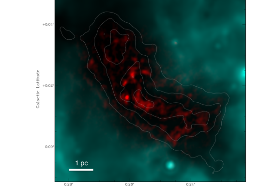
Figure 1: Combined infrared and millimetre image of G0.253+0.016  (24 $\mu$m  emission from the Spitzer Space Telescope  shown as cyan traces the heated dust from the Galaxy; 3 mm emission from ALMA shown as red traces the dust from the clump’s interior) overlaid with contours of the single-dish JCMT 450 $\mu$m  emission (contour levels are 30 to 90% of the peak, in steps of 20%). The scale bar marks a size scale of 1 pc. This cloud is so cold and dense it is seen as an extinction feature against the bright IR emission from the Galaxy. With the significant improvement in angular resolution and because ALMA sees through to the clump’s interior, we are now able to pinpoint the dust and gas within it and characterise its internal structure.

Our goal is to determine the location, mass, and kinematics of the small-scale fragments within G0.253+0.016. The new ALMA data reveal the internal structure and kinematics in this high-mass protocluster down to spatial scales of 0.07 pc (Fig. 1). As such, these data can be used to determine how the material is distributed within this protocluster.

2 ALMA observations

We imaged the 3 mm (90 GHz) dust continuum and molecular line emission across G0.253+0.016  using 25 antennas as part of ALMA’s Early Science Cycle 0. Because ALMA’s field of view at this wavelength is $\sim$ 1.2’ and the cloud is large on the sky (3’ $\times$ 1’), a 13-pointing mosaic was obtained to cover its full extent.

Using ALMA’s Band 3, the correlator was configured to use 4 spectral windows in dual polarization mode centred at 87.2, 89.1, 99.1 and 101.1 GHz each with 1875 MHz bandwidth and 488 kHz (1.4$-$1.7 km s^-1) channel spacing. With this setup we obtained the 3 mm dust continuum emission and also covered a number of excellent tracers of dense molecular and shocked gas, in particular: HCN, HCO⁺, C₂H, SiO, SO, H¹³CO⁺, H¹³CN, HN¹³C , HCC¹³CN, HNCO, H₂CS  CH₃SH, NH₂CHO, CH₃CHO, NH₂CN, and HC₅N  (for brevity in the text, we refer to the molecular transitions simply by the name of the molecule, e.g., HCN v=0 J=1–0  will be called ‘HCN’; see Table 1 for the quantum numbers of the transitions, frequency, critical densities, and excitation energies).

To build up the signal to noise and improve the $uv$-coverage, G0.253+0.016  was imaged on six different occasions over the period 29 July – 1 August 2012. We used the ALMA early science ‘extended configuration’; the projected baselines range from 13–455 m. All data reduction was performed using the CASA and Miriad software packages. Each individual dataset was independently calibrated (by our ALMA support scientist) before being merged together. We performed the cleaning and imaging to produce the final data products. Because the emission from adjacent 1.7 km s^-1  spectral channels are correlated, the final data cubes were resampled to have a velocity width of 3.4 km s^-1  per channel. The ALMA data have an angular resolution of $\sim$1.7″  ($\sim$0.07 pc), with a 1$\sigma$ continuum sensitivity of $\sim$ 25$\mu$Jy beam^-1 and line brightness sensitivity of 1.0 mJy beam^-1 per 3.4 km s^-1  channel.

3 Combination of the ALMA interferometric data with single dish data

Because the interferometric ALMA data are insensitive to emission on the largest angular scales ($>$ 1.2 ′), where possible we used single-dish data to fill in the missing zero-spacing information. Given that the emission from the clump is extended (3′$\times$1′) and the emission from the dust continuum and many of the molecular transitions on spatial scales $>$ 1.2′  significant, it was critical that the zero-spacing information was included to properly sample the $uv$-plane (e.g., Stanimirovic, 2002).

The combination of the ALMA data with the zero-spacing information was performed in the Fourier domain and was achieved using the corresponding single-dish data as a model during the CLEANing process. The inclusion of the single-dish data in this manner is superior to using alternatives task such as ‘feathering’ (see Ott, 2014 for details). For this technique to be applicable there must be an overlapping region of spatial frequencies between the two datasets. Fortunately, for both the continuum and line datasets, existing single-dish data provided the necessary coverage for inclusion with the ALMA data.

Ideally, the single dish data should have the same signal-to-noise as the interferometric data that they are being combined with. Although the signal-to-noise of the single dish data is lower than that of the ALMA data, it is high enough that the gain from recovering the zero-spacing information outweighs the increased noise that they may introduce.

To recover the zero-spacing information for the ALMA line cubes (HCN, HCO⁺, C₂H, SiO, HNCO), we used data from the MALT90 survey which were obtained using the Mopra 22 m telescope (Foster et al., 2011; Jackson et al., 2013; Rathborne et al., 2014a). To convert these data from T${}^{*}_{A}$  to the flux $F_{\nu}$ in Jy beam^-1, we used a scaling factor of 23 K/Jy beam^-1, calculated via the equation T${}^{*}_{A}$= 1.36 $\lambda^{2}$  $F_{\nu}$ /($\eta$ $\theta^{2}$), using a FWHM beam size, $\theta$, of 38″, wavelength, $\lambda$, of 3 mm, and a main beam efficiency, $\eta$, of 0.49 (Ladd et al., 2005).

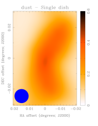
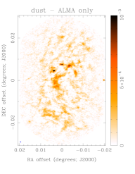
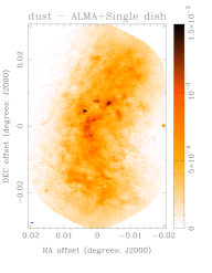
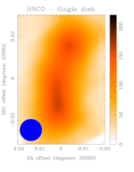
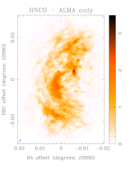
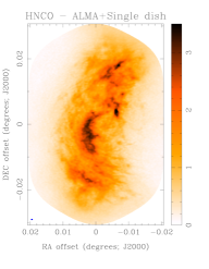
Figure 2: Images toward G0.253+0.016  showing both the significant improvement in angular resolution provided by ALMA and the recovery of the emission on the large spatial scales provided by the inclusion of the zero-spacing information. From left to right: Single dish, ALMA-only, and combined ALMA and single dish images. The upper row compares images of the 3 mm dust continuum emission (in units of mJy beam^-1), while the lower row compares images of the HNCO  integrated intensity emission (in units of mJy beam^-1 km s^-1). In all images the beam size is shown in the lower left corner. These (and all subsequent) images are shown in equatorial coordinates: the (0,0) offset position in R.A. and Dec is 17:46:09.59, $-$28:42:34.2 J2000.

For the continuum image, since we do not have a direct measurement of the emission at 3 mm on the larger angular scales, it was necessary to estimate the flux at 3 mm. To achieve this we scaled an image of the dust continuum emission at 500  $\mu$m  (Herschel, 33″  angular resolution) to what is expected at 3 mm assuming that the flux scales like $\nu^{(2+\beta)}$, where $\beta$ was assumed to be 1.2. Herschel data were used for this purpose as these data provide the most reliable recovery of the large scale emission. We choose to scale the 500  $\mu$m  Herschel image as it is the closest in wavelength to 3 mm, minimising the effect of the assumption of $\beta$ (see Rathborne et al., 2014b for more details). Figure 2 compares the single dish, ALMA-only, and combined (ALMA and single dish) images for both the continuum and the HNCO  integrated intensity. For the 3 mm dust continuum emission, the ALMA-only image recovers $\sim$18% of the total flux. The images clearly show the significant improvement in angular resolution provided by ALMA and the recovery of the emission on the large spatial scales provided by the inclusion of the zero-spacing information.

4 The small-scale structure within a cluster forming clump revealed

4.1 Continuum emission

Figure 1 shows a two colour image of G0.253+0.016  combining infrared images from the Spitzer Space Telescope  (24 $\mu$m, $\sim$6″  angular resolution, shown in cyan) with the new millimetre image from ALMA (3 mm, $\sim$1.7″  angular resolution, shown in red). Contours show single dish dust continuum emission (JCMT 450 $\mu$m , $\sim$ 7.5″  angular resolution). Identified as an infrared dark cloud (IRDC), G0.253+0.016  is clearly seen as a prominent extinction feature in mid-IR images. Because it is so cold, its thermal dust emission peaks at millimeter/sub-millimeter wavelengths. Moreover, since the 3 mm dust continuum emission is optically thin, internal structure is easily revealed by the ALMA images. While the overall morphology of the dust continuum emission revealed by ALMA matches well the mid-IR extinction and the large-scale dust continuum emission provided by the single dish image, the ALMA image shows significant structure on the small-scale. The emission is neither smooth nor evenly distributed across the clump; it is highly fragmented and there is a clear concentration of emission toward its centre. These small-scale fragments are presumably the cores from which stars may form.

Because the 3 mm continuum emission is optically thin , given standard assumptions about the dust emissivity, it can be used to determine the column density and, hence, mass of its small-scale fragments. Recent observations from Herschel of the 170–500  $\mu$m  dust continuum emission, show that the dust temperature (T_dust) within G0.253+0.016  decreases smoothly from 27 K on its outer edges to 19 K in its interior (Longmore et al., 2012). External to G0.253+0.016 , the dust temperatures are considerably higher, $>$35 K. Within the cloud and on the spatial scales probed by the Herschel data ($\sim$33″, $\sim$1 pc), no small volumes of heated dust are apparent. All of the millimetre emission detected by ALMA falls within the region for which T_dust  was measured to be $<$ 22 K. Thus, we assume that the temperature of the dust detected by ALMA ranges from 19–22 K and use a value of 20 $\pm$ 1 K for all calculations.

Assuming this dust temperature, a standard value of the gas to dust mass ratio of 100, a dust absorption coefficient ($\kappa_{3mm}$) of 0.27 cm² g^-1 (using $\kappa_{1.2mm}$ = 0.8 cm² g^-1, and $\kappa\propto\nu^{\beta}$ Chen et al., 2008; Ossenkopf & Henning, 1994,) and a $\beta$ of 1.2 $\pm$ 0.1 , the intensity of the 3 mm emission can be converted into the H₂  column density, N(H₂), by multiplying the measured fluxes by a single conversion factor of 1.9 $\times$10²³ ${\rm cm}^{-2}$ /mJy. We assume that T_dust  is constant across the cloud. For the small range of measured dust temperatures in G0.253+0.016, this approximation is well justified. Given these assumptions, the uncertainties for T_dust  and $\beta$ introduce an uncertainty of 10% for the column density, volume density, mass, and virial ratio.

The column densities across G0.253+0.016  measured from the ALMA-only image range from 0.5 - 82 $\times$ 10²² ${\rm cm}^{-2}$, with a mean value of 1.0 $\times$ 10²² ${\rm cm}^{-2}$. Since this image detects only the highest contrast peaks within the cloud and does not include the large-scale emission, we also determine the column density distribution using the combined (ALMA+SD) image which is more representative of the total column of material associated with G0.253+0.016. When including the emission on all spatial scales, we find that the mean column density is $\sim$ 8.6 $\times$ 10²² ${\rm cm}^{-2}$  and an order of magnitude higher compared to molecular clouds in the solar neighbourhood (see Rathborne et al., 2014b for a detailed discussion of the column density distribution across G0.253+0.016  and its comparison to solar neighbourhood clouds).

4.2 Molecular line emission: spectra, moment maps, channel maps, position velocity diagrams

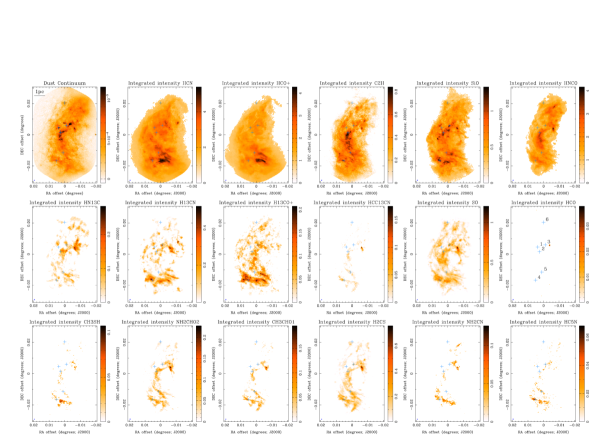
Figure 3: Dust continuum emission and molecular line integrated intensity images for G0.253+0.016. The molecular line images were generated by integrating the emission over the velocity range $-$10 km s^-1 $<$V_LSR $<$ 70 km s^-1  and clearly shows the differences in excitation conditions and chemistry across the clump. The continuum image is in units of mJy beam^-1, while the integrated intensity images are in units of mJy beam^-1 km s^-1. The angular resolution is shown in the lower left corner. All images in the top row have the large-scale emission included within them (i.e.  ALMA+SD). The images in the lower panels are ordered from left to right by increasing excitation energy. In all images the blue crosses mark the locations at which the spectra are plotted in Figure 5: the numbers are labelled on the HCO image.

The 3 mm (90 GHz) spectrum is rich in molecular lines that span a range in their excitation energies and critical densities (see Table 1). As such, these observations also provide data cubes from many molecular species and reveal a wealth of information about the gas kinematics and chemistry within G0.253+0.016. Figure 3 shows, along with the dust continuum image, the integrated intensity images for each of the detected molecular transitions. Clearly seen are the differences in the morphology of the emission from the various tracers, indicating that the chemistry and excitation conditions vary considerably within the clump.

To quantify the differences in the morphology of the integrated intensity for each molecular transition compared to the others and the dust continuum emission, we have determined the 2-D cross-correlation function for all combinations of image pairs. Figure 4 shows the derived correlation coefficients for each transition with respect to all others (the lower half of the figure shows the correlation coefficients via a colour scale, the upper half of the figure shows the derived values). For each particular tracer (labelled along the diagonal) the molecular transition for which it has the highest correlation coefficient can be found by searching for the darkest square either in the row to its left or in the column below (the corresponding values are mirrored in the upper portion of the figure).

We find that the morphology of the dust continuum emission is not highly correlated with any gas tracer, but is most correlated with the morphology of the emission from the molecules with high excitation energies (NH₂CHO  in particular). In addition, we find that the morphology of the emission from HCN  and HCO⁺  are highly correlated with each other and little else, that the shock tracers (SiO  and SO) are correlated with each other, and that the dense gas tracers with high excitation energies are well correlated with each other.

Figure 5 shows example spectra from the detected molecular transitions at several locations across the clump (spectra from a single pixel were extracted at the positions marked on Fig. 3 and listed in Table 2). The spectra clearly show the complexity of the emission and the differences in intensity and velocity detected from the various tracers. Molecular species with lower excitation temperatures (E_u/$k$ $\sim$4 K, e.g.,  HCN, HCO⁺, C₂H) show emission over a wider range in velocity ($\sim$ 10–15 km s^-1) compared to the isotolopogues (e.g.,  H¹³CN, H¹³CO⁺, HN¹³C , and HCC¹³CN; $\sim$3 –10 km s^-1) ) and those with higher excitation temperatures (E_u/$k$ $>$10 K, e.g.,  CH₃SH, NH₂CHO, CH₃CHO, H₂CS, NH₂CN, and HC₅N; $\sim$ 3 km s^-1). The shocked gas (traced by SiO  and SO) also shows emission over a wide range in velocity towards most locations in the clump ($\sim$ 3–20 km s^-1) .

For each molecular transition we characterise the emission via a moment analysis using the definitions of Sault et al. (1995). All moments were calculated over the velocity range $-$10 km s^-1 $<$V_LSR $<$ 70 km s^-1  (this range is delineated by dotted vertical lines on the spectra). The moment analysis allows us to characterise the emission at every point across the map and to easily compare the emission from the various molecular transitions to each other and to the dust continuum emission.

We compute the zeroth moment (M₀, or integrated intensity), the first moment (M₁, the intensity weighted velocity field), and the second moment (M₂, the intensity weighted velocity dispersion, $\sigma$). These are defined as

$$M_{0}=\int T_{A}^{*}(v)\,dv,\hskip 22.76219ptM_{1}=\frac{\int T_{A}^{*}(v)v\,dv}{\int T_{A}^{*}(v)\,dv},\hskip 22.76219ptM_{2}=\sqrt{\frac{\int T_{A}^{*}(v)(v-M_{1})^{2}\,dv}{\int T_{A}^{*}(v)\,dv}},$$

where T${}^{*}_{A}$$(v)$ is the measured brightness at a given velocity $v$. The peak intensity of the emission was also determined via a three-point quadratic fit to each spectrum (defined as moment $-$2; Sault et al., 1995 ). Note that C₂H  has well separated hyperfine components which will affect the first and second moment determinations (HCN also has hyperfine components, but their separation is less than the observed linewidth for HCN toward G0.253+0.016).

To include only the highest signal-to-noise emission in the moment analysis, the peak intensity, intensity weighted velocity field, and the intensity weighted velocity dispersion were only computed at positions across the clump where the emission was above an intensity threshold. For the emission from the molecular species that are the brightest and include the large-scale emission from the single dish data (i.e., HCN, HCO⁺, C₂H, SiO, and HNCO) we used a threshold in the integrated intensity of $>$ 20% of the peak. Since the noise level is different and the extended emission is included in these cases, this threshold was chosen so that the moments were calculated only when the emission was significantly detected above the noise. The choice of this threshold was visually checked (the region over which the moments were calculated are clearly outlined by the edges of the moment maps) to ensure that it was appropriate for the moment calculation. For the fainter lines with a lower signal to noise that do not include the large-scale emission, we used a threshold in the peak intensity of $>$ 3.8 mJy beam^-1  ($\sim$5$\sigma$).

At locations within the clump where the emission arises from well separated velocity features within the range $-$10 km s^-1 $<$V_LSR $<$ 70 km s^-1, the first moment (intensity weighted velocity field) will result in an intensity weighted average of their individual velocities. In addition, the second moment (intensity weighted velocity dispersion) will clearly be larger than the velocity dispersion of the individual velocity components. Thus, while this analysis may not describe well every individual velocity component, it does provide a method by which to easily characterise and compare the emission from the various tracers and the dust continuum across the clump.

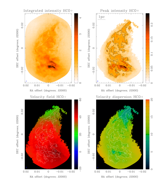
Figure 15: Moment maps for HCO⁺. Upper left: integrated intensity map (units of mJy beam^-1 km s^-1). Upper right: peak intensity map (units of mJy beam^-1). Lower left: intensity weighted velocity field (units of km s^-1). Lower right: intensity weighted dispersion (units of km s^-1). Overlaid on the latter three maps are contours of the peak intensity (levels are 30, 50, 70 and 90% of the peak). In all images the angular resolution is shown in the lower left corner.

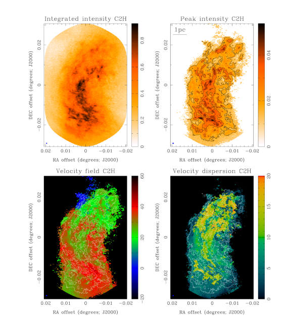
Figure 16: Moment maps for C₂H. Upper left: integrated intensity map (units of mJy beam^-1 km s^-1). Upper right: peak intensity map (units of mJy beam^-1). Lower left: intensity weighted velocity field (units of km s^-1). Lower right: intensity weighted dispersion (units of km s^-1). Overlaid on the latter three maps are contours of the peak intensity (levels are 30, 50, 70 and 90% of the peak). In all images the angular resolution is shown in the lower left corner.

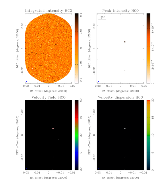
Figure 17: Moment maps for HCO. Upper left: integrated intensity map (units of mJy beam^-1 km s^-1). Upper right: peak intensity map (units of mJy beam^-1). Lower left: intensity weighted velocity field (units of km s^-1). Lower right: intensity weighted dispersion (units of km s^-1). Overlaid on the latter three maps are contours of the peak intensity (levels are 70% of the peak). In all images the angular resolution is shown in the lower left corner.

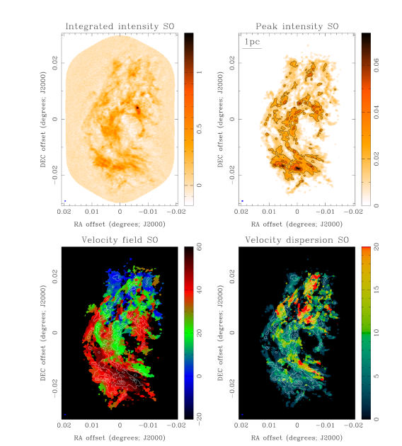
Figure 19: Moment maps for SO. Upper left: integrated intensity map (units of mJy beam^-1 km s^-1). Upper right: peak intensity map (units of mJy beam^-1). Lower left: intensity weighted velocity field (units of km s^-1). Lower right: intensity weighted dispersion (units of km s^-1). Overlaid on the latter three maps are contours of the peak intensity (levels are 30, 50, 70 and 90% of the peak). In all images the angular resolution is shown in the lower left corner.

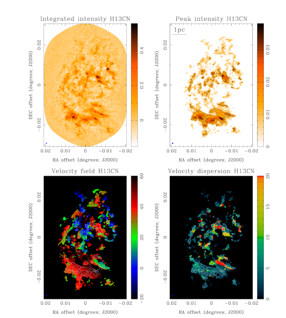
Figure 20: Moment maps for H¹³CN. Upper left: integrated intensity map (units of mJy beam^-1 km s^-1). Upper right: peak intensity map (units of mJy beam^-1). Lower left: intensity weighted velocity field (units of km s^-1). Lower right: intensity weighted dispersion (units of km s^-1). Overlaid on the latter three maps are contours of the peak intensity (levels are 30, 50, 70 and 90% of the peak). In all images the angular resolution is shown in the lower left corner.

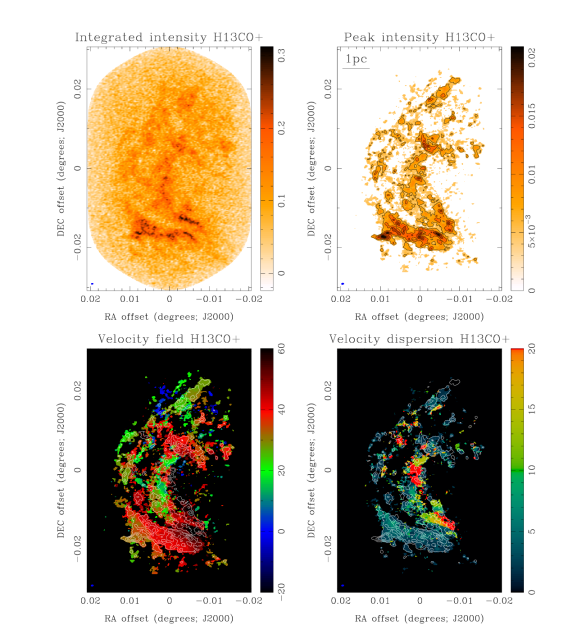
Figure 21: Moment maps for H¹³CO⁺. Upper left: integrated intensity map (units of mJy beam^-1 km s^-1). Upper right: peak intensity map (units of mJy beam^-1). Lower left: intensity weighted velocity field (units of km s^-1). Lower right: intensity weighted dispersion (units of km s^-1). Overlaid on the latter three maps are contours of the peak intensity (levels are 50, 70 and 90% of the peak). In all images the angular resolution is shown in the lower left corner.

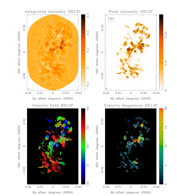
Figure 22: Moment maps for HN¹³C. Upper left: integrated intensity map (units of mJy beam^-1 km s^-1). Upper right: peak intensity map (units of mJy beam^-1). Lower left: intensity weighted velocity field (units of km s^-1). Lower right: intensity weighted dispersion (units of km s^-1). Overlaid on the latter three maps are contours of the peak intensity (levels are 30, 50, 70 and 90% of the peak). In all images the angular resolution is shown in the lower left corner.

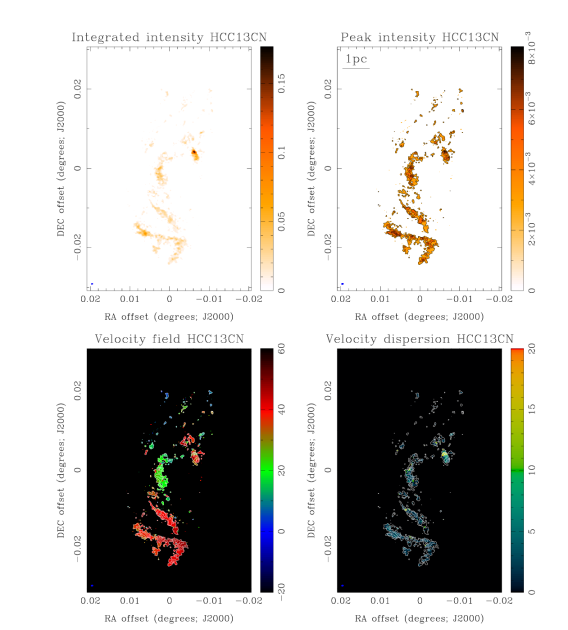
Figure 23: Moment maps for HCC¹³CN. Upper left: integrated intensity map (units of mJy beam^-1 km s^-1). Upper right: peak intensity map (units of mJy beam^-1). Lower left: intensity weighted velocity field (units of km s^-1). Lower right: intensity weighted dispersion (units of km s^-1). Overlaid on the latter three maps are contours of the peak intensity (levels are 30 and 70% of the peak). In all images the angular resolution is shown in the lower left corner.

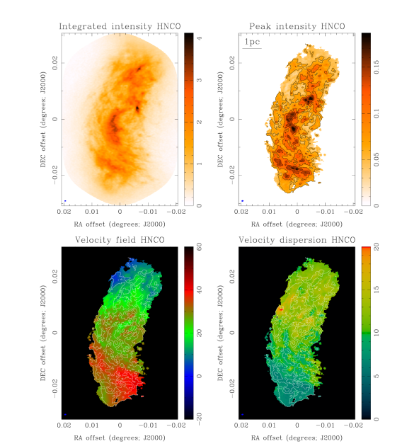
Figure 24: Moment maps for HNCO. Upper left: integrated intensity map (units of mJy beam^-1 km s^-1). Upper right: peak intensity map (units of mJy beam^-1). Lower left: intensity weighted velocity field (units of km s^-1). Lower right: intensity weighted dispersion (units of km s^-1). Overlaid on the latter three maps are contours of the peak intensity (levels are 30, 50, 70 and 90% of the peak). In all images the angular resolution is shown in the lower left corner.

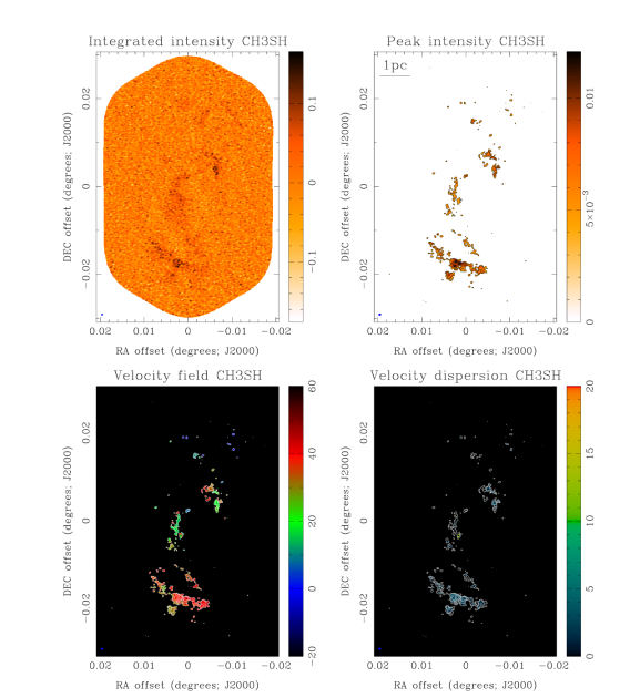
Figure 25: Moment maps for CH₃SH. Upper left: integrated intensity map (units of mJy beam^-1 km s^-1). Upper right: peak intensity map (units of mJy beam^-1). Lower left: intensity weighted velocity field (units of km s^-1). Lower right: intensity weighted dispersion (units of km s^-1). Overlaid on the latter three maps are contours of the peak intensity (levels are 30 and 70% of the peak). In all images the angular resolution is shown in the lower left corner.

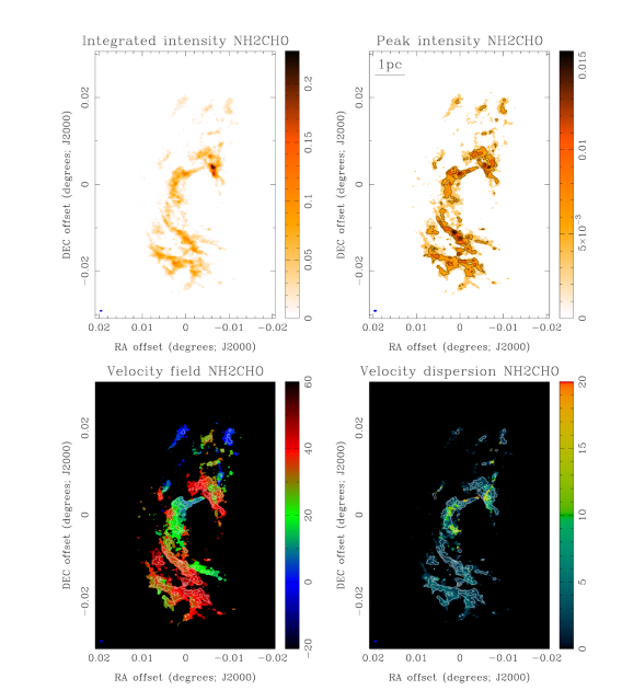
Figure 26: Moment maps for NH₂CHO. Upper left: integrated intensity map (units of mJy beam^-1 km s^-1). Upper right: peak intensity map (units of mJy beam^-1). Lower left: intensity weighted velocity field (units of km s^-1). Lower right: intensity weighted dispersion (units of km s^-1). Overlaid on the latter three maps are contours of the peak intensity (levels are 50, 70 and 90% of the peak). In all images the angular resolution is shown in the lower left corner.

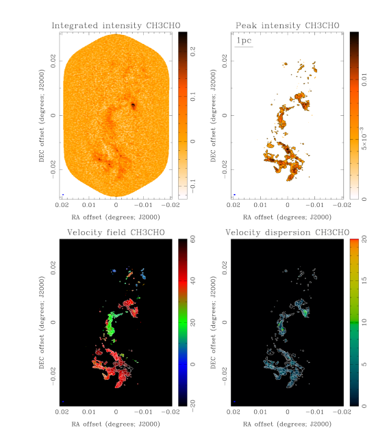
Figure 27: Moment maps for CH₃CHO. Upper left: integrated intensity map (units of mJy beam^-1 km s^-1). Upper right: peak intensity map (units of mJy beam^-1). Lower left: intensity weighted velocity field (units of km s^-1). Lower right: intensity weighted dispersion (units of km s^-1). Overlaid on the latter three maps are contours of the peak intensity (levels are 30, 50, 70 and 90% of the peak). In all images the angular resolution is shown in the lower left corner.

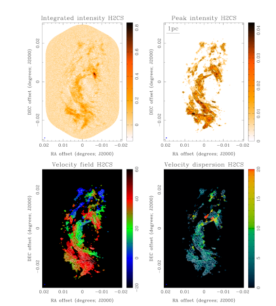
Figure 28: Moment maps for H₂CS. Upper left: integrated intensity map (units of mJy beam^-1 km s^-1). Upper right: peak intensity map (units of mJy beam^-1). Lower left: intensity weighted velocity field (units of km s^-1). Lower right: intensity weighted dispersion (units of km s^-1). Overlaid on the latter three maps are contours of the peak intensity (levels are 30, 50, 70 and 90% of the peak). In all images the angular resolution is shown in the lower left corner.

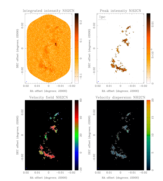
Figure 29: Moment maps for NH₂CN. Upper left: integrated intensity map (units of mJy beam^-1 km s^-1). Upper right: peak intensity map (units of mJy beam^-1). Lower left: intensity weighted velocity field (units of km s^-1). Lower right: intensity weighted dispersion (units of km s^-1). Overlaid on the latter three maps are contours of the peak intensity (levels are 30 and 70% of the peak). In all images the angular resolution is shown in the lower left corner.

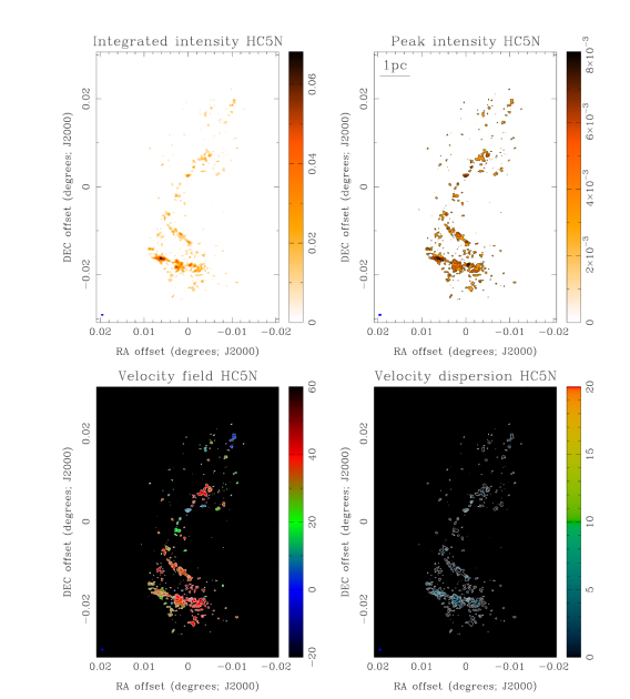
Figure 30: Moment maps for HC₅N. Upper left: integrated intensity map (units of mJy beam^-1 km s^-1). Upper right: peak intensity map (units of mJy beam^-1). Lower left: intensity weighted velocity field (units of km s^-1). Lower right: intensity weighted dispersion (units of km s^-1). Overlaid on the latter three maps are contours of the peak intensity (levels are 50, 70 and 90% of the peak). In all images the angular resolution is shown in the lower left corner.

Figure 6 shows the integrated intensity image (zeroth moment, M₀), peak intensity image, intensity weighted velocity field (first moment, M₁), and also the intensity weighted velocity dispersion (second moment, M₂) derived from the HCN  emission toward G0.253+0.016  (all other lines are included on-line in Figs. 15–30). Included on the latter three images are contours of the peak intensity: these highlight the small regions within the clump that are brightest and are included to aid in the comparison to the velocity field and dispersion images. All images showing the velocity field and dispersions use the same range of values for the colour coding (i.e., from $-$20 to 60 km s^-1  and from 0 to 20 km s^-1  respectively). This common colour coding for the different molecular transitions allows easy comparison and readily highlights differences between them.

The images of the velocity field clearly show the well known large-scale velocity gradient across the clump; most tracers of the dense gas show blue-shifted emission towards more positive declinations and red-shifted emission towards more negative declinations (i.e., SiO, SO, HNCO, and H₂CS). Some of the more complex molecules (NH₂CHO, CH₃CHO, and H₂CS) are also consistent with this trend. In contrast to the molecular transitions with lower excitation energies, the transitions from the more complex molecules also reveal emission toward the clump’s centre at $\sim$20 km s^-1  (coloured green in these images).

The obvious exception to these trends is seen in the emission from both HCN  and HCO⁺, which are clearly red-shifted across the whole clump and with respect to all other tracers. The trend that these optically thick gas tracers are systematically red-shifted with respect to the optically thin and hot gas tracers, indicates that G0.253+0.016  exhibits radial motions (either expanding or contracting, depending on the relative excitation temperatures of the inner and outer portions of the cloud, see Rathborne et al., 2014a for an in-depth discussion). The trend of red-shifted HCN  and HCO⁺  emission seen in the single-dish data remains in the interferometric data even when the single dish data are not included. Thus, radial motions are evident on all spatial scales.

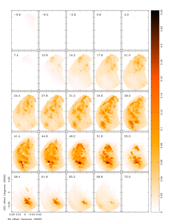
Figure 7: Channel maps for HCN. Each panel shows the emission (in units of mJy beam^-1) at the displayed velocity (in units of km s^-1). The angular resolution is shown in the lower left corner of each panel.

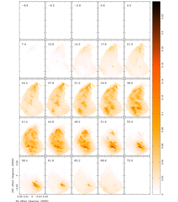
Figure 31: Channel maps for HCO⁺. Each panel shows the emission (in units of mJy beam^-1) at the displayed velocity (in units of km s^-1). The angular resolution is shown in the lower left corner of each panel.

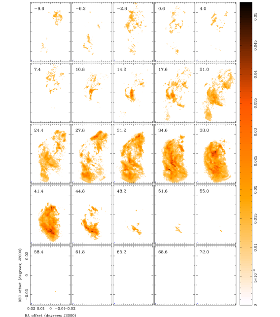
Figure 32: Channel maps for C₂H. Each panel shows the emission (in units of mJy beam^-1) at the displayed velocity (in units of km s^-1). The angular resolution is shown in the lower left corner of each panel.

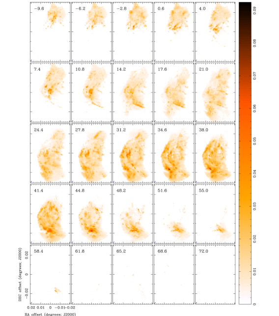
Figure 34: Channel maps for SiO. Each panel shows the emission (in units of mJy beam^-1) at the displayed velocity (in units of km s^-1). The angular resolution is shown in the lower left corner of each panel.

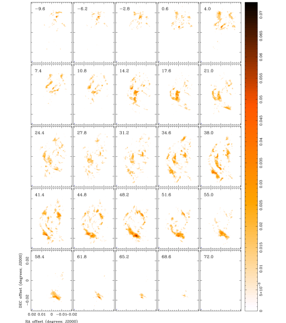
Figure 35: Channel maps for SO. Each panel shows the emission (in units of mJy beam^-1) at the displayed velocity (in units of km s^-1). The angular resolution is shown in the lower left corner of each panel.

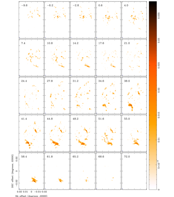
Figure 36: Channel maps for H¹³CN. Each panel shows the emission (in units of mJy beam^-1) at the displayed velocity (in units of km s^-1). The angular resolution is shown in the lower left corner of each panel.

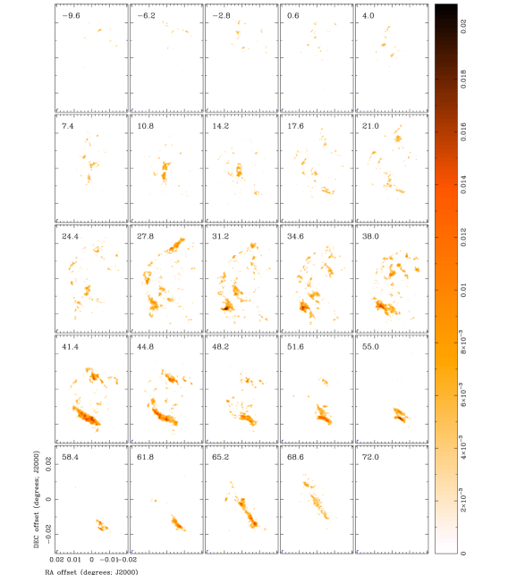
Figure 37: Channel maps for H¹³CO⁺. Each panel shows the emission (in units of mJy beam^-1) at the displayed velocity (in units of km s^-1). The angular resolution is shown in the lower left corner of each panel.

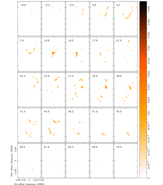
Figure 38: Channel maps for HN¹³C. Each panel shows the emission (in units of mJy beam^-1) at the displayed velocity (in units of km s^-1). The angular resolution is shown in the lower left corner of each panel.

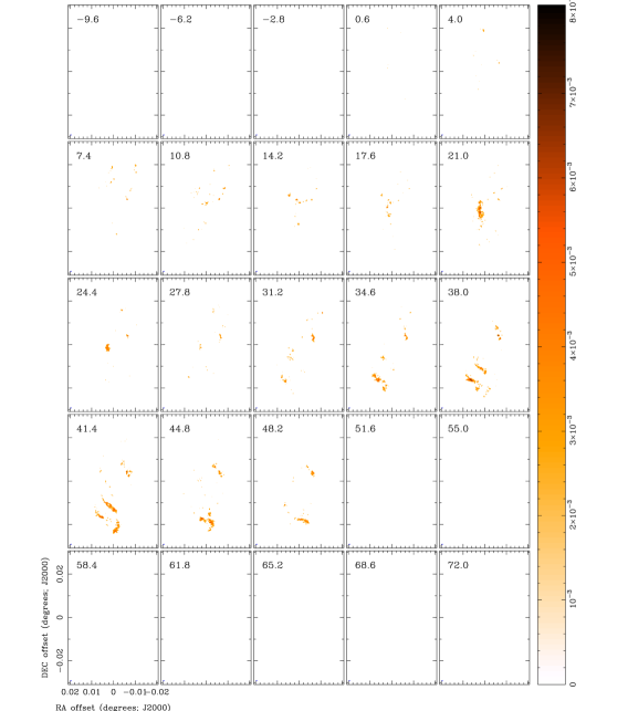
Figure 39: Channel maps for HCC¹³CN. Each panel shows the emission (in units of mJy beam^-1) at the displayed velocity (in units of km s^-1). The angular resolution is shown in the lower left corner of each panel.

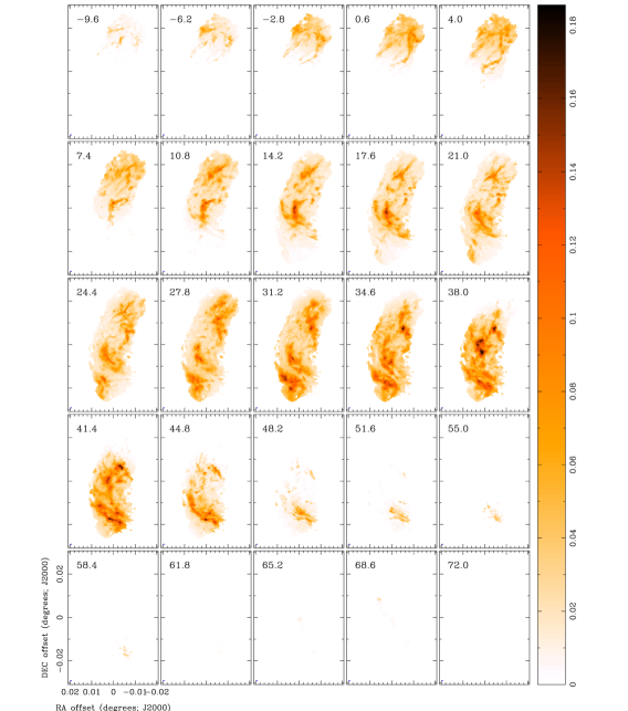
Figure 40: Channel maps for HNCO. Each panel shows the emission (in units of mJy beam^-1) at the displayed velocity (in units of km s^-1). The angular resolution is shown in the lower left corner of each panel.

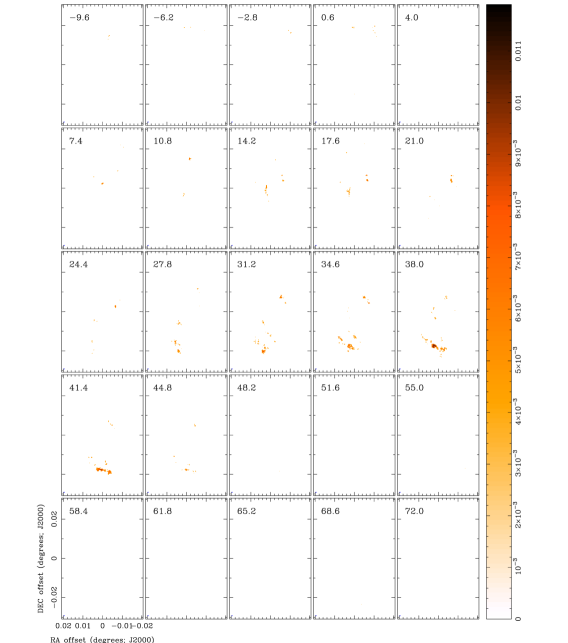
Figure 41: Channel maps for CH₃SH. Each panel shows the emission (in units of mJy beam^-1) at the displayed velocity (in units of km s^-1). The angular resolution is shown in the lower left corner of each panel.

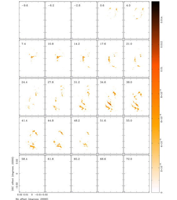
Figure 42: Channel maps for NH₂CHO. Each panel shows the emission (in units of mJy beam^-1) at the displayed velocity (in units of km s^-1). The angular resolution is shown in the lower left corner of each panel.

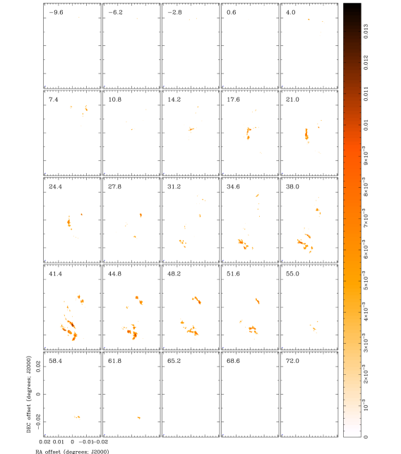
Figure 43: Channel maps for CH₃CHO. Each panel shows the emission (in units of mJy beam^-1) at the displayed velocity (in units of km s^-1). The angular resolution is shown in the lower left corner of each panel.

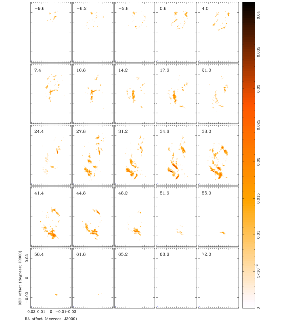
Figure 44: Channel maps for H₂CS. Each panel shows the emission (in units of mJy beam^-1) at the displayed velocity (in units of km s^-1). The angular resolution is shown in the lower left corner of each panel.

Figure 7 shows the channel maps for HCN  (all other channel maps are included on-line in Figs. 31–46). The panels show the emission from each spectral channel (the corresponding velocity is labelled in the top left corner of each panel) toward positions within the image where the emission was above the previously-defined intensity threshold. The channel maps also show well the clump’s large-scale velocity gradient. On the smaller scales, they reveal a complex network of emission features with a complicated velocity structure: there is emission on all spatial scales, the morphology of which ranges from small, compact regions to extended, filamentary structures. Toward many of the filamentary features we find homogeneous velocity fields, indicating that they are in fact physically coherent structures.

Surprisingly, we find filamentary features in both emission and in absorption. The absorption filaments are evident in the HCN  and HCO⁺  integrated intensity images and channel maps (i.e., Figs. 6, 15 and Figs. 7, 31 respectively). The most intriguing absorption filaments are those seen in HCO⁺ that extend for more than 20 km s^-1  in velocity. A detailed analysis of these features is discussed in Bally et al. (2014).

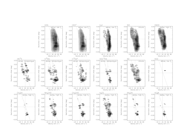
Figure 8: Position-velocity diagrams for each detected molecular transition. The dotted vertical line marks a velocity of 20 km s^-1, while the dotted horizontal line marks a positional offset of (0,0). The dotted diagonal line marks the velocity gradient that is evident across the clump. These lines are the same in all panels and are included to allow an easy comparison between panels. All position-velocity diagrams in the top row have the large-scale emission included within them (i.e.  ALMA+SD). The diagrams in the lower panels are ordered from left to right by increasing excitation energy. Each diagram is labelled with the ‘family’ to which the molecular transition belongs.

Position-velocity diagrams were also generated for each of the detected molecular transitions (Fig. 8). The major axis of the clump is defined along the 0-offset position in Right Ascension. The position-velocity diagrams were made by averaging the emission over the clump’s minor axis (i.e., in Right Ascension) and show the emission along the major axis (Declination) as a function of velocity. These diagrams also show the complexity in the emission and the systematic red-shift of the HCO⁺  and HCN  emission.

5 Statistical characterisation of the emission

Given the complexity of the clump’s structure and velocity field, we have employed several statistical methods in order to characterise the observed emission from the dust continuum and the various molecular transitions. Our goal is to answer the questions: How correlated is the emission from the various tracers with respect to one another? Which molecular line, if any, traces well the dust column density? Does turbulence set the observed structure? What is the structure of the gas; is it filamentary and hierarchically distributed or smooth and centrally condensed? Answers to these questions will reveal both the physical conditions within G0.253+0.016  and the mechanisms that are shaping its internal structure.

5.1 Molecular ‘families’ tell the same story

The combination of molecular transitions covered by these observations trace distinct chemical and physical conditions. For comparison, we group the molecules into four ‘families’: (1) those that have ‘low’ excitation energies E_u/$k$ $\sim$ 4 K (i.e., HCN, HCO⁺, C₂H), (2) those that are tracers of shocked gas (i.e., SiO  and SO), (3) the isotopologues (i.e., H¹³CN, H¹³CO⁺, HN¹³C , and HCC¹³CN), and (4) those that have ‘high’ excitation energies E_u/$k$ $\gtrsim$ 10 K (i.e., HNCO, CH₃SH, NH₂CHO, CH₃CHO, H₂CS, NH₂CN, and HC₅N).

Figures 9–11 compare the derived parameters from the moment analysis to the dust column density. These plots were generated by extracting the values from the moment maps and column density image at every pixel where there were non-zero values in both images . Because the number of plotted points within each panel is high, the data were binned so that a contour map of the distribution could be made. Contours show the overall distribution and location of the most common values (the contour levels are shown at 10 to 90% in steps of 10% of the peak number; the dotted contour outlines the 1% level). From top to bottom the rows show the normalised integrated intensities, normalised peak intensities, intensity weighted velocity field, and intensity weighted velocity dispersion as a function of dust column density. For ease of comparison, the molecular transitions are grouped according to the molecular ‘families’. Within each group the molecular transitions are ordered (from left to right) by increasing excitation energies (see Table 1 for the specific values).

Figure 9 shows the plots for HCN  and HCO⁺. For comparison, we show the same plots made including and excluding the large-scale emission (ALMA+SD and ALMA only; left and right respectively) to show the effect of its inclusion when calculating the intensity weighted moments. As expected, when including the large-scale emission, we find a clear correspondence between HCN  and HCO⁺  and the lower dust column density material (i.e., at column densities $<$ 5 $\times$ 10²² ${\rm cm}^{-2}$). These molecules clearly show an absence of blue-shifted emission, compared to most others (compare to Figs. 10 and 11). When the large-scale emission is included, the measured intensity weighted velocity dispersion is more centrally peaked (because the emission is widespread, with a broad line profile, the ‘intensity weighting’ will tend to result in a similar calculated value for the intensity weighted velocity despite the emission being detected over a broad range). Moreover, a clear trend is evident: the measured velocity dispersions decrease as the dust column density increases. This trend is not evident in the plots made with the ALMA-only data because, in this case, there is no emission from the molecular transitions at the same location as the low column density emission, which is required to see the trend.

The shock tracers (SiO and SO) show bright and widespread emission in both position and velocity across G0.253+0.016  (Fig. 10). Moreover, their measured velocity dispersions extend to $\sim$ 20 km s^-1, which is higher than most other tracers and expected since SiO and SO trace gas that is stirred up in regions of shocks. When including the large-scale emission, SiO  shows the opposite trend in its velocity dispersion compared to HCN  and HCO⁺: its velocity dispersion increases as the dust column density increases, consistent with increased shocks in the higher density material. For SO, while its typical measured dispersion is low ($\sim$ 2 km s^-1), there is a significant tail in this distribution up to dispersions of $\sim$ 20 km s^-1. In contrast to SiO, there is no clear trend for an increasing SO velocity dispersion with increased dust column density: SO shows low velocity dispersions regardless of the column density. The differences in the velocity dispersions measured for SiO and SO could be understood in terms of the differences in their excitation energies and critical densities : while SO has a higher excitation energy compared to SiO, it has a critical density which is an order of magnitude lower. Thus these species may in fact be tracing different material within the clump.

There are many filamentary features found within G0.253+0.016  that are detected in SiO and SO, that have high velocity dispersions, and large steps in velocity over small spatial regions (i.e., linear features seen in the moment maps in Figs. 18 and 19). Several of these are also evident in the channel maps of H¹³CN  (at LSR velocities of $\sim$ 10–17 km s^-1; see Figs. 34, 35, 36). They likely correspond to shock fronts within the clump: their details will be presented in a future paper.

The isotopologues and the molecular transitions with higher excitation energies (e.g., H¹³CN, H¹³CO⁺, HN¹³C , HCC¹³CN, HNCO, CH₃SH, NH₂CHO, CH₃CHO, H₂CS, NH₂CN, and HC₅N; Figs. 10 and 11), are detected over a much smaller range in dust column densities and are more sharply peaked at, or slightly above, the mean value of the dust column density ($\sim$ 8.6 $\times$10²²  ${\rm cm}^{-3}$, shown as the vertical dotted line) compared to the molecules with lower excitation energies. Their integrated intensity distribution appears bi-modal, indicating the presence of two distinct integrated intensity values. Their measured velocities span from 0 – 50 km s^-1; this velocity distribution is broader compared to that derived from HCN  and HCO⁺.

While the peak intensities for the isotopologues and the molecules with the higher excitation energies are smoothly distributed over a similar range in column densities to their integrated intensities, their velocity dispersion distributions are typically concentrated at low values of the velocity dispersion. With the exception of HNCO  which is far more abundant than these other molecules, we find that the emission predominantly arises from very narrow velocity features ($\sigma\lesssim$ 2 km s^-1). Such narrow velocity dispersions have also been observed toward G0.253+0.016  on small spatial scales from other molecular tracers (i.e. N₂H⁺ (3–2); Kauffmann et al., 2013). The tail in these distributions to considerably higher velocity dispersions (dotted contours), indicates positions within the clump where the moment analysis has overestimated the velocity dispersion due to multiple velocity components within the spectrum. This occurs in fewer than 1% of the spectra.

The narrow range in dust column density over which the higher excitation energy molecular transitions are detected can be understood in terms of their critical densities. These molecules are typically detected when the gas has either a high temperature (T_gas$>$100 K) or a high density (n $>$ n_crit), or both. Because these conditions are needed for both their formation and excitation, the presence of these molecules can be used to pinpoint gas with these physical conditions. These molecular transitions all have critical densities of $\sim 10^{5}-10^{7}$ ${\rm cm}^{-3}$  (see Table 1). Thus, while the gas temperature may be low toward the clump’s centre, the volume density may be very high. If the volume densities are sufficiently higher than their critical densities, the molecules may be excited regardless of the gas temperature.

We see a clear trend that molecules with higher excitation energies and critical densities peak toward the centre of the clump (compared to those with lower excitation energies and critical densities). The position-velocity diagrams also reveal that the molecular transitions with higher excitation energies and critical densities peak toward the centre of the cloud in both position and velocity (declination offset of $\sim$ 0, and velocity of $\sim$ 20 km s^-1; e.g.  CH₃CHO  and NH₂CN  in Fig. 8). These trends are exactly what is expected for a clump with a denser interior.

5.2 Which molecules can be used to assess the dynamical state of the cores?

While the molecular transitions detected by these observations all probe dense gas, they span a range in their critical densities and excitation energies, trace distinct chemical conditions, and often suffer from high optical depths. As such, they may often trace different material within G0.253+0.016  and may not necessarily correlate well with the optically thin dust continuum emission.

One of our key goals is to identify star-forming dust cores within the clump, to measure their sizes, masses, and virial state. Determining these properties will allow us to ascertain the potential of G0.253+0.016  to form a cluster and the distribution of masses for its cores. In order to identify bound star-forming cores, we need to reliably associate molecular line emission with each dust continuum core in order derive their velocity dispersions. Ideally, we need to identify a molecular transition that is optically thin and is bright enough to be detected in most cores.

Given the limited velocity resolution of our data, a detailed analysis of the cores’ virial states are challenging with the current data. However, we can gauge, overall, which molecular transitions correlate with the dust emission. We find that emission from the molecular transitions with higher excitation energies typically provide a better morphological match to the dust column density compared to the transitions with lower excitation energies, the isotopologues, or the shock tracers (compare the morphology of the dust emission to NH₂CHO, CH₃CHO, HNCO  and H₂CS  in Fig. 3 and also their 2-D correlation coefficients shown in Figure 4). Moreover, since their velocity dispersions are typically narrow ($\sim$ 2 km s^-1), these molecules may in fact be tracing individual high column density cores within the clump with very narrow velocity dispersions.

5.3 Is the gas structure set by turbulence?

Supersonic turbulence is an important mechanism by which overdensities within molecular clouds may be generated (Vázquez-Semadeni, 1994; Padoan et al., 1997). As such, understanding the degree to which turbulence sets the initial structure within molecular clouds is an important part of understanding core and, ultimately, star formation. Recent work using the ALMA dust continuum emission presented here shows that the log-normal shape, dispersion, and mean of its column density probability distribution function (N-PDF) very closely matches the predictions of theoretical models of supersonic turbulence in gas given the high-pressure environment in which G0.253+0.016  is immersed (Rathborne et al., 2014b).

These results also show that while, overall, the N- PDF shows a log-normal distribution, there is a small deviation from log-normal at the highest column densities, which indicates self-gravitating gas. This small deviation is coincident with the location of a known water maser (Lis & Carlstrom, 1994) and, thus, pinpoints where star formation is beginning in the cloud. Assuming a dust temperature of 20 K, this small core (radius of 0.04 pc) has a mass of $\sim$72 M_⊙  and virial ratio, $\alpha_{\rm vir}$, of $\lesssim$ 1 (this is an upper limit since the associated molecular line emission is unresolved in velocity, $\sigma<$ 1.4 km s^-1; see Rathborne et al., 2014b for details). Since $\alpha_{\rm vir}$ is close to unity, this core is gravitationally bound and unstable to collapse.

The fact that the N-PDF for G0.253+0.016  matches well predictions from turbulent theory suggests that our current understanding of molecular cloud structure derived from the solar neighbourhood also holds in high-pressure environments (Rathborne et al., 2014b). This has important implications for understanding the initial gas structure for star formation in a range of different environments across the Universe (Kruijssen & Longmore, 2013).

To further determine the extent to which turbulence shapes the observed gas structure within G0.253+0.016, we have calculated the fractal dimension and the turbulent power spectrum. These statistical methods are commonly used to describe the structure of molecular clouds in both simulations and observations.

5.3.1 Fractal structure on small spatial scales

An important characteristic of a protocluster clump, and one that is easily revealed by these data, is the distribution of its material on small spatial scales. If G0.253+0.016  represents a clump that will give rise to a high-mass cluster, then the distribution of the material within it before star formation has commenced can provide important constraints for theories that describe cluster formation. As discussed previously, there have been a wide range of theoretical and numerical studies showing that the formation of high-mass stellar clusters should proceed hierarchically, but thus far the degree of hierarchal structure within high-mass protoclusters has not been estimated.

The fractal dimension (D_f) can be used to characterise the structure within a molecular cloud. It is a simple tool that determines the degree to which the emission is smooth and centrally condensed or structured and hierarchical. Since observations of dust or molecular line emission reveal only the 2 dimensional projection of a 3 dimensional structure, care needs to be taken to accurately convert the measured projected fractal dimension (D_p) to the real three-dimensional fractal dimension (D_f). This conversion is often assumed to be D_f = D_p + 1 (Beech, 1992); however, using simulations of cloud structure, Sánchez et al. (2005) derive an empirical relation to convert between D_f and D_p (see their figure 8). Rather than a single conversion factor of unity for all values of D_p, their simulations suggest that D_f may actually increase linearly as D_p decreases. Previous observations derive projected fractal dimensions D${}_{p}\sim$ 1.35 (see Federrath et al., 2009 and references therein) leading to a quoted D_f for molecular clouds of $\sim$ 2.3 (Elmegreen, 1997).

To calculate the projected fractal dimension (D_p) for G0.253+0.016, we employ the perimeter-area method (Mandelbrot, 1977) which is often used to measure the fractal dimension of interstellar gas clouds (e.g., Falgarone et al., 1991; Federrath et al., 2009; Sánchez et al., 2005). Structures were defined as connected regions within a contour at a given intensity level. The area (A) was calculated as the sum of the number of pixels within the contour, the perimeter (P) was calculated as the number of pixels externally adjacent to the contour level. By varying the contour levels from the image minimum to its maximum, values for P and A were determined on many spatial scales. With a power-law fit of the form P $\propto$ A ${}^{D_{p}/2}$, we can determine the perimeter-area fractal dimension D_p. A smooth structure will have D_p = 1, while a very convoluted structure will have D_p = 2 (Federrath et al., 2009).

Figure 12 shows the perimeter-area plots measured from contours of the dust and line integrated intensity emission. For this analysis we use, where possible, the data that includes the large-scale emission. Since this analysis is based on contours within an image, the effect of including the large-scale emission simply increases the number of contours to lower levels of the intensity which translates to an increase in the number of points plotted at large perimeters and areas. Their inclusion has little effect on the derived slope.

In all panels the solid lines show two extreme values for D_p (1 for smooth, centrally condensed emission, 2 for a highly fractal cloud). The dotted lines show linear fits to the data points: the derived values for D_p range from 1.4–1.7, depending on the molecular tracer. For the dust continuum that includes the large-scale emission, we find a D_p of 1.6 (plotted in the top left panel, marked as ALMA+SD). For comparison we also calculate the fractal dimension derived from only the large-scale dust continuum emission (in the same panel marked as SD), and find D_p to be $\sim$1.2, consistent with its smooth distribution.

Since the fractal dimension is best indicated by emission that is optically thin, i.e., from the dust emission and the molecular transitions with higher excitation energies, we select the derived D_p from these molecules to characterise the emission from within G0.253+0.016  (i.e., D_p $\sim$ 1.6). Using the empirical conversion from the two-dimensional fractal dimension D_p to the three-dimensional fractal dimension D_f from Sánchez et al. (2005), we find that D_f $\sim$ 1.8 for G0.253+0.016. Simulations of compressively driven turbulence in the ISM (Federrath et al., 2009) with Mach numbers, $\mathcal{M}$, of $\sim$ 5.5, reveal typical values for D_f of 2.3–2.6 (which correspond to D_p $\sim$ 1.3–1.5 using the empirical relation derived by Sánchez et al., 2005) . Since $\mathcal{M}$  is $\sim$ 30 for G0.253+0.016, it has a much higher level of turbulence compared to most other molecular clouds. Given this higher level of turbulence, it may be expected that the sonic length may be lower and the degree of fragmentation might be higher in G0.253+0.016  (i.e. a higher D_p, and thus, lower D_f for higher $\mathcal{M}$). While detailed simulations are necessary to determine the effect of $\mathcal{M}$  on the fractal dimension, our results are consistent with a marginally higher value for D_p for G0.253+0.016  when compared to typical molecular clouds. This analysis suggests that the clump is highly fragmented on small spatial scales and its structure consistent with that produced by compressively driven turbulence.

5.3.2 Turbulent power spectrum

The power spectrum provides a measure of how turbulence is propagated within a molecular cloud and it identifies the preferential spatial scale, if any, at which the structure changes. On large scales a break in the power spectrum indicates the spatial scale at which turbulent energy is injected, on the small scales it can indicate the spatial scales at which either turbulence is dissipated or injected . Measuring the small-scale break point of the power spectrum can therefore reveal the spatial scale at which gravity overcomes the turbulent pressure or the spatial scale at which energy may be injected (i.e. from protostellar outflows) .

We use the dust continuum image and several of the integrated intensity images to compute the power spectra. Because the turbulent power spectrum is a statistical measure of the energy on various spatial scales, it is important that the emission is well detected and well sampled across the clump. As such, we perform this analysis using HCN, HCO⁺, HNCO, and SiO  because their data include the zero-spacing information and the emission is detected with high signal-to-noise ratios at all spatial scales across G0.253+0.016.

Figure 13 shows the annular averages of each of the power spectra, P(k), as a function of the spatial frequency, k. The power spectra were generated using a Fast Fourier Transform of the images. In all panels the dotted vertical line marks the spatial frequency corresponding to the angular resolution of the data: the power spectra at spatial frequencies greater than this are not well sampled by these data.

In cases where the power spectrum is close to a power law (i.e., for HCN, HCO⁺, HNCO, and SiO  emission) we fit it with a single power law to derive $\alpha$ where, P(k) $\propto$ k^-α. In these cases, we find that $\alpha\sim$ 3. A power-law slope of 3 is predicted for a line intensity power spectrum of an optically thick medium (Lazarian & Pogosyan, 2004; Burkhart et al., 2013). Thus, the derived power spectrum slope of $\sim$ 3 for these molecular transitions are consistent with them being optically thick toward G0.253+0.016.

In contrast, for the dust continuum emission which is optically thin, the power spectrum shows a clear break. While this break occurs at large spatial frequencies (i.e. small spatial scales), it is lies above the spatial frequencies corresponding to the angular resolution of these data (marked with the vertical dotted line). For this power spectrum we fit two distinct power laws and derive their indicies and the break point. For small values of k (i.e., large spatial scales) the derived power-law index is $\alpha\sim$ 2.9 compared to $\alpha\sim$ 7.5 for large values of k (i.e., small spatial scales). Values for $\alpha$ of $\sim$ 2.8 are observed toward other star-forming regions such as Perseus, Taurus and Rosetta (Padoan et al., 2004).

The trend of a steeper spectrum on smaller spatial scales implies that the higher column density material is concentrated on smaller spatial scales, while the lower column density material is distributed on larger spatial scales. This is consistent with the distribution of the emission in the dust continuum image. Since the effect of gravity on small scales will cause a steepening of the power-law slope at large spatial frequencies , the spatial scale at which gravity may dominate can be determined from the break point in the power spectrum. From the dust continuum emission power spectrum, we find that the break occurs at spatial frequencies corresponding to size scales of $\sim$0.09 pc. This size scale is comparable to the size of the small region of self-gravitating gas that was identified as the deviation at high column densities via the N-PDF (Rathborne et al., 2014b). As such, this lends support to the idea that gravity has overcome the internal pressure on these small spatial scales.

For cores within molecular clouds to collapse into stars, they need to be sufficiently dense that their self-gravity overcomes the thermal pressure . The Jeans length, defined as the minimum length scale for gravitational fragmentation to occur, was determined for G0.253+0.016  using the relation

$$\lambda_{J}=0.4\,pc\left(\frac{c_{s}}{0.2\,kms^{-1}}\right)\left(\frac{n(H_{2})}{10^{3}\,cm^{-3}}\right)^{-0.5}$$ (1)

where $c_{s}$ is the sound speed and n(H₂) the volume density. While the measured dust temperature toward G0.253+0.016  is $\sim$ 20 K (Longmore et al., 2012), recent observations indicate that the gas temperature is considerably higher, $\sim$ 65 K (Ao et al., 2013), leading to the speculation that the gas may be heated by the dissipation of turbulent energy and/or cosmic rays rather than by photon heating. These observations are supported by SPH modelling of the dust and gas temperature distribution in G0.253+0.016  which suggest that the gas and dust temperatures are not coupled and that the high interstellar radiation field (ISRF) and cosmic ray ionisation rate (CRIR) in the CMZ are responsible for the discrepant dust and gas temperatures (Clark et al., 2013).

Assuming a global gas temperature for G0.253+0.016  of 65 K (Ao et al., 2013) the corresponding gas sound speed, $c_{s}$, is 0.5 km s^-1. Using an average volume density for this material of $\sim$ 10⁵ ${\rm cm}^{-3}$, we derive $\lambda_{J}$ to be 0.10 pc. This value is comparable to the size scale derived from the break point in the power spectrum of the dust continuum emission and of the size of the self-gravitating core identified via the N-PDF. Extrapolating the global size-linewidth relation in Figure 14 (top right panel) to smaller scales, suggests that the line-widths are subsonic on spatial scales of $\sim$0.1 pc (the sonic length is $\sim$ 0.2 pc). As such, since the sonic length exceeds the derived break point in the power spectrum, the thermal Jeans length is indeed the relevant quantity for describing the minimum size scale for gravitational fragmentation . An absence of a similar break in the power spectra derived from the molecular line emission is consistent with the transitions being optically thick and the dust continuum optically thin. Thus, the small, high-column density features detected in the optically thin dust continuum emission may have formed because gravity was able to overcome the thermal pressure on these small scales.

6 Implications for the formation of young massive clusters

Observations show that YMCs like the Arches are very centrally condensed, with stellar masses of $>$10⁴ M_⊙  within their central 0.5 pc (Portegies Zwart et al., 2010). If G0.253+0.016  is the molecular cloud progenitor to a cluster like the Arches, then its internal structure can reveal the initial conditions for the formation of such high-mass clusters and whether or not the central concentration of stellar densities arises directly from the initial gas structure.

To determine its internal structure, we have calculated the mass and volume density profiles of G0.253+0.016  as a function of radius (left panels of Fig. 14). We define each region over which to calculate the mass and volume density using contours of column density; they were calculated on many spatial scales by varying the contour levels from the lowest to the highest values. An ‘effective radius’ was determined for each region by summing the number of pixels contained within that contour level and assuming that this area, A, forms a circle such that $R_{eff}=\sqrt{A/\pi}$. The mass within each region was then calculated by summing the column density, the volume density is calculated by dividing the mass by the volume of a sphere with a radius of $R_{eff}$ (left panels of Fig. 14).

Using the detected emission from the various molecular species, we have also calculated the average velocity dispersion and virial ratio as a function of radius (right panels of Fig. 14). The virial ratio is $\alpha_{\rm vir}$, defined as $\alpha_{\rm vir}=5\sigma^{2}R/GM$, where $\sigma$ is the measured velocity dispersion, $R$ the radius, $G$ the gravitational constant, and $M$ the mass. For these calculations the ‘effective radius’ was determined from the total number of pixels within the integrated intensity image for each of the molecular transitions. Within these regions the total mass, $M$, was determined from the dust column density summed over the same region, while $\sigma$ was determined by averaging the intensity weighted velocity dispersions.

The ALMA observations of the gas structure within G0.253+0.016  show that the material is distributed in a complex, filamentary network of structures that are highly fragmented. Its volume density profile (lower left panel of Fig. 14) shows that the average volume density increases with smaller radii, suggesting that the material is more concentrated toward the clump’s centre. We find that the volume density profile follows very well a power law for radii $<$ 2 pc with an index of $\sim-$1.2. In contrast to what is expected for a Bonner-Ebert sphere and Plummer models that are often used to describe the volume density profiles within starless cores and globular clusters, the volume density profile for G0.253+0.016  shows no flattening at small radii.

While the total mass of G0.253+0.016  is $\sim$ 10⁵ M_⊙, its mass profile shows that the majority of the mass originates from the low column density material in its outer edges, at large radii (upper left panel of Fig. 14). We find that the average velocity dispersion decreases on small spatial scales (upper panel of Fig. 14), similar to the results of Kauffmann et al. (2013). Moreover, we find that the derived virial ratios are $>$ 1 for the molecular emission that is widespread (i.e. have large effective radii) but $<$ 1 for the molecular species that are detected only over smaller regions (lower panel of Fig. 14). This trend of decreasing virial ratios as the radius decreases, implies that G0.253+0.016  is unbound at large radii, but bound at smaller radii. Thus, its outer envelope of lower density material may be unbound and expanding, while the inner denser region is bound and, in the absence of other supporting mechanisms, may be collapsing.

The notion that the G0.253+0.016  may have a dense and collapsing interior with a low-density surface that is expanding was posed recently by Bally et al. (2014) when discussing the nature and origin of the HCO⁺  absorption filaments seen toward G0.253+0.016. This idea is supported by the observations of the large scale gas motions which show systematically red-shifted optically thick emission compared to the optically thin and hot gas tracers (Rathborne et al., 2014a). In this scenario, the exterior layers of the cloud have a lower excitation temperature compared to the inner layers of the cloud, because the emission is sub-thermally excited (n$<<$n_crit). The expanding outer regions, coupled with a collapsing inner region, is consistent with the scenario in which G0.253+0.016  was formed recently as a result of a pericentre passage close to Sgr A^∗ (Longmore et al., 2013; Kruijssen et al., 2014a)

While a gravitationally bound and collapsing clump is consistent with what is expected in the very early stage of mass assembly within a protocluster, we find that there is no large concentration of mass in the centre of G0.253+0.016. Indeed, its total mass within a radius of 0.5 pc is only $\sim$ 6 $\times$ 10³ M_⊙: this is insufficient to form an Arches-like cluster by more than 2 orders of magnitude. Indeed, recent work characterising the structure within other high-mass, dense clumps in the CMZ show that the lack of a strongly peaked central mass distribution may be a general trend within these YMC-progenitor clouds (Walker et al., submitted). Thus, if G0.253+0.016  is destined to form a high-mass ($>$10⁴ M_⊙) cluster, then the structure of the resulting cluster must evolve from this initial dispersed, hierarchical structure to a smooth, centrally condensed configuration via a dynamical process (e.g. Allison et al., 2010; Moeckel & Bate, 2010; Kruijssen et al., 2012; Parker & Dale, 2013; Parker et al., 2014) . As such, any model for cluster formation that posits that stars form directly from an initially smooth, central concentration of gas with a mass similar to that of the final stellar cluster (e.g. Lada et al., 1984; Geyer & Burkert, 2001; Boily & Kroupa, 2003; Goodwin & Bastian, 2006; Baumgardt & Kroupa, 2007) , is ruled out by these observations.

7 Conclusions

Using observations from the new ALMA telescope we have conducted a statistical analysis of the small-scale structure and velocity within the high-mass protocluster clump G0.253+0.016. Its 3 mm dust continuum and molecular line emission reveal a complex network of emission features that have a complicated velocity structure. Filamentary structures, that are coherent in velocity, are seen in both emission and absorption.

Widespread emission is detected from 17 different molecular transitions that probe a range in distinct physical and chemical conditions. Comparing their intensity, velocity dispersion, and velocity fields, we find that the molecular ‘families’ trace the same type of material with the clump: transitions that are optically thick have broad velocity dispersions and trace material on the large scales, while transitions that are optically thin have narrow velocity dispersions and trace the densest material in the clump’s centre. Indeed, the dust column density is best traced by molecules with higher excitation energies and critical densities, consistent with a clump that has a denser interior.

The emission is found to be highly fragmented (D${}_{f}\sim$ 1.8), consistent with structure that is produced by compressively driven turbulence. We find a clear break in the turbulent power spectra derived from the optically thin dust continuum emission at a spatial scale of $\sim$ 0.1 pc. This size scale is comparable to the Jeans length corresponding to the observed gas density and temperature, and also to the size of the small core of self-gravitating gas that was identified from the N-PDF. Thus, these structures might correspond to the spatial scale at which gravity has overcome the turbulent pressure.

We speculate that G0.253+0.016  is on the verge of forming a cluster from hierarchical, filamentary structures that arise from a highly turbulent medium. Because the initial gas structure is fractal and hierarchical, its structure is quite different from the smooth, compact, very centrally condensed structure observed in high-mass clusters. Consequently, these observations rule out models of cluster formation that begin with such gas distributions. The implication is that if stars within YMCs form from hierarchical gas structures such as these observed in G0.253+0.016, then their distribution must change to a more centrally condensed configuration over a dynamical time scale. Thus, any theoretical study that aims to accurately characterise and understand the early phases of cluster formation ought to begin with an initial gas structure that is hierarchical rather than one that is smooth and centrally concentrated.

Table 1: Summary of the molecular transitions detected toward G0.253+0.016^a.

	Molecular transitionb	Frequency	Eu/$k$	ncrit	Name
		(GHz)	(K)	(${\rm cm}^{-3}$)
Dense, ‘low’ Eu/$k$:
	HCN v=0 J=1–0	88.632	4.25	1$\times 10^{6}$	Hydrogen Cyanide
	HCO+ v=0 J=1–0	89.189	4.28	1$\times 10^{5}$	Formylium
	HCO 1(0,1)–0(0,0), J=3/2-1/2, F= 2- 1	86.671	4.18	$\sim$ 3$\times 10^{5}$	Formyl Radical
	C2H v = 0 N=1–0, J=3/2-1/2, F= 2- 1	87.317	4.19	4$\times 10^{5}$	Ethynyl
Shocks:
	SiO v = 0 J=2–1	86.847	6.25	2$\times 10^{6}$	Silicon Monoxide
	SO v = 0 3(2)–2(1)	99.300	9.23	3$\times 10^{5}$	Sulfur Monoxide
Isotolopologues:
	H13CN v = 0 J=1–0	86.340	4.14	9$\times 10^{5}$	Hydrogen Cyanide, isotopologue
	H13CO+ J=1–0	86.754	4.16	1$\times 10^{5}$	Formylium, isotopologue
	HN13C J=1–0	87.091	4.18	1$\times 10^{5}$	Hydrogen Isocyanide, isotopologue
	HCC13CN v = 0 J=11–10	99.661	28.70	$\sim$ 8$\times 10^{6}$	Cyanoacetylene, isotopologue
Dense, ‘high’ Eu/$k$:
	HNCO v=0 4(0,4)–3(0,3)	87.925	10.55	4$\times 10^{6}$	Isocyanic Acid
	CH3SH v = 0 4(0)+-3(0)+A	101.139	12.14	$\sim$ 9$\times 10^{5}$	Methyl Mercaptan
	NH2CHO 4(1,3)–3(1,2)	87.849	13.52	$\sim$ 4$\times 10^{6}$	Formamide
	CH3CHO v=0 5(1,4)–4(1,3) E	98.863	16.59	$\sim$ 3$\times 10^{6}$	Acetaldehyde
	H2CS 3(1,3)–2(1,2)	101.478	22.91	2$\times 10^{5}$	Thioformaldehyde
	NH2CN 5(1,4)–4(1,3), v=0	100.629	28.99	$\sim$ 9$\times 10^{6}$	Cyanamide
	HC5N v = 0 J=33–32	87.864	71.69	$\sim$ 9$\times 10^{6}$	Cyanobutadiyne

Table 2: Summary of the positions across G0.253+0.016  from which spectra are displayed in Figure 5.

Position					Comment
	R.A.	Dec.	Offset R.A.	Offset Dec.
	(deg)	(deg)	(deg)	(deg)
1	17:46:10.628	–28.:42:17.75	0.004	0.004	Peak in the dust column density
2	17:46:10.308	–28.:42:28.60	0.003	0.001	Centre of the clump
3	17:46:09.297	–28.:42:12.50	–0.001	0.006	Position showing multiple velocity components
4	17:46:11.000	–28.:43:34.05	0.005	–0.017	Lower part of the clump, where most molecules are detected
5	17:46:09.883	–28.:43:15.50	0.001	–0.012	Lower part of the clump, where the linewidths from the molecules are very different
6	17:46:09.590	–28.:41:20.70	0.000	0.020	Upper part of the clump, dust continuum peak

Figure 4: 2-D cross-correlation coefficients for each tracer with respect to all others (the lower half of the figure shows the correlation coefficients via a colour scale, the upper half of the figure shows the derived values). For each particular tracer (labelled along the diagonal) the molecular transition for which it has the highest correlation coefficient can be found by searching for the darkest square either in the row to its left or in the column below (the corresponding values are mirrored in the upper portion of the figure). Overall, the dust continuum emission is not highly correlated with any gas tracer, but is most correlated with the morphology of the emission from the molecules with high excitation energies (NH₂CHO  in particular). As expected, the tracers within each molecular ‘family’ are most correlated with each other.

Figure 5: Example spectra selected from 6 positions across G0.253+0.016  (see Figure 3 and Table 2 for more details). The molecular transitions are ordered, from top to bottom, in increasing excitation energies. The dotted lines delineate the range in velocity over which the moments were computed ($-$10 km s^-1 $<$V_LSR $<$ 70 km s^-1). Note that C₂H  has a second hyperfine component which is evident at blue shifted velocities. Because the transitions of NH₂CHO  and HC₅N  are close in frequency, evident in their spectra is the other transition. In each case the other emission line was excluded from the spectrum before the moment analysis was performed. Each spectrum is labelled indicating whether the large-scale emission was included (ALMA+SD) or not (ALMA only). Labels also indicated to which ‘family’ the molecular transitions belong.

Figure 6: Moment maps for HCN. Upper left: integrated intensity map (units of mJy beam^-1 km s^-1). Upper right: peak intensity map (units of mJy beam^-1). Lower left: intensity weighted velocity field (units of km s^-1). Lower right: intensity weighted dispersion (units of km s^-1). Overlaid on the latter three maps are contours of the peak intensity (levels are 30, 50, 70 and 90% of the peak). In all images the angular resolution is shown in the lower left corner.

Figure 9: Comparison between the derived parameters from the moment analysis for the molecular transitions with low excitation energies (HCN  and HCO⁺) as a function of (log) dust column density (C₂H  is not included in this analysis due to blending of its hyperfine components; HCO  is not included as it is only detected in a few pixels). From top to bottom: normalised integrated intensity (mJy beam^-1 km s^-1), normalised peak intensity (mJy beam^-1), velocity field (km s^-1), and velocity dispersion (km s^-1). The solid contours show the distribution of points within each panel and are plotted at levels of 10 to 90% in steps of 10% of the peak number; the dotted contour outlines the 1% level. The dashed vertical line marks the mean value of the dust column density (1.4 $\times$ 10²³ ${\rm cm}^{-2}$). The diagonal dashed line in panels on the upper two rows marks a slope of 1 i.e. they show a linear relation between dust column density and line integrated intensity (note that the diagonal lines in each panel have an arbitrary vertical shift to approximately match the emission). The numbers in panels in the upper two rows show the correlation coefficient between the line integrated intensity and the dust column density . The horizontal dashed lines in the panels on the lower two rows marks a velocity of 30 km s^-1  and a dispersion of 12 km s^-1  respectively. All lines are included to allow an easy comparison between panels. For comparison, we show the same plots made including and excluding the large-scale emission (ALMA+SD and ALMA only; left and right respectively) to show the effect of their inclusion when calculating the intensity weighted moments.

Figure 10: Comparison between the derived parameters from the moment analysis for the shock tracers (SiO  and SO) and isotopologues (H¹³CN, H¹³CO⁺, HN¹³C , HCC¹³CN) as a function of (log) dust column density. From top to bottom: normalised integrated intensity (mJy beam^-1 km s^-1), normalised peak intensity (mJy beam^-1), velocity field (km s^-1), and velocity dispersion (km s^-1). The solid contours show the distribution of points within each panel and are plotted at levels of 10 to 90% in steps of 10% of the peak number; the dotted contour outlines the 1% level. The dashed vertical line marks the mean value of the dust column density (1.4 $\times$ 10²³ ${\rm cm}^{-2}$). The diagonal dashed line in panels on the upper two rows marks a slope of 1 i.e. they show a linear relation between dust column density and line integrated intensity (note that the diagonal lines in each panel have an arbitrary vertical shift to approximately match the emission). The numbers in panels in the upper two rows show the correlation coefficient between the line integrated intensity and the dust column density . The horizontal dashed lines in the panels on the lower two rows marks a velocity of 30 km s^-1  and a dispersion of 12 km s^-1  respectively. All lines are included to allow an easy comparison between panels. For SiO, we show the same plots made including and excluding the large-scale emission (ALMA+SD and ALMA only; left and right respectively) to show the effect of their inclusion when calculating the intensity weighted moments.

Figure 11: Comparison between the derived parameters from the moment analysis for the higher excitation energy molecular transitions (HNCO, CH₃SH, NH₂CHO, CH₃CHO, H₂CS, NH₂CN, and HC₅N) as a function of (log) dust column density. From top to bottom: normalised integrated intensity (mJy beam^-1 km s^-1), normalised peak intensity (mJy beam^-1), velocity field (km s^-1), and velocity dispersion (km s^-1). The solid contours show the distribution of points within each panel and are plotted at levels of 10 to 90% in steps of 10% of the peak number; the dotted contour outlines the 1% level. The dashedvertical line marks the mean value of the dust column density (1.4 $\times$ 10²³ ${\rm cm}^{-2}$). The diagonal dashed line in panels on the upper two rows marks a slope of 1 i.e. they show a linear relation between dust column density and line integrated intensity (note that the diagonal lines in each panel have an arbitrary vertical shift to approximately match the emission). The numbers in panels in the upper two rows show the correlation coefficient between the line integrated intensity and the dust column density . The horizontal dashed lines in the panels on the lower two rows marks a velocity of 30 km s^-1  and a dispersion of 12 km s^-1  respectively. All lines are included to allow an easy comparison between panels. For HNCO, we show the same plots made including and excluding the large-scale emission (ALMA+SD and ALMA only; left and right respectively) to show the effect of their inclusion when calculating the intensity weighted moments. The lower panels are ordered from left to right by increasing excitation energy.

Figure 12: Perimeter versus area of contours measured from the dust and line integrated intensity images. The dotted lines show linear fits to the data points. The derived values for the 2D fractal dimension (D_p) from these fits are labelled. The solid lines show two extreme values for D_p: for a smooth, centrally condensed Gaussian distribution D_p $\sim$ 1.0, for a highly fractal cloud D_p $\sim$ 2.0. For the dust continuum, we calculated D_p for both the emission derived from the ALMA data that includes the large-scale emission (plotted in the top left panel, marked as ALMA+SD) and for the large-scale emission (in the same panel marked as SD). Depending on the molecular tracer, we find values of D_p for G0.253+0.016  of 1.4–1.8, which indicates that its structure is highly fractal.

Figure 13: Power spectrum, P(k), calculated for the dust continuum emission and for the emission from several of the molecular transitions. The dotted lines show a power-law fit to the data points: the derived power-law index is labeled in each panel. The dotted vertical line marks the spatial frequency corresponding to the angular resolution of these data. From the dust continuum emission we find that the power spectrum shows a clear break at spatial scales of $\sim$ 0.09 pc: this scale may indicate the spatial scale on which gravity becomes dominant.

Figure 14: The mass profile, volume density (n(H₂)) profile, average velocity dispersion, and virial ratio as a function of effective radius (R; the labels on the right panels mark the value from each molecular transition). We find that while the total mass for G0.253+0.016  is $\sim 10^{5}$ M_⊙, the mass contained within its central 0.5 pc is $\sim 6\times 10^{3}$ M_⊙(upper left panel): this is insufficient to form an Arches-like cluster within that volume. The volume density profile (lower left panel) follows well a power-law over radii $<$ 2 pc and shows no flattening on small scales (the dotted line shows the power-law fit; the derived slope is marked). The average velocity dispersion (upper right panel) derived for each detected molecular transition indicates that as the radius of the emission decreases, so too does the average velocity dispersion. The virial ratio (lower right panel) derived for each detected molecular transition indicates that the outer layers of G0.253+0.016  may be unbound and expanding, while its central region may be bound and collapsing.

Appendix - online only material

Figure 18: Moment maps for SiO. Upper left: integrated intensity map (units of mJy beam^-1 km s^-1). Upper right: peak intensity map (units of mJy beam^-1). Lower left: intensity weighted velocity field (units of km s^-1). Lower right: intensity weighted dispersion (units of km s^-1). Overlaid on the latter three maps are contours of the peak intensity (levels are 30, 50, 70 and 90% of the peak). In all images the angular resolution is shown in the lower left corner.

Figure 33: Channel maps for HCO. Each panel shows the emission (in units of mJy beam^-1) at the displayed velocity (in units of km s^-1). The angular resolution is shown in the lower left corner of each panel.

Figure 45: Channel maps for NH₂CN. Each panel shows the emission (in units of mJy beam^-1) at the displayed velocity (in units of km s^-1). The angular resolution is shown in the lower left corner of each panel.

Figure 46: Channel maps for HC₅N. Each panel shows the emission (in units of mJy beam^-1) at the displayed velocity (in units of km s^-1). The angular resolution is shown in the lower left corner of each panel.

References

- Allison et al. (2010) Allison, R. J., Goodwin, S. P., Parker, R. J., et al. 2010, MNRAS, 407, 1098
- Ao et al. (2013) Ao, Y., Henkel, C., Menten, K. M., et al. 2013, A&A, 550, A135
- Bally et al. (2014) Bally, J., Rathborne, J. M., Longmore, S. N., et al. 2014, ApJ, 795, 28
- Bastian (2008) Bastian, N. 2008, MNRAS, 390, 759
- Baumgardt & Kroupa (2007) Baumgardt, H. & Kroupa, P. 2007, MNRAS, 380, 1589
- Beech (1992) Beech, M. 1992, Ap&SS, 192, 103
- Boily & Kroupa (2003) Boily, C. M. & Kroupa, P. 2003, MNRAS, 338, 665
- Bonnell et al. (2008) Bonnell, I. A., Clark, P., & Bate, M. R. 2008, MNRAS, 389, 1556
- Burkhart et al. (2013) Burkhart, B., Lazarian, A., Ossenkopf, V., & Stutzki, J. 2013, ApJ, 771, 123
- Chen et al. (2008) Chen, X., Launhardt, R., Bourke, T. L., Henning, T., & Barnes, P. J. 2008, ApJ, 683, 862
- Clark et al. (2005) Clark, J. S., Negueruela, I., Crowther, P. A., & Goodwin, S. P. 2005, A&A, 434, 949
- Clark et al. (2013) Clark, P. C., Glover, S. C. O., Ragan, S. E., Shetty, R., & Klessen, R. S. 2013, ApJ, 768, L34
- Dale et al. (2013) Dale, J. E., Ercolano, B., & Bonnell, I. A. 2013, MNRAS, 431, 1062
- Davies et al. (2011) Davies, B., Bastian, N., Gieles, M., et al. 2011, MNRAS, 411, 1386
- Elmegreen (1997) Elmegreen, B. G. 1997, ApJ, 477, 196
- Elmegreen (2008) —. 2008, ApJ, 672, 1006
- Elmegreen & Efremov (1997) Elmegreen, B. G. & Efremov, Y. N. 1997, ApJ, 480, 235
- Falgarone et al. (1991) Falgarone, E., Phillips, T. G., & Walker, C. K. 1991, ApJ, 378, 186
- Federrath et al. (2009) Federrath, C., Klessen, R. S., & Schmidt, W. 2009, ApJ, 692, 364
- Figer et al. (1999) Figer, D. F., Kim, S. S., Morris, M., et al. 1999, ApJ, 525, 750
- Figer et al. (2006) Figer, D. F., MacKenty, J. W., Robberto, M., et al. 2006, ApJ, 643, 1166
- Foster et al. (2011) Foster, J. B., Jackson, J. M., Barnes, P. J., et al. 2011, ApJS, 197, 25
- Geyer & Burkert (2001) Geyer, M. P. & Burkert, A. 2001, MNRAS, 323, 988
- Goodwin & Bastian (2006) Goodwin, S. P. & Bastian, N. 2006, MNRAS, 373, 752
- Hopkins (2012) Hopkins, P. F. 2012, MNRAS, 423, 2037
- Jackson et al. (2013) Jackson, J. M., Rathborne, J. M., Foster, J. B., et al. 2013, PASA, 30, 57
- Johnston et al. (2014) Johnston, K. G., Beuther, H., Linz, H., et al. 2014, A&A, 568, AA56
- Kauffmann et al. (2013) Kauffmann, J., Pillai, T., & Zhang, Q. 2013, ApJ, 765, L35
- Kruijssen (2012) Kruijssen, J. M. D. 2012, MNRAS, 426, 3008
- Kruijssen (2014) —. 2014, Classical and Quantum Gravity, 31, 244006
- Kruijssen et al. (2014a) Kruijssen, J. M. D., Dale, J. E., & Longmore, S. N. 2014a, MNRASin press, arXiv:1412.0664
- Kruijssen & Longmore (2013) Kruijssen, J. M. D. & Longmore, S. N. 2013, MNRAS, 435
- Kruijssen et al. (2014b) Kruijssen, J. M. D., Longmore, S. N., Elmegreen, B. G., et al. 2014b, MNRAS, 440, 3370
- Kruijssen et al. (2012) Kruijssen, J. M. D., Maschberger, T., Moeckel, N., et al. 2012, MNRAS, 419, 841
- Krumholz et al. (2012) Krumholz, M. R., Klein, R. I., & McKee, C. F. 2012, ApJ, 754, 71
- Lada & Lada (2003) Lada, C. J. & Lada, E. A. 2003, ARA&A, 41, 57
- Lada et al. (1984) Lada, C. J., Margulis, M., & Dearborn, D. 1984, ApJ, 285, 141
- Ladd et al. (2005) Ladd, N., Purcell, C., Wong, T., & Robertson, S. 2005, PASA, 22, 62
- Lazarian & Pogosyan (2004) Lazarian, A. & Pogosyan, D. 2004, ApJ, 616, 943
- Lis & Carlstrom (1994) Lis, D. C. & Carlstrom, J. E. 1994, ApJ, 424, 189
- Lis & Menten (1998) Lis, D. C. & Menten, K. M. 1998, ApJ, 507, 794
- Lis et al. (2001) Lis, D. C., Serabyn, E., Zylka, R., & Li, Y. 2001, ApJ, 550, 761
- Longmore et al. (2013) Longmore, S. N., Kruijssen, J. M. D., Bally, J., et al. 2013, MNRAS, 433, L15
- Longmore et al. (2012) Longmore, S. N., Rathborne, J., Bastian, N., et al. 2012, ApJ, 746, 117
- Mandelbrot (1977) Mandelbrot, B. B. 1977, The fractal geometry of nature
- Maschberger et al. (2010) Maschberger, T., Clarke, C. J., Bonnell, I. A., & Kroupa, P. 2010, MNRAS, 404, 1061
- Moeckel & Bate (2010) Moeckel, N. & Bate, M. R. 2010, MNRAS, 404, 721
- Molinari et al. (2011) Molinari, S., Bally, J., Noriega-Crespo, A., et al. 2011, ApJ, 735, L33
- Müller et al. (2005) Müller, H. S. P., Schlöder, F., Stutzki, J., & Winnewisser, G. 2005, Journal of Molecular Structure, 742, 215
- Müller et al. (2001) Müller, H. S. P., Thorwirth, S., Roth, D. A., & Winnewisser, G. 2001, A&A, 370, L49
- Ossenkopf & Henning (1994) Ossenkopf, V. & Henning, T. 1994, A&A, 291, 943
- Ott (2014) Ott, J. 2014, CASA Synthesis & Single Dish Reduction, Reference Manual & Cookbook
- Padoan et al. (2004) Padoan, P., Jimenez, R., Juvela, M., & Nordlund, Å. 2004, ApJ, 604, L49
- Padoan et al. (1997) Padoan, P., Nordlund, A., & Jones, B. J. T. 1997, MNRAS, 288, 145
- Parker & Dale (2013) Parker, R. J. & Dale, J. E. 2013, MNRAS, 432, 986
- Parker et al. (2014) Parker, R. J., Wright, N. J., Goodwin, S. P., & Meyer, M. R. 2014, MNRAS, 438, 620
- Portegies Zwart et al. (2010) Portegies Zwart, S. F., McMillan, S. L. W., & Gieles, M. 2010, ARA&A, 48, 431
- Rathborne et al. (2014a) Rathborne, J. M., Longmore, S. N., Jackson, J. M., et al. 2014a, ApJ, 786, 140
- Rathborne et al. (2014b) Rathborne, J. M., Longmore, S. N., Jackson, J. M., et al. 2014b, ApJ, 795, L25
- Sánchez et al. (2005) Sánchez, N., Alfaro, E. J., & Pérez, E. 2005, ApJ, 625, 849
- Sault et al. (1995) Sault, R. J., Teuben, P. J., & Wright, M. C. H. 1995, in Astronomical Data Analysis Software and Systems IV, ed. R. Shaw, H. Payne, & J. Hayes, Vol. 77 (San Francisco: ASP Conference Series), 433
- Schöier et al. (2005) Schöier, F. L., van der Tak, F. F. S., van Dishoeck, E. F., & Black, J. H. 2005, A&A, 432, 369
- Stanimirovic (2002) Stanimirovic, S. 2002, in Astronomical Society of the Pacific Conference Series, Vol. 278, Single-Dish Radio Astronomy: Techniques and Applications, ed. S. Stanimirovic, D. Altschuler, P. Goldsmith, & C. Salter, 375–396
- Vázquez-Semadeni (1994) Vázquez-Semadeni, E. 1994, ApJ, 423, 681
- Walker et al. (submitted) Walker, D., Longmore, S. N., Bastian, N., Kruijssen, J. M. D., & Rathborne, J. M. submitted, MNRAS