AC/RF Superconductivity

Abstract

This contribution provides a brief introduction to AC/RF superconductivity, with an emphasis on application to accelerators. The topics covered include the surface impedance of normal conductors and superconductors, the residual resistance, the field dependence of the surface resistance, and the superheating field.

Keywords: AC/RF superconductivity, accelerators, surface impedance, residual resistance, superheating field.

1 Introduction

This chapter provides an introductory-level tutorial to AC/RF superconductivity. The emphasis is on the application to resonant cavities for particle accelerators. In this respect, we will present the basic theoretical concepts and experimental results related to the low-field surface impedance, the superheating field, and the field dependence of the surface resistance. All these topics are presented to a greater depth in the bibliography and some of the references listed at the end of this tutorial.

Approximately 20 years after the discovery of superconductivity in 1911, experimental evidence of a large change in conductivity at the transition temperature was demonstrated by using Radio-Frequency (RF) currents [Silsbee1932, McLennan1932]. Shortly thereafter, a theory of the electrodynamics of superconductors, based on the phenomenological two-fluid model, was proposed by Fritz and Heinz London [London1934, London1935]. A new theory of the electrodynamics of superconductors by Mattis and Berdeen was published in 1958 [Mattis1958], based on the Bardeen–Cooper–Schrieffer (BCS) theory, which had been published one year earlier [BCS1957]. Experimental results based on far-infrared transmission through superconducting thin films and supporting the theory were published by Tinkham et al. in the same period [Tinkham1956, Tinkham1960].

Regarding the highest AC/RF magnetic field that can be applied to a superconductor, the so-called superheating field, the earliest theoretical work, based on the Ginzburg–Landau (GL) theory, dates back to the 1960s [Ginzburg1958, deGennes1965, Matricon1967]. Experimental results in the range 90–300 MHz for both type I and type II superconductors in the vicinity of the critical temperature, $T_{\mathrm{c}}$, and consistent with the theory, were published in 1977 [Yogi1977].

Whereas niobium is the superconductor almost exclusively used to produce resonant cavities for particle accelerators, superconducting materials with higher critical temperatures are also being used for RF applications in passive microwave devices, such as filters, resonators, and antennas for mobile communications [Gallop1997], and to produce microresonators for a variety of applications, such as photon detectors and quantum circuits [Zmuid2012].

2 Basics of RF cavities

Generally speaking, a resonant cavity is any volume enclosed by metallic walls that contains oscillating electromagnetic fields. For application to particle accelerators, the electromagnetic energy stored within the cavity is used to accelerate a charged particle beam. The frequency range relevant for accelerator applications is RF (3 kHz – 300 GHz).

The electromagnetic field inside an RF cavity is the solution to the wave equation:

$$\left(\nabla^{2}-\frac{1}{c^{2}}\frac{\partial^{2}}{\partial t^{2}}\right)\left\{\begin{array}[]{c}\mathbf{E}\\ \mathbf{H}\end{array}\right\}=0,$$ (1)

with the boundary conditions $\hat{n}\times\mathbf{E}=0$ and $\hat{n}\cdot\mathbf{H}=0$, where $\hat{n}$ is the unit vector normal to the surface. Solutions to Eq. (1) with the specified boundary conditions can be separated into two families of resonant modes with different eigenfrequencies, based on the direction of the electric and magnetic field:

• TE_mnp modes having only transverse electric fields, and

• TM_mnp modes having only transverse magnetic fields (but a longitudinal component of the electric field),

where $m$, $n$, and $p$ are indices denoting the number of zeros in the $\phi$, $\rho$, and $z$ directions, respectively, in cylindrical coordinates. A useful example of a resonant cavity is a metallic cylindrical waveguide of length $L$, shorted by metallic plates at both ends. This geometry is commonly referred to as ‘pill-box’. The mode used to accelerate charged particles in RF cavities having a geometry resembling that of a pill-box is the TM₀₁₀. The electric and magnetic fields, as well as the resonant frequency of this mode, can be calculated analytically for the pill-box geometry:

$$\begin{split}E_{z}=E_{0}J_{0}\left(\frac{2.405\rho}{R}\right)\mathrm{e}^{i\omega t},\\ H_{\phi}=-i\frac{E_{0}}{\eta}J_{1}\left(\frac{2.405\rho}{R}\right)\mathrm{e}^{i\omega t},\\ \omega_{0}=\frac{2.405c}{R},\end{split}$$ (2)

where $J_{0}$ and $J_{1}$ are Bessel functions of zeroth and first order, respectively, $R$ is the pill-box radius, $c$ is the speed of light, $\omega$ is the angular frequency, and $\eta=\sqrt{\mu_{0}/\epsilon_{0}}\simeq 377$ $\Omega$ is the impedance of a vacuum. Equation (2) shows that the electric field, being at a maximum on-axis, can be used to accelerate charged particles travelling along the axis of the cavity. A schematic representation of the electric and magnetic fields inside a pill-box type cavity is shown in Fig. 1.

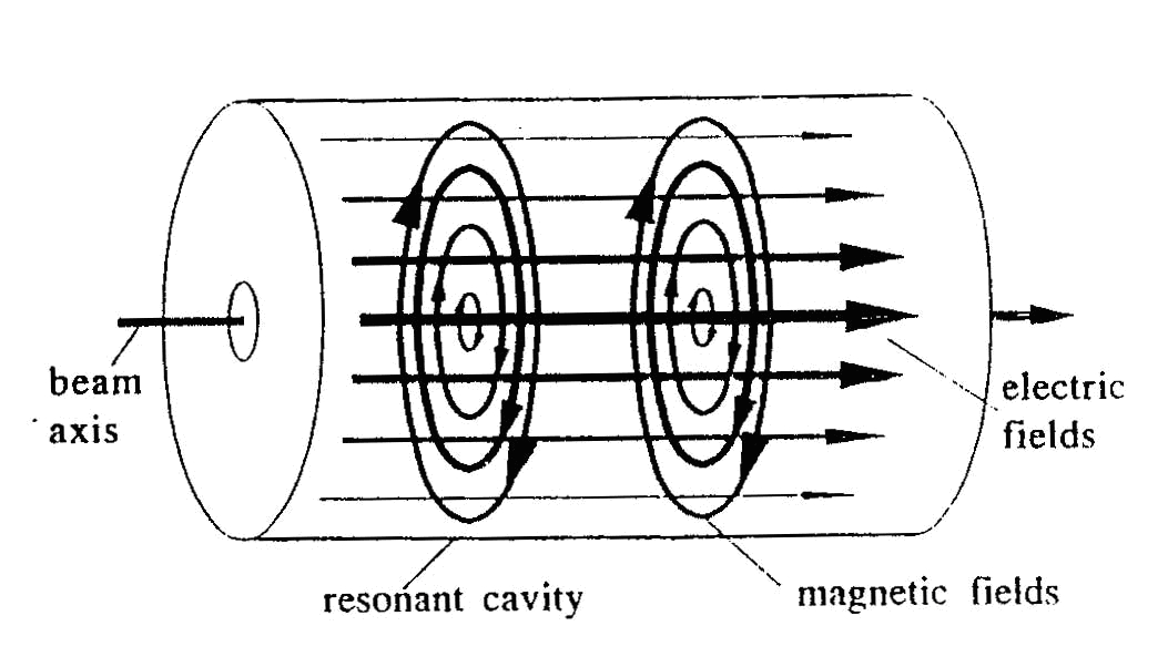
Figure 1: Electric and magnetic fields for the TM₀₁₀ mode inside a pill-box cavity.

Other resonant modes that are sometimes used are the TE₀₁₁ mode and the TM₁₁₀ mode. The first of these has a zero electric field on the cavity surface and is used to study the surface resistance of superconductors in RF magnetic fields. The second has a transverse component of the electric field on axis, tilting the beam, which is sometimes necessary in collider accelerators in order to provide a head-on collision between two beams and thereby increase the luminosity. The deflecting TM₁₁₀ mode has also been used in an SRF separator cavity to separate beams of different particles [Citron1979].

Although the resonant frequency of the TM₀₁₀ mode does not depend on the pill-box length, L, the following condition for synchronism between the beam and the electric field in the cavity sets the cavity length:

$$L=\beta c\frac{T_{\mathrm{RF}}}{2},$$ (3)

where $\beta$ is the speed of the particle relative to the speed of light and $T_{\mathrm{RF}}=2\pi/\omega_{0}$ is the period of oscillation of the RF field. The condition imposed by Eq. (3) assures that, as an example, a bunch of relativistic electrons entering the cavity at time $t=0$, when $E_{z}=0$, will experience the maximum acceleration as they travel along the cavity axis.

2.1 Figures of merit

The accelerating field of the cavity, $E_{\mathrm{acc}}$, is defined as the ratio of the accelerating voltage, $V_{\mathrm{c}}$, divided by the cavity length. $V_{\mathrm{c}}$ is obtained by integrating the electric field at the particle’s position as it traverses the cavity:

$$E_{\mathrm{acc}}=\frac{V_{\mathrm{c}}}{L}=\frac{1}{L}\left|\int_{0}^{L}E_{z}(\rho=0,z)\mathrm{e}^{i\omega_{0}z/c}\,\mathrm{d}z\right|.$$ (4)

Other important parameters are the ratios of the peak electric and magnetic fields on the cavity surface divided by the accelerating field, $E_{\mathrm{p}}/E_{\mathrm{acc}}$ and $B_{\mathrm{p}}/E_{\mathrm{acc}}$, respectively, as they are related to practical limitations of a cavity’s performance, such as field emission and quench.

The power dissipated as heat in the cavity wall, $P_{\mathrm{c}}$, and the energy stored within its volume, U, are given by

$$P_{\mathrm{c}}=\frac{1}{2}\Re\left\{\int_{V}\mathbf{J}\cdot\mathbf{E}\,\mathrm{d}v\right\}=\frac{1}{2}\int_{S}R_{\mathrm{s}}|\mathbf{H}|^{2}\,\mathrm{d}a,$$ (5)

$$U=\frac{1}{2}\mu_{0}\int_{V}|\mathbf{H}|^{2}\,\mathrm{d}v.$$ (6)

The quality factor of the cavity, $Q_{0}$, is defined, in the same way as for any resonator, as the ratio of the energy stored divided by the energy dissipated in in one RF period:

$$Q_{0}=\frac{\omega_{0}U}{P_{\mathrm{c}}}=\frac{\omega_{0}\mu_{0}\int_{V}|\mathbf{H}|^{2}\,\mathrm{d}v}{\int_{S}R_{\mathrm{s}}|\mathbf{H}|^{2}\,\mathrm{d}a}.$$ (7)

$Q_{0}$ can be calculated from the Breit–Wigner resonance curve as the ratio of the resonant frequency, divided by the full width at half maximum, as shown in Fig. LABEL:fig:resonance.

Assuming that the surface resistance is uniform over the cavity surface and does not depend on the amplitude of the applied field, it is possible to define from Eq. (7) a geometry factor, G, that depends only on the cavity shape (but not its size) and that provides a direct relation between $Q_{0}$ and $R_{\mathrm{s}}$:

$$G=\frac{\omega_{0}\mu_{0}\int_{V}|\mathbf{H}|^{2}\,\mathrm{d}v}{\int_{S}|\mathbf{H}|^{2}\,\mathrm{d}a}=Q_{0}R_{\mathrm{s}}.$$ (8)

The assumptions on the definition of G are usually valid at low field amplitudes.

The figures of merit for the TM₀₁₀ mode in a pill-box cavity, calculated from the analytical fields of Eq. (2), are as follows: