A combined radio and GeV $\gamma$-ray view of the 2012 and 2013 flares of Mrk 421

Abstract

In 2012 Markarian 421 underwent the largest flare ever observed in this blazar at radio frequencies. In the present study, we start exploring this unique event and compare it to a less extreme event in 2013. We use 15 GHz radio data obtained with the Owens Valley Radio Observatory 40-m telescope, 95 GHz millimeter data from the Combined Array for Research in Millimeter-Wave Astronomy, and GeV $\gamma$-ray data from the Fermi Gamma-ray Space Telescope. The radio light curves during the flaring periods in 2012 and 2013 have very different appearances, both in shape and peak flux density. Assuming that the radio and $\gamma$-ray flares are physically connected, we attempt to model the most prominent sub-flares of the 2012 and 2013 activity periods by using the simplest possible theoretical framework. We first fit a one-zone synchrotron self-Compton (SSC) model to the less extreme 2013 flare and estimate parameters describing the emission region. We then model the major $\gamma$-ray and radio flares of 2012 using the same framework. The 2012 $\gamma$-ray flare shows two distinct spikes of similar amplitude, so we examine scenarios associating the radio flare with each spike in turn. In the first scenario, we cannot explain the sharp radio flare with a simple SSC model, but we can accommodate this by adding plausible time variations to the Doppler beaming factor. In the second scenario, a varying Doppler factor is not needed, but the SSC model parameters require fine tuning. Both alternatives indicate that the sharp radio flare, if physically connected to the preceding $\gamma$-ray flares, can be reproduced only for a very specific choice of parameters.

1 Introduction

Blazars are active galactic nuclei (AGN) that are variable over the entire electromagnetic spectrum. Their variability is enhanced due to Doppler-beamed emission from a relativistic jet pointing close to the line of sight. Blazars having featureless optical spectra or showing emission lines with equivalent width $<5$ Å are historically classified as BL Lacs (Stocke et al., 1991).

Markarian 421 (hereafter Mrk 421) is one of the best studied BL Lac objects. It is relatively nearby with a redshift of $z=0.031$ (Ulrich et al., 1975). It is classified as a high synchrotron peaked blazar (Abdo et al., 2010b) based on its spectral energy distribution (SED). It was the first blazar detected at TeV energies (Punch et al., 1992), and since then it has been the subject of numerous multi-wavelength campaigns (e.g., Aleksić et al., 2012; Abdo et al., 2011; Acciari et al., 2011; Horan et al., 2009; Donnarumma et al., 2009; Fossati et al., 2008; Rebillot et al., 2006; Tosti et al., 1998). The broad-band SED of Mrk 421 can often be modeled with a one-zone synchrotron self-Compton (SSC) model (Aleksić et al., 2012; Acciari et al., 2011; Abdo et al., 2011) or with lepto-hadronic models involving proton synchrotron radiation and/or photopion interactions (e.g., Böttcher et al., 2013; Mastichiadis et al., 2013; Dimitrakoudis et al., 2014).

Mrk 421 exhibits large variations in the TeV, GeV, X-ray, and optical wavebands (e.g., Acciari et al., 2011, 2009; Horan et al., 2009; Błażejowski et al., 2005), with correlated TeV and X-ray variations (e.g., Giebels et al., 2007; Fossati et al., 2008). The connection between the TeV and optical bands is less clear and more detailed time-dependent models are being developed to study the complex correlations (see e.g., Chen et al. 2011 for SSC modeling and Mastichiadis et al. 2013 for lepto-hadronic modeling).

In 2012 Mrk 421 underwent its largest radio flare ever observed at 15 GHz (Hovatta et al., 2012). The flare time-scale was faster and its amplitude larger than any other radio flare observed from this source in the past 30 years of observations with the University of Michigan Radio Astronomy Observatory monitoring program (Richards et al., 2013). The radio flare occurred about 40 d after a major flare was observed in the $\gamma$-ray band (D’Ammando & Orienti, 2012) by the Fermi Gamma-Ray Space Telescope (hereafter Fermi). Unfortunately Mrk 421 was close to the sun at the time of the radio flare so that only limited multi-wavelength coverage in addition to the radio and $\gamma$-ray bands exists, apart from a NuSTAR calibration observation that covered the early activity (Baloković et al., 2013). In the spring of 2013, Mrk 421 underwent another major high-energy flaring event in the X-ray to TeV energies (Cortina & Holder, 2013; Baloković et al., 2013; Paneque et al., 2013). About 60 d later, it was followed by fairly small amplitude radio flares in the radio and millimeter bands (Hovatta et al., 2013a).

In this paper we present the radio data obtained with the Owens Valley Radio Observatory (OVRO) 40-m telescope at 15 GHz, and 95 GHz data obtained with Combined Array for Research in Millimeter-Wave Astronomy (CARMA). We compare the radio variations with the $\gamma$-ray light curves obtained by Fermi, by performing a cross-correlation analysis on the full data sets available from 2008 to 2013. Based on our findings and the coincidence of historically rare extreme flares in the two bands, we assume that the events in the radio and $\gamma$-ray bands are physically connected. Under this assumption we aim to understand the extreme nature of the 2012 radio event by adopting a reasonable physical model with the smallest number of free parameters.

Our paper is organized as follows. We describe the observations and data reduction in Sect. 2. The light curves and cross-correlations between the different bands are shown in Sect. 3. We model the flares in Sect. 4, discuss our results in Sect. 5, and present our conclusions in Sect. 6. Throughout the paper we use a cosmology where $H_{0}=71~{}\mathrm{km}~{}\mathrm{s}^{-1}~{}\mathrm{Mpc}^{-1}$, $\Omega_{M}=0.3$, and $\Omega_{\Lambda}=0.7$ (e.g., Komatsu et al., 2009).

2 Observations

We present radio and $\gamma$-ray observations of the two flaring events observed in 2012 and 2013. We are especially concerned with the extreme 2012 radio event, whereas the 2013 flare is more typical of the radio variability observed in Mrk 421.

2.1 Radio observations

Mrk 421 was observed as part of the blazar monitoring program with the OVRO 40-m telescope (Richards et al., 2011). In this program, a sample of over 1800 AGN are observed twice per week at 15 GHz. Mrk 421 has been included since the beginning of the monitoring in late 2007.

The OVRO 40-m telescope uses off-axis dual-beam optics and a cryogenic high electron mobility transistor (HEMT) low-noise amplifier with a 15.0 GHz center frequency and 3 GHz bandwidth. The two sky beams are Dicke switched using the off-source beam as a reference, and the source is alternated between the two beams in an ON-ON fashion to remove atmospheric and ground contamination. A noise level of approximately 3–4 mJy in quadrature with about 2 per cent additional uncertainty, mostly due to pointing errors, is achieved in a 70 s integration period. Calibration is achieved using a temperature-stable diode noise source to remove receiver gain drifts and the flux density scale is derived from observations of 3C 286 assuming the Baars et al. (1977) value of 3.44 Jy at 15.0 GHz. The systematic uncertainty of about 5 per cent in the flux density scale is not included in the error bars. Complete details of the reduction and calibration procedure are given in Richards et al. (2011).

For comparison and to fill gaps in the OVRO sampling, we also consider the 37 GHz light curve obtained by the Metsähovi Radio Observatory. These observations were made with the 13.7-m radome-enclosed telescope using a 1 GHz-bandwidth dual beam receiver centered at 36.8 GHz. A detailed description of the data reduction and analysis is given in Teräsranta et al. (1998). As the uncertainty in the data points is much larger than in the other bands, we do not include the data in any subsequent modeling.

2.2 Millimeter-band observations

Since February 2013, Mrk 421 was observed $1-3$ times per week with CARMA as a part of the MARMOT blazar monitoring project. The observations were made using the eight 3.5 m telescopes of the array with a central frequency of 95 GHz and a bandwidth of 7.5 GHz. The data were reduced using the MIRIAD (Multichannel Image Reconstruction, Image Analysis and Display) software (Sault et al., 1995), including standard bandpass calibration on a bright quasar. The amplitude and phase gain calibration was done by self-calibrating on Mrk 421. The absolute flux calibration was determined from a temporally nearby observation (within a day) of the planets Mars, Neptune or Uranus, whenever possible. Otherwise the quasar 3C 273 was used as a secondary calibrator. The estimated absolute calibration uncertainty of 10 per cent is not included in the error bars.

2.3 Gamma-ray data

The $\gamma$-ray data were obtained with the Large Area Telescope (LAT) aboard Fermi, which observes the entire sky every 3 hours at energies of $0.1-300$ GeV (Atwood et al., 2009). The publicly available reprocessed Pass 7 data were downloaded and analysed using the Fermi ScienceTools software package version v9r32p5. The data were binned using the adaptive binning method of Lott et al. (2012). The uneven bin size was determined in such a way that the statistical error in each flux measurement is $\sim$15 per cent We used the instrument response functions P7REP_SOURCE_V15, Galactic diffuse emission model “gll_iem_v05.fits” and isotropic background model “iso_source_v05.txt”. Source class photons (evclass=2) within 15^∘ of Mrk 421 were selected, with a zenith angle cut of 100^∘ and a rocking angle cut of 52^∘.

Once the bins were defined, the photon fluxes in the energy range of 0.1 - 200 GeV were calculated using unbinned likelihood and the tool gtlike with the Minuit optimizer. All sources within 15^∘ of Mrk 421 were included in the source model with their spectral parameters, except the flux, frozen to the values determined in the 2nd Fermi LAT catalog (2FGL; Nolan et al. 2012). For sources more than 10^∘ from Mrk 421 we also froze the fluxes to the 2FGL value. The 10 per cent systematic uncertainty below 100 MeV, decreasing linearly in Log(E) to 5 per cent in the range between 316 MeV and 10 GeV and increasing linearly in Log(E) up to 15 per cent at 1 TeV (Ackermann et al., 2012) is not included in the error bars. For the purpose of the modeling presented in Sect. 4, we also obtained the energy fluxes, with a power-law spectral model where the index is frozen to the 2FGL catalog value of $\Gamma=1.77$.

3 Light curves

The radio, millimeter and $\gamma$-ray light curves are shown in Fig. 1. They cover the time range since the beginning of the Fermi mission in August 2008 (MJD 54688) until the end of October 2013 (MJD 56610). The light curves illustrate the unusual nature of the 2012 flare (flare 1) in both radio and $\gamma$ rays, that lasted from May 2012 until October 2012 (MJD 56060 - 56225). This is a unique event, especially in the radio band where such fast and prominent flares have not been observed before in Mrk 421. The 2013 flare (flare 2) from March 2013 until November 2013 (MJD 56350-56610), although prominent, is much broader and of lower amplitude.

Figure 1: From top to bottom: light curves of Mrk 421 in $\gamma$ rays from Fermi LAT, radio 15 GHz from OVRO, 37 GHz from Metsähovi, and 95 GHz from CARMA. The light curves span a time period from August 2008 until November 2013, except for the CARMA light curve that starts in February 2013. The solid lines indicate the time range used to model the 2012 flare from 13 May 2012 (MJD 56060) until 25 October 2012 (MJD 56225). The dashed lines indicate the time range for the 2013 flare from 9 March 2013 (MJD 56360) until 14 November 2013 (MJD 56610). Because of the larger uncertainties in the data, the 37 GHz light curve is not used in any subsequent modeling.

A full cross-correlation analysis between more than four years of OVRO and LAT data was done by Max-Moerbeck et al. (2014b). They used weekly binned $\gamma$-ray light curves and data from 2008 until November 2012, including the rapid 2012 flare. They found a peak in the discrete correlation function (DCF), with the $\gamma$ rays leading the radio by $40\pm 9$ d. The significance of this correlation was between 96.16 and 99.99 per cent depending on the power spectral density (PSD) model used for the light curves, with a best-fitting value of 98.96 per cent. For details of the significance estimation, see Max-Moerbeck et al. (2014a). We repeated the cross-correlation analysis using the extended light curves considered here, and found that the DCF shows a broad peak ($\sim$ 30 d). In particular, the time delay ranges from 40 to 70 d with $\gamma$ rays leading, consistent with the estimate from Max-Moerbeck et al. (2014b). The significance of the peak was from 91.90 to 99.99 per cent, with a best fit value of 97.36 per cent, depending on the PSD model. The difference compared to the exact value derived by Max-Moerbeck et al. (2014b) is because they only considered the maximum of the DCF, while the peak itself is broad.

Recently, Emmanoulopoulos et al. (2013) introduced a method for simulating light curves, which also accounts for their flux distribution. This is more appropriate in the $\gamma$-ray light curves, as the light curves have a non-Gaussian photon flux distribution. Using this method, the significance of the correlation increases to 99.82 per cent, when using the best-fitting PSD. In the rest of the paper, we will thus assume that the major flares in radio and $\gamma$ rays are physically connected.

The $\gamma$-ray flares in both 2012 and 2013 have significant sub-structure, as already shown in Fig. 1 (top panel). If we also consider the broadness of the DCF peak, it becomes unclear which $\gamma$-ray spike of the overall flare is most plausibly associated with the radio peaks. Therefore, we consider both alternatives in our modeling.

3.1 The flare of 2012

On 16 July 2012 (MJD 56124) the $\gamma$-ray flux reached the highest value since the start of the Fermi mission (D’Ammando & Orienti, 2012). The $\gamma$-ray flux increased by a factor of three from $(3.4\pm 0.6)\times 10^{-7}$ ph cm^-2 s^-1 to $(1.1\pm 0.2)\times 10^{-6}$ ph cm^-2 s^-1 within seven days. The flare appears double peaked with the second flare peaking on 15 August 2012 (MJD 56154) at a flux of $(9.5\pm 0.1)\times 10^{-7}$ ph cm^-2 s^-1. The total duration of the flaring event was about 60 d. The OVRO 15 GHz light curve exhibits a fast rise which leads to an increase of the flux density by a factor of about two, i.e. from 0.6 to 1.1 Jy, in the period 6 August 2012 – 21 September 2012. This flux density is higher than any flux density measured at 15 GHz in the OVRO program or during the preceding 30-plus years of monitoring with the University of Michigan Radio Astronomy Observatory (Richards et al., 2013).

At the time of the first $\gamma$-ray peak there is a gap in the OVRO 15 GHz light curve. Thus, a double peaked radio flare cannot be excluded a priori. However, a higher frequency radio light curve observed at 37 GHz at Metsähovi Radio Observatory (third panel from the top in Fig. 1) shows only a single flare during 2012. Given the spectral proximity of the two radio bands and the similar features in the two light curves, it is safe to assume that the OVRO sampling does not miss a peak at the beginning of the event. Because of the larger statistical uncertainties in the 37 GHz data, we do not include them in our subsequent analysis as they would not add additional constraints on the modeling.

In order to obtain a better estimate of the time delay between the $\gamma$-ray and 15 GHz light curves for this flare only, we use the DCF method over the time period of the flare ( Fig. 2, bottom panel). There are two peaks in the DCF which simply correspond to the delays between each of the spikes in the double-peaked $\gamma$-ray flare and the single radio flare. The DCF peaks are both consistent with the delay measurement we obtained for the full light curves. Although the correlation is stronger for the $\sim$40 d lag, the amplitude of the DCF peak at about $-70$ d is not low enough to justify exclusion of a possible association of the radio flare with first $\gamma$-ray spike. Thus, we will test both possibilities in Sect. 4.

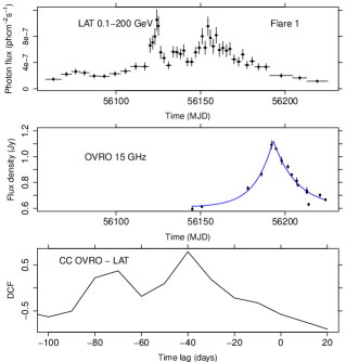
Figure 2: $\gamma$-ray flux (top) and 15 GHz flux density (middle) during the 2012 flare. The discrete correlation function between the two light curves is shown in the bottom panel. A negative time delay means that $\gamma$ rays are leading the radio. The (blue) solid line shows the exponential fit that is used to estimate the variability brightness temperature and Doppler factor. The residuals of the fit are on average less than 20 mJy. The time range in the figure corresponds to the solid lines in Fig. 1

.

We can estimate the Doppler boosting factor of the radio flare by assuming that the rise time of the flare corresponds to the light travel time across the emission region (Lähteenmäki & Valtaoja, 1999; Hovatta et al., 2009). We fit an exponential function of the form

$$S(t)=\Delta Se^{(t-t_{max})/t_{rise}},$$ (1)

to the light curve, where $\Delta S$ is the amplitude of the flare, $t_{max}$ is the peak location of the flare and $t_{rise}$ is the rise time of the flare. The decay time of the flare has been frozen to 1.3 times the rise time, as in Lähteenmäki & Valtaoja (1999). The fitting is done using the MultiNest Markov-Chain Monte Carlo (MCMC) algorithm (Feroz & Hobson, 2008; Feroz et al., 2009, 2013). As shown in Fig. 2 middle panel, an exponential function fits the 15 GHz flare fairly well. From the fit we obtain the rise time of the flare $t_{rise}=10.6\pm 0.5$ d and amplitude $\Delta S=0.52\pm 0.01$ Jy, where the uncertainties are estimated from the MCMC analysis.

Assuming an emission region with the geometry of a uniform disk, we can estimate the lower limit of the variability brightness temperature (Lähteenmäki et al., 1999; Hovatta et al., 2009)

$$T_{\rm var}=1.548\times 10^{-32}\frac{\Delta Sd_{L}^{2}}{\nu^{2}t_{rise}^{2}(1+z)},$$ (2)

where $d_{L}$ is the luminosity distance to the object in meters (here, $4.0\times 10^{24}~{}{\rm m}$), $z$ is the redshift, $\nu$ is the frequency in GHz, $t_{rise}$ is in days, and $\Delta S$ is in janskys. This gives us $T_{\rm var}=(5.2\pm 0.5)\times 10^{12}$K.

The variability brightness temperature is related to the Doppler factor, $\delta$, as $\delta=(T_{\rm var}/T_{\rm b,int})^{1/3}$, where $T_{\rm b,int}$ is the intrinsic brightness temperature (e.g., Lähteenmäki et al., 1999). As the variability brightness temperature estimate is a lower limit, the Doppler factor estimates are also lower limits. The largest uncertainty in the Doppler factor estimate comes from the uncertainty in the intrinsic brightness temperature and what method is used to estimate it. Assuming equipartition between the particles and magnetic field, $T_{\rm b,int}=10^{11}$K (Readhead, 1994). This results in a Doppler factor $\delta>3.7$. If we use a value of $T_{\rm b,int}=5\times 10^{10}$ K, as determined by Lähteenmäki et al. (1999), the Doppler factor is $\delta>4.7$.

We can further constrain the intrinsic brightness temperature by comparing the variability brightness temperature with the brightness temperature obtained via simultaneous Very Long Baseline Array (VLBA) observations (Lähteenmäki et al., 1999; Hovatta et al., 2013b). In order to study the parsec-scale jet structure after the 2012 flare we conducted 5 epochs of target-of-opportunity VLBA observations of Mrk 421 at several frequency bands (J. Richards et al. in preparation). The first one of these was taken on 12 October 2012 when the radio flare was already decaying. The brightness temperature estimate from the 15 GHz data is $T_{\rm VLBI}=5.2\times 10^{10}$ K (for a uniform disk), which depends on the Doppler factor as $\delta=T_{\rm VLBI}/T_{\rm b,int}$. We can then solve for the intrinsic brightness temperature by calculating $T_{\rm b,int}=\sqrt{T_{\rm VLBI}^{3}/T_{\rm var}}=5.2\times 10^{9}$ K. If we use this value for the intrinsic brightness temperature and the variability brightness temperature, we obtain $\delta>10$. Thus, we conclude that the lower limit of the Doppler factor is $\delta\sim 3-10$.

We note that the intrinsic brightness temperature obtained using the VLBA data is about $10-20$ times below the equipartition limit. We think the peak brightness temperature is likely higher than our estimate because by the time of the first VLBA epoch, the single-dish flux density had already declined by 30 per cent from the peak. Therefore it is likely that the true simultaneous brightness temperature from the VLBA observations is at least 30 per cent higher, because the core could have also been more compact, increasing the brightness temperature even further. Because of the strong dependence of $T_{\rm b,int}$ on $T_{\rm VLBI}$, any uncertainties in the VLBA parameters are magnified in the estimate of $T_{\rm b,int}$. A slightly higher $T_{\rm VLBI}$ would also agree with estimates from Lico et al. (2012), who found the core brightness temperature of Mrk 421 to be of the order of few times $10^{11}$ K, in agreement with equipartition arguments.

3.2 The flare of 2013

In April 2013, Mrk 421 was again flaring in the X-ray to TeV bands (Baloković et al., 2013; Paneque et al., 2013), reaching the highest levels ever observed at TeV energies (Cortina & Holder, 2013). Triggered by this activity, we began monitoring the source more frequently at CARMA.

The appearance of this flare was very different from the 2012 flare, both in the $\gamma$ rays and radio. In $\gamma$ rays the activity began in March 2013 reaching the highest peak on 14 April 2013 (MJD 56397). The flux increased from about $2\times 10^{-7}$ ph cm^-2 s^-1 to ($6.7\pm 0.9)\times 10^{-7}$ ph cm^-2 s^-1 over about 30 d and the flaring period consisted of several peaks over a total duration of about 100 d. At 15 GHz, the flux density began increasing in April 2013 from about 0.6 Jy to its peak of 0.77 Jy on 18 June 2013 (MJD 56461). Similarly, at 95 GHz the flux density increased from about 0.5 Jy to a peak of 0.71 Jy on 8 June 2013 (MJD 56451).

The DCFs between all the bands are shown in Fig. 3. The highest correlation is found for the 15 and 95 GHz data, with a peak at a delay of about $-10$ to $-20$ d, with 95 GHz leading. The time delays between the CARMA (OVRO) and LAT data can only be estimated at about $-60$ d ($-70$ d) because of the broad peaks of the DCF. These estimates are, however, compatible with the broad peak obtained from our cross-correlation analysis of the full light curves, and thus we assume that the events are physically connected in the radio and $\gamma$-ray bands.

Figure 3: Top: Light curves at $\gamma$ rays (left), 95 GHz (middle), and 15 GHz (right) during the 2013 flare. Bottom: Discrete correlation functions between the light curves. Negative time delay means that higher frequency emission ($\gamma$-ray or 95 GHz) is leading. The time range corresponds to the dashed lines in Fig. 1.

4 Conditions in the flaring region

In this section we attempt to explain the rough features of the 2012 and 2013 flaring periods, e.g., time delays between various energy bands, peak fluxes and pulse profiles, by adopting the simplest possible theoretical framework (the single zone SSC model), together with a minimum set of free parameters. In particular, we restrict our modeling to the major flares observed in the periods of MJD 56060-56225 and MJD 56360-56610, which are denoted as “flare 1” and “flare 2”’ in Sect. 3 (see Fig. 1), while modeling of the smaller amplitude variability seen in both bands lies out of the scope of this work. As the ‘goodness’ of the fits was not the main point of interest here, we did not attempt a detailed parameter space search for finding the set with the best $\chi^{2}$ value.

Based on the long-term radio light curve shown in Fig. 1, the 2013 radio and millimeter-band flares are more typical of blazar radio emission than the 2012 radio flare: they are less sharp, have a decay timescale larger than their rise timescale, and the flux density increases by no more than a factor of $\sim 1.4$ in both the radio and millimeter bands. We start our analysis with the 2013 flaring events in the context of a typical SSC model. Then, we highlight the differences between the 2012 and 2013 radio flares and discuss possible modifications within the same framework that may explain the 2012 data. Our main goal is to investigate what conditions are required to produce this extreme and unique radio flare. As already discussed in Sect. 3, we assume that the events in the radio and $\gamma$-ray bands are physically connected. We note that, in what follows, we ignore the small differences between quantities measured in the observer frame and the source frame since $1+z\simeq 1$.

4.1 The $\gamma$-ray and radio flares of 2013

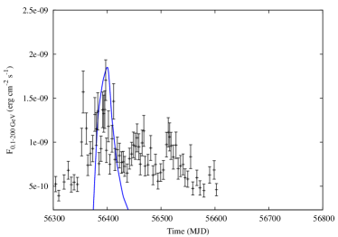
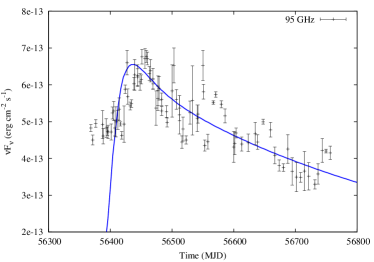
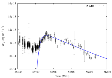
Figure 4: Fermi-LAT light curve (top), CARMA 95 GHz light curve (middle) and OVRO 15 GHz light curve (bottom). The results of the one-zone SSC model described in the text are shown with blue lines in all panels. The time range of the fit corresponds to the 2013 flare indicated by the dashed lines in Fig. 1.

Motivated by the fact that the CARMA and OVRO fluxes peak $\sim 60$ and 70 d after the $\gamma$-ray flare, respectively (Sect. 3.2), and by the fact that the decaying part of their light curve is approximately exponential, we applied the simple scenario where both the $\gamma$-ray and radio flares originate in the same region, which does not necessarily have the same physical conditions as the region responsible for the quiescent emission. We note that we do not attempt to model the sub-structure of the flares, but we only consider the highest peak in each band. In particular, we focus on the largest $\gamma$-ray flare, which peaks at MJD $\sim$56400. We also note that the DCF only shows a single peak for this flare, unlike in 2012 where we will consider multiple associations between flares.

In our scenario the $\gamma$-ray flare is produced by an instantaneous injection event of electrons having Lorentz factor $\gamma_{0}$ and emitting in $\gamma$ rays through Compton scattering of synchrotron photons (SSC). In particular, electrons are injected at $\tau=0$, which is set to be the time of the $\gamma$-ray flare, and then they are left to evolve via synchrotron and SSC cooling. In this context, the observed delays $t_{\rm h}\sim 60$ d and $t_{\ell}\sim 70$ d between the $\gamma$-ray and the radio flares at $\nu_{\rm h}=95$ GHz and $\nu_{\ell}=15$ GHz, respectively, correspond to the cooling timescale of electrons that have been injected at $\tau=0$ with Lorentz factor $\gamma_{0}$.

4.1.1 Analytical estimates

To define the size $R$ of the emitting region we choose as a typical variability timescale ($t_{\rm v}$) the one dictated by the $\gamma$-ray light curve. For the purpose of our analysis, we choose a variability timescale of $t_{\rm v}=20$ d based on the light curve. We note that the exact value is not critical as the estimate will be refined in the next section where we model the flares numerically. We find that $R\approx 2\times 10^{17}\ {\rm cm}\ \left(\delta/4\right)\left(t_{\rm v}/20\ {\rm d}\right)$, where we normalized the Doppler factor to 4 (see Sect. 3.1). In this framework, one can derive the magnetic field strength $B$ of the emission region as a function of the radio frequency $\nu_{\rm h}$, the observed time delay $t_{\rm h}$ and the Doppler factor $\delta$. Electrons that have been injected at $\tau=0$ with Lorentz factor $\gamma_{0}$ cool due to synchrotron losses and reach a Lorentz factor $\gamma_{\rm h}$. This can be found by solving the characteristic equation for synchrotron cooling and is given by

$$\gamma_{\rm h}=\frac{1}{1/\gamma_{0}+\alpha\delta t_{\rm h}}\approx\left(\alpha\delta t_{\rm h}\right)^{-1},$$ (3)

where $\alpha=(4/3)\sigma_{\rm T}cU_{\rm B}/m_{\rm e}c^{2}$ and $U_{\rm B}=B^{2}/8\pi$ is the energy density of the magnetic field. The approximation holds as long as $\gamma_{0}\gg\gamma_{\rm h}$. Combining Eq. (3) with the characteristic synchrotron frequency $\nu_{\rm h}=\delta m_{\rm e}c^{2}b\gamma_{\rm h}^{2}/h$, where $b=B/B_{\rm cr}$, $B_{\rm cr}=4.4\times 10^{13}$ G, and $h=6.63\times 10^{-27}$ erg s is the Planck constant, we find that the required magnetic field strength of the region is

$$B\simeq 0.5\ {\rm G}\left(\frac{\nu_{\rm h}}{95\ {\rm GHz}}\right)^{-1/3}\left(\frac{\delta}{4}\right)^{-1/3}\left(\frac{t_{\rm h}}{60\ {\rm d}}\right)^{-2/3},$$ (4)

which depends most strongly on the time delay between the $\gamma$-ray and radio flares. Notice also that lower values of the Doppler factor favour stronger magnetic fields. The expected time delays for the two frequencies should satisfy the relation $t_{\ell}/t_{\rm h}=(\nu_{\rm h}/\nu_{\ell})^{1/2}$. This is roughly consistent with the observed values, since $\sqrt{\nu_{\rm h}/\nu_{\ell}}=2.5$ and $t_{\ell}/t_{\rm h}$ is in the range of $1-1.7$ based on the broad peaks in the time delays (see Fig. 3). The duration of a flare is also related to the magnetic field strength, since it depends on the electron cooling timescale. For a given frequency $\nu_{\rm h}\propto B\gamma^{2}_{\rm h}$ the full width at half maximum (FWHM) of a flare will scale roughly as $\propto B^{-2}\gamma_{\rm h}^{-1}\propto B^{-3/2}\nu_{\rm h}^{-1/2}$. Thus, for strong enough magnetic fields the duration of a flare even at low frequencies may be shortened significantly.

Assuming that the inverse Compton scattering occurs in the Thomson limit, which will be checked a posteriori, the typical energy of up-scattered photons is given by $E_{\gamma}\simeq(4/3)\delta m_{\rm e}c^{2}b\gamma_{0}^{4}$. Using the value of $B$ derived above, we find that the injection Lorentz factor of electrons is $\gamma_{0}\simeq 2\times 10^{4}\left(E_{\gamma}/4\ {\rm GeV}\right)^{1/4}\left(\delta/4\right)^{-1/4}\left(B/0.5\ {\rm G}\right)^{-1/4}$, where we chose $E_{\gamma}=4$ GeV as a representative value for the energy of $\gamma$-ray photons. Because of the weak dependence of $\gamma_{0}$ on $E_{\gamma}$, a different choice of the $\gamma$-ray energy would not affect the derived value for the injection Lorentz factor. Increasing $E_{\gamma}$ by a factor of 50, for example, would increase $\gamma_{0}$ by only a factor of $\sim 2$. In principle, electrons could have been injected with $\gamma>\gamma_{0}$ and still produce the GeV flare, since they would very quickly cool to the value $\gamma_{0}$. In this case a contemporaneous TeV flare would also be expected, and indeed one was seen by the MAGIC and VERITAS instruments (Cortina & Holder, 2013). Having derived the expression for $\gamma_{0}$, which does not depend strongly on the parameters, we can now verify our earlier assumption that the Thomson limit applies. Since $b\gamma_{0}^{3}=0.09\left(\frac{B}{0.5\ {\rm G}}\right)^{1/4}\left(\frac{E_{\gamma}}{4\ {\rm GeV}}\right)^{3/4}\left(\frac{\delta}{4}\right)^{-3/4}<3/4$, we are safely in the Thomson regime. The derived values for the magnetic field strength and the Lorentz factor of injected electrons are reasonable and consistent with typical SSC models of high frequency peaked BL Lac objects, such as Mrk 421 (e.g., Abdo et al., 2011; Aleksić et al., 2012). Note, however, that here we adopted a low value for the Doppler factor implied by radio observations, in contrast to typical SED modeling where much larger values, e.g. $20-50$, are usually used (see e.g., Maraschi et al., 1999)

4.1.2 Numerical results

The required electron injection luminosity is determined numerically by fitting the observed energy fluxes. For this, we employed the numerical code described in Mastichiadis & Kirk (1995, 1997). Using as a stepping stone the values determined analytically in Sect. 4.1.1., we derive the following set of parameters: $R=10^{17}$ cm, $B=0.1$ G, $\delta=2.2$, $\gamma_{0}=2\times 10^{4}$ and the electron injection compactness $\ell_{\rm e}^{\rm inj}=1.6\times 10^{-2}$. This is defined as $\ell_{\rm e}^{\rm inj}=\sigma_{\rm T}RU_{\rm e}/m_{\rm e}c^{2}$ where $U_{\rm e}$ is the energy density of electrons at injection time as measured in the rest frame of the emission region and $\sigma_{T}=6.65\times 10^{-25}$ cm² is the Thomson cross section. Although our analytical estimates were based upon the hypothesis of instantaneous injection, here we find that an injection episode lasting $\sim R/c$, or equivalently $20$ d, is better in reproducing the observed flares.

Our results are illustrated in Fig. 4, where we use energy fluxes to facilitate comparison between the different bands. In the radio band, flux densities are converted to energy fluxes by multiplying by the observing frequency and converting to cgs units. The energy fluxes in the $\gamma$-ray band are obtained as described in Sect. 2. The model light curves can describe the radio observations fairly well, although the model $\gamma$-ray flare is slightly broader than the actual data. Still, the results of Fig. 4 are satisfactory given the small number of free parameters and the fact that we have not attempted to find the best fit (i.e., with the lowest $\chi^{2}$ value). The radio flares in both frequencies have wide pulse profiles and exhibit a slow exponential decay after their peak. Both of these features contrast with the sharpness and the symmetry of the 2012 flare. In the present scenario, the width of each flare is related to the cooling timescale of electrons emitting at the particular energy band and, thus, the radio flares are wider than the one in $\gamma$ rays (see Sect. 4.1.1.). The asymmetry of the pulse profiles at lower energies is a strong prediction of this model. Possible expansion of the flaring region and/or decay of the magnetic field would increase the predicted asymmetry.

For the derived parameters, the region is initially particle dominated with $U_{\rm e}\approx 0.18$ erg cm^-3 and $U_{\rm B}=4\times 10^{-4}$ erg cm^-3. The value of the Doppler factor derived here is approximately half of that obtained in Sect. 3.1 assuming equipartition. However, the large ratio $U_{\rm e}/U_{\rm B}\simeq 450$ derived from the values mentioned above would also imply a higher brightness temperature (e.g., Readhead, 1994) by a factor of $450^{1/8}\sim 2$ and thus a lower value of $\delta$ by a factor of $2^{-1/3}\sim 0.7$. Given that the fit shown in Fig. 4 is not unique, one could find parameters that would decrease the initial ratio $U_{\rm e}/U_{\rm B}$ and bring the emission region closer to an equipartition state. By assuming that a fraction $\eta_{\rm rad}$ of the injected luminosity in electrons is radiated as $\gamma$ rays, i.e. $\eta_{\rm rad}\ell_{\rm e}^{\rm inj}=L_{\gamma}^{\rm obs}\sigma_{\rm T}/4\pi R\delta^{4}m_{\rm e}c^{3}$, and using the definition of $\ell_{\rm e}^{\rm inj}$ as well as the equations for $R$ and $B$ in Sect. 4.1.1., we find that

$$\frac{U_{\rm e}}{U_{\rm B}}\simeq F_{0}\left(\frac{\eta_{\rm rad}}{0.1}\right)^{-1}\!\!\left(\frac{\delta}{4}\right)^{-16/3}\!\!\left(\frac{\nu_{\rm h}}{95\ {\rm GHz}}\right)^{2/3}\left(\frac{t_{\rm h}}{60\ {\rm d}}\right)^{4/3}\left(\frac{t_{\rm v}}{20\ {\rm d}}\right)^{-2},$$ (5)

where $F_{0}\equiv F_{\gamma}^{\rm obs}/2\times 10^{-9}$ erg cm^-2 s^-1. The ratio of energy densities depends strongly on the Doppler factor. Thus, searching for possible fits with a slightly higher value of the Doppler factor, e.g., $\delta\simeq 7$, would bring down the ratio from 450 to close to unity and would ensure rough equipartition between the particles and magnetic field at injection.

4.2 The $\gamma$-ray and radio flares of 2012

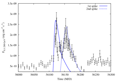
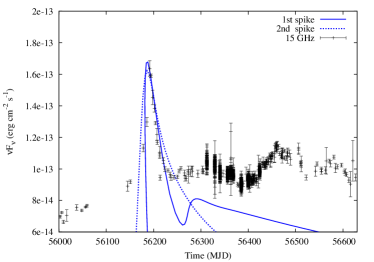
Figure 5: Fermi-LAT light curve (left) and OVRO 15 GHz light curve (right) in energy flux units along with the light curves (blue lines) obtained from the model. Solid and dashed lines demonstrate the model results, if the radio flare is associated with the first and second spikes of the $\gamma$-ray flare, respectively. A different x-axis range is used in the right panel to show the extended model light curve more clearly.

The 2012 radio flare is a unique event not only because of its large flux increase but also because of its symmetric pulse profile, which resembles flares at higher energies where the corresponding radiating particles cool efficiently. According to the cross-correlation analysis presented in Sect. 3.1, the 2012 radio flare may be associated with either the first or second spike of the $\gamma$-ray flare (see Figs. 1 and 2). We investigate both possibilities under the assumption that there is indeed a physical connection between the extreme radio and $\gamma$-ray flares. For this we begin with the parameters we derived for the 2013 “typical” flare, and examine two alternative scenarios. These include changes of the Doppler factor and magnetic field strength, since both parameters are related to the time delay (see Eq. 4) and to the pulse profile (see Sect. 4.1.1.). We emphasize that in both scenarios we attempt to introduce minimal changes to the parameters. As before, we do not consider the small-amplitude sub-structure of the flares.

4.2.1 Association of the radio flare with the first $\gamma$-ray spike

We first investigate the possibility that the radio flare is associated with the narrower first spike of the $\gamma$-ray flare, which peaks at $\sim$56133 MJD. In order to do this, we use the same parameter set as derived for the 2013 flare, but add variations in the Doppler beaming to the model. Such changes could occur if the emission region moves on a curved trajectory with a changing viewing angle, or if the bulk Lorentz factor of the emission region changes. Varying Doppler factors have been previously used to explain radio spectral variations in, for example, S5 0716+714 (Rani et al., 2013). The Doppler factor $\delta$ is modeled as

$$\delta(\tau)=\delta_{0}\left(1+g(\tau)\cos(2\pi\tau/P)\right),$$ (6)

where $\delta_{0}=2.1$, $\tau$ is the time in the comoving frame in $R/c$ units, $P=5.4$ is the period of the variation in $R/c$ units and $g(\tau)$ is the function

$$g(\tau) = 0.3,\ {\rm for}\ \tau<\tau_{\rm br}$$ (7)

$$g(\tau) = 0.3e^{-(\tau-\tau_{\rm br})/T},\ {\rm for}\ \tau\geq\tau_{\rm br},$$ (8)

with $\tau_{\rm br}=1.2P$ and $T=0.2P$.

The model-derived pulse profiles are shown in Fig. 5 with blue solid lines. Although the cooling timescale of electrons emitting at radio frequencies is long compared to those emitting initially at $\gamma$ rays, the shape of the radio flare (right panel in Fig. 5) is well reproduced here, because of the change in the Doppler factor, which does not allow the observer to see the typical wide pulse profile (see e.g., Fig. 4). The effect of the variable $\delta$ on the $\gamma$-ray light curve is negligible because the radiating electrons at the time of injection have short cooling timescales. Note that the exponentially decaying amplitude in the variation of $\delta$ is required in order to avoid any excess of the radio emission following the extreme flare.

Assuming that the change in the Doppler factor is caused by small variations in the viewing angle $\theta$ while the Lorentz factor remains constant at $\Gamma=10$, no extreme variations in either $\delta$ or the angle $\theta=\cos^{-1}\left(\beta^{-1}\left(1-(\Gamma\delta)^{-1}\right)\right)$ are required. In particular, $\delta$ and $\theta$ change by less than $28$ and $22$ per cent, respectively, relative to their average values.

The fact that the necessary parameter changes are small make this scenario plausible and attractive. However, if we attempt to interpret the second spike of the $\gamma$-ray flare in the same framework, then we cannot avoid the appearance of a radio flare $\sim$ 70 d later, i.e. at MJD 56220. Its absence implies one (or more) of the following: (i) a faster onset of the exponential decay of $\delta$; (ii) a different functional form for $\delta(\tau)$; (iii) different conditions in the emission region which suppress the 15 GHz emission, such as different magnetic field and/or size; (iv) a different framework for the second $\gamma$-ray spike.

Finally, the choice of a damped oscillator for modeling $\delta(\tau)$, albeit plausible, was not based on a physical picture. According to the discussion of Sect. 4.1.1., the FWHM of a flare depends on the magnetic field strength. Therefore, another alternative might be to adopt a stronger magnetic field for the emission region. Although a stronger magnetic field would lead to a shorter duration of the flare, an even lower value of the Doppler factor would be required in order to explain the observed time delay between the $\gamma$-ray and radio flares (see Eq. 4). Given that the value of the Doppler factor already lies at the low end of values consistent with observations, we do not examine this possibility in more detail.

4.2.2 Association of the radio flare with the second $\gamma$-ray spike

We now consider the scenario where the radio flare is associated with the second spike of the $\gamma$-ray flare. This scenario would arise naturally if the first $\gamma$-ray spike occurred when the emission region was still optically thick to radio emission. In this case, the time-delay between the $\gamma$-ray and radio flares is shorter than before, which, in our framework, suggests faster electron cooling. We searched, therefore, for reasonable fits using a stronger magnetic field than that adopted in Sect. 4.2.1, and obtained the following parameter set: $B=0.25$ G, $\delta=2.3$ and $\ell_{\rm e}^{\rm inj}=1.3\times 10^{-2}$. All other parameters, including the injection profile, are the same as before.

The resulting pulse profiles are shown in Fig. 5 with dashed blue lines. We find that the light curves obtained by the model are in rough agreement with the observations, with the radio light curve having a slightly longer decay timescale than is observed. In this scenario, even without Doppler factor variations, we obtain a sharper radio flare than the one in 2013 (see e.g. Fig. 4). Comparing these parameter values with the first scenario, we see that although we adjusted the numerical values for three parameters, only the magnetic field is significantly altered. It has increased by a factor of 2.5. We can compare the FWHM of the 15 GHz radio flares in 2012 and 2013 as obtained by our model (Figs. 4 and 5). We find their ratio to be $\Delta T_{2012}/\Delta T_{2013}\sim 0.16$, where $\Delta T$ denotes the duration at FWHM. This is comparable to the analytical estimate we can obtain from Eq. 4, $\Delta T_{2012}/\Delta T_{2013}\simeq\left(B_{2012}/B_{2013}\right)^{-3/2}\simeq\left(0.25/0.1\right)^{-3/2}=0.25$.

We note that this model is subject to tight constraints on its parameters. These must be adjusted to ensure: (i) the electron cooling timescale results in the observed delay between the $\gamma$-ray spike and the radio flare (see Eq. (4)); (ii) the cooling timescale of electrons radiating at the radio frequency is such that it explains the observed width of the pulse; and (iii) the synchrotron self-absorption frequency, which depends on $\ell_{\rm e}^{\rm inj}$, $B$ and $R$, is below the radio frequency where the extreme flare is observed. From the above it becomes clear that fine tuning of the parameters is required for this scenario to be viable.

5 Discussion

Unlike in many other blazars, prominent radio flares are rare in Mrk 421 and there are few examples where the radio flares have been modeled in detail. In 1997 a 22 GHz flare was observed with the Metsähovi Radio Observatory 14-m telescope (Tosti et al., 1998). The flare lasted about 200 d during which the flux density increased by a factor of two. The radio flare occurred 60 d after a large optical flare that also included very high optical polarization. Due to the high optical polarization during the flare, the authors interpreted the flare within the shock-in-jet model of Marscher & Gear (1985). The delay between the optical and radio bands was explained by opacity effects. While this model may explain the general features of the flares and the delay between optical and radio bands, more detailed modeling was not presented by Tosti et al. (1998).

In 2001 a simultaneous flare was observed at TeV, X-ray and 5 GHz radio bands (Katarzyński et al., 2003). The radio flux density increased by a factor of 1.5 and the flare lasted only for 15 d. The absence of time delays between the bands indicates that the emission region was optically thin even at radio frequencies. An instant injection of particles into the jet base was unable to explain the radio flares as the electrons would have cooled too much to generate significant flux density changes before reaching the optically thin regime for radio emission. Instead, detailed modeling of the flare suggested that it was caused by in-situ acceleration of electrons in a blob in the jet. The expansion of the blob explains the decay of the flare at all bands.

The 2013 flaring event was a more typical example of radio flares in Mrk 421, with a broad flare in the millimeter and centimeter bands (see Fig. 1 for the long-term behavior). Assuming that the events in the different bands are physically connected, we modeled the most prominent features of this event with a simple one-zone SSC model where an instantaneous injection of electrons produces a $\gamma$-ray flare. Then, as electrons cool because of synchrotron and SSC energy losses, they radiate at longer wavelengths and eventually produce the radio flares with a delay relative to the $\gamma$-ray flare. Within this context, we estimated the required magnetic field strength, the size of the emission region, and the Lorentz factor of electrons at injection. While the simple model presented here can describe the main features of the data satisfactorily, more information from simultaneous multi-wavelength observations is needed in order to discriminate between other possible models. For example, one could postulate a scenario where the delay between the $\gamma$-ray and radio flares is related to opacity effects, such as if the source were optically thick in radio frequencies at the time of the GeV flare but eventually became optically thin due to the expansion of the emission region or decay of the magnetic field (e.g., Fuhrmann et al., 2014). Although the coincident unprecedented events between the LAT and OVRO data suggests a physical connection of the high- and low-energy emission, models where two spatially separated emission regions are invoked (Błażejowski et al., 2005; Petropoulou, 2014) are still viable alternatives. We note that the 2013 flare occurred during a planned multi-wavelength campaign and Mrk 421 was observed regularly with numerous instruments at various frequency bands. Therefore we anticipate several dedicated studies of the behavior of Mrk 421 during this flare.

Even though the 2012 radio flare was more extreme, the Doppler factor inferred from the radio variability time-scale is fairly low, only about $3-10$. This is in accordance with the low observed apparent speeds obtained through radio interferometric observations where only subluminal speeds have been detected (e.g., Piner et al., 1999; Lico et al., 2012; Lister et al., 2013). Based on the jet brightness asymmetry, low observed apparent speeds, and low brightness temperature of the core component, Lico et al. (2012) estimate the radio Doppler beaming factor to be about 3, consistent with our estimate. If simultaneous X-ray or TeV data were available, we could estimate a minimum Doppler factor by demanding the source to be optically thin to the highest energy emitted photon (e.g., Dondi & Ghisellini, 1995). From previous TeV flares of Mrk 421 it has been estimated that the minimum Doppler factor required for the TeV emission to be optically thin is $\sim 10$ (Celotti et al., 1998), which is marginally higher than the value obtained from our radio data when equipartition is assumed.

Preliminary analysis of our follow-up VLBA observations indicate that the component speeds were consistent with subluminal motion even after the major flare (Richards et al., 2013). If we take the fastest observed jet speed, $\beta_{\mathrm{app}}=0.28c$, obtained from several years of monitoring at 15 GHz with the VLBA (Lister et al., 2013), we can estimate the jet Lorentz factor as

$$\Gamma_{\mathrm{var}}=\frac{\beta_{\mathrm{app}}^{2}+\delta_{\mathrm{var}}^{2}+1}{2\delta_{\mathrm{var}}},$$ (9)

where $\delta_{\mathrm{var}}$ is the Doppler factor inferred from the variability time-scales. This results in a Lorentz factor of $\Gamma_{\mathrm{var}}\sim 1.7-5$. Similarly, we can estimate the viewing angle of the jet to be

$$\theta_{\mathrm{var}}=\arctan\frac{2\beta_{\mathrm{app}}}{\beta_{\mathrm{app}}^{2}+\delta_{\mathrm{var}}^{2}-1},$$ (10)

resulting in $\theta_{\mathrm{var}}\sim 0.3-4^{\circ}$. As noted by Lico et al. (2012), it is unlikely that the component speeds resemble the flow speed in Mrk 421 because unreasonably small viewing angles would be required to explain the beaming estimates from the jet/counter-jet ratio. In this case the above equations would not be valid for estimating the true Lorentz factor and viewing angles. However, they find a viable scenario for Mrk 421 with a structured jet, where the viewing angle is between $2^{\circ}$ and $5^{\circ}$, and the Lorentz factor of the radio emitting region about 1.8, in agreement with our estimates.

One of the long-standing problems in modeling of the high synchrotron peaked blazars is the large discrepancy between the Doppler factor values inferred from radio observations and those obtained by SED modeling, with the former being usually $\lesssim 10$ (e.g., Piner et al., 1999; Lister et al., 2013) and the latter lying in the range $\sim 20-50$ (e.g., Maraschi et al., 1999; Abdo et al., 2011). Several alternatives have been explored to explain this well-known “Doppler factor crisis”, such as a structured jet (Ghisellini et al., 2005), a decelerating jet (Georganopoulos & Kazanas, 2003), and a jet-in-jet model (Giannios et al., 2009). In the structured jet model the high-energy emission comes from a fast spine of the jet while the radio emission is produced in a slower sheath (Ghisellini et al., 2005). This model is favored by observations of limb brightening of the Mrk 421 jet at 43 GHz (Piner et al., 2010).

In the present work, where we have adopted a single-zone emission model, we attempted to avoid a large discrepancy between the Doppler factor values inferred from the observations and those used in the modeling of the flares. However, one could relax this condition and search for possible fits to both the radio and $\gamma$-ray flares with $\delta\gtrsim 20$. One can estimate the effect of a higher $\delta$ on our results by inspection of the analytical expressions derived in Sect. 4.1.1. In particular, we find that $R\propto\delta$, $B\propto\delta^{-1/3}$, $\gamma_{0}\propto\delta^{-1/6}$, $U_{\rm e}/U_{\rm B}\propto\delta^{-16/3}$ and FWHM$\propto\delta^{1/2}$, where we assumed that the radio observing frequencies and their time-delays with respect to the $\gamma$-ray flare are fixed. On the one hand, choice of a higher $\delta$ would require a weaker magnetic field, a larger emission region and would reduce the ratio of particle to magnetic energy densities (see discussion in Sect. 4.1.2). On the other hand, the model light curves would be wider than those presented in Fig. 4, since the FWHM would increase. This is a direct result of the longer electron cooling timescale due to the weaker magnetic field. We conclude, therefore, that values $\gtrsim 20$ are less plausible for the modeling of both the radio and $\gamma$-ray flares. Another possibility is to assume a high Doppler factor value for the $\gamma$-ray flare alone and a low value for the radio flares. Because a single-zone model only contains a single Doppler factor, this parameter would need to change rapidly between the two flares. This scenario would require the Doppler factor to drop by $\gtrsim 10$ between the $\gamma$-ray and radio flare within a period of $t_{\rm h}=60$ d, which is much larger than the modest variations applied in the modeling of the 2012 flares.

The 2012 $\gamma$-ray flare had two prominent spikes, and we used these to investigate the physical conditions required to produce the extreme radio event. By using the 2013 model parameters as a starting point and introducing as few modifications as possible, we considered two possible scenarios. These result from the association of the radio flare with the first or second $\gamma$-ray spikes. Under the assumption of a physical connection between the radio flare and the first $\gamma$-ray spike, we showed that the addition of a varying Doppler beaming factor to a one-zone SSC model with fairly typical parameters can explain the observed sharp radio flare. The SSC model would otherwise produce too broad a radio flare, similar to the 2013 event (see Figs. 4-5). Although this scenario succeeds in explaining the radio flare, it results in a wider $\gamma$-ray pulse profile than is observed (solid lines in Fig. 5). Moreover, it is difficult to explain the lack of a second peak in the radio light curve, as discussed in the end of Sect. 4.2.1. Nonetheless, a varying Doppler beaming factor is not unreasonable. An adequate variation could result from, e.g., a modest change in the Lorentz factor or the viewing angle. In the latter case, the sharp flare would occur when the direction of motion of the emission region crosses very near to the line of sight to the observer. Similar models with curved emission region trajectories have been suggested for other blazars as well (e.g., Marscher et al., 2008, 2010; Abdo et al., 2010a; Rani et al., 2013; Aleksić et al., 2014; Molina et al., 2014). These models assume that either the emission feature moves on a helical trajectory due to an ordered helical magnetic field (Marscher et al., 2008, 2010; Molina et al., 2014), or that there is an actual bend in the jet (Abdo et al., 2010a; Aleksić et al., 2014).

In our second scenario, we considered the possibility that the radio flare is associated with the second, broader $\gamma$-ray spike. In this case, the short duration of the radio flare and the shorter time delay between the radio and $\gamma$-ray flares imply faster electron cooling, and thus a stronger magnetic field than the one used in the first scenario. We found indeed that a viable model is achieved by increasing the magnetic field strength by a factor of 2.5. Fig. 5 shows that the model light curve (dashed lines) describes well the $\gamma$-ray data, although the modeled radio flare is now not quite as sharp as the observed one. In this scenario, the first $\gamma$-ray spike would have to be unassociated with the radio event, perhaps by occurring closer to the black hole where the emission region is optically thick for radio emission.

6 Conclusions

We have obtained radio, millimeter and $\gamma$-ray light curves of Mrk 421 during the flaring activity in 2012 and 2013. In July 2012, Mrk 421 exhibited the largest $\gamma$-ray flare observed by Fermi since the beginning of its mission. About $40-70$ d later, the largest ever 15 GHz flare was observed. The flare rise time determined from an exponential fit was just $10.6\pm 0.5$ d, which is extreme compared to previous radio flares observed in the source. This implies a variability Doppler factor $\delta\sim 3-10$. In 2013 Mrk 421 underwent major $\gamma$-ray flaring again, followed by radio and millimeter flares about 60 d later. Under the assumption that the events in the different bands are physically connected we have modeled the variations with the simplest possible theoretical model, with the main goal of explaining the extreme radio flare in 2012. Starting with the less extreme 2013 flare, we obtained a one-zone SSC model that could explain the main features of the flares reasonably well. The 2012 $\gamma$-ray flare was double peaked, and by modeling the radio flare as connected to each peak in turn, we were able to reproduce the radio flare with either a varying Doppler factor, or an increased magnetic field strength. In both cases several specific conditions in the jet need to be fulfilled for the models to be viable, showing the extreme and unique nature of the 2012 event.

References

- Abdo et al. (2010a) Abdo A. A. et al., 2010a, Nature, 463, 919
- Abdo et al. (2010b) Abdo A. A. et al., 2010b, ApJ, 716, 30
- Abdo et al. (2011) Abdo A. A. et al., 2011, ApJ, 736, 131
- Acciari et al. (2009) Acciari V. A. et al., 2009, ApJ, 703, 169
- Acciari et al. (2011) Acciari V. A. et al., 2011, ApJ, 738, 25
- Ackermann et al. (2012) Ackermann M. et al., 2012, ApJS, 203, 4
- Aleksić et al. (2012) Aleksić J. et al., 2012, A&A, 542, A100
- Aleksić et al. (2014) Aleksić J. et al., 2014, A&A, 567, A41
- Atwood et al. (2009) Atwood W. B. et al., 2009, ApJ, 697, 1071
- Baars et al. (1977) Baars J. W. M., Genzel R., Pauliny-Toth I. I. K., Witzel A., 1977, A&A, 61, 99
- Baloković et al. (2013) Baloković M., Furniss A., Madejski G., Harrison F., 2013, The Astronomer’s Telegram, 4974, 1
- Baloković et al. (2013) Baloković M. et al., 2013, in European Physical Journal Web of Conferences. European Physical Journal Web of Conferences, Vol. 61, p. 4013
- Błażejowski et al. (2005) Błażejowski M. et al., 2005, ApJ, 630, 130
- Böttcher et al. (2013) Böttcher M., Reimer A., Sweeney K., Prakash A., 2013, ApJ, 768, 54
- Celotti et al. (1998) Celotti A., Fabian A. C., Rees M. J., 1998, MNRAS, 293, 239
- Chen et al. (2011) Chen X., Fossati G., Liang E. P., Böttcher M., 2011, MNRAS, 416, 2368
- Cortina & Holder (2013) Cortina J., Holder J., 2013, The Astronomer’s Telegram, 4976, 1
- D’Ammando & Orienti (2012) D’Ammando F., Orienti M., 2012, The Astronomer’s Telegram, 4261, 1
- Dimitrakoudis et al. (2014) Dimitrakoudis S., Petropoulou M., Mastichiadis A., 2014, Astroparticle Physics, 54, 61
- Dondi & Ghisellini (1995) Dondi L., Ghisellini G., 1995, MNRAS, 273, 583
- Donnarumma et al. (2009) Donnarumma I. et al., 2009, ApJ, 691, L13
- Emmanoulopoulos et al. (2013) Emmanoulopoulos D., McHardy I. M., Papadakis I. E., 2013, MNRAS, 433, 907
- Feroz & Hobson (2008) Feroz F., Hobson M. P., 2008, MNRAS, 384, 449
- Feroz et al. (2009) Feroz F., Hobson M. P., Bridges M., 2009, MNRAS, 398, 1601
- Feroz et al. (2013) Feroz F., Hobson M. P., Cameron E., Pettitt A. N., 2013, ArXiv e-prints 1306.2144
- Fossati et al. (2008) Fossati G. et al., 2008, ApJ, 677, 906
- Fuhrmann et al. (2014) Fuhrmann L. et al., 2014, MNRAS, 441, 1899
- Georganopoulos & Kazanas (2003) Georganopoulos M., Kazanas D., 2003, ApJ, 594, L27
- Ghisellini et al. (2005) Ghisellini G., Tavecchio F., Chiaberge M., 2005, A&A, 432, 401
- Giannios et al. (2009) Giannios D., Uzdensky D. A., Begelman M. C., 2009, MNRAS, 395, L29
- Giebels et al. (2007) Giebels B., Dubus G., Khélifi B., 2007, A&A, 462, 29
- Horan et al. (2009) Horan D. et al., 2009, ApJ, 695, 596
- Hovatta et al. (2009) Hovatta T., Valtaoja E., Tornikoski M., Lähteenmäki A., 2009, A&A, 494, 527
- Hovatta et al. (2012) Hovatta T., Richards J. L., Aller M. F., Aller H. D., Max-Moerbeck W., Pearson T. J., Readhead A. C. S., 2012, The Astronomer’s Telegram, 4451, 1
- Hovatta et al. (2013a) Hovatta T., Baloković M., Richards J. L., Max-Moerbeck W., Readhead A. C. S., 2013a, The Astronomer’s Telegram, 5107, 1
- Hovatta et al. (2013b) Hovatta T., Leitch E. M., Homan D. C., Wiik K., Lister M. L., Max-Moerbeck W., Richards L. J., Readhead A. C. S., 2013b, in European Physical Journal Web of Conferences. European Physical Journal Web of Conferences, Vol. 61, p. 6005
- Katarzyński et al. (2003) Katarzyński K., Sol H., Kus A., 2003, A&A, 410, 101
- Komatsu et al. (2009) Komatsu E. et al., 2009, ApJS, 180, 330
- Lähteenmäki & Valtaoja (1999) Lähteenmäki A., Valtaoja E., 1999, ApJ, 521, 493
- Lähteenmäki et al. (1999) Lähteenmäki A., Valtaoja E., Wiik K., 1999, ApJ, 511, 112
- Lico et al. (2012) Lico R. et al., 2012, A&A, 545, A117
- Lister et al. (2013) Lister M. L. et al., 2013, AJ, 146, 120
- Lott et al. (2012) Lott B., Escande L., Larsson S., Ballet J., 2012, A&A, 544, A6
- Maraschi et al. (1999) Maraschi L. et al., 1999, ApJ, 526, L81
- Marscher & Gear (1985) Marscher A. P., Gear W. K., 1985, ApJ, 298, 114
- Marscher et al. (2008) Marscher A. P. et al., 2008, Nature, 452, 966
- Marscher et al. (2010) Marscher A. P. et al., 2010, ApJ, 710, L126
- Mastichiadis & Kirk (1995) Mastichiadis A., Kirk J. G., 1995, A&A, 295, 613
- Mastichiadis & Kirk (1997) Mastichiadis A., Kirk J. G., 1997, A&A, 320, 19
- Mastichiadis et al. (2013) Mastichiadis A., Petropoulou M., Dimitrakoudis S., 2013, MNRAS, 434, 2684
- Max-Moerbeck et al. (2014a) Max-Moerbeck W., Richards J. L., Hovatta T., Pavlidou V., Pearson T. J., Readhead A. C. S., 2014a, MNRAS, 445, 437
- Max-Moerbeck et al. (2014b) Max-Moerbeck W. et al., 2014b, MNRAS, 445, 428
- Molina et al. (2014) Molina S. N., Agudo I., Gómez J. L., Krichbaum T. P., Martí-Vidal I., Roy A. L., 2014, A&A, 566, A26
- Nalewajko et al. (2014) Nalewajko K., Begelman M. C., Sikora M., 2014, ApJ, 789, 161
- Nolan et al. (2012) Nolan P. L. et al., 2012, ApJS, 199, 31
- Paneque et al. (2013) Paneque D., D’Ammando F., Orienti M., Falcon A., 2013, The Astronomer’s Telegram, 4977, 1
- Petropoulou (2014) Petropoulou M., 2014, A&A, 571, A83
- Piner et al. (1999) Piner B. G., Unwin S. C., Wehrle A. E., Edwards P. G., Fey A. L., Kingham K. A., 1999, ApJ, 525, 176
- Piner et al. (2010) Piner B. G., Pant N., Edwards P. G., 2010, ApJ, 723, 1150
- Punch et al. (1992) Punch M. et al., 1992, Nature, 358, 477
- Rani et al. (2013) Rani B. et al., 2013, A&A, 552, A11
- Readhead (1994) Readhead A. C. S., 1994, ApJ, 426, 51
- Rebillot et al. (2006) Rebillot P. F. et al., 2006, ApJ, 641, 740
- Richards et al. (2011) Richards J. L. et al., 2011, ApJS, 194, 29
- Richards et al. (2013) Richards J. L. et al., 2013, in European Physical Journal Web of Conferences. European Physical Journal Web of Conferences, Vol. 61, p. 4010
- Sault et al. (1995) Sault R. J., Teuben P. J., Wright M. C. H., 1995, in R.A. Shaw, H.E. Payne, J.J.E. Hayes, eds, Astronomical Data Analysis Software and Systems IV. Astronomical Society of the Pacific Conference Series, Vol. 77, p. 433
- Stocke et al. (1991) Stocke J. T., Morris S. L., Gioia I. M., Maccacaro T., Schild R., Wolter A., Fleming T. A., Henry J. P., 1991, ApJS, 76, 813
- Teräsranta et al. (1998) Teräsranta H. et al., 1998, A&AS, 132, 305
- Tosti et al. (1998) Tosti G. et al., 1998, A&A, 339, 41
- Ulrich et al. (1975) Ulrich M. H., Kinman T. D., Lynds C. R., Rieke G. H., Ekers R. D., 1975, ApJ, 198, 261