Abstract

Bayesian hierarchical clustering (BHC) is an agglomerative clustering method, where a probabilistic model is defined and its marginal likelihoods are evaluated to decide which clusters to merge. While BHC provides a few advantages over traditional distance-based agglomerative clustering algorithms, successive evaluation of marginal likelihoods and careful hyperparameter tuning are cumbersome and limit the scalability. In this paper we relax BHC into a non-probabilistic formulation, exploring small-variance asymptotics in conjugate-exponential models. We develop a novel clustering algorithm, referred to as relaxed BHC (RBHC), from the asymptotic limit of the BHC model that exhibits the scalability of distance-based agglomerative clustering algorithms as well as the flexibility of Bayesian nonparametric models. We also investigate the reducibility of the dissimilarity measure emerged from the asymptotic limit of the BHC model, allowing us to use scalable algorithms such as the nearest neighbor chain algorithm. Numerical experiments on both synthetic and real-world datasets demonstrate the validity and high performance of our method.

1 INTRODUCTION

Agglomerative hierarchical clustering, which is one of the most popular algorithms in cluster analysis, builds a binary tree representing the cluster structure of a dataset (Duda et al., 2001). Given a dataset and a dissimilarity measure between clusters, agglomerative hierarchical clustering starts from leaf nodes corresponding to individual data points and successively merges pairs of nodes with smallest dissimilarities to complete a binary tree.

Bayesian hierarchical clustering (BHC) (Heller and Ghahrahmani, 2005) is a probabilistic alternative of agglomerative hierarchical clustering. BHC defines a generative model on binary trees and compute the probability that nodes are merged under that generative model to evaluate the (dis)similarity between the nodes. Since this (dis)similarity is written as a probability, one can naturally decide a level, where to stop merging according to this probability. Hence, unlike traditional agglomerative clustering algorithms, BHC has a flexibility to infer a proper number of clusters for given data. The source of this flexibility is Dirichlet process mixtures (DPM) (Ferguson, 1973; Antoniak, 1974) used to define the generative model of binary trees. BHC was shown to provide a tight lower bound on the marginal likelihood of DPM (Heller and Ghahrahmani, 2005; Wallach et al., 2010) and to be an alternative posterior inference algorithm for DPM. However, when evaluating the dissimilarity between nodes, one has to repeatedly compute the marginal likelihood of clusters and careful tuning of hyperparameters are required.

In this paper, we study BHC when the underlying distributions are conjugate exponential families. Our contributions is twofold. First, we derive a non-probabilistic relaxation of BHC, referred to as RBHC, by performing small variance asymptotics, i.e., letting the variance of the underlying distribution in the model go to zero. To this end, we use the technique inspired by the recent work (Kulis and Jordan, 2012; Jiang et al., 2012), where the Gibbs sampling algorithm for DPM with conjugate exponential family was shown to approach a $k$-means-like hard clustering algorithm in the small variance limit. The dissimilarity measure in RBHC is of a simpler form, compared to the one in the original BHC. It does not require careful tuning of hyperparameters, and yet has the flexibility of the original BHC to infer a proper number of the clusters in data. It turns out to be equivalent to the dissimilarity proposed in (Telgarsky and Dasgupta, 2012), which was derived in different perspective, minimizing a cost function involving Bregman information (Banerjee et al., 2005). Second, we study the reducibility (Bruynooghe, 1978) of the dissimilarity measure in RBHC. If the dissimilarity is reducible, one can use nearest-neighbor chain algorithm (Bruynooghe, 1978) to build a binary tree with much smaller complexities, compared to the greedy algorithm. The nearest neighbor chain algorithm builds a binary tree of $n$ data points in $O(n^{2})$ time and $O(n)$ space, while the greedy algorithm does in $O(n^{2}\log n)$ time and $O(n^{2})$ space. We argue is that even though we cannot guarantee that the dissimilarity in RBHC is always reducible, it satisfies the reducibility in many cases, so it is fine to use the nearest-neighbor chain algorithm in practice to speed up building a binary tree using the RBHC. We also present the conditions where the dissimilarity in RBHC is more likely to be reducible.

2 BACKGROUND

We briefly review agglomerative hierarchical clustering, Bayesian hierarchical clustering, and Bregman clustering, on which we base the development of our clustering algorithm RBHC. Let $\boldsymbol{X}=\{\boldsymbol{x}_{i}\}_{i=1}^{n}$ be a set of $n$ data points. Denote by $[n]=\{1,\dots,n\}$ a set of indices. A partition $\pi_{n}$ of $[n]$ is a set of disjoint nonempty subsets of $[n]$ whose union is $[n]$. The set of all possible partitions of $[n]$ is denoted by $\Pi_{n}$ For instance, in the case of $[5]=\{1,2,3,4,5\}$, an exemplary random partition that consists of three clusters is $\pi_{5}=\bigl{\{}\{1\},\{2,4\},\{3,5\}\bigr{\}}$; its members are indexed by $c\in\pi_{5}$. Data points in cluster $c$ is denoted by $\boldsymbol{X}_{c}\stackrel{{\scriptstyle\mathrm{def}}}{{=}}\{\boldsymbol{x}_{i}|i\in c\}$ for $c\in\pi_{n}$. Dissimilarity between $c_{0}\in\pi_{n}$ and $c_{1}\in\pi_{n}$ is given by $\mathsf{d}(c_{0},c_{1})$.

2.1 Agglomerative Hierarchical Clustering

Given $\boldsymbol{X}$ and $\mathsf{d}(\cdot,\cdot)$, a common approach to building a binary tree for agglomerative hierarchical clustering is the greedy algorithm, where pairs of nodes are merged as one moves up the hierarchy, starting in its leaf nodes (Algorithm 1). A naive implementation of the greedy algorithm requires $O(n^{3})$ in time since each iteration needs $O(n^{2})$ to find the pair of closest nodes and the algorithm runs over $n$ iterations. It requires $O(n^{2})$ in space to store pairwise dissimilarities. The time complexity can be reduced to $O(n^{2}\log n)$ with priority queue, and can be reduced further for some special cases; for example, in single linkage clustering where

$$\mathsf{d}(c_{0},c_{1})=\displaystyle{\min_{i\in c_{0},j\in c_{1}}}\mathsf{d}(\{i\},\{j\}),$$

the time complexity is $O(n^{2})$ since building a binary tree is equivalent to finding the minimum spanning tree in the dissimilarity graph. Also, in case of the centroid linkage clustering where the distance between clusters are defined as the Euclidean distance between the centers of the clusters, one can reduce the time complexity to $O(kn^{2})$ where $k\ll n$ (Day and Edelsbrunner, 1984).

Algorithm 1 Greedy algorithm for agglomerative hierarchical clustering

0:  $\boldsymbol{X}=\{\boldsymbol{x}_{i}\}_{i=1}^{n}$, $\mathsf{d}(\cdot,\cdot)$.

0:  Binary tree.

1:  Assign data points to leaves.

2:  Compute $\mathsf{d}(\{i\},\{j\})$ for all $i,j\in[n]$.

3:  while the number of nodes $>$ 1 do

4:     Find a pair $(c_{0},c_{1})$ with minimum $\mathsf{d}(c_{0},c_{1})$.

5:     Merge $c\leftarrow c_{0}\cup c_{1}$ and compute $\mathsf{d}(c,c^{\prime})$ for all $c^{\prime}\neq c$.

6:  end while

Algorithm 2 Nearest neighbor chain algorithm

0:  $\boldsymbol{X}=\{\boldsymbol{x}_{i}\}_{i=1}^{n}$, reducible $\mathsf{d}(\cdot,\cdot)$.

0:  Binary tree.

1:  while the number of nodes $>$ 1 do

2:     Pick any $c_{0}$.

3:     Build a chain $c_{1}=\mathrm{nn}(c_{0}),c_{2}=\mathrm{nn}(c_{1}),\dots$, where $\mathrm{nn}(c)\stackrel{{\scriptstyle\mathrm{def}}}{{=}}\operatornamewithlimits{\arg\min}_{c^{\prime}}\mathsf{d}(c,c^{\prime})$. Extend the chain until $c_{i}=\mathrm{nn}(c_{i-1})$ and $c_{i-1}=\mathrm{nn}(c_{i})$.

4:     Merge $c\leftarrow c_{i}\cup c_{i-1}$.

5:     If $i\geq 2$, go to line 3 and extend the chain from $c_{i-2}$. Otherwise, go to line 2.

6:  end while

2.2 Reducibility

Two nodes $c_{0}$ and $c_{1}$ are reciprocal nearest neighbors (RNNs) if the dissimilarity $\mathsf{d}(c_{0},c_{1})$ is minimal among all dissimilarities from $c_{0}$ to elements in $\pi_{n}$ and also minimal among all dissimilarities from $c_{1}$. Dissimilarity $\mathsf{d}(\cdot,\cdot)$ is reducible (Bruynooghe, 1978), if for any $c_{0},c_{1},c_{2}\in\pi_{n}$,

$$\mathsf{d}(c_{0},c_{1})\leq\min\{\mathsf{d}(c_{0},c_{2}),\mathsf{d}(c_{1},c_{2})\}$$

$$\Rightarrow\min\{\mathsf{d}(c_{0},c_{2}),\mathsf{d}(c_{1},c_{2})\}\leq\mathsf{d}(c_{0}\cup c_{1},c_{2}).$$ (1)

The reducibility ensures that if $c_{0}$ and $c_{1}$ are reciprocal nearest neighbors (RNNs), then this pair of nodes are the closest pair that the greedy algorithm will eventually find by searching on an entire space. Thus, the reducibility saves the effort of finding a pair of nodes with minimal distance. Assume that $(c_{0},c_{1})$ are RNNs. Merging $(c_{0},c_{1})$ become problematic only if, for other RNNs $(c_{2},c_{3})$, merging $(c_{2},c_{3})$ changes the nearest neighbor of $c_{0}$ (or $c_{1}$) to $c_{2}\cup c_{3}$. However this does not happen since

$$\mathsf{d}(c_{2},c_{3})\leq\min\{\mathsf{d}(c_{2},c_{0}),\mathsf{d}(c_{3},c_{0})\}$$

$$\Rightarrow\min\{\mathsf{d}(c_{2},c_{0}),\mathsf{d}(c_{3},c_{0})\}\leq\mathsf{d}(c_{2}\cup c_{3},c_{0})$$

$$\Rightarrow\mathsf{d}(c_{0},c_{1})\leq\mathsf{d}(c_{2}\cup c_{3},c_{0}).$$

The nearest neighbor chain algorithm (Bruynooghe, 1978) enjoys this property and find pairs of nodes to merge by following paths in the nearest neighbor graph of the nodes until the paths terminate in pairs of mutual nearest neighbors (Algorithm 2). The time and space complexity of the nearest neighbor chain algorithm are $O(n^{2})$ and $O(n)$, respectively. The reducible dissimilarity includes those of single linkage and Ward’s method (Ward, 1963).

2.3 Agglomerative Bregman Clustering

Agglomerative clustering with Bregman divergence (Bregman, 1967) as a dissimilarity measure was recently developed in (Telgarsky and Dasgupta, 2012), where the clustering was formulated as the minimization of the sum of cost based on the Bregman divergence between the elements in a cluster and center of the cluster. This cost is closely related with the Bregman Information used for Bregman hard clustering (Banerjee et al., 2005)). In (Telgarsky and Dasgupta, 2012), the dissimilarity between two clusters $(c_{0},c_{1})$ is defined as the change of cost function when they are merged. As will be shown in this paper, this dissimilarity turns out to be identical to the one we derive from the asymptotic limit of BHC. Agglomerative clustering with Bregman divergence showed better accuracies than traditional agglomerative hierarchical clustering algorithms on various real datasets (Telgarsky and Dasgupta, 2012).

2.4 Bayesian Hierarchical Clustering

Denote by ${\mathcal{T}}_{c}$ a tree whose leaves are $\boldsymbol{X}_{c}$ for $c\in\pi_{n}$. A binary tree constructed by BHC (Heller and Ghahrahmani, 2005) explains the generation of $\boldsymbol{X}_{c}$ with two hypotheses compared in considering each merge: (1) the first hypothesis ${\mathcal{H}}_{c}$ where all elements in $\boldsymbol{X}_{c}$ were generated from a single cluster $c$; (2) the alternative hypothesis where $\boldsymbol{X}_{c}$ has two sub-clusters $\boldsymbol{X}_{c_{0}}$ and $\boldsymbol{X}_{c_{1}}$, each of which is associated with subtrees ${\mathcal{T}}_{c_{0}}$ and ${\mathcal{T}}_{c_{1}}$, respectively. Thus, the probability of $\boldsymbol{X}_{c}$ in tree ${\mathcal{T}}_{c}$ is written as:

$$p(\boldsymbol{X}_{c}|{\mathcal{T}}_{c})=p({\mathcal{H}}_{c})p(\boldsymbol{X}_{c}|{\mathcal{H}}_{c})$$ (2)

$$+ \{1-p({\mathcal{H}}_{c})\}p(\boldsymbol{X}_{c_{0}}|{\mathcal{T}}_{c_{0}})p(\boldsymbol{X}_{c_{1}}|{\mathcal{T}}_{c_{1}}),$$

where the prior $p({\mathcal{H}}_{c})$ is recursively defined as

$$\gamma_{\{i\}}\stackrel{{\scriptstyle\mathrm{def}}}{{=}}\alpha,\,\,\gamma_{c}\stackrel{{\scriptstyle\mathrm{def}}}{{=}}\alpha\Gamma(|c|)+\gamma_{c_{0}}\gamma_{c_{1}},$$ (3)

$$p({\mathcal{H}}_{c})\stackrel{{\scriptstyle\mathrm{def}}}{{=}}\alpha\Gamma(|c|)/\gamma_{c},$$ (4)

and the likelihood of $\boldsymbol{X}_{c}$ under ${\mathcal{H}}_{c}$ is given by

$$p(\boldsymbol{X}_{c}|{\mathcal{H}}_{c})\stackrel{{\scriptstyle\mathrm{def}}}{{=}}\int\bigg{\{}\prod_{i\in c}p(\boldsymbol{x}_{i}|\boldsymbol{\theta})\bigg{\}}p(d\boldsymbol{\theta}).$$ (5)

Now, the posterior probability of ${\mathcal{H}}_{c}$, which is the probability of merging $(c_{0},c_{1})$, is computed by Bayes rule:

$$p({\mathcal{H}}_{c}|\boldsymbol{X}_{c},{\mathcal{T}}_{c})=\frac{p({\mathcal{H}}_{c})p(\boldsymbol{X}_{c}|{\mathcal{H}}_{c})}{p(\boldsymbol{X}_{c}|{\mathcal{T}}_{c})}.$$ (6)

In (Lee and Choi, 2014), an alternative formulation for the generative probability was proposed, which writes the generative process via the unnormalized probabilities (potential functions):

$$\phi(\boldsymbol{X}_{c}|{\mathcal{H}}_{c})\stackrel{{\scriptstyle\mathrm{def}}}{{=}}\alpha\Gamma(|c|)p(\boldsymbol{X}_{c}|{\mathcal{H}}_{c}),$$ (7)

$$\phi(\boldsymbol{X}_{c}|{\mathcal{T}}_{c})\stackrel{{\scriptstyle\mathrm{def}}}{{=}}\gamma_{c}p(\boldsymbol{X}_{c}|{\mathcal{T}}_{c}).$$ (8)

With these definitions, (2) is written as

$$\phi(\boldsymbol{X}_{c}|{\mathcal{T}}_{c})=\phi(\boldsymbol{X}_{c}|{\mathcal{H}}_{c})+\phi(\boldsymbol{X}_{c_{0}}|{\mathcal{T}}_{c_{0}})\phi(\boldsymbol{X}_{c_{1}}|{\mathcal{T}}_{c_{1}}),$$ (9)

and the posterior probability of ${\mathcal{H}}_{c}$ is written as

$$p({\mathcal{H}}_{c}|\boldsymbol{X}_{c},{\mathcal{T}}_{c})=\bigg{\{}1+\frac{\phi(\boldsymbol{X}_{c_{0}}|{\mathcal{T}}_{c_{0}})\phi(\boldsymbol{X}_{c_{1}}|{\mathcal{T}}_{c_{1}})}{\phi(\boldsymbol{X}_{c}|{\mathcal{H}}_{c})}\bigg{\}}^{-1}.$$ (10)

One can see that the ratio inside behaves as the dissimilarity between $c_{0}$ and $c_{1}$:

$$\mathsf{d}(c_{0},c_{1})\stackrel{{\scriptstyle\mathrm{def}}}{{=}}\frac{\phi(\boldsymbol{X}_{c_{0}}|{\mathcal{T}}_{c_{0}})\phi(\boldsymbol{X}_{c_{1}}|{\mathcal{T}}_{c_{1}})}{\phi(\boldsymbol{X}_{c}|{\mathcal{H}}_{c})}.$$ (11)

Now, building a binary tree follows Algorithm 1 with the distance in (11). Beside this, BHC has a scheme to determine the number of clusters. It was suggested in (Heller and Ghahrahmani, 2005) that the tree can be cut at points $p({\mathcal{H}}_{c}|\boldsymbol{X}_{c},{\mathcal{T}}_{c})<0.5$. It is equivalent to say that the we stop the algorithm if the minimum over $\mathsf{d}(c_{0},c_{1})$ is greater than 1. Note that once the tree is cut, the result contains forests, each of which involves a cluster.

BHC is closely related to the marginal likelihood of DPM; actually, the prior $p({\mathcal{H}}_{c})$ comes from the predictive distribution of DP prior. Moreover, it was shown that computing $\phi(\boldsymbol{X}_{c}|{\mathcal{T}}_{c})$ to build a tree naturally induces a lower bound on the marginal likelihood of DPM, $p_{\mathrm{DPM}}(\boldsymbol{X}_{c})$ (Heller and Ghahrahmani, 2005):

$$\frac{\Gamma(\alpha)}{\Gamma(\alpha+n)}\phi(\boldsymbol{X}_{c}|{\mathcal{T}}_{c})\leq p_{\mathrm{DPM}}(\boldsymbol{X}_{c}).$$ (12)

Hence, in the perspective of the posterior inference algorithm for DPM, building tree in BHC is equivalent to computing the approximate marginal likelihood. Also, cutting the tree at the level where $\mathsf{d}(c_{0},c_{1})>1$ corresponds finding the MAP clustering of $\boldsymbol{X}$.

In (Heller and Ghahrahmani, 2005), the time complexity was claimed to be $O(n^{2})$. However, this does not count the complexity required to find a pair with the smallest dissimilarity via sorting. For instance, with a sorting algorithm using priority queues, BHC requires $O(n^{2}\log n)$ in time.

The dissimilarity is very sensitive to tuning the hyperparameters involving the distribution over parametes$p(\boldsymbol{\theta})$ required to compute $p(\boldsymbol{X}_{c}|{\mathcal{H}}_{c})$. An EM-like iterative algorithm was proposed in (Heller and Ghahrahmani, 2005) to tune the hyperparameters, but the repeated execution of the algorithm is infeasible for large-scale data.

2.5 Bregman Diverences and Exponential Families

Definition 1.

((Bregman, 1967)) Let $\varphi$ be a strictly convex differentiable function defined on a convex set. Then, the Bregman divergence, $\mbox{$\mathsf{B}$}_{\varphi}(\boldsymbol{x},\boldsymbol{y})$, is defined as

$$\mbox{$\mathsf{B}$}_{\varphi}(\boldsymbol{x},\boldsymbol{y})=\varphi(\boldsymbol{x})-\varphi(\boldsymbol{y})-\langle\boldsymbol{x}-\boldsymbol{y},\nabla\varphi(\boldsymbol{y})\rangle.$$ (13)

Various divergences belong to the Bregman divergence. For instance, Euclidean distance or KL divergence is Bregman divergence, when $\varphi(\boldsymbol{x})=\frac{1}{2}\boldsymbol{x}^{\top}\boldsymbol{x}$ or $\varphi(\boldsymbol{x})=\boldsymbol{x}\log\boldsymbol{x}$, respectively.

The exponential family distribution over $\boldsymbol{x}\in\mathbb{R}^{d}$ with natural parameter $\boldsymbol{\theta}\in\boldsymbol{\Theta}$ is of the form:

$$p(\boldsymbol{x}|\boldsymbol{\theta})=\exp\Big{\{}\langle t(\boldsymbol{x}),\boldsymbol{\theta}\rangle-\psi(\boldsymbol{\theta})-h(\boldsymbol{x})\Big{\}},$$ (14)

where $t(\boldsymbol{x})$ is sufficient statistics, $\psi(\boldsymbol{\theta})$ is a log-partition function, and $\exp\{-h(\boldsymbol{x})\}$ is a base distribution. We assume that $p(\boldsymbol{x}|\boldsymbol{\theta})$ is regular ($\boldsymbol{\Theta}$ is open) and $t(\boldsymbol{x})$ is minimal ($\nexists\boldsymbol{a}\in\mathbb{R}^{d}$ s.t. $\forall\boldsymbol{x},\,\,\langle\boldsymbol{a},t(\boldsymbol{x})\rangle=\mathrm{const}$). Let $\varphi(\boldsymbol{\mu})$ be the convex conjugate of $\psi$:

$$\varphi(\boldsymbol{\mu})=\sup_{\theta\in\Theta}\Big{\{}\langle\boldsymbol{\mu},\boldsymbol{\theta}\rangle-\psi(\boldsymbol{\theta})\Big{\}}.$$ (15)

Then, the Bregman divergence and the exponential family has the following relationship:

Theorem 1.

(Banerjee et al., 2005) Let $\varphi(\cdot)$ be the conjugate function of $\psi(\cdot)$. Let $\boldsymbol{\theta}$ be the natural parameter and $\boldsymbol{\mu}$ be the corresponding expectation parameter, i.e., $\boldsymbol{\mu}=\mathbb{E}[t(\boldsymbol{x})]=\nabla\psi(\boldsymbol{\theta})$. Then $p(\boldsymbol{x}|\boldsymbol{\theta})$ is uniquely expressed as

$$p(\boldsymbol{x}|\boldsymbol{\theta}) = \exp\Big{\{}-\mbox{$\mathsf{B}$}_{\varphi}(t(\boldsymbol{x}),\boldsymbol{\mu})\Big{\}}$$ (16)

$$\exp\Big{\{}\varphi(t(\boldsymbol{x}))-h(\boldsymbol{x})\Big{\}}.$$

The conjugate prior for $\boldsymbol{\theta}$ has the form:

$$p(\boldsymbol{\theta}|\nu,\boldsymbol{\tau})=\exp\Big{\{}\langle\boldsymbol{\tau},\boldsymbol{\theta}\rangle-\nu\psi(\boldsymbol{\theta})-\xi(\nu,\boldsymbol{\tau})\Big{\}}.$$ (17)

$p(\boldsymbol{\theta}|\nu,\boldsymbol{\tau})$ can also be expressed with the Bregman divergence:

$$p(\boldsymbol{\theta}|\nu,\boldsymbol{\tau})=\exp\{-\nu\mbox{$\mathsf{B}$}_{\varphi}(\boldsymbol{\tau}/\nu,\boldsymbol{\mu})\}$$ (18)

$$\times\exp\Big{\{}\nu\varphi(\boldsymbol{\tau}/\nu)-\xi(\nu,\boldsymbol{\tau})\Big{\}}.$$

2.6 Scaled Exponential Families

Let $\widetilde{\boldsymbol{\theta}}=\beta\boldsymbol{\theta}$, and $\widetilde{\psi}(\widetilde{\boldsymbol{\theta}})=\beta\psi(\widetilde{\boldsymbol{\theta}}/\beta)=\beta\psi(\boldsymbol{\theta})$. The scaled exponential family with scale $\beta$ is defined as follows (Jiang et al., 2012):

$$p(\boldsymbol{x}|\widetilde{\boldsymbol{\theta}}) = \exp\Big{\{}\langle t(\boldsymbol{x}),\widetilde{\boldsymbol{\theta}}\rangle-\widetilde{\psi}(\widetilde{\boldsymbol{\theta}})-h_{\beta}(\boldsymbol{x})\Big{\}}$$ (19)

$$= \exp\Big{\{}\beta\langle t(\boldsymbol{x}),\boldsymbol{\theta}\rangle-\beta\psi(\boldsymbol{\theta})-h_{\beta}(\boldsymbol{x})\Big{\}}.$$

For this scaled distribution, the mean $\boldsymbol{\mu}$ remains the same, and the covariance $\boldsymbol{\Sigma}$ becomes $\boldsymbol{\Sigma}/\beta$  (Jiang et al., 2012). Hence, the distribution is more concentrated around its mean. The scaled distribution in the Bregman divergence form is

$$p(\boldsymbol{x}|\widetilde{\boldsymbol{\theta}}) = \exp\Big{\{}-\beta\mbox{$\mathsf{B}$}_{\varphi}(t(\boldsymbol{x}),\boldsymbol{\mu})\Big{\}}$$ (20)

$$\exp\Big{\{}\beta\varphi(t(\boldsymbol{x}))-h_{\beta}(\boldsymbol{x})\Big{\}}.$$

According to $p(\boldsymbol{x}|\widetilde{\boldsymbol{\theta}})$, $p(\widetilde{\boldsymbol{\theta}}|\widetilde{\boldsymbol{\tau}},\widetilde{\nu})$ is defined with $\widetilde{\boldsymbol{\tau}}=\boldsymbol{\tau}/\beta$, $\widetilde{\nu}=\nu/\beta$. Actually, this yields the same prior as non-scaled distribution.

$$p(\widetilde{\boldsymbol{\theta}}|\widetilde{\nu},\widetilde{\boldsymbol{\tau}}) = \exp\Big{\{}\langle\widetilde{\boldsymbol{\theta}},\widetilde{\boldsymbol{\tau}}\rangle-\widetilde{\nu}\widetilde{\psi}(\widetilde{\boldsymbol{\theta}})-\xi_{\beta}(\widetilde{\nu},\widetilde{\boldsymbol{\tau}})\Big{\}}$$ (21)

$$= \exp\Big{\{}\langle\boldsymbol{\theta},\boldsymbol{\tau}\rangle-\nu\psi(\boldsymbol{\theta})-\xi(\nu,\boldsymbol{\tau})\Big{\}}.$$

3 MAIN RESULTS

We present the main contribution of this paper. From now on, we assume that the likelihood and prior in Eq. (5) are scaled exponential families defined in Section 2.6.

3.1 Small-Variance Asymptotics for BHC

The dissimilarity in BHC can be rewritten as follows:

$$\mathsf{d}(c_{0},c_{1}) = \frac{\phi(\boldsymbol{X}_{c_{0}}|{\mathcal{T}}_{c_{0}})\phi(\boldsymbol{X}_{c_{1}}|{\mathcal{T}}_{c_{1}})}{\phi(\boldsymbol{X}_{c}|{\mathcal{H}}_{c})}$$ (22)

$$= \frac{\alpha\Gamma(|c_{0}|)\Gamma(|c_{1}|)p(\boldsymbol{X}_{c_{0}}|{\mathcal{H}}_{c_{0}})p(\boldsymbol{X}_{c_{1}}|{\mathcal{H}}_{c_{1}})}{\Gamma(|c|)p(\boldsymbol{X}_{c}|{\mathcal{H}}_{c})}$$

$$\times \Big{\{}1+\mathsf{d}(c_{00},c_{01})\Big{\}}\Big{\{}1+\mathsf{d}(c_{10},c_{11})\Big{\}},$$

where $c_{0}=c_{00}\cup c_{01}$ and $c_{1}=c_{10}\cup c_{11}$. We first analyze the term $p(\boldsymbol{X}_{c}|{\mathcal{H}}_{c})$, as in (Jiang et al., 2012).

$$p(\boldsymbol{X}_{c}|{\mathcal{H}}_{c})=\displaystyle{\int}\bigg{\{}\prod_{i\in c}p(\boldsymbol{x}_{i}|\widetilde{\boldsymbol{\theta}})\bigg{\}}p(\widetilde{\boldsymbol{\theta}}|\nu,\boldsymbol{\tau})d\widetilde{\boldsymbol{\theta}}$$ (23)

$$= \beta^{d}\displaystyle{\int}\exp\bigg{\{}\bigg{\langle}\boldsymbol{\theta},\boldsymbol{\tau}+\beta\sum_{i\in c}t(\boldsymbol{x}_{i})\bigg{\rangle}-(\nu+\beta|c|)\psi(\boldsymbol{\theta})$$

$$-\sum_{i\in c}h_{\beta}(\boldsymbol{x}_{i})-\xi(\nu,\boldsymbol{\tau})\bigg{\}}d\boldsymbol{\theta}$$

$$= \beta^{d}\exp\bigg{\{}(\nu+\beta|c|)\varphi(\boldsymbol{\mu}_{c})-\sum_{i\in c}h_{\beta}(\boldsymbol{x}_{i})-\xi(\nu,\boldsymbol{\tau})\bigg{\}}$$

$$\times\int\exp\{-(\nu+\beta|c|)\mbox{$\mathsf{B}$}_{\varphi}(\boldsymbol{\mu}_{c},\boldsymbol{\mu})\}d\boldsymbol{\theta},$$

where

$$\boldsymbol{\mu}_{c}\stackrel{{\scriptstyle\mathrm{def}}}{{=}}\frac{\boldsymbol{\tau}+\beta\sum_{i\in c}t(\boldsymbol{x}_{i})}{\nu+\beta|c|}.$$ (24)

Note that $\boldsymbol{\mu}=\nabla\psi(\boldsymbol{\theta})$ is a function of $\boldsymbol{\theta}$. The term inside the integral of Eq. (23) has a local minimum at $\boldsymbol{\mu}=\boldsymbol{\mu}_{c}$, and thus can be approximated by Laplace’s method:

$$=\beta^{d}\exp\bigg{\{}(\nu+\beta|c|)\varphi(\boldsymbol{\mu}_{c})-\displaystyle{\sum_{i\in c}}h_{\beta}(\boldsymbol{x}_{i})-\xi(\nu,\boldsymbol{\tau})\bigg{\}}$$

$$\bigg{(}\dfrac{2\pi}{\nu+\beta|c|}\bigg{)}^{\frac{d}{2}}\bigg{|}\dfrac{\partial^{2}\mbox{$\mathsf{B}$}_{\varphi}(\boldsymbol{\mu}_{c},\boldsymbol{\mu})}{\partial\boldsymbol{\theta}\partial\boldsymbol{\theta}^{\top}}\bigg{|}^{-\frac{1}{2}}_{\boldsymbol{\mu}=\boldsymbol{\mu}_{c}}\Big{\{}1+O(\beta^{-1})\Big{\}}.$$ (25)

It follows from this result that, as $\beta\rightarrow\infty$, the asymptotic limit of dissimilarity $\mathsf{d}(c_{0},c_{1})$ in (22) is given by

$$\lim_{\beta\to\infty}\frac{\alpha\Gamma(|c_{0}|)\Gamma(|c_{1}|)p(\boldsymbol{X}_{c_{0}}|{\mathcal{H}}_{c_{0}})p(\boldsymbol{X}_{c_{1}}|{\mathcal{H}}_{c_{1}})}{\Gamma(|c|)p(\boldsymbol{X}_{c}|{\mathcal{H}}_{c})}$$

$$\propto \lim_{\beta\to\infty}\alpha\beta^{\frac{d}{2}}\exp\Bigl{\{}\beta(|c_{0}|\varphi(\boldsymbol{\mu}_{c_{0}})+|c_{1}|\varphi(\boldsymbol{\mu}_{c_{1}})-|c|\varphi(\boldsymbol{\mu}_{c}))\Bigr{\}},$$

Let $\alpha=\beta^{-\frac{d}{2}}\exp(-\beta\lambda)$, then we have

$$=\lim_{\beta\to\infty}\exp\Big{\{}\beta(|c_{0}|\varphi(\boldsymbol{\mu}_{c_{0}})+|c_{1}|\varphi(\boldsymbol{\mu}_{c_{1}})-|c|\varphi(\boldsymbol{\mu}_{c})-\lambda)\Big{\}}.$$

As $\beta\to\infty$, the term inside the exponent converges to

$$|c_{0}|\varphi(\bar{t}_{c_{0}})+|c_{1}|\varphi(\bar{t}_{c_{1}})-|c|\varphi(\bar{t}_{c})-\lambda,$$ (26)

where

$$\bar{t}_{c}\stackrel{{\scriptstyle\mathrm{def}}}{{=}}\frac{1}{|c|}\sum_{i\in c}t(\boldsymbol{x}_{i}),$$ (27)

and this is the average of sufficient statistics for cluster $c$. With this result, we define a new dissimilarity $\mathsf{d}_{\star}(c_{0},c_{1})$ as

$$\mathsf{d}_{\star}(c_{0},c_{1}) \stackrel{{\scriptstyle\mathrm{def}}}{{=}} |c_{0}|\varphi(\bar{t}_{c_{0}})+|c_{1}|\varphi(\bar{t}_{c_{1}})-|c|\varphi(\bar{t}_{c})$$ (28)

$$= |c_{0}|\varphi(\bar{t}_{c_{0}})+|c_{1}|\varphi(\bar{t}_{c_{1}})$$

$$- (|c_{0}|+|c_{1}|)\varphi\bigg{(}\frac{|c_{0}|\bar{t}_{c_{0}}+|c_{1}|\bar{t}_{c_{1}}}{|c_{0}|+|c_{1}|}\bigg{)}.$$

Note that $\mathsf{d}_{\star}(\cdot,\cdot)$ is always positive since $\varphi$ is convex. If $\mathsf{d}_{\star}(c_{0},c_{1})\geq\lambda$, the limit Eq. (3.1) diverges to $\infty$, and converges to zero otherwise. When $|c|=1$, Eq. (3.1) is the same as the limit of the dissimilarity $\mathsf{d}(c_{0},c_{1})$, and thus the dissimilarity diverges when $\mathsf{d}_{\star}(c_{0},c_{1})\geq\lambda$ and converges otherwise. When $|c|>1$, assume that the dissimilarities of children $\mathsf{d}(c_{00},c_{01})$ and $\mathsf{d}(c_{10},c_{11})$ converges to zero. From Eq. (22), we can easily see that $\mathsf{d}(c_{0},c_{1})$ converges only if $\mathsf{d}_{\star}(c_{0},c_{1})<\lambda$. In summary,

$$\lim_{\beta\to\infty}\mathsf{d}(c_{0},c_{1})=\bigg{\{}\begin{array}[]{ll}0&\textrm{ if }\mathsf{d}_{\star}(c_{0},c_{1})<\lambda,\\ \infty&\textrm{ otherwise.}\end{array}.$$ (31)

In similar way, we can also prove the following:

$$\lim_{\beta\to\infty}\frac{\mathsf{d}(c_{0},c_{1})}{\mathsf{d}(c_{2},c_{3})}=\bigg{\{}\begin{array}[]{ll}0&\textrm{ if }\mathsf{d}_{\star}(c_{0},c_{1})<\mathsf{d}_{\star}(c_{2},c_{3}),\\ \infty&\textrm{ otherwise.}\end{array},$$ (34)

which means that comparing two dissimilarities in original BHC is equivalent to comparing the new dissimilarities $\mathsf{d}_{\star}(\cdot,\cdot)$, and we can choose the next pair to merge by comparing $\mathsf{d}_{\star}(\cdot,\cdot)$ instead of $\mathsf{d}(\cdot,\cdot)$.

With Eqs. (31) and (34), we conclude that when $\beta\to\infty$, BHC reduces to Algorithm 1 with dissimilarity measure $\mathsf{d}_{\star}(\cdot,\cdot)$ and threshold $\lambda$, where the algorithm terminates when the minimum $\mathsf{d}_{\star}(\cdot,\cdot)$ exceeds $\lambda$.

On the other hand, a simple calculation yields

$$\mathsf{d}_{\star}(c_{0},c_{1})=|c_{0}|\mbox{$\mathsf{B}$}_{\varphi}(\bar{t}_{c_{0}},\bar{t}_{c})+|c_{1}|\mbox{$\mathsf{B}$}_{\varphi}(\bar{t}_{c_{1}},\bar{t}_{c}),$$

which is exactly same as the dissimilarity proposed in (Telgarsky and Dasgupta, 2012). Due to the close relationship between exponential family and the Bregman divergence, the dissimilarities derived from two different perspective has the same form.

As an example, assume that $p(\boldsymbol{x}|\boldsymbol{\theta})={\mathcal{N}}(\boldsymbol{x}|\boldsymbol{\mu},\sigma^{2}\boldsymbol{I})$ and $p(\boldsymbol{\mu})={\mathcal{N}}(\boldsymbol{\mu}|0,\rho^{2}\boldsymbol{I})$. We have $\varphi(\boldsymbol{x})=\left\|\boldsymbol{x}\right\|^{2}/(2\sigma^{2})$ and

$$\mathsf{d}_{\star}(c_{0},c_{1})=\frac{|c_{0}||c_{1}|\left\|\boldsymbol{x}_{c_{0}}-\boldsymbol{x}_{c_{1}}\right\|^{2}}{2\sigma^{2}(|c_{0}|+|c_{1}|)},$$ (35)

which is same as the Ward’s merge cost (Ward, 1963), except for the constant $1/(2\sigma^{2})$. Other examples can be found in (Banerjee et al., 2005).

Note that $\mathsf{d}_{\star}(\cdot,\cdot)$ does not need hyperparameter tunings, since the effect of prior $p(\boldsymbol{\theta})$ is ignored as $\beta\to 0$. This provides a great advantage over BHC which is sensitive to the hyperparameter settings.

Smoothing: In some particular choice of $\varphi$, the singleton clusters may have degenerate values (Telgarsky and Dasgupta, 2012). For example, when $p(\boldsymbol{x}|\boldsymbol{\theta})=\mathrm{Mult}(\boldsymbol{x}|m,q)$, the function $\varphi(\boldsymbol{x})=\sum_{j=1}^{d}x_{j}\log(x_{j}/m)$ has degenerate values when $x_{j}=0$. To handle this, we use the smoothing strategy proposed in (Telgarsky and Dasgupta, 2012); instead of the original function $\varphi(\boldsymbol{x})$, we use the smoothed functions $\varphi_{0}(\boldsymbol{x})$ and $\varphi_{1}(\boldsymbol{x})$ defined as follows:

$$\varphi_{0}(\boldsymbol{x})\stackrel{{\scriptstyle\mathrm{def}}}{{=}}\varphi((1-\alpha)\boldsymbol{x}+\alpha\boldsymbol{\gamma}),$$ (36)

$$\varphi_{1}(\boldsymbol{x})\stackrel{{\scriptstyle\mathrm{def}}}{{=}}\varphi(\boldsymbol{x}+\alpha\boldsymbol{\gamma}),$$ (37)

where $\alpha\in(0,1)$ be arbitrary constant and $\boldsymbol{\gamma}$ must in the relative interior of the domain of $\varphi$. In general, we use $\varphi_{0}(\boldsymbol{x})$ as a smoothed function, but we can also use $\varphi_{1}(\boldsymbol{x})$ when the domain of $\varphi$ is a convex cone.

Heuristics for choosing $\lambda$: As in (Kulis and Jordan, 2012), we choose the threshold value $\lambda$. Fortunately, we found that the clustering accuracy was not extremely sensitive to the choice of $\lambda$; merely selecting the scale of $\lambda$ could result in reasonable accuracy. There can be many simple heuristics, and the one we found effective is to use the $k$-means clustering. With the very rough guess on the desired number of clusters $\widetilde{k}$, we first run the $k$-means clustering (with Euclidean distance) with $k=a\widetilde{k}$ (we fixed $a=4$ for all experiments). Then, $\lambda$ was set to the average value of dissimilarities $\mathsf{d}_{\star}(\cdot,\cdot)$ between the all pair of $k$ centers.

3.2 Reducibility of $\mathsf{d}_{\star}(\cdot,\cdot)$

The relaxed BHC with small-variance asymptotics still has the same complexities to BHC. If we can show that $\mathsf{d}_{\star}(\cdot,\cdot)$ is reducible, we can reduce the complexities by adapting the nearest neighbor chain algorithm. Unfortunately, $\mathsf{d}_{\star}(\cdot,\cdot)$ is not reducible in general (one can easily find counter-examples for some distributions). However, we argue that $\mathsf{d}_{\star}(\cdot,\cdot)$ is reducible in many cases, and thus applying the nearest neighbor chain algorithm as if $\mathsf{d}_{\star}(\cdot,\cdot)$ is reducible does not degrades the clustering accuracy. In this section, we show the reason by analyzing $\mathsf{d}_{\star}(\cdot,\cdot)$.

At first, we investigate a term inside the dissimilarity:

$$f(\bar{t}_{c})\stackrel{{\scriptstyle\mathrm{def}}}{{=}}|c|\varphi(\bar{t}_{c}).$$ (38)

The second-order Taylor expansion of this function around the mean $\boldsymbol{\mu}$ yields:

$$f(\bar{t}_{c})=|c|\varphi(\boldsymbol{\mu})+|c|\varphi^{(1)}(\boldsymbol{\mu})^{\top}(\bar{t}_{c}-\boldsymbol{\mu})$$

$$+\Delta_{\varphi}(\bar{t}_{c},\boldsymbol{\mu})+\epsilon_{\varphi}(\bar{t}_{c},\boldsymbol{\mu}),$$ (39)

where $\varphi^{(k)}$ is the $k$th order derivative of $\varphi$, and

$$\Delta_{\varphi}(\bar{t}_{c})\stackrel{{\scriptstyle\mathrm{def}}}{{=}}\frac{|c|}{2}(\bar{t}_{c}-\boldsymbol{\mu})^{\top}\varphi^{(2)}(\boldsymbol{\mu})(\bar{t}_{c}-\boldsymbol{\mu}),$$ (40)

$$\epsilon_{\varphi}(\bar{t}_{c})\stackrel{{\scriptstyle\mathrm{def}}}{{=}}|c|\sum_{|\boldsymbol{\alpha}|=3}\frac{\partial^{\boldsymbol{\alpha}}\varphi(\boldsymbol{\nu})}{\boldsymbol{\alpha}!}(\bar{t}_{c}-\boldsymbol{\mu})^{\boldsymbol{\alpha}}.$$ (41)

Here, $\boldsymbol{\alpha}$ is the multi-index notation, and $\boldsymbol{\nu}=\boldsymbol{\mu}+k(\bar{t}_{c}-\boldsymbol{\mu})$ for some $k\in(0,1)$. The term $\Delta_{\varphi}(\bar{t}_{c})$ plays an important role in analyzing the reducibility of $\mathsf{d}_{\star}(\cdot,\cdot)$. To bound the error term $\epsilon_{\varphi}(\bar{t}_{c})$, we assume that $|\varphi^{(3)}|\leq M$. As earlier, assume that $\bar{t}_{c}$ is a average of $|c|$ observations generated from the same scaled-exponential family distribution:

$$\boldsymbol{x}_{1},\dots,\boldsymbol{x}_{n}\stackrel{{\scriptstyle\mathrm{iid}}}{{\sim}}p(\cdot|\beta,\boldsymbol{\theta}),\quad\bar{t}_{c}=\frac{1}{|c|}\sum_{i\in c}t(\boldsymbol{x}_{i}).$$ (42)

By the property of the log-partition function of the exponential family distribution, we get the following results:

$$\mathbb{E}[\epsilon_{\varphi}(\bar{t}_{c})]=\frac{1}{\beta^{2}|c|}\sum_{|\boldsymbol{\alpha}|=3}\frac{\partial^{\boldsymbol{\alpha}}\varphi(\boldsymbol{\nu})\partial^{\boldsymbol{\alpha}}\psi(\boldsymbol{\theta})}{\boldsymbol{\alpha}!}.$$ (43)

One can see that the expected error converges to zero as $\beta^{2}|c|\to\infty$. Also, it can be shown that the expectation of the ratio of two terms converges to zero as $\beta\to\infty$:

$$\lim_{\beta\to\infty}\mathbb{E}\bigg{[}\frac{\epsilon_{\varphi}(\bar{t}_{c})}{\Delta_{\varphi}(\bar{t}_{c})}\bigg{]}=0,$$ (44)

which means that $\Delta_{\varphi}(\bar{t}_{c})$ asymptotically dominates $\epsilon_{\varphi}(\bar{t}_{c})$ (detailed derivations are given in the supplementary material). Hence, we can safely approximate $f(\bar{t}_{c})$ up to second order term.

Now, let $c_{0}$ and $c_{1}$ be clusters belong to the same super-cluster (i.e. $\boldsymbol{X}_{c_{0}}$ and $\boldsymbol{X}_{c_{1}}$ were generated from the same mean vector $\boldsymbol{\mu}$). We don’t need to investigate the case where the pair belong to a different cluster, since then they will not be merged anyway $(\mathsf{d}_{\star}(\cdot,\cdot)\geq\lambda)$ in our algorithm. By the independence, $\mathbb{E}[\bar{t}_{c_{0}}]=\mathbb{E}[\bar{t}_{c_{1}}]=\mathbb{E}[\bar{t}_{c_{0}\cup c_{1}}]=\boldsymbol{\mu}$. Applying the approximation (3.2), we have

$$\mathsf{d}_{\star}(c_{0},c_{1})\approx\Delta_{\varphi}(\bar{t}_{c_{0}})+\Delta_{\varphi}(\bar{t}_{c_{1}})-\Delta_{\varphi}(\bar{t}_{c_{0}\cup c_{1}})$$ (45)

$$=\frac{|c_{0}||c_{1}|}{2(|c_{0}|+|c_{1}|)}(\bar{t}_{c_{0}}-\bar{t}_{c_{1}})^{\top}\varphi^{(2)}(\boldsymbol{\mu})(\bar{t}_{c_{0}}-\bar{t}_{c_{1}}).$$

This approximation, which we will denote as $\widetilde{\mathsf{d}}_{\star}(c_{0},c_{1})$, is a generalization of the Ward’s cost (35) from Euclidean distance to Mahalanobis distance with matrix $\varphi^{(2)}(\boldsymbol{\mu})$ (note that this approximation is exact for the spherical Gaussian case). More importantly, $\widetilde{\mathsf{d}}_{\star}(c_{0},c_{1})$ is reducible.

Theorem 2.

$$\widetilde{\mathsf{d}}_{\star}(c_{0},c_{1})\leq\min\Big{\{}\widetilde{\mathsf{d}}_{\star}(c_{0},c_{2}),\widetilde{\mathsf{d}}_{\star}(c_{1},c_{2})\Big{\}}$$

$$\Rightarrow\min\Big{\{}\widetilde{\mathsf{d}}_{\star}(c_{0},c_{2}),\widetilde{\mathsf{d}}_{\star}(c_{1},c_{2})\Big{\}}\leq\widetilde{\mathsf{d}}_{\star}(c_{0}\cup c_{1},c_{2}).$$

Proof.

For the Ward’s cost, the following Lance-Williams update formula (Lance and Williams, 1967) holds for $\widetilde{\mathsf{d}}_{\star}(\cdot,\cdot)$:

$$\widetilde{\mathsf{d}}_{\star}(c_{0}\cup c_{1},c_{2})=\frac{(|c_{0}|+|c_{2}|)\widetilde{\mathsf{d}}_{\star}(c_{0},c_{2})}{|c_{0}|+|c_{1}|+|c_{2}|}$$ (46)

$$+\frac{(|c_{1}|+|c_{2}|)\widetilde{\mathsf{d}}_{\star}(c_{1},c_{2})-|c_{2}|\widetilde{\mathsf{d}}_{\star}(c_{0},c_{1})}{|c_{0}|+|c_{1}|+|c_{2}|}.$$

Hence, by the assumption, we get

$$\widetilde{\mathsf{d}}_{\star}(c_{0}\cup c_{1},c_{2})\geq\min\Big{\{}\widetilde{\mathsf{d}}_{\star}(c_{0},c_{2}),\widetilde{\mathsf{d}}_{\star}(c_{1},c_{2})\Big{\}}.$$

∎

Algorithm 3 Nearest neighbor chain algorithm for BHC with small-variance asymptotics

0:  $\boldsymbol{X}=\{\boldsymbol{x}_{i}\}_{i=1}^{n}$, $\mathsf{d}_{\star}(\cdot,\cdot)$, $\lambda$.

0:  A clustering $C$.

1:  Set $R=[n]$ and $C=\varnothing$.

2:  while $R\neq\varnothing$ do

3:     Pick any $c_{0}\in R$.

4:     Build a chain $c_{1}=\mathrm{nn}(c_{0}),c_{2}=\mathrm{nn}(c_{1}),\dots$, where $\mathrm{nn}(c)\stackrel{{\scriptstyle\mathrm{def}}}{{=}}\operatornamewithlimits{\arg\min}_{c^{\prime}}\mathsf{d}_{s}tar(c,c^{\prime})$. Extend the chain until $c_{i}=\mathrm{nn}(c_{i-1})$ and $c_{i-1}=\mathrm{nn}(c_{i})$.

5:     Remove $c_{i}$ and $c_{i-1}$ from $R$.

6:     if $\mathsf{d}_{\star}(c_{i-1},c_{i})<\lambda$ then

7:        Add $c=c_{i}\cup c_{i-1}$ to $R$.

8:        If $i\geq 2$, go to line 3 and extend the chain from $c_{i-2}$. Otherwise, go to line 2.

9:     else

10:        Add $c_{i}$ and $c_{i-1}$ to $C$.

11:     end if

12:  end while

As a result, the dissimilarity $\mathsf{d}_{\star}(\cdot,\cdot)$ is reducible provided that the Taylor’s approximation (3.2) is accurate. In such a case, one can apply the nearest-neighbor chain algorithm with $\mathsf{d}_{\star}(\cdot,\cdot)$, treating as if it is reducible to build a binary tree in $O(n^{2})$ time and $O(n)$ space. Unlike Algorithm 2, we have a threshold $\lambda$ to determine the number of clusters, and we present a slightly revised algorithm (Algorithm 3). Note again that the revised algorithm generates forests instead of trees.

Table 1: Average value of the exact dissimilarity $\mathsf{d}_{\star}$, approximate dissimilarity $\widetilde{\mathsf{d}}_{\star}$ and relative error, and number of not-reducible case among 100,000 trials.

	$\mathbb{E}[\mathsf{d}_{\star}]$	$\mathbb{E}[\widetilde{\mathsf{d}}_{\star}]$	average relative error ($\%$)	not reducible $/100k$
Poisson	0.501	0.500	1.577	0
Multinomial	3.594	3.642	4.675	87
Gaussian	8.739	8.717	7.716	48

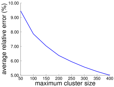
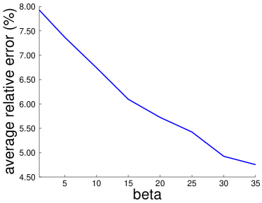
Figure 1: Average relative error vs maximum cluster size and scale factor $\beta$.

Table 2: Average adjusted Rand index values for randomly generated datasets. Best ones are marked as bold face.

	Poisson ($k$)	Poisson ($2k$)	multinomial ($k$)	multinomial ($2k$)	Gaussian ($k$)	Gaussian ($2k$)
single linkage	0.091 (0.088)	0.015 (0.030)	0.000 (0.000)	0.000 (0.000)	0.270 (0.280)	0.057 (0.055)
complete linakge	0.381 (0.091)	0.263 (0.059)	0.266 (0.144)	0.090 (0.025)	0.565 (0.166)	0.475 (0.141)
Ward’s method	0.465 (0.119)	0.273 (0.049)	0.770 (0.067)	0.564 (0.055)	0.779 (0.145)	0.763 (0.122)
RBHC-greedy	0.469 (0.112)	0.290 (0.056)	0.870 (0.046)	0.733 (0.028)	0.875 (0.087)	0.883 (0.067)
RBHC-nnca	0.469 (0.112)	0.290 (0.056)	0.865 (0.045)	0.736 (0.040)	0.875 (0.087)	0.883 (0.067)
BHC	0.265 (0.080)	0.134 (0.052)	0.907 (0.069)	0.894 (0.044)	0.863 (0.109)	0.860 (0.108)

4 EXPERIMENTS

4.1 Experiments on Synthetic Data

Testing the reducibility of $\mathsf{d}_{\star}(\cdot,\cdot)$: We tested the reducibility of $\mathsf{d}_{\star}(\cdot,\cdot)$ empirically. We repeatedly generated the three clusters $c_{0},c_{1}$ and $c_{2}$ from the exponential family distributions, and counted the number of cases where the dissimilarities between those clusters are not reducible. We also measured the average value of the relative error to support our arguments in Section 3.2. We tested three distributions; Poisson, multinomial and Gaussian. At each iteration, we first sampled the size of the clusters $|c_{0}|$, $|c_{1}|$ and $|c_{2}|$ from $\mathrm{Unif}([20,100])$. Then we sampled the three clusters from one of the three distributions, and computed $\mathsf{d}_{\star}(c_{0},c_{1}),\mathsf{d}_{\star}(c_{1},c_{2})$ and $\mathsf{d}_{\star}(c_{0},c_{2})$. We then first checked whether these three values satisfy the reducibility condition (2.2) (for example, if $\mathsf{d}_{\star}(c_{0},c_{2})$ is the smallest, we checked if $\mathsf{d}_{\star}(c_{0}\cup c_{2},c_{1})\geq\min\{\mathsf{d}_{\star}(c_{0},c_{1}),\mathsf{d}_{\star}(c_{2},c_{1})\}$). Then, for $\mathsf{d}_{\star}(c_{0},c_{1})$, we computed the approximate value $\widetilde{\mathsf{d}}_{\star}(c_{0},c_{1})$ and measured the relative error

$$2\times\left|\frac{\mathsf{d}_{\star}(c_{0},c_{1})-\widetilde{\mathsf{d}}_{\star}(c_{0},c_{1})}{\mathsf{d}_{\star}(c_{0},c_{1})+\widetilde{\mathsf{d}}_{\star}(c_{0},c_{1})}\right|.$$ (47)

We repeated this process for $100,000$ times for the three distributions and measured the average values. For Poisson distribution, we sampled the mean $\rho\sim\mathrm{Gamma}(2,0.05)$ and sampled the data from $\mathrm{Poisson}(\rho)$. We smoothed the function $\varphi(\boldsymbol{x})=\boldsymbol{x}\log(\boldsymbol{x})-\boldsymbol{x}$ as $\varphi(\boldsymbol{x}+0.01)$ to prevent degenerate function values. For multinomial distribution, we tested the case where the dimension $d$ is $10$ and the number of trials $m$ is 5. We sampled the parameter $\boldsymbol{q}\sim\mathrm{Dir}(5\cdot\mathbf{1}_{d})$ where $\mathbf{1}_{d}$ is $d$-dimensional one vector, and sampled the data from $\mathrm{Mult}(\boldsymbol{q})$. We smoothed the function $\varphi(\boldsymbol{x})=\sum_{j=1}^{d}x_{j}\log(x_{j}/m)$ as $\varphi(0.9\boldsymbol{x}+0.1m\mathbf{1}_{d}/d)$. For Gaussian, we tested with $d=10$, and sampled the mean and covariance $\boldsymbol{\mu},\boldsymbol{\Sigma}\sim{\mathcal{N}}(0,(0.08\cdot\boldsymbol{\Lambda})^{-1}){\mathcal{W}}(d+2,\boldsymbol{\Psi})$ ($\boldsymbol{\Psi}=\boldsymbol{A}\boldsymbol{A}^{\top}+d\boldsymbol{I}$ where $\boldsymbol{A}$ was sampled from unit Gaussian). We smoothed the function $\varphi(\boldsymbol{x},\boldsymbol{X})=-\frac{1}{2}\log\det(\boldsymbol{X}-\boldsymbol{x}\boldsymbol{x}^{\top})$ as $-\frac{1}{2}\log\det(\boldsymbol{X}-\boldsymbol{x}\boldsymbol{x}^{\top}+0.01\boldsymbol{I})$.

The result is summarized in Table 1. the generated dissimilarities were reducible in most case, as expected. The relative error was small, which supports our arguments of the reason why $\mathsf{d}_{\star}(\cdot,\cdot)$ is reducible with high probability. We also measured the change of average relative error by controlling two factors; the maximum cluster size $n_{\mathrm{max}}$ and variance scale factor $\beta$. We plotted the average relative error of Gaussian distribution by changing those two factors, and the relative error decreased as predicted (Figure 1).

Clustering synthetic data: We evaluated the clustering accuracies of original BHC (BHC), BHC in small-variance limit with greedy algorithm (RBHC-greedy), BHC in small-variance limit with nearest neighbor chain method (RBHC-nnca), single linkage, complete linkage, and Ward’s method. We generated the datasets from Poisson, multinomial and Gaussian distribution. We tested two types of data; 1,000 elements with 6 clusters and 2,000 elements with 12 clusters. For Poisson distribution, each mixture component was generated from $\mathrm{Poisson}(\rho)$ with $\rho\sim\mathrm{Gamma}(2,0.05)$ for both datasets. For multinomial distribution, we set $d=20$ and $m=10$ for 1,000 elements dataset, and set $d=40$ and $m=10$ for 2,000 elements datasets. For both dataset, we sampled the parameter $\boldsymbol{q}\sim\mathrm{Dir}(0.5\cdot\mathbf{1}_{d})$. For Gaussian case, we set $d=3$ for 1,000 elements dataset and set $d=6$ for 2,000 elements dataset. We sampled the parameters from ${\mathcal{N}}(0,(0.08\cdot\Lambda)^{-1}){\mathcal{W}}(\boldsymbol{\Psi},6)$ for 1,000 elements, and from ${\mathcal{N}}(0,(0.2\cdot\Lambda)^{-1}){\mathcal{W}}(\boldsymbol{\Psi},9)$ for 2,000 elements. For each distribution and type (1,000 or 2,000), we generated 10 datasets for each type and measured the average clustering accuracies.

We evaluated the clustering accuracy using the adjusted Rand index (Hubert and Arabie, 1985). For traditional agglomerative clustering algorithms, we assumed that we know the true number of clusters $k$ and cut the tree at corresponding level. For RBHC-greedy and RBHC-nnca, we selected the threshold $\lambda$ with the heuristics described in Section 3.1. For original BHC, we have to carefully tune the hyperparemters, and the accuracy was very sensitive to this setting. In the case of Poisson distribution where $\rho\sim\mathrm{Gamma}(a,b)$, we have to tune two hyperparameters $\{a,b\}$. For multinomial case where $\boldsymbol{q}\sim\mathrm{Dir}(\boldsymbol{\alpha})$, we set $\boldsymbol{\alpha}=\alpha\mathbf{1}_{d}$ and tuned $\alpha$. For Gaussian case where $(\boldsymbol{\mu},\boldsymbol{\Sigma})\sim{\mathcal{N}}(\boldsymbol{m},(r\boldsymbol{\Lambda})^{-1}){\mathcal{W}}(\nu,\boldsymbol{\Psi}^{-1})$, we have four hyperparameters $\{\boldsymbol{m},r,\nu,\boldsymbol{\Psi}\}$. We set $\boldsymbol{m}$ to be the empirical mean of $\boldsymbol{X}$ and fixed $r=0.1$ and $\nu=d+6$. We set $\boldsymbol{\Psi}=k\boldsymbol{S}$ where $\boldsymbol{S}$ is the empirical covariance of $\boldsymbol{X}$ and controlled $k$ according to the dimension and the size of the data. The result is summarized in Table 2.

The accuracies of RBHC-greedy and RBHC-nnca were best for most of the cases, and the accuracies of the two methods were almost identical expect for the multinomial distribution. BHC was best for the multinomial case where the hyperparameter tuning was relatively easy, but showed poor performance in Poisson case (we failed to find the best hyperparameter setting in that case). Hence, it would be a good choice to use RBHC-greedy or RBHC-nnca which do not need careful hyperparameter tuning, and RBHC-nnca may be the best choice considering its space and time complexity compared to RBHC-greedy.

4.2 Experiments on Real Data

We tested the agglomerative clustering algorithms on two types of real-world data. The first one was a subset of MNIST digit database (LeCun et al., 1998). We scaled down the original $28\times 28$ to $7\times 7$ and vectorized each image to be $\mathbb{R}^{49}$ vector. Then we sampled 3,000 images from the classes $0,3,7$ and $9$. We clustered this dataset with Gaussian asssumption. The second one was visual-word data extracted from Caltech101 database (Fei-Fei et al., 2004). We sampled 2,033 images from ”Airplane”, ”Mortorbikes” and ”Faces-easy” classes, and extracted SIFT features for image patches. Then we quantized those features into 1,000 visual words. We clustered the data with multinomial assumption. Table 3 shows the ARI values of agglomerative clustering algorithms. As in the synthetic experiments, the accuracy RBHC-greedy and RBHC-nnca were identical, and outperformed the traditional agglomerative clustering algorithms. BHC was best for Caltech101, where the multinomial distribution with easy hyperparameter tuning was assumed. However, BHC was even worse than Ward’s method for MNIST case, where we failed to tune $49\times 49$ matrix $\boldsymbol{\Psi}$.

Table 3: Average adjusted Rand index values for MNIST and Caltech101 datasets. Best ones are marked as bold face.

	MNIST	Caltech101
single linkage	0.000	0.000
complete linakge	0.187	0.000
Ward’s method	0.485	0.465
RBHC-greedy	0.637	0.560
RBHC-nnca	0.637	0.560
BHC	0.253	0.646

5 CONCLUSIONS

In this paper we have presented a non-probabilistic counterpart of BHC, referred to as RBHC, using a small variance relaxation when underlying likelihoods are assumed to be conjugate exponential families. In contrast to the original BHC, RBHC does not requires careful tuning of hyperparameters. We have also shown that the dissimilarity measure emerged in RBHC is reducible with high probability, so that the nearest neighbor chain algorithm was used to speed up the RBHC and to reduce the space complexity, leading to RBHC-nnca. Experiments on both synthetic and real-world datasets demonstrated the validity of RBHC.

Acknowledgements: This work was supported by National Research Foundation (NRF) of Korea (NRF-2013R1A2A2A01067464) and the IT R&D Program of MSIP/IITP (14-824-09-014, Machine Learning Center).

Appendix A Detailed Derivation in Section 3.2

For $\boldsymbol{X}_{c}=\{\boldsymbol{x}_{i}\}_{i\in c}\stackrel{{\scriptstyle\mathrm{iid}}}{{\sim}}p(\boldsymbol{x}|\beta,\boldsymbol{\theta})$, we have

$$p(\bar{t}_{c}|\beta,\boldsymbol{\theta})=\exp\bigg{\{}\beta|c|\langle\bar{t}_{c},\boldsymbol{\theta}\rangle-\beta|c|\psi(\boldsymbol{\theta})-\sum_{i\in c}h_{\beta}(\boldsymbol{x}_{i})\bigg{\}}.$$ (48)

For notational simplicity, we let $\bar{t}_{c}=\boldsymbol{y}$ from now. By the normalization property,

$$\beta|c|\psi(\boldsymbol{\theta})=\log\int\exp\bigg{\{}\beta|c|\langle\boldsymbol{y},\boldsymbol{\theta}\rangle-\sum_{i\in c}h_{\beta}(\boldsymbol{x}_{i})\bigg{\}}d\boldsymbol{y}.$$ (49)

Differentiating both sides by $\boldsymbol{\theta}$ yields

$$\beta|c|\frac{d\psi(\boldsymbol{\theta})}{d\boldsymbol{\theta}}=\int\beta|c|\boldsymbol{y}\cdot p(\boldsymbol{y}|\beta,\boldsymbol{\theta})d\boldsymbol{y},\quad\frac{d\psi(\boldsymbol{\theta})}{d\boldsymbol{\theta}}=\mathbb{E}[\boldsymbol{y}].$$ (50)

Also, we have

$$\beta|c|\frac{\partial^{2}\psi(\boldsymbol{\theta})}{\partial\theta_{j}\partial\theta_{k}} = \int\beta|c|y_{j}p(\boldsymbol{y}|\beta,\boldsymbol{\theta})\bigg{(}\beta|c|y_{j}-\beta|c|\frac{\partial\psi(\boldsymbol{\theta})}{\partial\theta_{k}}\bigg{)}dy_{j}$$ (51)

$$= \beta^{2}|c|^{2}\mathbb{E}[y_{j}y_{k}]-\beta^{2}|c|^{2}\mathbb{E}[\boldsymbol{y}]_{j}\mathbb{E}[\boldsymbol{y}]_{k}=\beta^{2}|c|^{2}\mathrm{cov}(y_{j},y_{k}).$$

Hence,

$$\frac{1}{\beta|c|}\frac{\partial^{2}\psi(\boldsymbol{\theta})}{\partial\theta_{j}\partial\theta_{k}}=\mathrm{cov}(y_{j},y_{k})=\int(y_{j}-\mathbb{E}[\boldsymbol{y}]_{j})(y_{k}-\mathbb{E}[\boldsymbol{y}]_{k})p(\boldsymbol{y}|\beta,\boldsymbol{\theta})dy_{j}dy_{k}.$$ (52)

Differentiating this again yields

$$\frac{1}{\beta|c|}\frac{\partial^{3}\psi(\boldsymbol{\theta})}{\partial\theta_{j}\partial\theta_{k}\partial\theta_{l}} = \int(y_{j}-\mathbb{E}[\boldsymbol{y}]_{j})(y_{k}-\mathbb{E}[\boldsymbol{y}]_{k})(y_{l}-\mathbb{E}[\boldsymbol{y}]_{l})p(\boldsymbol{y}|\beta,\boldsymbol{\theta})dy_{j}dy_{k}dy_{l}$$ (53)

$$= \mathbb{E}[(y_{j}-\mathbb{E}[\boldsymbol{y}]_{j})(y_{k}-\mathbb{E}[\boldsymbol{y}]_{k})(y_{l}-\mathbb{E}[\boldsymbol{y}]_{l})].$$

Unfortunately, this relationship does not continue after the third order; the fourth derivative of $\psi(\boldsymbol{\theta})$ is not exactly match to the fourth order central moment of $\boldsymbol{y}$. However, one can easily maintain the $m$th order central moment by manipulating the $m$th order derivative of $\psi(\boldsymbol{\theta})$, and $m$th order central moment always have the constant term $(\beta|c|)^{-m}$.

Equation (40) of the paper is a simple consequence of the equation (53). To prove the equation (41) of the paper, we use the following relationship:

$$\mathbb{E}\bigg{[}\frac{\epsilon_{\varphi}(\bar{\boldsymbol{x}}_{c})}{\Delta_{\varphi}(\bar{\boldsymbol{x}}_{c})}\bigg{]}\approx\frac{\mathbb{E}[\epsilon_{\varphi}(\bar{\boldsymbol{x}}_{c})]}{\mathbb{E}[\Delta_{\varphi}(\bar{\boldsymbol{x}}_{c})]}-\frac{\mathrm{cov}(\epsilon_{\varphi}(\bar{\boldsymbol{x}}_{c}),\Delta_{\varphi}(\bar{\boldsymbol{x}}_{c}))}{\mathbb{E}[\Delta_{\varphi}(\bar{\boldsymbol{x}}_{c})]^{2}}+\frac{\mathbb{E}[\epsilon_{\varphi}(\bar{\boldsymbol{x}}_{c})]\mathrm{var}[\Delta_{\varphi}(\bar{\boldsymbol{x}}_{c})]}{\mathbb{E}[\Delta_{\varphi}(\bar{\boldsymbol{x}}_{c})]^{3}}.$$ (54)

Now it is easy to show that this equation converges to zero when $\beta\to 0$; all the expectations and variances can be obtained by differentiating $\psi(\boldsymbol{\theta})$ for as many times as needed.

References

• Antoniak (1974) C. E. Antoniak. Mixtures of Dirichlet processes with applications to Bayesian nonparametric problems. The Annals of Statistics, 2(6):1152–1174, 1974.
• Banerjee et al. (2005) A. Banerjee, S. Merugu, I. S. Dhillon, and J. Ghosh. Clustering with Bregman divergences. Journal of Machine Learning Research, 6:1705–1749, 2005.
• Bregman (1967) L. M. Bregman. The relaxation method of finding the common points of convex sets and its application to the solution of problems in convex programming. USSR Computational Mathematics and Mathematical Physics, 7:200–217, 1967.
• Bruynooghe (1978) M. Bruynooghe. Classification ascendante hiérarchique, des grands ensembles de données: un algorithme rapide fondé sur la construction des voisinages réductibles. Les Cahiers de l’Analyse de Données, 3:7–33, 1978.
• Day and Edelsbrunner (1984) W. H. E. Day and H. Edelsbrunner. Efficient algorithms for agglomerative hierarchical clustering methods. Journal of Classification, 1:7–24, 1984.
• Duda et al. (2001) R. O. Duda, P. E. Hart, and D. G. Stork. Pattern Classification. John Wiely & Sons, 2001.
• Fei-Fei et al. (2004) L. Fei-Fei, R. Fergus, and P. Perona. Learning generative visual models from few training examples: An incremental Bayesian approach tested on 101 object categories. In Proceedings of the IEEE CVPR-2004 Workshop on Generative-Model Based Vision, 2004.
• Ferguson (1973) T. S. Ferguson. A Bayesian analysis of some nonparametric problems. The Annals of Statistics, 1(2):209–230, 1973.
• Heller and Ghahrahmani (2005) K. A. Heller and Z. Ghahrahmani. Bayesian hierarchical clustering. In Proceedings of the International Conference on Machine Learning (ICML), Bonn, Germany, 2005.
• Hubert and Arabie (1985) L. Hubert and P. Arabie. Comparing partitions. Journal of Classification, 2:193–218, 1985.
• Jiang et al. (2012) K. Jiang, B. Kulis, and M. I. Jordan. Small-variance asymptotics for exponential family Dirichlet process mixture models. In Advances in Neural Information Processing Systems (NIPS), volume 25, 2012.
• Kulis and Jordan (2012) B. Kulis and M. I. Jordan. Revisiting $k$-means: New algorithms via Bayesian nonparametrics. In Proceedings of the International Conference on Machine Learning (ICML), Edinburgh, Scotland, UK, 2012.
• Lance and Williams (1967) G. N. Lance and W. T. Williams. A general theory of classicificatory sorting strategies: 1 hierarchical systems. The Computing Journal, 9:373–380, 1967.
• LeCun et al. (1998) Y. LeCun, L. Bottou, Y. Bengio, and P. Haffner. Gradient-based learning applied to document recognition. Proceedings of the IEEE, 86(11):2278–2324, 1998.
• Lee and Choi (2014) J. Lee and S. Choi. Incremental tree-based inference with dependent normalized random measures. In Proceedings of the International Conference on Artificial Intelligence and Statistics (AISTATS), Reykjavik, Iceland, 2014.
• Telgarsky and Dasgupta (2012) M. Telgarsky and S. Dasgupta. Agglomerative Bregman clustering. In Proceedings of the International Conference on Machine Learning (ICML), Edinburgh, Scotland, UK, 2012.
• Wallach et al. (2010) H. M. Wallach, S. T. Jensen, L. Dicker, and K. A. Heller. An alternative prior process for nonparametric Bayesian clustering. In Proceedings of the International Conference on Artificial Intelligence and Statistics (AISTATS), Sardinia, Italy, 2010.
• Ward (1963) J. H. Ward. Hierarchical grouping to optimize an objective function. Journal of the American Statistical Association, pages 236–244, 1963.