Nonequilibrium transport through quantum-wire junctions and boundary defects for free massless bosonic fields

Abstract

We consider a model of quantum-wire junctions where the latter are described by conformal-invariant boundary conditions of the simplest type in the multicomponent compactified massless scalar free field theory representing the bosonized Luttinger liquids in the bulk of wires. The boundary conditions result in the scattering of charges across the junction with nontrivial reflection and transmission amplitudes. The equilibrium state of such a system, corresponding to inverse temperature $\beta$ and electric potential $V$, is explicitly constructed both for finite and for semi-infinite wires. In the latter case, a stationary nonequilibrium state describing the wires kept at different temperatures and potentials may be also constructed following Ref. [32]. The main result of the present paper is the calculation of the full counting statistics (FCS) of the charge and energy transfers through the junction in a nonequilibrium situation. Explicit expressions are worked out for the generating function of FCS and its large-deviations asymptotics. For the purely transmitting case they coincide with those obtained in Refs. [10, 11], but numerous cases of junctions with transmission and reflection are also covered. The large deviations rate function of FCS for charge and energy transfers is shown to satisfy the fluctuation relations of Refs. [2, 12]. The expressions for FCS obtained here are compared with the Levitov-Lesovic formulae of Refs. [29, 28].

1 Introduction

The transport phenomena in quantum wires (carbon nanotubes, semiconducting, metallic and molecular nanowires, quantum Hall edges) and, in particular, across their junctions, have attracted a lot of interest in recent times,  see e.g.  [16, 14]. To a good approximation, the charge carriers inside the wires may be described by the Tomonaga-Luttinger model [46, 42, 22, 26]. In the low energy limit, such a model reduces to a relativistic 1+1 dimensional interacting fermionic field theory that can also be represented by free massless bosonic fields. The junction between the leads couples together the conformal field theories (CFTs) describing at low energies the bulk volumes of the wires. Specific features of the coupling depend on how the junction is realized. Various models that couple two or more wires locally at their connected extremities were considered in the literature,  see e.g. [20, 36, 34, 35] where important results about transport properties of such models of wire-junctions were obtained. The low-energy long-distance effect of the interaction at the junction may be described with the use of boundary CFT, similarly as the effect of a magnetic impurity in the multi-channel Kondo problem [1]. Even if the coupling of the Luttinger liquid theories introduced by the junction breaks the conformal symmetry, the latter should be restored in the long-distance scaling limit. In the scaling limit, the effect of the junction will be represented, using the “folding trick” of ref. [49], by a conformal boundary defect in the tensor product of the bulk CFTs of individual wires [7]. Such a boundary defect preserves half of the conformal symmetry of the bulk theory. Examples of conformal boundary defects that describe the renormalization group fixed points of Luttinger liquid theories with a coupling localized at the junction were discussed in [20, 36, 34, 35]. It was also realized that the boundary CFT description of the junction of wires gives via the Green-Kubo formalism a direct access to the low temperature electric conductance of junctions [35, 39, 40] that measure small currents induced by placing different wires in slightly different external electric potentials. Getting hold of the transport properties of the quantum-wire junctions beyond the linear response regime is more complicated, see [20] for an early result using an exact integrability of a model of contact between two wires. The CFT approach seems also helpful here. It was shown in [10, 11, 12, 19] that for some boundary defects (those with pure transmission of charge or energy), not only the electric and thermal conductance but also the long-time asymptotics of the full counting statistics (FCS) of charge and energy transfers through the junction may be calculated for the wires initially equilibrated at different temperatures and different potentials. Moreover, steady nonequilibrium states obtained at long times from such initial conditions could be explicitly constructed. Physical restrictions for the applicability of the CFT approach in such a nonequilibrium situations were also discussed in some detail in those works, in particular in [11], see also [8, 18, 4, 15]. The incorporation of junctions corresponding to boundary defects with transmission and reflection into that approach poses more problems, although for a junction of two CFTs a general scheme has been recently laid down in [13], together with some examples.

The present paper arose from an attempt to calculate the FCS for nonequilibrium charge and energy transfers for simple conformal boundary defects with transmission and reflection. We describe each of $\,N\,$ wires by a compactified free massless $1+1$-dimensional bosonic field, with the compactification radius related to the Luttinger model coupling constants that may be different for different wires. The product theory is a toroidal compactification of the massless $N$-component free field,  i.e.,  on the classical level, its field takes values in the torus $\,U(1)^{N}$.  In such a theory, we consider the simplest conformal boundary defects that restrict the boundary values of the field at the junction to a subgroup $\,{\cal B}\subset U(1)^{N}\,$ isomorphic to the torus $\,U(1)^{M}\,$ with $M\leq N$. In the string-theory jargon, $\,{\cal B}\,$ is called the D(irichlet)-brane [38]. First, we study the wires of finite length $\,L\,$ with the reflecting boundary condition at their ends not connected to the junction. The overall $U(1)$-symmetry of the theory is imposed, leading to the conservation of the total electric charge. We show that the boundary defect gives rise to an $N\times N$ scattering matrix $\,S\,$ that relates linearly the left-moving and the right-moving components of the electric currents in various wires. The classical theory described above may be canonically quantized preserving the latter property. The exact solution for the quantum theory includes the formula for the partition function of the equilibrium state corresponding to inverse temperature $\beta$ and electric potential $V$ and for the equilibrium correlation functions of the chiral components of the electric currents. The thermodynamic limit $\,L\to\infty\,$ may then be performed giving rise to a free-field theory that was constructed directly for $\,L=\infty\,$ in [32]. In that limit, the equilibrium correlation functions involving only left-moving (or only right-moving) currents factorize into the product of contributions from the individual wires. This property was used in [32],  following the earlier work [31], to construct a nonequilibrium stationary state (NESS) where the correlation functions of left-moving currents factorize into the product of equilibrium contributions from individual wires, each corresponding to a different temperature and a different potential. The NESS correlation functions involving also the right-moving currents are reduced to those of the left-moving ones using the scattering relation between the chiral current components. Following the approach of [10, 11], we show that such a state is obtained if one prepares disconnected wires each in the equilibrium state at different temperature and potential and then one connects the wires instantaneously and lets the initial state evolve for a long time [41].

The main aim of the present paper is the study of the FCS for charge and energy (heat) transfers through the junction modeled by the brane defect of the type described above. Similarly as in [11], the FCS is obtained from a two-time measurement protocol. First, the total charge and total energy is measured in each of the disconnected wires of finite length $\,L\,$ prepared in equilibria with different temperatures and potentials. Next the wires are instantaneously connected and evolve for time $\,t\,$ with the dynamics described by the field theory with the brane defect. After time $\,t$,  the wires are disconnected again and the second measurement of total charge and total energy in individual wires is performed. The FCS is encoded in the characteristic function of the probability distribution of the changes of total charge and total energy of individual wires. The above protocol is not practical for long wires as the total charge and and total energy of the wires, unlike their change in time, behave extensively with $\,L$,  but a similar charge and energy transfer statistics should be obtainable from an indirect measurement protocol where one observes the evolution of gauges coupled appropriately to the wires and registering the flow of charge and energy through the junction, see [29, 30]. In our model, we compute the generating function of FCS of charge transfers explicitly for any $\,L\,$ and $\,t\,$ and confirm that it takes for large $\,t\,$ the large-deviations exponential form that is independent of whether $\,L\,$ is sent to infinity first or,  e.g.,  kept equal to $\,t/2$.  The equality of the large deviation forms for the two limiting procedures appears, however, to be less obvious than one could have expected. The choice $\,L=t/2\,$ leads to the simplest calculation of the large deviation rate function and was implicitly employed in [10, 11], where it was argued that it reproduces correctly the large deviations of the FCS for the junction of semi-infinite wires. We also compute explicitly the generating function of the FCS for heat transfers for $\,L=t/2\,$ and its large deviations form. The case of general $\,L\,$ and $\,t\,$ could be also dealt with but the corresponding formulae are considerably heavier and we did not present them here. The generating function of the joint FCS of the charge and energy transfers for $\,L=t/2\,$ and its large deviations form were also obtained. To our knowledge, the calculations of FCS presented in this paper are the first ones obtained for junctions with transmission and reflection modeled by conformal boundary defects. It should be mentioned, however, that in a different physical setup, the FCS of charge transfers across an inhomogeneous Luttinger liquid conductor connected to two leads with distinct energy distributions was obtained by a “nonequilibrium bosonization” in [24, 25, 33].

The present paper is organized as follows. In Sec. 2, we briefly recall the description of relativistic free massless fermions and bosons on an interval. We discuss the correspondence between the two theories and how it extends to the case of the Luttinger model of interacting fermions. Sec. 3 describes in detail the model of a junction based on a toroidal compactification of the multi-component massless bosonic free field with a boundary defect of the type mentioned above. We discuss first the classical theory on a space-interval of length $\,L\,$ and subsequently canonically quantize that theory in Sec. 4. In particular, we show how the scattering matrix $\,S\,$ relating the chiral components of the electric current arises from the brane describing the boundary defect. Sec. 5 constructs the equilibrium states of the quantized theory labeled by inverse temperature $\,\beta\,$ and electric potential $\,V$. In Sec. 6, we discuss the Euclidean functional integral representation of the equilibrium state and in Sec. 7, its dual closed-string representation resulting from the interchange of time and space in the functional integral. The closed-string picture is particularly convenient in the thermodynamic limit $\,L\to\infty\,$ of the equilibrium state that is analyzed in Sec. 8.  Sec. 9 discusses the NESS of the junction of semi-infinite wires kept in different temperatures and different electric potentials. By considering the nonequilibrium state for close temperatures and potentials, we obtain as a byproduct the formulae for the electric and thermal conductance of the junction. The central Sec. 10 is devoted to the analysis of FCS for charge and heat transfers through the junction. Subsecs. 10.1 and 10.2 treat the charge transport, Subsec. 10.3 that of heat, and Subsec. 10.4 the joint FCS for both. Sec. 11 compares the generating function of FCS for charge and heat transfers obtained in this paper with those given by the Levitov-Lesovik formulae for free fermions [29, 30] and free bosons [28]. In Sec. 12, we specify our general formulae to few simplest cases of junctions of two and three wires. Finally, Sec. 13 collects our conclusions and discusses the possible generalizations and open problems. Appendix A contains the calculations of the generating functional of FCS for charge transfers at general $\,t\,$ and $\,L$.  Appendix B performs the computation of certain bosonic Fock space expectations that are needed to obtain the generating function of FCS for heat transfers through the junction. Appendix C calculates the quadratic contribution to the Levitov-Lesovik large-deviations rate function of charge transfers for free fermions.

Acknowledgements: The authors thank D. Bernard for discussions on nonequilibrium CFT and J. Germoni for Ref. [44]. A part of the work of K.G. was done within the STOSYMAP project ANR-11-BS01-015-02.

2 Field theory description of quantum wires

2.1 Classical fermions

Consider a fermionic 1+1-dimensional field theory describing noninteracting conduction electrons in a quantum wire of length $\,L$. To a good approximation such electrons have a linear dispersion relation around the Fermi surface. For simplicity, we shall ignore here the electron spin. The classical action functional of the anticommuting Fermi fields of such a theory has the form

$$S[\bar{\psi},\psi]\,=\,\frac{{}_{2{\rm i}}}{{}^{\pi}}\int{\rm d}t\int\limits_{0}^{L}\big{[}\bar{\psi}^{\ell}\partial_{-}\psi^{\ell}\,+\,\bar{\psi}^{r}\partial_{+}\psi^{r}\big{]}{\rm d}x\,,$$ (2.1)

where $\,\partial_{\pm}=\frac{1}{2}(\partial_{t}\pm\partial_{x})$,  with the boundary conditions

$$\psi^{\ell}(t,0)=\psi^{r}(t,0)\,,\qquad\psi^{\ell}(t,L)=-\psi^{r}(t,L)\,.$$ (2.2)

We use the Fermi velocity $\,v_{F}\,$ to express time in the same units as length. The classical equations obtained by extremizing action (2.1) are

$$\partial_{-}\psi^{\ell}=0=\partial_{-}\bar{\psi}^{\ell}\,,\qquad\partial_{+}\psi^{r}=0=\partial_{+}\bar{\psi}^{r}$$ (2.3)

and their solutions take the form:

$$\psi^{\ell}(t,x)\,=\,\sqrt{\frac{{}_{\pi}}{{}^{2L}}}\,\sum\limits_{p\in{\mathbb{Z}}+\frac{{}_{1}}{{}^{2}}}c_{p}\,{\rm e}^{-\frac{\pi{\rm i}p(t+x)}{L}}\,=\,\psi^{r}(t,-x)\,,$$ (2.4)

$$\bar{\psi}^{\ell}(t,x)\,=\,\sqrt{\frac{{}_{\pi}}{{}^{2L}}}\,\sum\limits_{p\in{\mathbb{Z}}+\frac{{}_{1}}{{}^{2}}}\bar{c}_{-p}\,{\rm e}^{-\frac{\pi{\rm i}p(t+x)}{L}}\,=\,\bar{\psi}^{r}(t,-x)\,.$$ (2.5)

The space of classical solutions comes equipped with the odd symplectic form

$$\Omega\,=\,\frac{{}_{{\rm i}}}{{}^{\pi}}\int\limits_{0}^{L}\big{[}\delta\bar{\psi}^{\ell}\wedge\delta\psi^{\ell}+\delta\bar{\psi}^{r}\wedge\delta\psi^{r}\big{]}\,{\rm d}x\,=\,{\rm i}\sum\limits_{p\in{\mathbb{Z}}+\frac{{}_{1}}{{}^{2}}}\delta\bar{c}_{p}\wedge\delta c_{p}$$ (2.6)

leading to the odd Poisson brackets

$$\{c_{p},c_{p^{\prime}}\}\,=\,0\,=\,\{\bar{c}_{p},\bar{c}_{p^{\prime}}\}\,,\qquad\{c_{p},\bar{c}_{p^{\prime}}\}\,=\,-{\rm i}\,\delta_{p,p^{\prime}}\,.$$ (2.7)

The $U(1)$ symmetry

$$\psi^{\ell,r}\ \mapsto\ {\rm e}^{-{\rm i}\alpha}\psi^{\ell,r}\,,\qquad\bar{\psi}^{\ell,r}\ \mapsto\ {\rm e}^{{\rm i}\alpha}\bar{\psi}^{\ell,r}$$ (2.8)

corresponds to the Noether current

$$J^{0}=\frac{{}_{1}}{{}^{\pi}}(\bar{\psi}^{\ell}\psi^{\ell}+\bar{\psi}^{r}\psi^{r})\,,\qquad J^{1}=\frac{{}_{1}}{{}^{\pi}}(\bar{\psi}^{r}\psi^{r}-\bar{\psi}^{\ell}\psi^{\ell})$$ (2.9)

with the chiral components

$$J^{\ell}=\frac{{}_{1}}{{}^{2}}(J^{0}-J^{1})=\frac{{}_{1}}{{}^{\pi}}\bar{\psi}^{\ell}\psi^{\ell}\,,\qquad J^{r}=\frac{{}_{1}}{{}^{2}}(J^{0}+J^{1})=\frac{{}_{1}}{{}^{\pi}}\bar{\psi}^{r}\psi^{r}$$ (2.10)

and the conserved charge

$$Q=\int\limits_{0}^{L}J^{0}(t,x)\,{\rm d}x=\sum\limits_{p\in\frac{1}{2}+\mathbb{Z}}c_{p}^{\dagger}c_{p}\,.$$ (2.11)

The classical Hamiltonian is

$$H\,=\,\frac{{}_{i}}{{}^{\pi}}\int\limits_{0}^{L}\big{[}\bar{\psi}^{\ell}\partial_{x}\psi^{\ell}-\bar{\psi}^{r}\partial_{x}\psi^{r}\big{]}\,{\rm d}x\,=\,\frac{{}_{\pi}}{{}^{L}}\sum\limits_{p\in{\mathbb{Z}}+\frac{{}_{1}}{{}^{2}}}k\,\bar{c}_{p}c_{p}\,.$$ (2.12)

2.2 Quantum fermions

Quantized Fermi fields $\psi^{\ell}$ and $\psi^{r}$ are given by expressions (2.4) with operators $\,c_{p}\,$ and their adjoints $c_{p}^{\dagger}$ satisfying the canonical anticommutation relations

$$[c_{p},c_{p^{\prime}}]_{{}_{+}}\,=\,0\,=\,[c_{p}^{\dagger},c_{p^{\prime}}^{\dagger}]_{{}_{+}}\,,\qquad[c_{p},c_{p^{\prime}}^{\dagger}]_{{}_{+}}\,=\,\delta_{p,p^{\prime}}\,.$$ (2.13)

They act in the fermionic Fock space ${\mathcal{F}}_{f}$ built upon the normalized vacuum state $\,|0\rangle_{{}_{f}}\,$ annihilated by $\,c_{p}\,$ and $\,c_{-p}^{\dagger}\,$ for $\,p>0\,$ (the annihilation operators of electrons and holes, respectively).  Upon quantization, fields $\,\bar{\psi}^{\ell}\,$ and $\,\bar{\psi}^{r}\,$ become the hermitian adjoints of $\,\psi^{\ell}\,$ and $\,\psi^{r}$.  The quantum $U(1)$ currents have the chiral components

$$J^{\ell}=\frac{{}_{1}}{{}^{\pi}}:\bar{\psi}^{\ell}\psi^{\ell}:\,,\qquad J^{r}=\frac{{}_{1}}{{}^{\pi}}:\bar{\psi}^{r}\psi^{r}:$$ (2.14)

and the conserved $U(1)$ (electric) charge is

$$Q=\int\limits_{0}^{L}J^{0}\,{\rm d}x=\int\limits_{0}^{L}(J^{\ell}+J^{r})\,{\rm d}x\,=\,\sum\limits_{p\in{\mathbb{Z}}+\frac{{}_{1}}{{}^{2}}}:c_{p}^{\dagger}c_{p}:.$$ (2.15)

The fermionic Wick ordering putting (electron and hole) creation operators $\,c_{p}\,$ and $\,c_{-p}^{\dagger}\,$ for $p<0$ to the left of annihilators $\,c_{p}\,$ and $\,c_{-p}^{\dagger}\,$ for $p>0$,  with a minus sign whenever a pair is interchanged, assures that the vacuum $|0\rangle_{{}_{f}}$ has zero charge.  The quantum Hamiltonian is

$$H\,=\,\frac{{}_{\pi}}{{}^{L}}\Big{(}\sum\limits_{p\in{\mathbb{Z}}+\frac{{}_{1}}{{}^{2}}}p:c_{p}^{\dagger}c_{p}:-\,\frac{{}_{1}}{{}^{24}}\Big{)},$$ (2.16)

where the constant contribution is that of the zeta-function regularized zero-point energy

$$\sum\limits_{p<0}p=-\frac{{}_{1}}{{}^{2}}\sum\limits_{n=1}^{\infty}n+\sum\limits_{n=1}^{n}n=\frac{{}_{1}}{{}^{2}}\zeta(-1)=-\frac{{}_{1}}{{}^{24}}\,.$$ (2.17)

2.3 Classical bosons

Consider now a bosonic 1+1-dimensional massless free field $\varphi(t,x)$ defined modulo $2\pi$ on the spacetime $\mathbb{R}\times[0,L]$, with the action functional

$$S[\varphi]=\frac{{}_{r^{2}}}{{}^{4\pi}}\int{\rm d}t\int\limits_{0}^{L}\big{[}(\partial_{t}\varphi)^{2}-(\partial_{x}\varphi)^{2}\big{]}\,{\rm d}x\,.$$ (2.18)

We shall impose on $\,\varphi(t,x)\,$ the Neumann boundary conditions

$$\partial_{x}\varphi(t,0)\,=\,0\,=\,\partial_{x}\varphi(t,L)\,.$$ (2.19)

Such a scalar field will be viewed as having the range of its values compactified to the circle of radius $r$ with metric $r^{2}(d\varphi)^{2}$. The classical solutions extremizing action (2.18) have the form

$$\varphi(t,x)=\varphi^{\ell}(t,x)+\varphi^{r}(t,x)$$ (2.20)

with

$$\varphi^{\ell}(t,x)\,=\,\frac{{}_{1}}{{}^{2}}\varphi_{0}+\frac{{}_{\pi}}{{}^{2L}}\alpha_{0}(t+x)+{\rm i}\sum_{0\not=n\in{\mathbb{Z}}}\frac{{}_{1}}{{}^{2n}}\,\alpha_{2n}\,{\rm e}^{-\frac{\pi{\rm i}n(t+x)}{L}}=\varphi^{r}(t,-x)$$ (2.21)

and $\,\bar{\alpha}_{2n}=\alpha_{-2n}$.  The labeling of modes $\alpha_{2n}$ by even integers is for the later convenience. The symplectic form on the space of classical solutions is equal to

$$\Omega=\frac{{}_{r^{2}}}{{}^{2}}\delta\alpha_{0}\wedge\delta\varphi_{0}-\frac{{}_{{\rm i}\,r^{2}}}{{}^{2}}\sum_{n\neq 0}\frac{{}_{1}}{{}^{2n}}\delta\alpha_{2n}\wedge\delta\alpha_{-2n}\,,$$ (2.22)

leading to the Poisson brackets

$$\{\alpha_{0},\varphi_{0}\}\,=\,-2r^{-2}\,,\qquad\{\alpha_{2n},\alpha_{2n^{\prime}}\}\,=\,-2n{\rm i}r^{-2}\,\delta_{n+n^{\prime},0}\,.$$ (2.23)

The $U(1)$ symmetry

$$\varphi\ \mapsto\ \varphi+\alpha$$ (2.24)

corresponds to the Noether current

$$J^{0}\,=\,\frac{{}_{r^{2}}}{{}^{2\pi}}\partial_{t}\varphi\,,\qquad J^{1}\,=\,-\frac{{}_{r^{2}}}{{}^{2\pi}}\partial_{x}\varphi$$ (2.25)

with the chiral components

$$J^{\ell,r}(t,x)\,=\,\frac{{}_{r^{2}}}{{}^{2\pi}}\partial_{\pm}\varphi(t,x)\,=\,\frac{{}_{r^{2}}}{{}^{4L}}\sum\limits_{n\in{\mathbb{Z}}}\alpha_{2n}\,{\rm e}^{-\frac{\pi{\rm i}n(t\pm x)}{L}},$$ (2.26)

where the upper sign pertains to the left-moving component depending on $x^{+}=t+x$ and the lower one to the right-moving one depending on $x^{-}=t-x$.  The classical Hamiltonian takes the form

$$H\,=\,\frac{{}_{r^{2}}}{{}^{4\pi}}\int\limits_{0}^{L}\big{[}(\partial_{t}\varphi)^{2}+(\partial_{x}\varphi)^{2}\big{]}{\rm d}x\,=\,\frac{{}_{\pi r^{2}}}{{}^{4L}}\sum\limits_{n\in{\mathbb{Z}}}\alpha_{2n}\alpha_{-2n}\,.$$ (2.27)

2.4 Quantum bosons

The space $\,{\cal H}_{0}\,$ of quantum states corresponding to the zero modes $\,\varphi_{0},\alpha_{0}\,$ may be represented as $\,L^{2}(U(1))$,  with $\,\varphi_{0}\,$ viewed as the angle in $\,U(1)$. $\,\alpha_{0}\,$ acts then as $\,-2{\rm i}r^{-2}\frac{\partial}{\partial\varphi_{0}}\,$ assuring the commutation relation $\,[\alpha_{0},\varphi_{0}]=-2{\rm i}r^{-2}$.  An orthonormal basis of $\,{\cal H}_{0}\,$ is composed of the states

$$|k\rangle\,=\,{\rm e}^{{\rm i}k\varphi_{0}}$$ (2.28)

with

$$\alpha_{0}|k\rangle\,=\,2r^{-2}k\,|k\rangle\,.$$ (2.29)

The excited modes $\,\alpha_{2n}=\alpha_{-2n}^{\dagger}$ with the commutation relations

$$[\alpha_{2n},\alpha_{2n^{\prime}}]\,=\,2n\,r^{-2}\,\delta_{n+n^{\prime},0}$$ (2.30)

are represented in the bosonic Fock space $\,{\mathcal{F}}_{b}\,$ built upon the vacuum state $\,|0\rangle_{b}\,$ annihilated by $\,\alpha_{2n}\,$ with $n>0$. The total bosonic space of states is $\,{\cal H}_{b}={\cal H}_{0}\otimes{\mathcal{F}}_{b}$.  We shall identify $\,{\cal H}_{0}\,$ with its subspace $\,{\cal H}_{0}\otimes|0\rangle_{b}\,$ and the state $\,|0\rangle\in{\cal H}_{0}\,$ with the vacuum $\,|0\rangle\otimes|0\rangle_{b}$.  The chiral components $\,J^{\ell,r}\,$ of the quantum $U(1)$ current are given by the right hand side of Eq. (2.26). The conserved $U(1)$ charge takes the form

$$Q\,=\,\int\limits_{0}^{L}J^{0}\,{\rm d}x\,=\,\frac{{}_{1}}{{}^{2}}r^{2}\alpha_{0}$$ (2.31)

so that $\,Q|k\rangle=k|k\rangle\,$ and it acts trivially in $\,{\mathcal{F}}_{b}$.  The quantum Hamiltonian requires a bosonic Wick reordering putting the creators $\alpha_{-2n}$ for $n>0$ to the left of annihilators $\alpha_{2n}$ in the classical expression. Explicitly,

$$H\,=\,\frac{{}_{\pi r^{2}}}{{}^{4L}}\alpha_{0}^{2}\,+\,\frac{{}_{\pi r^{2}}}{{}^{2L}}\sum\limits_{n=1}^{\infty}\alpha_{-2n}\alpha_{2n}\,-\,\frac{{}_{\pi}}{{}^{24L}}\,,$$ (2.32)

where the constant term is the contribution of the zeta-function regularized zero-point energy

$$\frac{{}_{\pi r^{2}}}{{}^{4L}}\sum\limits_{n=1}^{\infty}2nr^{-2}\,=\,\frac{{}_{\pi}}{{}^{2L}}\zeta(-1)\,=\,-\frac{{}_{\pi}}{{}^{24L}}\,.$$ (2.33)

2.5 Boson-fermion correspondence

In one space dimension there is an equivalence between quantum relativistic free fermions and free bosons that provides a powerful tool for the analysis of such systems [43, 27], see also [45] for the historical account. In the context of the fermionic system described in Sec. 2.2, such an equivalence involves the free bosonic field of Sec. 2.4 with the compactification radius $\,r=\sqrt{2}\,$ and is realized by a unitary isomorphism $\,{\cal I}:{\cal H}_{b}\rightarrow{\cal H}_{f}\,$ that maps vacuum to vacuum, $\,{\cal I}\,|0\rangle_{b}=|0\rangle_{f}$,  and intertwines the action of $U(1)$ currents and the Hamiltonians.  In particular,

$${\cal I}\,\,\alpha_{2n}\,=\,\sum\limits_{p\in\frac{1}{2}+{\mathbb{Z}}}:c_{p}^{\dagger}c_{p+n}:\,{\cal I}\,.$$ (2.34)

The Fermi fields are intertwined by $\,{\cal I}\,$ with the bosonic vertex operators:

$$\psi^{\ell}(t,x)\,{\cal I}\,=\,{\cal I}\ \sqrt{\frac{{}_{\pi}}{{}^{2L}}}:{\rm e}^{-2{\rm i}\varphi^{\ell}(t,x)}:\,\ \equiv \ \,\,{\cal I}\ \sqrt{\frac{{}_{\pi}}{{}^{2L}}}\,{\rm e}^{\frac{\pi{\rm i}}{2L}(t+x)}\,{\rm e}^{-{\rm i}\varphi_{0}}\,{\rm e}^{-\frac{\pi{\rm i}}{L}\alpha_{0}(t+x)}$$ (2.35)

$$\times\ {\rm e}^{\,\sum\limits_{n<0}\frac{1}{n}\alpha_{2n}{\rm e}^{-\frac{\pi{\rm i}n(t+x)}{L}}}\,{\rm e}^{\,\sum\limits_{n>0}\frac{1}{n}\alpha_{2n}{\rm e}^{-\frac{\pi{\rm i}n(t+x)}{L}}},$$ (2.36)

$$\bar{\psi}^{\ell}(t,x)\,{\cal I}\,=\,{\cal I}\ \sqrt{\frac{{}_{\pi}}{{}^{2L}}}:{\rm e}^{2{\rm i}\varphi^{\ell}(t,x)}:\,\ \equiv \ \,\,{\cal I}\ \sqrt{\frac{{}_{\pi}}{{}^{2L}}}\,{\rm e}^{\frac{\pi{\rm i}}{2L}(t+x)}\,{\rm e}^{i\varphi_{0}}\,{\rm e}^{\frac{\pi{\rm i}}{L}\alpha_{0}(t+x)}$$ (2.38)

$$\times\ {\rm e}^{-\sum\limits_{n<0}\frac{1}{n}\alpha_{2n}{\rm e}^{-\frac{\pi{\rm i}n(t+x)}{L}}}\,{\rm e}^{-\sum\limits_{n>0}\frac{1}{n}\alpha_{2n}{\rm e}^{-\frac{\pi{\rm i}n(t+x)}{L}}}.$$ (2.39)

2.6 Luttinger model

The interaction of electrons near the Fermi surface gives rise to the addition of a perturbation to the free field Hamiltonian (2.16) that in the leading order takes the form of a combination of quartic terms in the free fermionic fields:

$$H^{\rm int}\,=\,\frac{{}_{1}}{{}^{2\pi^{2}}}\int\limits_{0}^{L}\big{[}2g_{2}(:\bar{\psi}^{\ell}\psi^{\ell}:)(:\bar{\psi}^{r}\psi^{r}:)+g_{4}\big{(}(:\bar{\psi}^{\ell}\psi^{\ell}:)^{2}+(:\bar{\psi}^{r}\psi^{r}:)^{2}\big{)}\big{]}\,{\rm d}x\,+\,{\rm const.}\,,$$ (2.40)

where an infinite constant is needed to make the operator well defined in the fermionic Fock space. Such a perturbation defines the Luttinger model of spinless electrons in one-dimensional crystal [46]. The crucial fact that enables an exact solution of such a model is that, under the bosonization map, the above perturbation becomes quadratic in the free bosonic field:

$$H^{\rm int}\ {\cal I} =\,{\cal I}\ \frac{{}_{1}}{{}^{2\pi^{2}}}\int\limits_{0}^{L}:\big{[}2g_{2}(\partial_{+}\varphi)(\partial_{-}\varphi)\,+\,g_{4}\,((\partial_{+}\varphi)^{2}+(\partial_{-}\varphi)^{2})\big{]}:\,{\rm d}x\,+\,{\rm const.}$$ (2.41)

$$=\,{\cal I}\ \frac{{}_{1}}{{}^{4\pi^{2}}}\int\limits_{0}^{L}:\big{[}(g_{4}+g_{2})(\partial_{t}\varphi)^{2}+(g_{4}-g_{2})(\partial_{x}\varphi)^{2}\big{]}:\,{\rm d}x\,+\,{\rm const.}\,,$$ (2.42)

where on the bosonic side the Wick ordering takes care of the diverging part of the constant on the fermionic side. The perturbed bosonic Hamiltonian has then the form

$$H^{\rm tot}=H+H^{\rm int}\,=\,\frac{{}_{1}}{{}^{4\pi^{2}}}\int\limits_{0}^{L}:\big{[}(2\pi+g_{4}+g_{2})(\partial_{t}\varphi)^{2}+(2\pi+g_{4}-g_{2})(\partial_{x}\varphi)^{2}\big{]}:\,{\rm d}x\,+\,{\rm const.}$$ (2.43)

in terms of the free field $\,\varphi(t,x)\,$ with the compactification radius $\,r=\sqrt{2}$.  $H^{\rm tot}\,$ corresponds to the classical Hamiltonian

$$H^{\rm tot}\,=\,\frac{{}_{1}}{{}^{4}}\int\limits_{0}^{L}\big{[}(2\pi+g_{4}+g_{2})\Pi^{2}+\frac{{}_{2\pi+g_{4}-g_{2}}}{{}^{\pi^{2}}}(\partial_{x}\varphi)^{2}\big{]}\,{\rm d}x\,,$$ (2.44)

where $\,\Pi(t,x)=\frac{1}{\pi}(\partial_{t}\varphi)(t,x)\,$ is the field canonically conjugate to $\,\varphi(t,x)$.  The classical Lagrangian related to the above classical Hamiltonian is obtained by the Legendre transform:

$$L^{\rm tot} =\,\frac{{}_{1}}{{}^{2\pi}}\int\limits_{0}^{L}\big{[}\frac{{}_{2\pi}}{{}^{2\pi+g_{4}+g_{2}}}(\partial_{t}\varphi)^{2}-\frac{{}_{2\pi+g_{4}-g_{2}}}{{}^{2\pi}}(\partial_{x}\varphi)^{2}\big{]}\,{\rm d}x =\,\frac{{}_{r^{2}}}{{}^{4\pi}}\int\limits_{0}^{\alpha^{-1}L}\big{[}(\partial_{t}\varphi)^{2}-(\partial_{x^{\prime}}\varphi)^{2}\big{]}\,{\rm d}x^{\prime}$$ (2.45)

for $\,x=\alpha x^{\prime}$,  where

$$\frac{{}_{r^{2}}}{{}^{2}}\,\equiv\,K\,=\,\sqrt{\frac{{}_{2\pi+g_{4}-g_{2}}}{{}^{2\pi+g_{4}+g_{2}}}}\,,\qquad\alpha\,\equiv\,\frac{{}_{v_{\rm ren}}}{{}^{v_{F}}}\,=\,\frac{{}_{\sqrt{(2\pi+g_{4})^{2}-g_{2}^{2}}}}{{}^{2\pi}}\,.$$ (2.46)

Hence after the change of the spatial variable,  Lagrangian $\,L^{\rm tot}\,$ becomes that of the free bosonic field compactified on the radius $\,r\,$ that is different from $\,r=\sqrt{2}\,$ if $\,g_{2}\not=0$.  The factor $\,\alpha\,$ gives the multiplicative renormalization of the wave velocity $\,v_{F}\,$ due to the interactions (we assume that $\,|2\pi+g_{4}|>|g_{2}|$). The quantization of the free bosonic theory compactified at radius $\,r\,$ discussed in Sec. 2.4 provides the exact solution of the Luttinger model on the quantum level.

3 Bosonic model of a junction of quantum wires

In the spirit of the “folding trick” of [49, 37],  see Fig. 1,  we shall model a junction of $N$ quantum wires by a compactified free field $\,\bm{g}(t,x)\,$ with $N$-components $\,g_{i}(t,x)={\rm e}^{{\rm i}\varphi_{i}(t,x)}\in U(1)\,$ defined on the spacetime $\mathbb{R}\times[0,L]$,  with the action functional

$$S[\bm{g}]=\sum\limits_{i=1}^{N}\frac{{}_{r_{i}^{2}}}{{}^{4\pi}}\int{\rm d}t\int\limits_{0}^{L}\big{(}(\partial_{t}\varphi_{i})^{2}-(\partial_{x}\varphi_{i})^{2}\big{)}\,{\rm d}x$$ (3.1)

and appropriate boundary conditions. The compactification radii $\,r_{i}\,$ may be different for different wires, corresponding to different quartic coupling constants $g_{2i}$ and $g_{4i}$ in the Luttinger models describing the electrons in the individual wires, see Eq. (2.46) of Sec. 2.6. We shall impose the Neumann reflecting boundary conditions at the free ends of the wires:

$$\partial_{x}\bm{\varphi}(t,L)=0\,,$$ (3.2)

where $\,\bm{\varphi}\equiv(\varphi_{i})$.  Note that we use the rescaled spatial variables in the wires so that the lengths of the wires in physical variables are fixed to $\alpha_{i}L$. This will not matter much because the length $L$ will be ultimately sent to infinity.

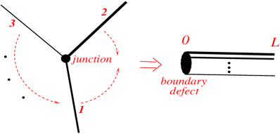
Figure 1: Folding trick

The “boundary defect” representing in the folding trick the junction of wires at $\,x=0\,$ will be described by the boundary condition requiring that the $\,U(1)^{N}$-valued field $\,\bm{g}\,$ belongs to a “brane”:

$$\bm{g}(t,0)\in{\cal B}\equiv\kappa(U(1)^{M})\subset U(1)^{N}\,,$$ (3.3)

where $\,\kappa:U(1)^{M}\rightarrow U(1)^{N}\,$ is a group homomorphism

$$\big{(}e^{{\rm i}\psi_{m}}\big{)}_{{}_{m=1}}^{{}^{M}}\,\mathop{\longmapsto}\limits^{\kappa}\ \big{(}e^{{\rm i}\sum_{m}\kappa_{i}^{m}\psi_{m}}\big{)}_{{}_{i=1}}^{{}^{N}}$$ (3.4)

specified by integers $\kappa^{m}_{i}$. We shall assume that $\kappa$ is injective so that $\kappa(U(1)^{M})\cong U(1)^{M}$.  As may be seen from the Smith normal form of matrix $\,\big{(}\kappa^{m}_{n}\big{)}$, such a property is assured if and only if the $M\times N$ matrix $\big{(}\kappa^{m}_{n}\big{)}$ has rank $M$ and the g.c.d. of its $M\times M$ minors is equal to 1,  see Proposition 4.3 of [44]. In particular, $M\leq N$ necessarily.  Consider matrices $\,T=(T^{mm^{\prime}})\,$ and $\,P=(P_{ii^{\prime}})\,$ defined by the relations

$$T^{mm^{\prime}}=\sum_{i=1}^{N}r_{i}^{2}\kappa^{m}_{i}\kappa^{m^{\prime}}_{i}\,,\qquad P_{ii^{\prime}}=\sum\limits_{m,m^{\prime}=1}^{M}\kappa^{m}_{i}(T^{-1})_{mm^{\prime}}\kappa^{m^{\prime}}_{i^{\prime}}r_{i^{\prime}}^{2}\,.$$ (3.5)

Matrix $\,P\,$ defines the projector on the subspace of $\,\mathbb{R}^{N}$ spanned by the vectors $\,\bm{\kappa}^{m}=(\kappa^{m}_{1},\dots\kappa^{m}_{N})\,$ that is orthogonal with respect to the scalar product

$$\bm{a}\cdot\bm{b}=\sum_{i}r_{i}^{2}a_{i}b_{i}$$ (3.6)

in $\mathbb{R}^{N}$. The boundary condition (3.3) implies that

$$P^{\perp}\partial_{t}\bm{\varphi}(t,0)=0\,,$$ (3.7)

where $\,P^{\perp}\equiv I-P$.  The stationary points of the action functional (3.1) satisfy, besides the imposed boundary conditions, the equations

$$(\partial_{t}^{2}-\partial_{x}^{2})\bm{\varphi}(t,x)=0\,,$$ (3.8)

$$P\,\partial_{x}\bm{\varphi}(t,0)=0\,.$$ (3.9)

Note that relations (3.7) and (3.9) imply mixed Dirichlet-Neumann boundary conditions at $\,x=0\,$ for massless free fields $\,\bm{\varphi}(t,x)$.  The solutions of the classical equations decompose in terms of the left- and right-movers:

$$\bm{\varphi}(t,x)=\bm{\varphi}^{\ell}(t+x)+\bm{\varphi}^{r}(t-x)$$ (3.10)

with

$$\bm{\varphi}^{\ell,r}(t\pm x)\,=\,\bm{\varphi}^{\ell,r}_{0}+\frac{{}_{\pi}}{{}^{2L}}\bm{\alpha}_{0}^{\ell,r}(t\pm x)+{\rm i}\sum\limits_{n\not=0}\frac{{}_{1}}{{}^{n}}\bm{\alpha}^{\ell,r}_{n}{\rm e}^{-\frac{\pi{\rm i}n(t\pm x)}{2L}}\,,$$ (3.11)

where the upper sign relates to the $\bm{\varphi}^{\ell}$ and the lower one to $\bm{\varphi}^{r}$,  and

$$\overline{\bm{\alpha}_{-n}^{\ell,r}}=\bm{\alpha}_{n}^{\ell,r}=(P-P^{\perp})\bm{\alpha}_{n}^{r,\ell}\,,\qquad P\bm{\alpha}_{2n+1}^{\ell,r}=0\,,\qquad P^{\perp}\bm{\alpha}_{2n}^{\ell,r}=0$$ (3.12)

with real $\,\bm{\varphi}_{0}=\bm{\varphi}_{0}^{\ell}+\bm{\varphi}_{0}^{r}\,$ such that $\,{\rm e}^{{\rm i}\bm{\varphi}_{0}}\in{\cal B}$.  In particular, $\,\bm{\alpha}_{2n+1}^{r}=-\bm{\alpha}_{2n+1}^{\ell}\,$ and $\,\bm{\alpha}_{2n}^{r}=\bm{\alpha}_{2n}^{\ell}$.  The space of classical solutions comes equipped with the symplectic form

$$\Omega=\frac{{}_{1}}{{}^{2}}\delta\bm{\alpha}^{\ell}_{0}\cdot\wedge\delta\bm{\varphi}_{0}-\frac{{}_{{\rm i}}}{{}^{2}}\sum_{n\neq 0}\frac{{}_{1}}{{}^{n}}\delta\bm{\alpha}_{n}^{\ell}\cdot\wedge\delta\bm{\alpha}_{-n}^{\ell}$$ (3.13)

which determines the Poisson brackets of functionals on that space that may be directly quantized.

The particular case when $\,\kappa\,$ in (3.4) is the identity mapping of $U(1)^{N}$,  corresponding to the “space-filling” brane ${\cal B}_{0}=U(1)^{M}$,  describes the disconnected wires. In this case, $\,P=I\,$ (i.e. $P$ is the identity matrix) and field $\,\bm{\varphi}\,$ satisfies the Neumann boundary conditions both at $\,x=0\,$ and $\,x=L\,$ and only the even modes $\,\bm{\alpha}_{2n}^{\ell}=\bm{\alpha}_{2n}^{r}\,$ appear. One obtains in this case the product of $N$ theories considered in Sec. 2.3.

4 Quantization

4.1 Space of states

The quantization of the bosonic theory of Sec. 3 is again straightforward but a little more involved than for the disconnected wires. Let us first quantize the zero modes. According to the boundary conditions,

$$\bm{\alpha}^{\ell}_{0}=\bm{\alpha}^{r}_{0}=\sum_{m}\beta_{m}\bm{\kappa}^{m},\qquad\bm{\varphi}_{0}=\sum_{m}\psi_{m}\bm{\kappa}^{m}\,,$$ (4.1)

where $\,(\psi_{m}),\ m=1,\dots,M$,  are angles parameterizing $\,U(1)^{M}$,  so that

$$\frac{{}_{1}}{{}^{2}}\delta\bm{\alpha}^{\ell}_{0}\cdot\wedge\delta\bm{\varphi}_{0}=\frac{{}_{1}}{{}^{2}}\sum_{m,m^{\prime}}T^{mm^{\prime}}\delta\beta_{m}\wedge\delta\psi_{m^{\prime}}\,.$$ (4.2)

The corresponding Poisson brackets are

$$\big{\{}\beta_{m},\,\psi_{m^{\prime}}\big{\}}\,=\,-2(T^{-1})_{mm^{\prime}}$$ (4.3)

leading to the commutators

$$\big{[}\beta_{m},\,\psi_{m^{\prime}}\big{]}\,=\,-2{\rm i}(T^{-1})_{mm^{\prime}}\,.$$ (4.4)

Keeping in mind that the angular variables $\,\psi_{m}\,$ are multivalued, the above commutators will be represented in the Hilbert space $\,{\cal H}_{0}=L^{2}((U(1)^{M})\,$ of functions of $\,M\,$ angles $\,\psi_{m}$,  square integrable in the Haar measure, by setting

$$\beta_{m}=-2{\rm i}\sum_{m^{\prime}}(T^{-1})_{mm^{\prime}}\dfrac{{}_{\partial}}{{}^{\partial\psi_{m^{\prime}}}}\,.$$ (4.5)

An orthonormal basis of $\,{\cal H}_{0}\,$ is given by the states

$$\left|k^{1}\ldots k^{M}\right\rangle\,=\,\exp\Big{(}{\rm i}\sum_{m=1}^{M}k^{m}\psi_{m}\Big{)}\qquad\text{for }\quad k^{m}\in\mathbb{Z}$$ (4.6)

such that

$$\beta_{m}\left|k^{1}\ldots k^{M}\right\rangle=2\sum_{m^{\prime}}(T^{-1})_{mm^{\prime}}k^{m^{\prime}}\left|k^{1}\ldots k^{M}\right\rangle$$ (4.7)

and

$$\bm{\alpha}^{\ell}_{0}\left|k^{1}\ldots k^{M}\right\rangle=2\sum_{m,m^{\prime}}\bm{\kappa}^{m}(T^{-1})_{mm^{\prime}}k^{m^{\prime}}\left|k^{1}\ldots k^{M}\right\rangle.$$ (4.8)

For the excited modes, it is convenient to introduce a basis $\,(\bm{\Lambda}_{j})_{j=1}^{N}$ of vectors $\,\bm{\Lambda}_{j}=(\Lambda_{j1},\dots,\Lambda_{jN})$ in $\,\mathbb{R}^{N}$ such that

$$\bm{\Lambda}_{j}\cdot\bm{\Lambda}_{j^{\prime}}=\delta_{jj^{\prime}},\qquad P\bm{\Lambda}_{j}=\bm{\Lambda}_{j}\quad\text{for}\quad j\leq M\,,\qquad P^{\perp}\bm{\Lambda}_{j}=\bm{\Lambda}_{j}\quad\text{for}\quad j>M$$ (4.9)

and the projected modes

$$\tilde{\alpha}^{\ell,r}_{nj}=\bm{\Lambda}_{j}\cdot\alpha_{n}^{\ell,r}\,.$$ (4.10)

with the inverse formulae

$$\alpha^{\ell,r}_{ni}=\sum\limits_{j=1}^{N}\Lambda_{ji}\,\tilde{\alpha}^{\ell,r}_{nj}\,.$$ (4.11)

Note that relations (3.12) imply that $\,\tilde{\alpha}^{\ell}_{(2n+1)\,j}=0\,$ for $\,j\leq M\,$ and $\,\tilde{\alpha}^{\ell}_{(2n)\,j}=0\,$ for $\,j>M$.  The Poisson brackets of the non-zero operators $\,\tilde{\alpha}_{nj}\,$ take the form

$$\{\tilde{\alpha}^{\ell}_{nj},\tilde{\alpha}^{\ell}_{n^{\prime}j^{\prime}}\}=-{\rm i}n\,\delta_{jj^{\prime}}\delta_{n+n^{\prime},0}$$ (4.12)

leading to the commutators

$$[\tilde{\alpha}^{\ell}_{nj},\tilde{\alpha}^{\ell}_{n^{\prime}j^{\prime}}]=n\,\delta_{jj^{\prime}}\delta_{n+n^{\prime},0}\,.$$ (4.13)

In the standard Fock space quantization, we take

$$\mathcal{F}_{e}=\mathop{\otimes}_{j=1}^{M}\mathcal{F}_{ej},\qquad\qquad\mathcal{F}_{o}=\mathop{\otimes}_{j=M+1}^{N}\mathcal{F}_{oj}$$ (4.14)

where $\mathcal{F}_{ej}$ and $\mathcal{F}_{oj}$ are generated by vectors

$$\tilde{\alpha}_{-(2n_{1})j}^{\ell}\ldots\tilde{\alpha}_{-(2n_{l})j}^{\ell}\left|0\right\rangle_{e}\qquad\qquad l\geq 0,\qquad n_{1}\geq\ldots\geq n_{l}\geq 1,\qquad j\in\{1,\ldots,M\}\,,$$ (4.15)

$$\tilde{\alpha}_{-(2n_{1}+1)j}^{\ell}\ldots\tilde{\alpha}_{-(2n_{l}+1)j}^{\ell}\left|0\right\rangle_{o}\qquad l\geq 0,\qquad n_{1}\geq\ldots\geq n_{l}\geq 0,\qquad j\in\{M+1,\ldots,N\}\$$ (4.16)

with the scalar product determined by the relations

$$\tilde{\alpha}_{(2n)\,j}^{\ell}\left|0\right\rangle_{e}=0\ \quad\text{for }\quad n>0\,,\qquad\tilde{\alpha}_{(2n+1)\,j}^{\ell}\left|0\right\rangle_{o}=0\ \quad\text{for }\quad n\geq 0\,,$$ (4.17)

$${}_{e}\langle 0|0\rangle_{e}={{}_{o}}{\langle}0|0\rangle_{o}=1\,,\qquad{(\tilde{\alpha}_{nj}^{\ell})}^{\dagger}=\tilde{\alpha}_{(-n)j}^{\ell}\,.$$ (4.18)

The total Hilbert space of states of the theory is

$$\mathcal{H}=\mathcal{H}_{0}\otimes\mathcal{F}_{e}\otimes\mathcal{F}_{o}$$ (4.19)

and in the following we identify

$$\left|k^{1}\ldots k^{M}\right\rangle\equiv\left|k^{1}\ldots k^{M}\right\rangle\otimes\left|0\right\rangle_{e}\otimes\left|0\right\rangle_{o}$$ (4.20)

4.2 Currents, charge and energy

We shall be interested in the system that possesses global $U(1)$ symmetry acting on fields by $\,(g_{i}(t,x))\mapsto(ug_{i}(t,x))\,$ for $\,u\in U(1)$.  Invariance of the theory requires that this action preserves the brane $\,{\cal B}=\kappa(U(M))\subset U(N)$.  This holds if and only if the vector $\,\bm{1}=(1,\dots,1)\,$ is in the image of projector $\,P$,  i.e. if $\,P\bm{1}=\bm{1}\,$ or

$$\sum\limits_{i^{\prime}}P_{ii^{\prime}}=1\quad\ \text{for all}\quad i\,.$$ (4.21)

The Noether (electric) current corresponding to the $U(1)$ symmetry has then the form

$$J^{0}(t,x)=\sum\limits_{i=1}^{N}J^{0}_{i}(t,x)\,,\qquad J^{1}(t,x)=\sum\limits_{i=1}^{N}J^{1}_{i}(t,x)$$ (4.22)

in terms of the currents in individual wires with the left-right moving components

$$J_{i}^{\ell,r}(t,x)=\frac{{}_{1}}{{}^{2}}(J^{0}\mp J^{1})(t,x)=\frac{{}_{r_{i}^{2}}}{{}^{2\pi}}\frac{{}_{1}}{{}^{2}}(\partial_{t}\pm\partial_{x})\varphi_{i}(t,x)=\frac{{}_{r_{i}^{2}}}{{}^{4L}}\sum\limits_{n\in{\mathbb{Z}}}\alpha^{\ell,r}_{ni}{\rm e}^{-\frac{\pi{\rm i}n(t\pm x)}{2L}}$$ (4.23)

defining $J_{i}^{\ell}(t,x)$ and $J^{r}(t,x)$ as functions, respectively, of $t+x$ and $t-x$ for any real $t$ and $x$.  We shall use formulae (4.23) also for quantum currents. At $\,x=0$,  the left and right currents are linearly related:

$$J_{i}^{r}(t,0)\,=\,\sum_{i^{\prime}}S_{ii^{\prime}}J_{i^{\prime}}^{\ell}(t,0)\,,$$ (4.24)

where

$$S_{ii^{\prime}}\,=\,P_{i^{\prime}i}-P^{\perp}_{i^{\prime}i}$$ (4.25)

according to (3.12) and the explicit expression (3.5) for the matrix $P$. The $N\times N$  ”$S$-matrix” $S=(S_{ii^{\prime}})$ describes the flow of the currents through the junction of wires. It satisfies the relations

$$S_{i^{\prime}i}=r_{i}^{-2}S_{ii^{\prime}}r_{i^{\prime}}^{2}\,,\qquad\sum_{i^{\prime}}S_{ii^{\prime}}S_{i^{\prime}i"}=\delta_{ii"}\,,\qquad\sum\limits_{i}S_{ii^{\prime}}=1\,,$$ (4.26)

In other words,

$$S_{ii^{\prime}}=r_{i}O_{ii^{\prime}}r_{i^{\prime}}^{-1}$$ (4.27)

where $O=(O_{ii^{\prime}})$ is a symmetric orthogonal matrix such that

$$\sum\limits_{i}r_{i}O_{ii^{\prime}}=r_{i^{\prime}}\,.$$ (4.28)

We shall use matrices $\,S\,$ and $\,O\,$ interchangeably. For $\,N=2$,  there are two possibilities:

$$O\,=\,\Big{(}\begin{matrix}1&0\cr 0&1\end{matrix}\Big{)}\qquad{\rm or}\qquad O\,=\,\frac{1}{r_{1}^{2}+r_{2}^{2}}\Big{(}\begin{matrix}{r_{1}^{2}-r_{2}^{2}}&{2r_{1}r_{2}}\cr{2r_{1}r_{2}}&{r_{2}^{2}-r_{1}^{2}}\end{matrix}\Big{)}.$$ (4.29)

The first case corresponds to the identity embedding $\,\kappa\,$ describing the disconnected wires whereas the second one corresponds to the diagonal embedding of $\,U(1)\,$ into $\,U(1)^{2}\,$ that leads to a nontrivial junction. In the last case, the $r_{1}=r_{2}$ case corresponds to off-diagonal matrix $O=S$ with unit non-zero entries, i.e. to the pure transmission of currents through the junction, but for $\,r_{1}\not=r_{2}\,$ the currents are partly transmitted and partly reflected at the junction.

Eq. (4.24) implies that the right currents are linear combinations of left currents if considered as functions of real $t$ and $x$:

$$J_{i}^{r}(t,x)=\sum_{i^{\prime}}S_{ii^{\prime}}J_{i^{\prime}}^{\ell}(t,-x)\,.$$ (4.30)

At $\,x=L$,  i.e. at the ends of the wires, the left and right currents are equal:

$$J_{i}^{r}(t,L)=J_{i}^{\ell}(t,L)$$ (4.31)

which implies that

$$J_{i}^{r}(t,x)=J_{i}^{\ell}(t,-x+2L)$$ (4.32)

if we treat the currents as functions of real $t$ and $x$.  The quantum currents satisfy the equal-time commutation relations

$$[J^{\ell}_{i}(t,x),J^{\ell}_{i^{\prime}}(t,y)] =\frac{{}_{{\rm i}r_{i}^{2}}}{{}^{4\pi}}\sum_{n\in\mathbb{Z}}\big{(}P_{ii^{\prime}}+(-1)^{n}(\delta_{ii^{\prime}}-P_{ii^{\prime}})\big{)}\,\delta^{\prime}(x-y+2nL)$$ (4.33)

$$=-[J^{r}_{i}(t,x),J^{r}_{i^{\prime}}(t,y)]\,,$$ (4.34)

$$[J^{\ell}_{i}(t,x),J^{r}_{i^{\prime}}(t,y)] =\frac{{}_{{\rm i}r_{i}^{2}}}{{}^{4\pi}}\sum_{n\in\mathbb{Z}}\big{(}P_{ii^{\prime}}-(-1)^{n}(\delta_{ii^{\prime}}-P_{ii^{\prime}})\big{)}\,\delta^{\prime}(x+y+2nL)\,,$$ (4.36)

In particular, the left-moving currents commute among themselves at equal times if their positions do not coincide modulo $2L$. Similarly for the right-moving currents. The left-moving currents commute with the right-moving ones at equal times if their positions are not opposite modulo $2L$. Note that for $\,0<x,y\leq L$ the only terms that contribute to (4.34) and (4.36) have $n=0$ or $n=1$, respectively, so that for such values of $x$ and $y$ the commutation relations of currents do not depend on the choice of brane ${\cal B}$. This permits to identify for different junctions the algebras of observables generated by currents $J^{\ell,r}_{i}(0,x)$ with $0<x\leq L$, i.e. localized away from the contact point. In particular, we may identify such observables for disconnected wires with those for connected wires, with the physical meaning that their measurement just before and just after establishing or breaking the connection between the wires should give the same result.  Whatever the junction, the total charge

$$Q(t)=\sum\limits_{i=1}^{N}Q_{i}(t)\,,$$ (4.37)

where $Q_{i}(t)$ are the charges in the individual wires,

$$Q_{i}(t)=\int\limits_{0}^{L}J^{0}_{i}(t,x)\,{\rm d}x\,,$$ (4.38)

is conserved:

$$\dfrac{{\rm d}Q(t)}{{\rm d}t}=\sum_{i=1}^{N}\int\limits_{0}^{L}(\partial_{t}J_{i}^{\ell}(t,x)+\partial_{t}J_{i}^{r}(t,x)){\rm d}x$$ (4.39)

$$=\sum_{i=1}^{N}\int\limits_{0}^{L}(\partial_{x}J_{i}^{\ell}(t,x)-\partial_{x}J_{i}^{r}(t,x)){\rm d}x=\sum_{i=1}^{N}\left[J_{i}^{\ell}(t,x)-J_{i}^{r}(t,x)\right]_{x=0}^{x=L}$$ (4.40)

$$=2\sum_{i,i^{\prime}=1}^{N}(\delta_{ii^{\prime}}-P_{i^{\prime}i})J^{\ell}_{i^{\prime}}(t,0)=0$$ (4.41)

due to (4.21). In terms of the modes,

$$Q=\sum_{i}\frac{{}_{r_{i}^{2}}}{{}^{2}}\alpha_{0i}^{\ell}\,.$$ (4.42)

Operator $\,Q\,$ acts only on $\,\mathcal{H}_{0}\,$:

$$Q\left|k^{1}\ldots k^{M}\right\rangle=\sum_{i}\sum_{m,m^{\prime}}r_{i}^{2}\kappa_{i}^{m}(T^{-1})_{mm^{\prime}}k^{m^{\prime}}\left|k^{1}\ldots k^{M}\right\rangle=(\bm{p},T^{-1}\bm{k})\left|k^{1}\ldots k^{M}\right\rangle,$$ (4.43)

where $\,\bm{p}=(p^{m})\in\mathbb{R}^{M}\,$ with

$$p^{m}=\sum_{i}r_{i}^{2}\kappa_{i}^{m}=\bm{1}\cdot\bm{\kappa}^{m}\,,$$ (4.44)

and

$$(\bm{a},\bm{b})=\sum_{m}a^{m}b^{m}\,,$$ (4.45)

denotes the standard scalar product on $\mathbb{R}^{M}$, to be distinguished from the one of (3.6) used in $\mathbb{R}^{N}$.  Note that the spectrum of $\,Q\,$ is composed of integers, as must be the case for the generator of a unitary action of $\,U(1)\,$ group.  Indeed, since for each $1\leq i\leq N$,

$$\sum\limits_{m,m^{\prime}=1}^{M}p^{m}(T^{-1})_{mm^{\prime}}\kappa^{m^{\prime}}_{i}=(P\bm{1})_{i}=1$$ (4.46)

by (4.21), the injectivity of the homomorphism (3.4) implies that the sums $\sum\limits_{m}p^{m}(T^{-1})_{mm^{\prime}}$ are integers. This is not the case for (non-conserved) charges in the individual wires

$$Q_{i}(t)=\int\limits_{0}^{L}J^{0}_{i}(t,x)\,{\rm d}x=\frac{{}_{r_{i}^{2}}}{{}^{2}}\,\alpha_{0i}^{\ell}-\frac{{}_{{\rm i}r_{i}^{2}}}{{}^{\pi}}\sum\limits_{n}\frac{{}_{1}}{{}^{2n+1}}\,\alpha^{\ell}_{(2n+1)i}\,{\rm e}^{-\frac{\pi{\rm i}(2n+1)t}{2L}}.$$ (4.47)

The energy of the bosonic system of Sec. 3 is given by its classical Hamiltonian that may be expressed in terms of the left and right moving currents by the formula

$$H(t)=\sum_{i=1}^{N}\frac{{}_{2\pi}}{{}^{r_{i}^{2}}}\int\limits_{0}^{L}\big{(}(J_{i}^{\ell}(t,x))^{2}+(J_{i}^{r}(t,x))^{2}\big{)}\,{\rm d}x\,.$$ (4.48)

Its conservation, that holds independently of the condition (4.21), results from the identity

$$\dfrac{{\rm d}H(t)}{{\rm d}t}=\sum_{i=1}^{N}2\pi r_{i}^{-2}\left[(J_{i}^{\ell})^{2}(t,x)-(J_{i}^{r})^{2}(t,x)\right]_{x=0}^{x=L}$$ (4.49)

whose right hand side vanishes because

$$(J_{i}^{r})^{2}(t,L)=(J_{i}^{\ell})^{2}(t,L)$$ (4.50)

for all $1\leq i\leq N$,  and because

$$\sum_{i=1}^{N}r_{i}^{-2}(J_{i}^{r})^{2}(t,0)=\sum_{i,i^{\prime},i"=1}^{N}r_{i}^{-2}S_{ii^{\prime}}S_{ii"}J_{i^{\prime}}^{\ell}(t,0)J_{i"}^{\ell}(t,0)=\sum_{i=1}^{N}r_{i}^{-2}(J_{i}^{\ell})^{2}(t,0)$$ (4.51)

in virtue of (4.26).  The quantum Hamiltonian $\,H\,$ is given by the Wick reordered version of the classical expression:

$$H=\sum_{i=1}^{N}\frac{{}_{2\pi}}{{}^{r_{i}^{2}}}\int\limits_{0}^{L}(:J_{i}^{\ell}(t,x)^{2}:+:J_{i}^{r}(t,x)^{2}:)\,{\rm d}x\,+\frac{{}_{\pi}}{{}^{L}}\frac{{}_{N-3M}}{{}^{48}}$$ (4.52)

$$=\frac{{}_{\pi}}{{}^{4L}}\,\bm{\alpha}^{\ell}_{0}\cdot\bm{\alpha}^{\ell}_{0}+\frac{{}_{\pi}}{{}^{2L}}\sum_{i=1}^{M}\sum_{n>0}\tilde{\alpha}_{(-2n)i}^{\ell}\tilde{\alpha}_{(2n)i}^{\ell}+\frac{{}_{\pi}}{{}^{2L}}\sum_{i=M+1}^{N}\sum_{n\geq 0}\tilde{\alpha}_{(-(2n+1))i}^{\ell}\tilde{\alpha}_{(2n+1)i}^{\ell}\,\,+\frac{{}_{\pi}}{{}^{L}}\frac{{}_{N-3M}}{{}^{48}}\,,\qquad\,,$$ (4.53)

where the last c-number term accounts for the $\zeta$-function regularized zero-point energy of the excited modes:

$$\frac{{}_{\pi}}{{}^{2L}}\frac{{}_{M}}{{}^{2}}\sum_{n=1}^{\infty}2n+\frac{{}_{\pi}}{{}^{2L}}\frac{{}_{N-M}}{{}^{2}}\sum\limits_{n=0}^{\infty}(2n+1)=\frac{{}_{\pi}}{{}^{2L}}\frac{{}_{3M-N}}{{}^{2}}\,\zeta(-1)=\frac{{}_{\pi}}{{}^{L}}\frac{{}_{N-3M}}{{}^{48}}.$$ (4.54)

The Hilbert space vectors

$$\left|u\right\rangle=\tilde{\alpha}_{-(2n^{j_{1}}_{1})j_{1}}^{\ell}\ldots\tilde{\alpha}_{-(2n^{j_{l}}_{l})j_{l}}^{\ell}\tilde{\alpha}_{-(2n^{j^{\prime}_{1}}_{1}+1)j^{\prime}_{1}}^{\ell}\ldots\tilde{\alpha}_{-(2n^{j^{\prime}_{l^{\prime}}}_{l^{\prime}}+1)j^{\prime}_{l^{\prime}}}^{\ell}\left|k_{1}\ldots k_{M}\right\rangle$$ (4.55)

with $j_{1},\dots,j_{l}\leq M$ and $j^{\prime}_{1},\dots,j^{\prime}_{l^{\prime}}>M\,$ form a basis of eigen-states of $H$ with

$$H\left|u\right\rangle=\frac{{}_{\pi}}{{}^{2L}}\left(2\,(\bm{k},T^{-1}\bm{k})+n+\frac{{}_{N-3M}}{{}^{24}}\right)\left|u\right\rangle\,,$$ (4.56)

where

$$n=\sum_{k=1}^{l}2n^{j_{k}}_{k}+\sum_{k^{\prime}=1}^{l^{\prime}}(2n^{j^{\prime}_{k^{\prime}}}_{k^{\prime}}+1)\,.$$ (4.57)

The energy density and the energy current in the wires correspond, respectively, to operators $\,K^{0}_{i}(t,x)=T^{r}_{i}(t,x)+T^{\ell}_{i}(t,x)\,$ and $\,K^{1}_{i}(t,x)=T^{r}_{i}(t,x)-T^{\ell}_{i}(t,x)$,  where

$$T^{\ell}_{i}(t,x)=\frac{{}_{2\pi}}{{}^{r_{i}^{2}}}:J_{i}^{\ell}(t,x)^{2}:-\,\frac{{}_{\pi}}{{}^{48L^{2}}}P_{ii}\,+\,\frac{{}_{\pi}}{{}^{96L^{2}}}P^{\perp}_{ii}\,,$$ (4.58)

$$T^{r}_{i}(t,x)=\frac{{}_{2\pi}}{{}^{r_{i}^{2}}}:J_{i}^{r}(t,x)^{2}:-\,\frac{{}_{\pi}}{{}^{48L^{2}}}P_{ii}\,+\,\frac{{}_{\pi}}{{}^{96L^{2}}}P^{\perp}_{ii}\,,$$ (4.59)

are the left-moving and right-moving energy-momentum-tensor components. The constant terms are the zero-point energy contributions. Note that the above choice assures by virtue of relation $\,\sum\limits_{i=1}^{N}P_{ii}=M\,$ that

$$H=\sum\limits_{i=1}^{N}H_{i}(t)\,,$$ (4.60)

where

$$H_{i}(t)=\int\limits_{0}^{L}K_{i}^{0}(t,x)\,{\rm d}x$$ (4.61)

are the observables representing energy in individual wires.

5 Equilibrium state.

The equilibrium state at inverse temperature $\beta$ and (electric) potential $\,V\,$ is described by the density matrix

$$\rho_{\beta,V}=\frac{1}{Z_{\beta,V}}\,{\rm e}^{-\beta(H-VQ)}\,,$$ (5.1)

where $\,Z_{\beta,V}\,$ is the the partition function. Note that with our conventions, positive $\,V\,$ plays the role of a positive chemical potential for electrons and of a negative one for holes. $\,Z_{\beta,V}\,$ is easily calculable with the use of relations (4.56) and (4.43):

$$Z_{\beta,V}={\rm Tr}_{\mathcal{H}}\Big{(}{\rm e}^{-\beta(H-VQ)}\Big{)}$$ (5.2)

$$={\rm e}^{-\frac{(N-3M)\pi\beta}{48L}}\bigg{(}\sum_{\bm{k}\in\mathbb{Z}^{M}}{\rm e}^{-\frac{\pi\beta}{L}(\bm{k},T^{-1}\bm{k})+\beta V(\bm{p},T^{-1}\bm{k})}\bigg{)}\bigg{(}\sum_{n\geq 0}p_{e}(n)\,{\rm e}^{-\frac{\pi\beta}{2L}n}\bigg{)}^{M}\bigg{(}\sum_{n\geq 0}p_{o}(n)\,{\rm e}^{-\frac{\pi\beta}{2L}n}\bigg{)}^{N-M}\ \quad$$ (5.3)

with $p_{e}(n)$ ($p_{o}(n)$) standing for the number of partitions of $n$ into a sum of even (odd) numbers. The Poisson resummation formula applied to the $\bm{k}$-sum and the standard relation of the generating function for partitions to the Dedekind function $\,\eta(\tau)={\rm e}^{\frac{\pi i\tau}{12}}\prod\limits_{n=1}^{\infty}\big{(}1-{\rm e}^{2\pi{\rm i}\tau n}\big{)}\,$ allow to rewrite (5.3) as

$$Z_{\beta,V}=\Big{(}\frac{{}_{L}}{{}^{\beta}}\Big{)}^{\frac{M}{2}}\sqrt{\det(T)}\ {\rm e}^{\frac{L\beta V^{2}}{4\pi}\sum_{i}r_{i}^{2}}\bigg{(}\sum_{\bm{k}\in\mathbb{Z}^{M}}{\rm e}^{-{\rm i}LV(\bm{p},\bm{k})-\frac{\pi L}{\beta}(\bm{k},T\bm{k})}\bigg{)}\big{[}\eta(\frac{{}_{{\rm i}\beta}}{{}^{2L}})\big{]}^{N-2M}\big{[}\eta(\frac{{}_{{\rm i}\beta}}{{}^{4L}})\big{]}^{M-N},$$ (5.4)

or, with the use of the modular property of $\,\eta(\tau)=\frac{1}{\sqrt{-i\tau}}\eta(-\frac{1}{\tau})$,  as

$$Z_{\beta,V}=2^{-N}\sqrt{\det(T)}\ {\rm e}^{\frac{L\beta V^{2}}{4\pi}\sum_{i}r_{i}^{2}}\bigg{(}\sum_{\bm{k}\in\mathbb{Z}^{M}}{\rm e}^{-{\rm i}LV(\bm{p},\bm{k})-\frac{\pi L}{\beta}(\bm{k},T\bm{k})}\bigg{)}\big{[}\eta(\frac{{}_{2{\rm i}L}}{{}^{\beta}})\big{]}^{N-2M}\big{[}\eta(\frac{{}_{4{\rm i}L}}{{}^{\beta}})\big{]}^{M-N}.$$ (5.5)

The equilibrium state $\,\omega^{L}_{\beta,V}$ expectations of the observable algebra generated by currents $J^{\ell,r}_{i}$ are defined by the formula

$$\omega^{L}_{\beta,V}(A)={\rm Tr}\big{(}\rho_{\beta,V}A\big{)}\,.$$ (5.6)

The superscript $L$ in $\,\omega^{L}_{\beta,V}$ stresses that the state pertains to the junction of wires of length $L$. In forming observables, it is enough to consider only the currents $J^{\ell}(t,x)$ at fixed $t$ and real $x$. We shall decompose such currents into the contributions from the zero modes and the excited modes:

$$J^{\ell}_{i}(t,x)=\frac{{}_{r_{i}^{2}}}{{}^{4L}}\alpha^{\ell}_{0i}+\hat{J}^{\ell}_{i}(t,x)\,,$$ (5.7)

see (4.23). In the equilibrium state expectation of products of currents, the contributions from the zero modes and from the excited modes factorize. In particular,

$$\omega^{L}_{\beta,V}\Big{(}\prod\limits_{k=1}^{K}\frac{{}_{r_{i_{k}}^{2}}}{{}^{2L}}\,\alpha_{0i_{k}}^{\ell}\Big{)} =\frac{1}{(2\beta VL)^{K}}\,\dfrac{\prod\limits_{k=1}^{K}\big{(}r_{i_{k}}^{2}\sum\limits_{m}\kappa^{m}_{i_{k}}\frac{\partial}{\partial p^{m}}\big{)}\sum\limits_{\bm{k}\in\mathbb{Z}^{M}}\,{\rm e}^{-\frac{\pi\beta}{L}(\bm{k},T^{-1}\bm{k})+\beta V(\bm{p},T^{-1}\bm{k})}}{\sum\limits_{\bm{k}\in\mathbb{Z}^{M}}{\rm e}^{-\frac{\pi\beta}{L}(\bm{k},T^{-1}\bm{k})+\beta V(\bm{p},T^{-1}\bm{k})}}$$ (5.8)

$$=\frac{1}{(2\beta VL)^{K}}\,\dfrac{\prod\limits_{k=1}^{K}\big{(}r_{i_{k}}^{2}\sum\limits_{m}\kappa^{m}_{i_{k}}\frac{\partial}{\partial p^{m}}\big{)}\,\,\big{(}{\rm e}^{\frac{L\beta V^{2}}{4\pi}(\bm{p},T^{-1}\bm{p})}\sum\limits_{\bm{k}\in\mathbb{Z}^{M}}{\rm e}^{-{\rm i}LV(\bm{p},\bm{k})-\frac{\pi L}{\beta}(\bm{k},T\bm{k})}\big{)}}{{\rm e}^{\frac{L\beta V^{2}}{4\pi}(\bm{p},T^{-1}\bm{p})}\sum\limits_{\bm{k}\in\mathbb{Z}^{M}}{\rm e}^{-\frac{{\rm i}LV}{2}(\bm{p},\bm{k})-\frac{\pi L}{\beta}(\bm{k},T\bm{k})}}\,,\quad$$ (5.9)

where the second equality results from the Poisson resummation. On the other hand, the expectations of products of $\hat{J}^{+}_{i}$ are calculated by the Wick rule with

$$\omega^{L}_{\beta,V}\big{(}\hat{J}^{\ell}_{i}(t,x)\big{)}=0\,,$$ (5.10)

$$\omega^{L}_{\beta,V}\big{(}\hat{J}^{\ell}_{i_{1}}(t,x_{1})\,\hat{J}^{\ell}_{i_{2}}(t,x_{2})\big{)}=-\frac{{}_{1}}{{}^{2}}\left(\frac{{}_{r_{i_{1}}}}{{}^{2\pi}}\right)^{2}\Big{(}P_{i_{1}i_{2}}\,f_{e}(x_{1}-x_{2})+(\delta_{i_{1}i_{2}}-P_{i_{1}i_{2}})f_{o}(x_{1}-x_{2})\Big{)},\quad$$ (5.11)

where

$$f_{e}(x_{1}-x_{2}) =\wp(x_{1}-x_{2};2L,-{\rm i}\beta)+C_{e}$$ (5.12)

$$f_{o}(x_{1}-x_{2}) =2{\wp}(x_{1}-x_{2};4L,-{\rm i}\beta)-{\wp}(x_{1}-x_{2};2L,-{\rm i}\beta)+C_{o}$$ (5.13)

with the constants

$$C_{e}= \big{(}\frac{{}_{\pi}}{{}^{2L}}\big{)}^{2}\Big{(}\frac{{}_{1}}{{}^{3}}-\sum\limits_{n\neq 0}\sinh^{-2}(\frac{{}_{\pi n\beta}}{{}^{2L}})\Big{)},$$ (5.14)

$$C_{o}= \big{(}\frac{{}_{\pi}}{{}^{2L}}\big{)}^{2}\Big{(}-\frac{{}_{1}}{{}^{6}}-\frac{{}_{1}}{{}^{2}}\sum\limits_{n\neq 0}\sinh^{-2}(\frac{{}_{\pi n\beta}}{{}^{4L}})+\sum\limits_{n\neq 0}\sinh^{-2}(\frac{{}_{\pi n\beta}}{{}^{2L}})\Big{)}.$$ (5.15)

Above, $\wp(z;\omega_{1},\omega_{2})=\wp(z;\omega_{2},\omega_{1})$ is the Weierstrass function of period $\omega_{1}$ and $\omega_{2}$ [47]:

$$\wp(z;\omega_{1},\omega_{2}) =\frac{{}_{1}}{{}^{z^{2}}}\,+\sum_{n^{2}+m^{2}\neq 0}\Big{(}\frac{{}_{1}}{{}^{(z+m\omega_{1}+n\omega_{2})^{2}}}-\frac{{}_{1}}{{}^{\left(m\omega_{1}+n\omega_{2}\right)^{2}}}\Big{)}$$ (5.16)

$$=(\frac{{}_{\pi}}{{}^{\omega_{2}}})^{2}\Big{[}-\frac{{}_{1}}{{}^{3}}+\sum\limits_{n}\sin^{-2}\big{(}\frac{{}_{\pi(z-n\omega_{1})}}{{}^{\omega_{2}}}\big{)}-\sum\limits_{n\not=0}\sin^{-2}\big{(}\frac{{}_{\pi n\omega_{1}}}{{}^{\omega_{2}}}\big{)}\Big{]}.$$ (5.17)

Note the singularity of the 2-point functions (5.11) at the insertion points coinciding modulo $2L$. For such points, the equal-time commutators of currents have contact terms, see (4.34).  For the 1-point function of the left current, one obtains

$$\omega^{L}_{\beta,V}\left(J_{i}^{\ell}(t,x)\right)=\frac{{}_{r_{i}^{2}V}}{{}^{4\pi}}-\frac{{}_{{\rm i}r_{i}^{2}}}{{}^{2\beta}}\sum_{m}\kappa_{i}^{m}\,\dfrac{\displaystyle\sum_{\bm{k}\in\mathbb{Z}^{M}}k^{m}{\rm e}^{-{\rm i}LV(\bm{p},\bm{k})-\frac{\pi L}{\beta}(\bm{k},T\bm{k})}}{\displaystyle\sum_{\bm{k}\in\mathbb{Z}^{M}}{\rm e}^{-{\rm i}LV(\bm{p},\bm{k})-\frac{\pi L}{\beta}(\bm{k},T\bm{k})}}\,,$$ (5.18)

where we have used the relation

$$\frac{{}_{r_{i}^{2}}}{{}^{2L\beta V}}\sum_{m}\kappa_{i}^{m}\frac{{}_{\partial\,}}{{}^{\partial p^{m}}}\big{(}\frac{{}_{L\beta V^{2}}}{{}^{4\pi}}(\bm{p},T^{-1}\bm{p})\big{)}=\frac{{}_{r_{i}^{2}V}}{{}^{4\pi}}\sum_{m,m^{\prime}}\kappa_{i}^{m}(T^{-1})_{mm^{\prime}}p^{m^{\prime}}=\frac{{}_{r_{i}^{2}V}}{{}^{4\pi}}\sum_{j}P_{ij}=\frac{{}_{r_{i}^{2}V}}{{}^{4\pi}}\,.$$ (5.19)

From (4.32) or (4.30), it follows that $\,\omega^{L}_{\beta,V}\left(J_{i}^{r}(t,x)\right)=\omega^{L}_{\beta,V}\left(J_{i}^{\ell}(t,x)\right)\,$ so that

$$\omega^{L}_{\beta,V}\left(J_{i}^{0}(t,x)\right)=2\,\omega^{L}_{\beta,V}\left(J_{i}^{\ell}(t,x)\right)\,,\qquad\omega^{L}_{\beta,V}\left(J_{i}^{1}(t,x)\right)=0\,.$$ (5.20)

Hence, in the equilibrium state, the mean charge density is constant in each wire, whereas the mean current vanishes.

The equilibrium state $\,\omega^{L}_{\beta,V}$ is invariant under the replacement $J^{\ell}\leftrightarrow J^{r}$,  the property expressing its time-reversal invariance. For the energy-momentum tensor components $T_{i}^{\ell,r}(t,x)$ defined by (4.58) and (4.59),  we obtain:

$$\omega^{L}_{\beta,V}\big{(}T_{i}^{\ell}(t,x)\big{)} =\frac{{}_{\pi}}{{}^{8L^{2}}}r_{i}^{2}\,\omega^{L}_{\beta,V}\big{(}(\alpha_{0i}^{+})^{2}\big{)}\,-\,\frac{{}_{1}}{{}^{4\pi}}\big{(}P_{ii}C_{e}+(1-P_{ii})C_{o}\big{)}$$ (5.21)

$$=\lim\limits_{\epsilon\to 0}\,\omega^{L}_{\beta,V}\Big{(}\frac{{}_{2\pi}}{{}^{r_{i}^{2}}}\,J^{\ell}_{i}(t,x+\epsilon)\,J^{\ell}_{i}(t,x)\,+\,\frac{{}_{1}}{{}^{4\pi\epsilon^{2}}}\Big{)}$$ (5.22)

$$=\lim\limits_{\epsilon\to 0}\,\omega^{L}_{\beta,V}\Big{(}\frac{{}_{2\pi}}{{}^{r_{i}^{2}}}\,J^{r}_{i}(t,x+\epsilon)\,J^{r}_{i}(t,x)\,+\,\frac{{}_{1}}{{}^{4\pi\epsilon^{2}}}\Big{)}\,=\,\omega^{L}_{\beta,V}\big{(}T_{i}^{r}(t,x)\big{)},$$ (5.23)

which is a consequence of the operator product expansion

$$\frac{{}_{2\pi}}{{}^{r_{i}^{2}}}\,J^{\ell}_{i}(t,x+\epsilon)\,J^{\ell}_{i}(t,x)=-\frac{{}_{1}}{{}^{4\pi\epsilon^{2}}}+T_{i}^{\ell}(t,x)\,+\,\dots$$ (5.24)

$$\frac{{}_{2\pi}}{{}^{r_{i}^{2}}}\,J^{r}_{i}(t,x+\epsilon)\,J^{r}_{i}(t,x)=-\frac{{}_{1}}{{}^{4\pi\epsilon^{2}}}+T_{i}^{r}(t,x)\,+\,\dots$$ (5.25)

holding under the equilibrium expectations away from other insertions points.

6 Functional integral representation

6.1 Case with $\,V=0$

For $\,V=0$,  the partition function $\,Z_{\beta,0}\equiv Z_{\beta}\,$ and the expectations in the thermal equilibrium states $\,\omega^{L}_{\beta,0}\equiv\omega^{L}_{\beta}\,$ may be represented by Euclidean functional integrals over a cylindrical open-string worldsheet,  see Fig. 2.

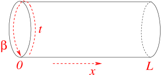
Figure 2: Open string worldsheet

For the partition function,

$$Z_{\beta}=\int{\rm e}^{-S_{E}[g]}\,{\cal D}g$$ (6.1)

where the functional integral is over the maps $\,\bm{g}(t,x)=({\rm e}^{i\varphi_{i}(t,x)})\,$ from $\mathbb{R}\times[0,L]$ to $U(1)^{N}$ periodic in $t$

$$\bm{g}(t+\beta,x)=\bm{g}(t,x)$$ (6.2)

with the boundary conditions

$$\bm{g}(t,0)\in{\cal B}\,,\qquad P(\bm{g}^{-1}\partial_{x}\bm{g})(t,0)=0\,,\qquad(\bm{g}^{-1}\partial_{x}\bm{g})(t,L)=0$$ (6.3)

and the Euclidean action functional

$$S_{E}[\bm{g}]\,=\,\frac{{}_{1}}{{}^{4\pi}}\sum\limits_{i=1}^{N}\int\limits_{0}^{\beta}{\rm d}t\int\limits_{0}^{L}r_{i}^{2}\big{(}(\partial_{t}\varphi_{i})^{2}+(\partial_{x}\varphi_{i})^{2}\big{)}(t,x)\,{\rm d}x\,\equiv\,S_{E}[\bm{\varphi}]\,.$$ (6.4)

To give sense to the functional integrals,  one decomposes the multivalued fields $\,\varphi_{i}(t,x)\,$ into the linear part which winds in the time direction and the periodic part:

$$\varphi_{i}(t,x)=\frac{{}_{2\pi}}{{}^{\beta}}n_{i}t+\tilde{\varphi}_{i}(t,x)\,,$$ (6.5)

where

$$n_{i}=\sum\limits_{m=1}^{M}\kappa^{m}_{i}q_{m}\,,\qquad\tilde{\varphi}_{i}(t,0)=\sum\limits_{m=1}^{M}\kappa^{m}_{i}\tilde{\psi}_{m}(t)\,,\qquad P\,\partial_{x}\tilde{\bm{\varphi}}(t,0)=0=\partial_{x}\tilde{\bm{\varphi}}(t,L)$$ (6.6)

with $\,q_{m}\in\mathbb{Z}$, $\,\tilde{\psi}_{m}\in\mathbb{R}$,  and with the multivaluedness reduced to that of $\,\tilde{\psi}_{m}$ defined modulo $2\pi$. The Euclidean action functional decomposes accordingly:

$$S_{E}[\bm{\varphi}]=\frac{{}_{\pi L}}{{}^{\beta}}\,(\bm{k},T\bm{k})+S_{E}(P\tilde{\bm{\varphi}})+S_{E}((I-P)\tilde{\bm{\varphi}})$$ (6.7)

leading to the factorization of the functional integral

$$\int{\rm e}^{-S_{E}[\bm{g}]}\,{\cal D}\bm{g}=\sum\limits_{\bm{k}\in\mathbb{Z}^{M}}{\rm e}^{-\frac{\pi L}{\beta}\,(\bm{k},T\bm{k})}\,\int{\rm e}^{-S_{E}[P\tilde{\bm{\varphi}}]}\,{\cal D}(P\tilde{\bm{\varphi}})\,\int{\rm e}^{-S_{E}[(I-P)\tilde{\bm{\varphi}}]}\,{\cal D}((I-P)\tilde{\bm{\varphi}})\,.$$ (6.8)

The last factor is a standard Gaussian functional integral with the quadratic form corresponding to the Laplacian with the periodic boundary conditions in the $t$ direction and the mixed Dirichlet one at $x=0$ and the Neumann one at $x=L$ in the $x$ direction. Such Laplacian is strictly positive. Using the zeta-function regularization of such an infinite-dimensional Gaussian integral, one obtains:

$$\int{\rm e}^{-S_{E}({\rm e}^{{\rm i}(I-P)\tilde{\bm{\varphi}}})}\,{\cal D}((I-P)\tilde{\bm{\varphi}})=\left|\eta\big{(}\frac{{}_{{\rm i}\beta}}{{}^{2L}}\big{)}\right|^{N-M}\left|\eta\big{(}\frac{{}_{{\rm i}\beta}}{{}^{4L}}\big{)}\right|^{-(N-M)}.$$ (6.9)

In the first functional integral on the right hand side of (6.8), we parameterize

$$P\tilde{\bm{\varphi}}=\sum\limits_{m=1}^{M}\tilde{\psi}_{m}\bm{\kappa}^{m}\,.$$ (6.10)

$S_{E}[P\tilde{\bm{\varphi}}]$ becomes then a quadratic form in $(\tilde{\psi}_{m})$ corresponding to the Laplacian with the periodic boundary conditions in the $t$ direction and the Neumann ones in the $x$ direction, with constant zero modes. The zero-mode integration may be turned to a one over $U(1)^{M}$ using collective coordinates and recalling that fields $\tilde{\psi}_{m}$ are determined modulo $2\pi$. Employing the zeta-function regularization for the remaining Gaussian functional integral over the other modes, one obtains

$$\int{\rm e}^{-S_{E}[P\tilde{\bm{\varphi}}]}\,{\cal D}(P\tilde{\bm{\varphi}})=\sqrt{\det T}\,\Big{(}\frac{{}_{L}}{{}^{\beta}}\Big{)}^{\frac{M}{2}}\left|\eta\big{(}\frac{{}_{{\rm i}\beta}}{{}^{2L}}\big{)}\right|^{-M}.$$ (6.11)

Upon the substitution of (6.9) and (6.11) to (6.7),  the functional integral expression (6.1) for $\,Z_{\beta}\,$ reduces to (5.4) with $\,V=0$.

The expectations of products of equal-time currents in the thermal state $\,\omega^{L}_{\beta}\,$ are represented by the normalized functional integrals:

$$\omega^{L}_{\beta}\Big{(}\prod\limits_{k=1}^{K}J_{i_{k}}^{\ell}(t,x_{k})\prod\limits_{k^{\prime}=1}^{K^{\prime}}J_{i_{k^{\prime}}}^{r}(t,y_{k^{\prime}})\Big{)}=\frac{1}{Z_{\beta}}\int\prod\limits_{k}j_{i_{k}}^{\ell}(0,x_{k})\prod\limits_{k^{\prime}}j_{i_{k^{\prime}}}^{r}(0,y_{k^{\prime}})\,\,{\rm e}^{-S_{E}(\bm{g})}\,{\cal D}\bm{g}\,,$$ (6.12)

where on the right hand side

$$j^{\ell}_{i}(t,x)=\frac{{}_{r_{i}^{2}}}{{}^{2\pi}}\frac{{}_{1}}{{}^{2}}(\partial_{x}-i\partial_{t})\varphi_{i}(t,x)\,,\qquad j^{r}_{i}(t,x)=-\frac{{}_{r_{i}^{2}}}{{}^{2\pi}}\frac{{}_{1}}{{}^{2}}(\partial_{x}+i\partial_{t})\varphi_{i}(t,x)\,,$$ (6.13)

are functionals of field $\,\bm{\varphi}(t,x)\,$ that in terms of decomposition (6.5) take the form

$$j^{\ell}_{i}(t,x)=-i\frac{{}_{r_{i}^{2}n_{i}}}{{}^{2\beta}}+\frac{{}_{r_{i}^{2}}}{{}^{2\pi}}\frac{{}_{1}}{{}^{2}}(\partial_{x}-i\partial_{t})\tilde{\varphi}_{i}(t,x)\,,\quad\ j^{r}_{i}(t,x)=-i\frac{{}_{r_{i}^{2}n_{i}}}{{}^{2\beta}}-\frac{{}_{r_{i}^{2}}}{{}^{2\pi}}\frac{{}_{1}}{{}^{2}}(\partial_{x}+i\partial_{t})\tilde{\varphi}_{i}(t,x)\,.\$$ (6.14)

The functional integral (6.12) factorizes similarly as in (6.8), with terms $-i\frac{r_{i}^{2}n_{i}}{2\beta}=-i\frac{r_{i}^{2}}{2\beta}\sum\limits_{m}\kappa^{m}_{i}k_{m}$ contributing to the factor with the sum over $\,\bm{k}\,$ and terms with derivatives of $\,\tilde{\bm{\varphi}}\,$ entering the factors involving the Gaussian integrals calculated by the Wick rule. The latter leads to combinations of products of derivatives of the Green functions of the Laplacians that reduce to expressions involving the Weierstrass functions. At the end, one obtains the same formulae as the $\,V\to 0\,$ limit of the ones worked out before for the expectations of products of the left-moving currents resulting from applying the rule (4.30) to the right-moving currents.

6.2 General case

An imaginary potential $\,V\,$ may be included in the functional integral approach by imposing the twisted-periodic boundary conditions in the time direction on the $U(1)^{N}$-valued fields $\,\bm{g}=(g_{i})=({\rm e}^{i\varphi_{i}})$:

$$g_{i}(t+\beta,x)=g_{i}(t,x)\,{\rm e}^{-\beta V}\,.$$ (6.15)

The latter may be implemented in the functional integral by decomposing

$$\varphi_{i}(t,x)=(iV+\frac{{}_{2\pi}}{{}^{\beta}}n_{i})t+\tilde{\varphi}_{i}(t,x)$$ (6.16)

with $\tilde{\varphi}_{i}$ periodic in the time direction, keeping the same boundary conditions in the $x$ direction that take again the form (6.6). For real $\,V$,  the above decomposition implies a complex shift of the functional integration contour over fields $\,\bm{g}$.  Performing the functional integration the same way as before, one obtains the representation

$$Z_{\beta,V}=\int{\rm e}^{-S_{E}[\bm{g}]}\,{\cal D}\bm{g}\,,$$ (6.17)

$$\omega^{L}_{\beta,V}\Big{(}\prod\limits_{k=1}^{K}J_{i_{k}}^{\ell}(t,x_{k})\prod\limits_{k^{\prime}=1}^{K^{\prime}}J_{i_{k^{\prime}}}^{r}(t,y_{k^{\prime}})\Big{)}=\frac{1}{Z_{\beta,V}}\int\prod\limits_{k}j_{i_{k}}^{\ell}(0,x_{k})\prod\limits_{k^{\prime}}j_{i_{k^{\prime}}}^{r}(0,y_{k^{\prime}})\,\,{\rm e}^{-S_{E}(\bm{g})}\,{\cal D}\bm{g}\,,$$ (6.18)

where the currents are still given by Eq. (6.13) and the contour of functional integration depends on $\,V\,$ in the way described by decomposition (6.16).

7 Closed-string picture

7.1 Classical description

A symmetric role of time and space in the functional integration leads, upon reversing those roles, to a description of the equilibrium expectations in the closed-string picture, see Fig. 3.

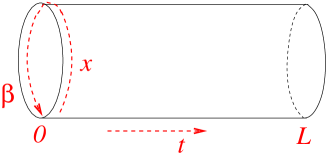
Figure 3: Closed string worldsheet

In the latter, a collection of $N$ closed strings of length $\beta$, is described by fields $\,g_{i}(t,x)={\rm e}^{{\rm i}\varphi_{i}(x,t)}\,$ defined for real $\,t\,$ and $\,x\,$ and twisted-periodic in the $\,x\,$ direction:

$$g_{i}(t,x+\beta)=g_{i}(t,x)\,{\rm e}^{-\beta V}\,,$$ (7.1)

where $\,V\,$ is taken imaginary, compare to (6.15). On the classical level and for Minkowski time, such fields are governed by the action functional

$$S[\bm{g}]=\frac{{}_{1}}{{}^{4\pi}}\sum\limits_{i=1}^{N}\int{\rm d}t\int\limits_{0}^{\beta}\,r_{i}^{2}\big{(}(\partial_{t}\varphi_{i})^{2}-(\partial_{x}\varphi_{i})^{2}\big{)}\,{\rm d}x\,.$$ (7.2)

The twist in the periodicity condition may be absorbed by setting

$$\varphi_{i}(t,x)\equiv\hat{\varphi}_{i}(t,x)+{\rm i}Vx\,,$$ (7.3)

where

$$\hat{\varphi}_{i}(t,x+\beta)=\hat{\varphi}_{i}(t,x)+2\pi m_{i},\qquad m_{i}\in\mathbb{Z}\,.$$ (7.4)

The classical solutions have the form

$$\hat{\varphi}_{i}(t,x)=\hat{\varphi}_{i}^{\ell}(t+x)+\hat{\varphi}_{i}^{r}(t-x)\,,$$ (7.5)

where

$$\hat{\bm{\varphi}}^{\ell,r}(t\pm x)\,=\,\hat{\bm{\varphi}}^{\ell,r}_{0}+\frac{{}_{\sqrt{2}\,\pi}}{{}^{\beta}}\bm{\alpha}_{0}^{\ell,r}(t\pm x)+\frac{{}_{{\rm i}}}{{}^{\sqrt{2}\,}}\sum\limits_{n\not=0}\frac{{}_{1}}{{}^{n}}\bm{\alpha}^{\ell,r}_{n}{\rm e}^{-\frac{2\pi{\rm i}n(t\pm x)}{\beta}}$$ (7.6)

for $\,\overline{\bm{\alpha}^{\ell,r}_{n}}=\bm{\alpha}^{\ell,r}_{-n}$, $\,\,\hat{\varphi}_{0}^{\ell}+\hat{\varphi}_{0}^{r}\equiv\hat{\varphi}_{0}\in(\mathbb{R}/2\pi\mathbb{Z})^{N}$, $\,\frac{1}{\sqrt{2}}(\bm{\alpha}_{0}^{\ell}+\bm{\alpha}_{0}^{r})\equiv\bm{p}_{0}\in{\mathbb{R}}^{N}$,  and

$$\frac{{}_{1}}{{}^{\sqrt{2}}}(\bm{\alpha}_{0}^{\ell}-\bm{\alpha}_{0}^{r})=\bm{m}$$ (7.7)

where $\bm{m}$ is the vector of $N$ winding numbers $m_{i}\in\mathbb{Z}$. The symplectic form on the space of classical solutions is

$$\Omega\,=\, \bm{\delta}p_{0}\cdot\wedge\delta\hat{\bm{\varphi}}_{0}-\frac{{}_{\rm i}}{{}^{2}}\sum_{n\neq 0}\frac{{}_{1}}{{}^{n}}\delta\bm{\alpha}_{n}^{\ell}\cdot\wedge\bm{\alpha}_{(-n)}^{\ell}-\frac{{}_{\rm i}}{{}^{2}}\sum_{n\neq 0}\frac{{}_{1}}{{}^{n}}\delta\bm{\alpha}_{n}^{r}\cdot\wedge\bm{\alpha}_{(-n)}^{r}\,.$$ (7.8)

7.2 Quantization

The Poisson brackets obtained from $\Omega$ lead to the following canonical commutators:

$$\big{[}\varphi_{0i},p_{0j}\big{]}={\rm i}r_{i}^{-2}\delta_{ij}\,,\quad\big{[}\alpha_{ni}^{\ell},\alpha_{n^{\prime}j}^{\ell}\big{]}=r_{i}^{-2}\delta_{ij}\,n\,\delta_{n+n^{\prime},0}\,,\quad\big{[}\alpha_{ni}^{r},\alpha_{n^{\prime}j}^{r}\big{]}=r_{i}^{-2}\delta_{ij}\,n\,\delta_{n+n^{\prime},0}\,.$$ (7.9)

For fixed winding numbers, the zero modes will be represented in the Hilbert space $\,L^{2}\big{(}U(1)^{N}\big{)}\,$ with an orthonormal-basis vectors

$$\left|\bm{k}\right\rangle\equiv\left|k^{1}\ldots k^{N}\right\rangle=\,\exp\Big{(}{\rm i}\sum_{i=1}^{N}k^{i}\varphi_{0i}\Big{)}\qquad\text{for }\ k^{i}\in\mathbb{Z}$$ (7.10)

such that

$$r_{i}^{2}p_{0i}\left|\bm{k}\right\rangle\equiv-{\rm i}\,\frac{{}_{\partial\,\,}}{{}^{\partial\varphi_{0i}}}\,\exp\Big{(}{\rm i}\sum_{i^{\prime}=1}^{N}k^{i^{\prime}}\varphi_{0i^{\prime}}\Big{)}=\,k^{i}\left|\bm{k}\right\rangle.$$ (7.11)

The Hilbert space of states for the zero modes is a direct sum of an infinite number of copies of $\,L^{2}\big{(}U(1)^{N}\big{)}$,  one for each winding vector,

$$\mathcal{H}_{0}\,=\mathop{\oplus}\limits_{\bm{m}\in\mathbb{Z}^{N}}L^{2}\big{(}U(1)^{N}\big{)}\,,$$ (7.12)

with an orthonormal-basis vectors $\left|\bm{k},\bm{m}\right\rangle$. The non-zero modes are represented in the tensor product of two standard Fock spaces ${\mathcal{F}}^{\ell,r}$ generated by applying products of the $\alpha_{ni}^{\ell,r}$ with negative $n$ to the normalized vectors $|0\rangle^{\ell,r}$, annihilated by $\alpha_{ni}^{\ell,r}$ with positive $n$. The scalar products are defined by demanding that $(\alpha_{ni}^{\ell,r})^{\dagger}=\alpha_{(-n)i}^{\ell,r}$. The Hilbert space of the full theory is

$$\mathcal{H}=\mathcal{H}_{0}\otimes{\mathcal{F}}^{\ell}\otimes{\mathcal{F}}^{r}$$ (7.13)

and we identify $\left|\bm{k},\bm{m}\right\rangle\equiv\left|\bm{k},\bm{m}\right\rangle\otimes\left|0\right\rangle^{\ell}\otimes\left|0\right\rangle^{r}$.

7.3 Current, energy and (magnetic) charge

As before, we define the left and right current for the closed string

$${\cal J}_{i}^{\ell,r}(t,x)=\frac{{}_{r_{i}^{2}}}{{}^{2\pi}}\frac{{}_{1}}{{}^{2}}(\partial_{t}\pm\partial_{x})\varphi_{i}(t,x)=\frac{{}_{r_{i}^{2}}}{{}^{\sqrt{2}\,\beta}}\sum_{n}\alpha_{ni}^{\ell,r}\,{\rm e}^{-\frac{2\pi{\rm i}n(t\pm x)}{\beta}}\pm\frac{{}_{{\rm i}r_{i}^{2}V}}{{}^{4\pi}}\,.$$ (7.14)

The classical Hamiltonian of the system is

$$H=\frac{{}_{1}}{{}^{4\pi}}\sum_{i}\int\limits_{0}^{\beta}r_{i}^{2}\Big{(}(\partial_{t}\hat{\varphi}_{i})^{2}+(\partial_{x}\hat{\varphi}_{i})^{2}+2{\rm i}V\partial_{x}\hat{\varphi}_{i}-V^{2}\Big{)}\,{\rm d}x\,.$$ (7.15)

Once quantized, its $\,V$-independent part becomes the standard Hamiltonian of $N$ closed strings

$$\frac{{}_{2\pi}}{{}^{\beta}}\sum_{i}\big{(}L^{\ell}_{0i}+L_{0i}^{r}-\frac{{}_{1}}{{}^{12}}\big{)}\,\equiv\,H_{\rm cs}\,,$$ (7.16)

where

$$L^{\ell,r}_{0i}=\frac{{}_{r_{i}^{2}}}{{}^{2}}\sum\limits_{n}:\alpha^{\ell,r}_{ni}\alpha^{\ell,r}_{-ni}:$$ (7.17)

and the $-\frac{1}{12}$ term comes from the zero-point energy. In the action on $\,{\cal H}_{0}\,$ vectors,

$$H_{\rm cs}\left|\bm{k},\bm{m}\right\rangle=\frac{{}_{\pi}}{{}^{\beta}}\Big{(}\sum_{i}(r_{i}^{-2}(k^{i})^{2}+r_{i}^{2}m_{i}^{2})\,-\frac{{}_{N}}{{}^{6}}\Big{)}\left|\bm{k},\bm{m}\right\rangle\,.$$ (7.18)

The action of excited mode operators $\alpha_{(-n)i}^{\ell,r}$ for positive $n$ raises the eigenvalue of $H_{\rm cs}$ by $\frac{2\pi n}{\beta}$.  The part of the Hamiltonian linear in $\,V\,$ is equal to $\,{\rm i}V\,Q^{m}_{cs}$,  where

$$Q^{\rm m}_{\rm cs}=\sum_{i}\int_{0}^{\beta}\big{(}\hat{\mathcal{J}}_{i}^{\ell}(x,t)-\hat{\mathcal{J}}_{i}^{r}(x,t)\big{)}\,{\rm d}x=\frac{{}_{1}}{{}^{\sqrt{2}}}\sum_{i}r_{i}^{2}(\alpha_{0i}^{\ell}-\alpha_{0i}^{r})\,.$$ (7.19)

is the total magnetic charge of the closed (untwisted) strings. It acts only on $\mathcal{H}_{0}$:

$$Q_{\rm cs}^{\rm m}\,\left|\bm{k},\bm{m}\right\rangle=\sum_{i}r_{i}^{2}m_{i}\left|\bm{k},\bm{m}\right\rangle.$$ (7.20)

Finally, the part of the Hamiltonian quadratic in $\,V\,$ is an additive constant, so that the full quantum Hamiltonian of the closed-string system becomes

$$H\,\equiv\,H_{\rm cs}+{\rm i}V\,Q^{\rm m}_{\rm cs}-\frac{{}_{V^{2}\beta}}{{}^{4\pi}}\sum_{i}r_{i}^{2}.$$ (7.21)

7.4 Boundary states

In the closed-string pictures, the boundary conditions in the space direction, which in that picture becomes the time direction, are represented by the boundary states in the (completion of) the closed-string space of states [38, 21]. The boundary state that corresponds to Neumann boundary condition for all field component is

$$\left|\left|{\cal N}\right\rangle\right\rangle=A_{\cal N}\sum_{\bm{m}\in\mathbb{Z}^{N}}{\rm e}^{-\sum\limits_{n=1}^{\infty}\frac{1}{n}\bm{\alpha}^{\ell}_{-n}\cdot\hskip 0.85355pt\bm{\alpha}_{-n}^{r}}\,\left|\bm{0},\bm{m}\right\rangle\,,$$ (7.22)

where $A_{N}$ is a suitable normalization constant. This boundary state satisfies the relation

$$\partial_{t}\varphi_{i}(0,x)\left|\left|{\cal N}\right\rangle\right\rangle=0\,$$ (7.23)

whose excited-mode part implies that

$$(\alpha_{ni}^{\ell}+\alpha_{(-n)i}^{r})\left|\left|{\cal N}\right\rangle\right\rangle=0$$ (7.24)

determining the form of the Ishibashi-type dependence of $\left|\left|{\cal N}\right\rangle\right\rangle$ on those modes. For the mixed Dirichlet-Neumann boundary condition describing the junction of wires, the boundary state has a more complicated form

$$\left|\left|{\cal B}\right\rangle\right\rangle=A_{DN}\,(2\pi)^{M-N}\sqrt{\det T}$$ (7.25)

$$\times\sum_{\begin{subarray}{c}\bm{k}\in\mathbb{Z}^{N}\\ \sum_{i}k^{i}\kappa_{i}^{m}=0\end{subarray}}\ \sum_{\begin{subarray}{c}\bm{m}\in\mathbb{Z}^{N}\\ m_{i}=\sum_{i}\kappa_{i}^{m}s_{m}\end{subarray}}{\rm e}^{-\sum\limits_{j=1}^{M}\sum\limits_{n=1}^{\infty}\frac{1}{n}\tilde{\alpha}_{(-n)j}^{\ell}\tilde{\alpha}_{(-n)j}^{r}\,+\sum\limits_{j=M+1}^{N}\sum\limits_{n=1}^{\infty}\frac{1}{n}\tilde{\alpha}_{(-n)j}^{\ell}\tilde{\alpha}_{(-n)j}^{r}}\,\left|\bm{k},\bm{m}\right\rangle,\qquad$$ (7.26)

where $s_{m}$ run through integers and $\,\tilde{\alpha}_{nj}^{\ell,r}=\bm{\Lambda}_{j}\cdot\bm{\alpha}^{\ell,r}_{n}$,  see (4.9).  One has

$$P\hskip 0.85355pt\partial_{t}\bm{\varphi}(0,x)\left|\left|{\cal B}\right\rangle\right\rangle=0,\qquad(1-P)\hskip 0.56917pt\bm{\varphi}(0,x)\left|\left|{\cal B}\right\rangle\right\rangle=0\,,$$ (7.27)

where field $\,\bm{\varphi}\,$ may be equivalently replaced by $\,\hat{\bm{\varphi}}$.  The excited-mode part of these conditions implies that

$$(\tilde{\alpha}_{nj}^{\ell}+\tilde{\alpha}_{(-n)j}^{r})\left|\left|{\cal B}\right\rangle\right\rangle=0\quad\text{for}\quad j\leq M\,,\qquad(\tilde{\alpha}_{nj}^{\ell}-\tilde{\alpha}_{(-n)j}^{r})\left|\left|{\cal B}\right\rangle\right\rangle=0\quad\text{for}\quad j>M\,,$$ (7.28)

fixing the form of the Ishibashi building-blocks of $\,\left|\left|{\cal B}\right\rangle\right\rangle$. The zero-mode part of the first of relations (7.27) assures that $\sum\limits_{i}k^{i}\kappa^{m}_{i}=0$, whereas the zero-mode part of the second relations implies that $(1-P)\bm{m}=0$ which is solved by $m_{i}=\sum\limits_{m}\kappa^{m}_{i}s_{m}$ for integer $s_{m}$. The sum

$$(2\pi)^{M-N}\,\sqrt{\det T}\sum_{\begin{subarray}{c}\bm{k}\in\mathbb{Z}^{N}\\ \sum_{i}k^{i}\kappa_{i}^{m}=0\end{subarray}}\left|\bm{k}\right\rangle$$ (7.29)

represents the delta-function supported by the brane ${\cal B}=\kappa(U(1)^{M})\subset U(1)^{N}$ defined by the integral

$$\delta_{B}(\varphi_{0})\equiv\int\prod_{i}\delta\big{(}\varphi_{0i}-\sum_{m}\kappa_{i}^{m}\psi_{m})\,\sqrt{\det T}\,\prod_{m}{\rm d}\psi_{m}$$ (7.30)

over $\,U(1)^{M}$ of  the $\,2\pi-$periodic $\,N$-dimensional $\,\delta$-function. Indeed,

$$\delta_{B}(\varphi_{0}) =\sqrt{\det T}\,\int\frac{{}_{1}}{{}^{(2\pi)^{N}}}\sum_{\bm{k}\in\mathbb{Z}^{N}}{\rm e}^{i\sum_{i}k^{i}(\varphi_{0i}-\sum_{m}\kappa_{i}^{m}\psi_{m})}\prod_{m}{\rm d}\psi_{m}$$ (7.31)

$$=(2\pi)^{M-N}\sqrt{\det T}\,\sum_{\bm{k}\in\mathbb{Z}^{N}}{\rm e}^{i\sum_{i}k^{i}\varphi_{0i}}\delta_{\sum_{i}k^{i}\kappa_{i}^{m},0}$$ (7.32)

which reproduces (7.29).

7.5 Partition function

In the closed-string picture, the partition function $Z_{\beta,V}$ is represented by the matrix element of the Euclidean evolution operator ${\rm e}^{-LH}$ between the boundary states. A direct calculation gives:

$$Z_{\beta,V} =\left\langle\left\langle{\cal N}\right|\right|{\rm e}^{-LH}\left|\left|{\cal B}\right\rangle\right\rangle$$ (7.33)

$$=A_{N}A_{B}(2\pi)^{M-N}\sqrt{\det T}\,\left[\eta\big{(}\frac{{}_{2{\rm i}L}}{{}^{\beta}}\big{)}\right]^{N-2M}\left[\eta\big{(}\frac{{}_{4{\rm i}L}}{{}^{\beta}}\big{)}\right]^{M-N}\,{\rm e}^{\frac{{}_{NV^{2}\beta L}}{{}^{4\pi}}\sum_{i}r_{i}^{2}}$$ (7.34)

$$\times\sum_{\begin{subarray}{c}\bm{m}\in\mathbb{Z}^{N}\\ m_{i}=\sum\kappa_{i}^{m}s_{m}\end{subarray}}{\rm e}^{-\frac{\pi L}{\beta}\sum(r_{i}m_{i})^{2}-{\rm i}LV\sum r_{i}^{2}m_{i}}\,.$$ (7.35)

This coincides with expression (5.5) upon relabeling $\bm{s}=\bm{k}$ and recalling the definition (4.44) of vector $\,\bm{p}$,  provided that

$$A_{N}A_{B}(2\pi)^{M-N}=\,2^{-N}\,.$$ (7.36)

The latter identity is assured if we take $A_{N}=A^{N}$ and $A_{B}=A^{M}B^{N-M}$ for $A=\frac{1}{\sqrt{2}}$ and $B=\sqrt{2}\pi$.

7.6 Expectations

The expectation values of products of currents in equilibrium state $\,\omega^{L}_{\beta,V}$ take in the open string picture the form of the matrix elements between the boundary states of the time ordered products of Euclidean versions of currents ${\cal J}^{\ell,r}$:

$$\omega^{L}_{\beta,V}\Big{(}\prod\limits_{k=1}^{K}J_{i_{k}}^{\ell}(0,x_{k})\prod\limits_{k^{\prime}=1}^{K^{\prime}}J_{i_{k^{\prime}}}^{r}(0,y_{k^{\prime}})\Big{)}= \,\frac{(-{\rm i})^{K}{\rm i}^{K^{\prime}}}{\left\langle\left\langle{\cal N}\right|\right|{\rm e}^{-LH}\left|\left|{\cal B}\right\rangle\right\rangle}$$ (7.37)

$$\times\ \left\langle\left\langle{\cal N}\right|\right|{\rm e}^{-LH}\,{\cal T}\prod\limits_{k=1}^{K}{\cal J}_{i_{k}}^{\ell}(-{\rm i}x_{k},0)\prod\limits_{k^{\prime}=1}^{K^{\prime}}{\cal J}_{i_{k^{\prime}}}^{r}(-{\rm i}y_{k^{\prime}},0)\left|\left|{\cal B}\right\rangle\right\rangle,$$ (7.38)

where the Euclidean time ordering puts the operators at bigger $\,x_{k}\,$ or $\,y_{k^{\prime}}\,$ to the left. The powers of $\,-{\rm i}\,$ and $\,{\rm i}\,$ represent the derivatives of the Euclidean conformal change of variables, $\,x+{\rm i}t\mapsto t-{\rm i}x\,$ and $\,y-{\rm i}t\mapsto t+{\rm i}y$,  respectively,  that reverses the roles of time and space.

The proof of (7.37) in done in few steps. First, consider only the left currents. As in the initial picture,  we distinguish the constant part from the excited terms,

$${\cal J}_{i}^{\ell}(t,x)=\frac{{}_{{\rm i}r_{i}^{2}V}}{{}^{4\pi}}+\frac{{}_{r_{i}^{2}}}{{}^{\sqrt{2}\,\beta}}\alpha_{0i}^{\ell}+\hat{\cal J}_{i}^{\ell}(t,x)\,,$$ (7.39)

see (7.14). This decomposition factorizes in the expectation values. For the constant terms, we get by direct calculation:

$$(-{\rm i})^{K}Z_{\beta,V}^{-1}\left\langle\left\langle{\cal N}\right|\right|{\rm e}^{-LH}\prod_{k=1}^{K}\Big{(}\frac{{}_{{\rm i}r_{i_{k}}^{2}V}}{{}^{4\pi}}+\frac{{}_{r_{i_{k}}^{2}}}{{}^{\sqrt{2}\,\beta}}\alpha_{0i_{k}}^{\ell}\Big{)}\left|\left|{\cal B}\right\rangle\right\rangle$$ (7.40)

$$=\frac{{}_{1}}{{}^{(2\beta VL)^{K}}}\prod_{k=1}^{K}r_{i_{k}}^{2}\sum\limits_{m}\kappa^{m}_{i_{k}}\Big{(}\dfrac{\frac{\partial}{\partial p^{m}}{\rm e}^{\frac{L\beta V^{2}}{4\pi}\bm{p}\cdot T^{-1}\bm{p}}}{{\rm e}^{\frac{L\beta V^{2}}{4\pi}\bm{p}\cdot T^{-1}\bm{p}}}+\,\dfrac{\frac{\partial}{\partial p^{m}}\Big{(}\sum\limits_{\bm{k}\in\mathbb{Z}^{M}}{\rm e}^{-{\rm i}LV\bm{p}\cdot\bm{k}-\frac{\pi L}{\beta}\bm{k}\cdot T\bm{k}}\Big{)}}{\sum\limits_{\bm{k}\in\mathbb{Z}^{M}}{\rm e}^{-{\rm i}LV\bm{p}\cdot\bm{k}-\frac{\pi L}{\beta}\bm{k}\cdot T\bm{k}}}\Big{)}$$ (7.41)

$$=\omega^{L}_{\beta,V}\Big{(}\prod_{k=1}^{K}\big{(}J^{\ell}_{i_{k}}(t,x)-\hat{J}^{\ell}_{i_{k}}(t,x)\big{)}\Big{)}-\sum_{\{\ldots(k_{p},l_{p})\ldots\}}\prod_{p}\frac{{}_{r^{2}_{i_{k_{p}}}}}{{}^{8\pi L\beta}}P_{i_{k_{p}}i_{l_{p}}}\,,$$ (7.42)

which almost reproduces the zero mode part expectation value (5.9) of the initial calculation but with one extra term, where $\{\ldots(k_{p},l_{p})\ldots\}$ runs through all possible pairing of $\{1,\ldots,K\}$, as in the Wick theorem. The presence of this term can be seen by induction on $K$. On the other hand, the expectations of products of $\hat{\cal J}^{\ell}_{i}$ are calculated by the Wick rule with

$$-{\rm i}Z_{\beta,V}^{-1}\left\langle\left\langle{\cal N}\right|\right|{\rm e}^{-LH}\hat{\cal J}^{\ell}_{i}(-{\rm i}x,0)\left|\left|{\cal B}\right\rangle\right\rangle=0\,,$$ (7.43)

$$(-{\rm i})^{2}Z_{\beta,V}^{-1}\left\langle\left\langle{\cal N}\right|\right|{\rm e}^{-LH}\hat{\cal J}^{\ell}_{i_{1}}(-{\rm i}x_{1},0)\hat{\cal J}^{\ell}_{i_{2}}(-{\rm i}x_{2},0)\left|\left|{\cal B}\right\rangle\right\rangle$$ (7.44)

$$\hskip 56.9055pt=-\frac{{}_{1}}{{}^{2}}\left(\frac{{}_{r_{i_{1}}}}{{}^{2\pi}}\right)^{2}\Big{(}P_{i_{1}i_{2}}\,(\wp(x_{1}-x_{2};2L,-{\rm i}\beta)+C_{e}^{\prime})$$ (7.45)

$$\hskip 68.28644pt+(\delta_{i_{1}i_{2}}-P_{i_{1}i_{2}})(2{\wp}(x_{1}-x_{2};4L,-{\rm i}\beta)-{\wp}(x_{1}-x_{2};2L,-{\rm i}\beta)+C_{o}^{\prime})\Big{)},\quad\quad$$ (7.46)

where we get expressions with the Weierstrass function similar to (5.11) but with different constants

$$C_{e}^{\prime}= \left(\frac{{}_{\pi}}{{}^{-{\rm i}\beta}}\right)^{2}\Big{(}\frac{{}_{1}}{{}^{3}}-\sum_{p\neq 0}\big{(}\sinh(\pi\frac{{}_{2Lp}}{{}^{\beta}})\big{)}^{-2}\Big{)},$$ (7.47)

$$C_{o}^{\prime}= \left(\frac{{}_{\pi}}{{}^{-{\rm i}\beta}}\right)^{2}\Big{(}\frac{{}_{1}}{{}^{3}}-2\sum_{p\neq 0}\big{[}\sinh\big{(}\pi\frac{{}_{4Lp}}{{}^{\beta}}\big{)}\big{]}^{-2}+\sum_{p\neq 0}\big{[}\sinh\big{(}\pi\frac{{}_{2Lp}}{{}^{\beta}}\big{)}\big{]}^{-2}\Big{)}.$$ (7.48)

The theory of Weierstrass function of periods $\omega_{1}$ and $\omega_{2}$ [47] provides the identity

$$\frac{{}_{\omega_{1}}}{{}^{\omega_{2}}}\Big{(}\frac{{}_{1}}{{}^{3}}+\sum_{n\neq 0}\sin^{-2}\big{(}\frac{{}_{\pi n\omega_{1}}}{{}^{\omega_{2}}}\big{)}\Big{)}-\frac{{}_{\omega_{2}}}{{}^{\omega_{1}}}\Big{(}\frac{{}_{1}}{{}^{3}}+\sum_{n\neq 0}\sin^{-2}\big{(}\frac{{}_{\pi n\omega_{2}}}{{}^{\omega_{1}}}\big{)}\Big{)}=\pm\frac{{}_{{\rm i}}}{{}^{\pi}}\,,$$ (7.49)

where the sign on the right hand side is that of the imaginary part of $\omega_{1}/\omega_{2}$. This leads to the relations

$$C_{o}^{\prime}=C_{o}\,,\qquad C_{e}^{\prime}=C_{e}-\frac{{}_{\pi}}{{}^{L\beta}}\,.$$ (7.50)

The contribution from the last term will cancel exactly the last contribution appearing in (7.40) establishing identity (7.37) for any product of left currents. Finally, the closed-string expectation value of a general product of left and right current will be a combination of factors corresponding to the decomposition (7.14). By direct calculation, the constant part of the right currents can be expressed via the $S$ matrix in terms of the one of the left currents with the use of (4.26) and the fact that $S$ also preserves vectors $\,\bm{\kappa}^{m}$.  In the computation of the excited part, the $S$ matrix appears naturally upon noticing that in the proper basis defined in (4.9), it becomes

$$\tilde{S}=\text{diag}(\underbrace{1,\ldots,1}_{M},-1,\ldots,-1)$$ (7.51)

which is precisely how the excited modes $\tilde{\alpha}_{ni}^{\ell}$ and $\tilde{\alpha}_{ni}^{r}$ are related when they act on $\left|\left|{\cal B}\right\rangle\right\rangle$, see (7.28). Finally, under the closed-string expectation every right current is related to the left one by the $S$ matrix, exactly as in the initial picture (4.30). This proves identity (7.37) in the general case.

8 Thermodynamic limit

In the thermodynamic limit $L\to\infty$ the wires become infinitely long. The partition function $Z_{\beta,V}$ diverges in that situation but the free energy per unit length has a limit:

$$f^{L}_{\beta,V}\,=\,-\frac{{}_{1}}{{}^{L\beta}}\ln{Z_{\beta,V}}\ \,\mathop{\longrightarrow}\limits_{L\to\infty}\ \,-\frac{{}_{V^{2}}}{{}^{4\pi}}\sum\limits_{i=1}^{N}r_{i}^{2}\,-\frac{{}_{\pi N}}{{}^{6\beta^{2}}}\ \equiv\ f_{\beta,V}\,,$$ (8.1)

as easily follows from its form (5.5). The equilibrium state expectation values of the products of currents also possess the $L\to\infty$ limit. In particular, it follows from (5.9) that

$$\lim\limits_{L\to\infty}\,\omega^{L}_{\beta,V}\Big{(}\prod\limits_{k=1}^{K}\frac{{}_{r_{i_{k}}^{2}}}{{}^{4L}}\,\alpha_{0i_{k}}^{\ell}\Big{)}\ =\ \prod\limits_{k=1}^{K}\frac{{}_{r_{i_{k}}^{2}V}}{{}^{4\pi}}$$ (8.2)

for real $\,V\,$ and relations (5.10) and (5.11) imply that

$$\lim\limits_{L\to\infty}\,\omega^{L}_{\beta,V}\big{(}\hat{J}^{\ell}_{i}(t,x)\big{)}\ =\ 0\,,$$ (8.3)

$$\lim\limits_{L\to\infty}\,\omega^{L}_{\beta,V}\big{(}\hat{J}^{\ell}_{i_{1}}(t,x_{1})\,\hat{J}^{\ell}_{i_{2}}(t,x_{2})\big{)}\ =\ -\,\delta_{i_{1}i_{2}}\,\frac{{}_{r_{i_{1}}^{2}}}{{}^{8\beta^{2}}}\,\sinh^{-2}\left(\frac{{}_{\pi(x_{1}-x_{2})}}{{}^{\beta}}\right),$$ (8.4)

as both $\,f_{e}(x)\,$ and $\,f_{o}(x)\,$ tend to $\,\big{(}\frac{\pi}{\beta}\big{)}^{2}\,\sinh^{-2}\big{(}\frac{\pi x}{\beta}\big{)}\,$ when $\,L\to\infty$. The latter property follows from (5.17) and the identity (7.49). Eqs. (8.2), (5.10), (8.4) and the Wick rule, as well as the relation (4.30), determine the $L\to\infty$ limit $\,\omega_{\beta,V}$ of the states $\,\omega^{L}_{\beta,V}$. Unlike for finite $L$, that limit is not represented by a trace with a density matrix (for $L=\infty$, the Hamiltonian has a continuous spectrum and the operator ${\rm e}^{-\beta(H-VQ)}$ is not traceclass). In particular, one obtains:

$$\omega_{\beta,V}\big{(}J^{\ell}_{i}(t,x)\big{)}\,=\,\frac{{}_{r_{i}^{2}V}}{{}^{4\pi}}\,,$$ (8.5)

$$\omega_{\beta,V}\big{(}J^{\ell}_{i_{1}}(t,x_{1})\,J^{\ell}_{i_{2}}(t,x_{2})\big{)}\,=\,\frac{{}_{r_{i_{1}}^{2}r_{i_{2}}^{2}V^{2}}}{{}^{16\pi^{2}}}\,-\,\delta_{i_{1}i_{2}}\,\frac{{}_{r_{i_{1}}^{2}}}{{}^{8\beta^{2}}}\,\sinh^{-2}\left(\frac{{}_{\pi(x_{1}-x_{2})}}{{}^{\beta}}\right).$$ (8.6)

The operator product expressions (5.23) and the limit (8.4) (that is uniform in small $|x_{1}-x_{2}|$) imply that

$$\omega_{\beta,V}\big{(}T^{\ell}_{i}(t,x)\big{)} =\frac{{}_{r_{i}^{2}V^{2}}}{{}^{8\pi}}\,+\,\lim\limits_{\epsilon\to 0}\,\Big{(}-\frac{{}_{\pi}}{{}^{4\beta^{2}}}\sinh^{-2}\big{(}\frac{{}_{\pi\epsilon}}{{}^{\beta}}\big{)}+\frac{{}_{1}}{{}^{4\pi\epsilon^{2}}}\Big{)}=\frac{{}_{r_{i}^{2}V^{2}}}{{}^{8\pi}}+\frac{{}_{\pi}}{{}^{12\beta^{2}}}$$ (8.7)

$$=\,\omega_{\beta,V}\big{(}T^{r}_{i}(t,x)\big{)}.$$ (8.8)

In particular, the mean energy density in the equilibrium state is constant in each semi-infinite wire (but differs from one wire to another) and the mean energy current vanishes.

The $L=\infty$ state is easy to represent in the closed-string picture: by examining the right hand side of (7.37), one infers that the boundary state $\left|\left|{\cal N}\right\rangle\right\rangle$ of (7.22) is projected when $L\to\infty$ to the closed-string vacuum $\left|\bm{0},\bm{0}\right\rangle\,$so that

$$\omega_{\beta,V}\Big{(}\prod\limits_{k=1}^{K}J_{i_{k}}^{\ell}(0,x_{k})\prod\limits_{k^{\prime}=1}^{K^{\prime}}J_{i_{k^{\prime}}}^{r}(0,y_{k^{\prime}})\Big{)}\ =\ \frac{(-{\rm i})^{K}{\rm i}^{K^{\prime}}}{\langle\bm{0},\bm{0}\left|\left|{\cal B}\right\rangle\right\rangle}$$ (8.9)

$$\times\ \left\langle\bm{0},\bm{0}\right|\,{\cal T}\prod\limits_{k}{\cal J}_{i_{k}}^{\ell}(-ix_{k},0)\prod\limits_{k^{\prime}}{\cal J}_{i_{k^{\prime}}}^{r}(-iy_{k^{\prime}},0)\left|\left|{\cal B}\right\rangle\right\rangle$$ (8.10)

for $x_{k},y_{k^{\prime}}>0$,

One of the crucial observations that follows from (8.2) and (8.4) is that, when restricted to the products of left-moving currents $\,J^{\ell}_{i}(0,x)\,$ with $\,x>0$,  the limiting $\,L=\infty\,$ equilibrium expectations do not depend on the choice of the brane $\,{\cal B}\,$ describing the contact of wires. In particular, such expectations are the same as for the space-filling brane $\,{\cal B}_{0}$ with $\,S_{ii^{\prime}}=\delta_{ii^{\prime}}\,$ corresponding to the disconnected wires for which $\,J^{r}_{i}(t,x)=J_{i}^{\ell}(t,-x)\,$ and $\,\left|\left|{\cal B}_{0}\right\rangle\right\rangle=\left|\left|{\cal N}\right\rangle\right\rangle$.  The physical reason for this behavior of the expectations of left-moving currents is that the latter did not have contact with the junction up to time zero. The above observation is essential for the construction of nonequilibrium stationary state where the individual wires are kept at different temperatures and at different potentials. For the disconnected wires, one has the obvious factorization:

$$\omega^{L}_{\beta,V}\Big{(}\prod\limits_{k=1}^{K}J^{\ell}_{i_{k}}(t,x_{k})\Big{)}\,=\,\prod\limits_{i=1}^{N}\,\omega^{L}_{\beta,V}\Big{(}\prod\limits_{\begin{subarray}{c}k\\ i_{k}=i\end{subarray}}J^{\ell}_{i}(t,x_{k})\Big{)}\,.$$ (8.11)

Hence the same formula holds in the $L\to\infty$ limit of the equilibrium state for any brane ${\cal B}=\kappa(U(1)^{M})$.

For the disconnected wires,  one also has the relation:

$$\omega^{L}_{\beta,V}\Big{(}\prod\limits_{{k^{\prime}}=1}^{K^{\prime}}J^{r}_{i_{k^{\prime}}}(t,y_{k^{\prime}})\Big{)}\,=\,\prod\limits_{i={k^{\prime}}}^{N}\,\omega^{L}_{\beta,V}\Big{(}\prod\limits_{\begin{subarray}{c}k^{\prime}\\ i_{k^{\prime}}=i\end{subarray}}J^{r}_{i}(t,y_{k^{\prime}})\Big{)}\,=\,\,\prod\limits_{i=1}^{N}\,\omega^{L}_{\beta,V}\Big{(}\prod\limits_{\begin{subarray}{c}k^{\prime}\\ i_{k^{\prime}}=i\end{subarray}}J^{\ell}_{i}(t,-y_{k^{\prime}})\Big{)}.$$ (8.12)

It is easy to check using (4.30) and (4.26) that the latter factorization holds in the limit $L\to\infty$ also for other branes $\,{\cal B}=\kappa(U(1)^{M})$.

9 Nonequilibrium stationary state

Following [32, 11], see also [41], we shall consider a nonequilibrium stationary state (NESS) $\,\omega_{\rm neq}$ describing the situation when different semi-infinite wires are kept at different temperatures and different potentials. State $\,\omega_{\rm neq}$ may be obtained by the following limiting procedure. For each disconnected semi-infinite wire, one considers the algebra $\,{\cal A}_{i}$ generated by products of currents $\,J^{\ell,r}_{i}(0,x)\,$ for $x>0$, together with a state $\,\omega^{i}_{\beta_{i},V_{i}}$ given by the restriction to $\,{\cal A}_{i}$ of the $L=\infty$ equilibrium state $\,\omega_{\beta_{i},V_{i}}$ for the space-filling brane $\,{\cal B}_{0}$. The product state $\,\omega_{\rm in}\equiv\mathop{\otimes}\limits_{i=1}^{N}\omega^{i}_{\beta_{,},V_{i}}$ on algebra $\,{\cal A}=\mathop{\otimes_{i}}{\cal A}_{i}$ describes the disconnected wires with each prepared in its own equilibrium state $\,\omega^{i}_{\beta_{i},V_{i}}$.  As in Sec. 4, algebra $\,{\cal A}\,$ may be identified with the one generated by currents $J^{\ell,r}_{i}(0,x)$ with $x>0$ and $\,1\leq i\leq N\,$ for the connected wires. Let $\,{\cal U}_{t}\,$ for $t>0$ describe the forward in time Heisenberg-picture evolution of the currents $J^{\ell,r}_{i}(0,x)$ with $x>0$ in the presence of brane $\,{\cal B}\,$:

$${\cal U}_{t}J_{i}^{\ell}(0,x)=J^{\ell}_{i}(t,x)=J^{\ell}_{i}(0,x+t)=J_{i}^{\ell}(0,t+x)\,,$$ (9.1)

$${\cal U}_{t}J_{i}^{r}(0,x)=J^{r}_{i}(t,x)=J^{r}_{i}(0,x-t))=\begin{cases}\,J_{i}^{r}(0,x-t)\hskip 38.12659pt{\rm for}\quad t\leq x\cr\,\sum\limits_{i^{\prime}}S_{ii^{\prime}}J^{\ell}_{i^{\prime}}(0,t-x)\hskip 10.81218pt{\rm for}\quad x\leq t\end{cases}$$ (9.2)

Then for $A\in{\cal A}$,

$$\omega_{\rm neq}(A)\,=\,\lim\limits_{t\to\infty}\,\omega_{\rm in}({\cal U}_{t}A)\,.$$ (9.3)

In order to prove the above relation consider the backward in time Heisenberg evolution for decoupled wires, i.e. in the presence of brane ${\cal B}_{0}$:

$$\hskip 28.45274pt{\cal U}^{0}_{-t}J^{\ell}_{i}(0,x)=J^{\ell}_{i}(-t,x)=J^{\ell}_{i}(0,x-t)=\begin{cases}\,J_{i}^{\ell}(0,-t+x)\hskip 26.46085pt{\rm for}\quad t\leq x\,,\cr\,J^{r}_{i}(0,t-x)\hskip 33.57404pt{\rm for}\quad x\leq t\,,\end{cases}$$ (9.4)

$$\hskip 28.45274pt{\cal U}^{0}_{-t}J_{i}^{r}(0,x)=J^{r}_{i}(-t,x)=J^{r}_{i}(0,x+t)=J_{i}^{r}(0,t+x)$$ (9.5)

for $\,x,t>0$.  Such a decoupled evolution preserves the product state $\,\omega_{\rm in}\,$ so that

$$\lim\limits_{t\to\infty}\,\omega_{\rm in}({\cal U}_{t}A)\,=\,\omega_{\rm in}({\cal S}A)\,,$$ (9.6)

where

$${\cal S}=\lim\limits_{t\to\infty}\,{\cal U}^{0}_{-t}{\cal U}_{t}$$ (9.7)

is the scattering operator in the action on algebra $\,{\cal A}$.  The explicit form of the latter in the action on the chiral currents follows from equations (9.1), (9.2), (9.4) and (9.5):

$${\cal S}J^{\ell}_{i}(0,x)\,=\,J^{\ell}_{i}(0,x)\,,$$ (9.8)

$${\cal S}J^{r}_{i}(0,x)\,=\,\sum\limits_{i^{\prime}}S_{ii^{\prime}}J^{r}_{i^{\prime}}(0,x)$$ (9.9)

for $\,x>0$.  Note that the nonequilibrium state $\omega_{\rm neq}$ is preserved by the Heisenberg evolution $\,{\cal U}_{t}\,$  so that its stationarity follows. Hence the explicit formula:

$$\omega_{\rm neq}\bigg{(}\Big{(}\prod\limits_{k=1}^{K}J^{\ell}_{i_{k}}(t,x_{k})\Big{)}\Big{(}\prod\limits_{k^{\prime}=1}^{K^{\prime}}J^{r}_{i_{k^{\prime}}}(t,y_{k^{\prime}})\Big{)}\bigg{)}$$ (9.10)

$$=\,\prod\limits_{k^{\prime}=1}^{K^{\prime}}\sum\limits_{i^{\prime}_{k^{\prime}}}S_{i_{k^{\prime}}i^{\prime}_{k^{\prime}}}\,\prod\limits_{i=1}^{N}\,\omega^{i}_{\beta_{i},V_{i}}\bigg{(}\Big{(}\prod\limits_{\begin{subarray}{c}k\\ i_{k}=i\end{subarray}}J^{\ell}_{i}(t,x_{k})\Big{)}\Big{(}\prod\limits_{\begin{subarray}{c}k^{\prime}\\ i^{\prime}_{k^{\prime}}=i\end{subarray}}J^{r}_{i}(t,y_{k^{\prime}})\Big{)}\bigg{)},$$ (9.11)

where on the left hand side the currents correspond to connected wires and on the right hand side to disconnected ones and the values of $t$, $x_{k}$ and $x_{k^{\prime}}$ may be taken arbitrary (with noncoincident $x_{1},\dots,x_{K},-y_{1},\dots,-y_{K^{\prime}}$ to avoid singularities). In particular,

$$\omega_{\rm neq}\bigg{(}\prod\limits_{k=1}^{K}J^{\ell}_{i_{k}}(t,x_{k})\bigg{)}=\,\omega_{\rm in}\bigg{(}\prod\limits_{k=1}^{K}J^{\ell}_{i_{k}}(t,x_{k})\bigg{)}$$ (9.12)

so that the difference between $\omega_{\rm neq}$ and $\omega_{\rm in}$, due to the junction between wires, arises only in the presence of right-moving currents. The left-moving currents do not feel the influence of the junction. It should be stressed that the dynamics considered above both in the presence of the junction and for decoupled wires is generated by the Hamiltonians that do not include the electric potentials in the bulk of the wires. Those play the role only in the preparation of the initial product state and may be applied far away from the junction. That the ballistic evolution of chiral currents persists for long times in the bulk of the wires in such a nonequilibrium situation should be assured by the integrable nature of the Luttinger liquids, see the discussion at the end of [13].

Specifying Eq. (9.11) to the 1-point expectations, one obtains:

$$\omega_{\rm neq}\big{(}J^{\ell}_{i}(t,x)\big{)}\,=\,\frac{{}_{r_{i}^{2}V_{i}}}{{}^{4\pi}}\,,\qquad\omega_{\rm neq}\big{(}J^{r}_{i}(t,x)\big{)}\,=\,\sum\limits_{i^{\prime}=1}^{N}S_{ii^{\prime}}\frac{{}_{r_{i^{\prime}}^{2}V_{i^{\prime}}}}{{}^{4\pi}}$$ (9.13)

so that the mean charge density and mean current in the wires are

$$\omega_{\rm neq}\big{(}J^{0}_{i}(t,x)\big{)}\,=\,\sum\limits_{i^{\prime}=1}^{N}(S_{ii^{\prime}}+\delta_{ii^{\prime}})\frac{{}_{r_{i^{\prime}}^{2}V_{i^{\prime}}}}{{}^{4\pi}}\,,\qquad\omega_{\rm neq}\big{(}J^{1}_{i}(t,x)\big{)}\,=\,\sum\limits_{i^{\prime}=1}^{N}(S_{ii^{\prime}}-\delta_{ii^{\prime}})\frac{{}_{r_{i^{\prime}}^{2}V_{i^{\prime}}}}{{}^{4\pi}}\,,$$ (9.14)

respectively. They are constant in each wire and the mean current does not vanish, in general, at difference with the equilibrium state. The electric conductance tensor of the junction (in the units $\,e^{2}/\hbar$)  is

$${}^{\rm el}G_{ii^{\prime}}\equiv\left.\frac{{}_{\partial\,}}{{}^{\partial V_{i^{\prime}}}}\,\omega_{\rm neq}(J^{1}_{i}(0,x))\right|_{\begin{subarray}{c}\beta_{j}=\beta\\ V_{j}=V\end{subarray}}=\frac{{}_{1}}{{}^{4\pi}}(S_{ii^{\prime}}-\delta_{ii^{\prime}})r_{i^{\prime}}^{2}\,.$$ (9.15)

This agrees with the calculation of [39, 40] based on the combination of the Green-Kubo formula with the conformal field theory representation of the equilibrium state. Note that the conductance vanishes for the decoupled wires. The nonequilibrium current 2-point functions are given by

$$\omega_{\rm neq}\big{(}J^{\ell}_{i_{1}}(t,x_{1})\,J^{\ell}_{i_{2}}(t,x_{2})\big{)}\,=\,\frac{{}_{r_{i_{1}}^{2}r_{i_{2}}^{2}V_{i_{1}}V_{i_{2}}}}{{}^{16\pi^{2}}}\,-\,\delta_{i_{1}i_{2}}\,\frac{{}_{r_{i_{1}}^{2}}}{{}^{8\beta_{i_{1}}^{2}}}\,\sinh^{-2}\left(\frac{{}_{\pi(x_{1}-x_{2})}}{{}^{\beta_{i_{1}}}}\right),$$ (9.16)

$$\omega_{\rm neq}\big{(}J^{\ell}_{i_{1}}(t,x_{1})\,J^{r}_{i_{2}}(t,x_{2})\big{)}\,=\,\sum\limits_{i=1}^{N}S_{i_{2}i}\frac{{}_{r_{i_{1}}^{2}r_{i}^{2}V_{i_{1}}V_{i}}}{{}^{16\pi^{2}}}\,-\,S_{i_{2}i_{1}}\,\frac{{}_{r_{i_{1}}^{2}}}{{}^{8\beta_{i_{1}}^{2}}}\,\sinh^{-2}\left(\frac{{}_{\pi(x_{1}+x_{2})}}{{}^{\beta_{i_{1}}}}\right),$$ (9.17)

$$\omega_{\rm neq}\big{(}J^{r}_{i_{1}}(t,x_{1})\,J^{r}_{i_{2}}(t,x_{2})\big{)}\,=\sum\limits_{i,i^{\prime}=1}^{N}S_{i_{1}i}S_{i_{2}i^{\prime}}\frac{{}_{r_{i}^{2}r_{i^{\prime}}^{2}V_{i}V_{i^{\prime}}}}{{}^{16\pi^{2}}}-\sum\limits_{i=1}^{N}S_{i_{1}i}S_{i_{2}i}\,\frac{{}_{r_{i}^{2}}}{{}^{8\beta_{i}^{2}}}\,\sinh^{-2}\left(\frac{{}_{\pi(x_{1}-x_{2})}}{{}^{\beta_{i}}}\right).$$ (9.18)

Note that the nonequilibrium states $\,\omega_{\rm neq}$ with coupled wires break the time reversal symmetry $J^{\ell}\leftrightarrow J^{r}$.

For the expectation value of the energy-momentum components, we obtain from the operator product expansions (5.24) and (5.25)

$$\omega_{\rm neq}\big{(}T^{\ell}_{i}(t,x)\big{)}\, =\,\frac{{}_{r_{i}^{2}V_{i}^{2}}}{{}^{8\pi}}\,+\,\lim\limits_{\epsilon\to 0}\Big{(}-\frac{{}_{\pi}}{{}^{4\beta_{i}^{2}}}\sinh^{-2}\Big{(}\frac{{}_{\pi\epsilon}}{{}^{\beta_{i}}}\Big{)}+\frac{{}_{1}}{{}^{4\pi\epsilon^{2}}}\Big{)}\,=\,\frac{{}_{r_{i}^{2}V_{i}^{2}}}{{}^{8\pi}}\,+\,\frac{{}_{\pi}}{{}^{12\beta_{i}^{2}}}\,,$$ (9.19)

$$\omega_{\rm neq}\big{(}T^{r}_{i}(t,x)\big{)}\, =\,\frac{{}_{1}}{{}^{8\pi r_{i}^{2}}}\Big{(}\sum\limits_{i^{\prime}=1}^{N}S_{ii^{\prime}}r_{i^{\prime}}^{2}V_{i^{\prime}}\Big{)}^{2}\,+\,\lim\limits_{\epsilon\to 0}\Big{(}-\sum\limits_{i^{\prime}=1}^{N}(S_{ii^{\prime}})^{2}\frac{{}_{\pi r_{i^{\prime}}^{2}}}{{}^{4r_{i}^{2}\beta_{i^{\prime}}^{2}}}\sinh^{-2}\Big{(}\frac{{}_{\pi\epsilon}}{{}^{\beta_{i^{\prime}}}}\Big{)}+\frac{{}_{1}}{{}^{4\pi\epsilon^{2}}}\Big{)}$$ (9.20)

$$\,=\,\frac{{}_{1}}{{}^{8\pi r_{i}^{2}}}\Big{(}\sum\limits_{i^{\prime}=1}^{N}S_{ii^{\prime}}r_{i^{\prime}}^{2}V_{i^{\prime}}\Big{)}^{2}\,+\,\frac{{}_{\pi}}{{}^{12r_{i}^{2}}}\sum\limits_{i^{\prime}=1}^{N}\Big{(}S_{ii^{\prime}}\frac{{}_{r_{i^{\prime}}}}{{}^{\beta_{i^{\prime}}}}\Big{)}^{2}$$ (9.21)

so that the mean energy density and current are, respectively,

$$\omega_{\rm neq}\big{(}K^{0,1}_{i}(t,x)\big{)}\,=\,\frac{{}_{1}}{{}^{8\pi r_{i}^{2}}}\Big{(}\sum\limits_{i^{\prime}}^{N}S_{ii^{\prime}}r_{i^{\prime}}^{2}V_{i^{\prime}}\Big{)}^{2}\,\pm\,\frac{{}_{r_{i}^{2}V_{i}^{2}}}{{}^{8\pi}}\,+\,\frac{{}_{\pi}}{{}^{12r_{i}^{2}}}\sum\limits_{i^{\prime}=1}^{N}\Big{(}S_{ii^{\prime}}\frac{{}_{r_{i^{\prime}}}}{{}^{\beta_{i^{\prime}}}}\Big{)}^{2}\,\pm\,\frac{{}_{\pi}}{{}^{12\beta_{i}^{2}}}\,,$$ (9.22)

This results in the thermal conductance

$${}^{\rm th}G_{ii^{\prime}}\,=\,-\beta_{i^{\prime}}^{2}\frac{{}_{\partial}}{{}^{\partial\beta_{i^{\prime}}}}\,\omega_{\rm neq}\big{(}K_{i}^{1}(t,x)\big{)}\Big{|}_{\begin{subarray}{c}\beta_{j}=\beta\\ V_{j}=V\end{subarray}}\,=\,\frac{{}_{\pi}}{{}^{6\beta}}\big{(}(S_{ii^{\prime}})^{2}\frac{{}_{r_{i^{\prime}}^{2}}}{{}^{r_{i}^{2}}}-\delta_{ii^{\prime}}\big{)}\,.$$ (9.23)

10 Full counting statistics

10.1 Charge transport

Measuring transport of charges through the junction of quantum wires requires specifying measurement protocol that may be not easy to implement. Refs. [29, 30] proposed an indirect measurement of charge transferred through a quantum resistor and obtained a closed formula for statistics of the results. The same charge transfer statistics could be obtained by considering a direct two-times measurement of the total charge accumulated in the system, provided the latter is finite. Following [11], we shall employ the second measurement protocol that is conceptually simpler although unpractical for large systems, keeping in mind that the charge transfer statistics obtained this way may be also accessed by a more practical indirect measurement protocol.

Consider first the system of disconnected wires of length $L$, each with Hamiltonian $H_{i}^{0}$ and charge operator $\,Q_{i}^{0}$. Prepare the system in the product state $\,\omega^{L}_{0}=\mathop{\otimes}\limits_{i=1}^{N}\omega^{i,L}_{\beta_{i},V_{i}}\,$ given by the density matrix $\,\rho_{0}\equiv\mathop{\otimes}\limits_{i=1}^{N}\rho^{i}_{\beta_{i},V_{i}}$,  where $\,\rho^{i}_{\beta_{i},V_{i}}=\frac{1}{Z^{i}_{\beta_{i},V_{i}}}\hskip 0.56917pt{\rm e}^{-\beta_{i}(H^{0}_{i}-V_{i}Q_{i}^{0})}$.  At time zero, measure the total charge $Q_{i}^{0}$ in each wire. Then connect the wires instantaneously and let the system evolve. At time $t$, disconnect the wires and measure the total charge $Q_{i}(t)$ in each wire. By spectral decomposition,

$$Q_{i}^{0}=\sum_{q^{0}}q^{0}P^{0}_{i,q^{0}}\,,\qquad Q_{i}(t)=\sum_{q}qP_{i,q}(t)\,.$$ (10.1)

The probability that the first measurement gives the values of charges $(q_{i}^{0})\equiv\bm{q}^{0}$ is equal to $\,{\rm tr}\big{(}\mathop{\otimes}_{i=1}^{N}\rho^{i}_{\beta_{i},V_{i}}P^{0}_{i,q_{i}^{0}}\big{)}$.  After the first measurement, the density matrix is reduced to

$$\rho_{0^{+}}\,\equiv\,\frac{\mathop{\otimes}\limits_{i=1}^{N}P^{0}_{i.q_{i}^{0}}\,\rho^{i}_{\beta_{i},V_{i}}P^{0}_{i.q_{i}^{0}}}{{\rm tr}\big{(}\mathop{\otimes}_{i=1}^{N}\rho^{i}_{\beta_{i},V_{i}}P^{0}_{i,q_{i}^{0}}\big{)}}\,,$$ (10.2)

The probability that the second measurement gives the values of charges $(q_{i})\equiv\bm{q}$,  is then equal to $\,{\rm tr}\big{(}\rho_{0^{+}}\prod\limits_{i=1}^{N}P_{i,q_{i}}(t)\big{)}$.  Altogether, the joint probability of the results $(\bm{q}^{0},\bm{q})$ is

$$\mathbb{P}_{t}(\bm{q}^{0},\bm{q}) ={\rm tr}\big{(}\mathop{\otimes}_{i=1}^{N}\rho^{i}_{\beta_{i},V_{i}}P^{0}_{i,q_{i}^{0}}\big{)}\,\,{\rm tr}\,\rho_{0^{+}}\prod\limits_{i=1}^{N}P_{i,q_{i}}(t)={\rm tr}\,\Big{(}\mathop{\otimes}\limits_{i=1}^{N}\rho^{i}_{\beta_{i},V_{i}}P^{0}_{i.q_{i}^{0}}\Big{)}\prod\limits_{i=1}^{N}P_{i,q_{i}}(t)$$ (10.3)

$$=\omega_{0}^{L}\Big{(}\prod\limits_{i}P_{i,q_{i}^{0}}\prod\limits_{i}P_{i,q_{i}}(t)\Big{)},$$ (10.4)

where to obtain the second equality, we used the fact that $\,P_{i,q}^{0}\,$ commute with $\rho^{i}_{\beta_{i},V_{i}}$. The probability that the charges change by $\,\Delta q_{i}=q_{i}-q_{i}^{0}\,$ is

$$\mathbb{P}_{t}({\Delta\bm{q}})=\sum\limits_{(\bm{q}^{0},\bm{q})}\prod\limits_{i}\delta_{\Delta q_{i},q_{i}-q_{i}^{0}}\,\mathbb{P}_{t}(\bm{q}^{0},\bm{q})\,.$$ (10.5)

The latter probabilities may be encoded in their characteristic function called the generating function of full counting statistics (FCS) for the electric charge transfers:

$${}^{{\rm el}}F^{L}_{t}(\bm{\nu}) =\sum\limits_{\Delta\bm{q}}{\rm e}^{{\rm i}\sum\limits_{i}\nu_{i}\Delta q_{i}}\mathbb{P}_{t}(\Delta\bm{q})\,=\sum\limits_{(\bm{q}^{0},\bm{q})}{\rm e}^{{\rm i}\sum\limits_{i}(q_{i}-q_{i}^{0})}\,\mathbb{P}_{t}(\bm{q}^{0},\bm{q})$$ (10.6)

$$=\,\omega^{L}_{0}\bigg{(}\prod\limits_{i}\Big{(}\sum\limits_{q^{0}}{\rm e}^{-{\rm i}\nu_{i}q^{0}}P^{0}_{i,q^{0}}\Big{)}\prod\limits_{i}\Big{(}\sum\limits_{q}{\rm e}^{{\rm i}\nu_{i}q}P_{i,q}(t))\Big{)}\bigg{)}$$ (10.7)

$$=\omega^{L}_{0}\Big{(}{\rm e}^{-{\rm i}\sum\limits_{i}\nu_{i}Q_{i}^{0}}\,{\rm e}^{{\rm i}\sum\limits_{i}\nu_{i}Q_{i}(t)}\Big{)}.$$ (10.8)

For connected wires, the change of the wire charges in time is

$$\Delta Q_{i}(t) \equiv Q_{i}(t)-Q_{i}(0)=\int\limits_{0}^{t}\frac{{}_{d}}{{}^{ds}}Q_{i}(s)\,ds\,=\,\int\limits_{0}^{t}{\rm d}s\int\limits_{0}^{L}\partial_{s}\big{(}J^{\ell}_{i}(s,x)+J^{r}_{i}(s,x)\big{)}\,{\rm d}x$$ (10.9)

$$=\int\limits_{0}^{t}{\rm d}s\int\limits_{0}^{L}\big{(}\partial_{x}J^{\ell}_{i}(s,x)-\partial_{x}J^{r}_{i}(s,x)\big{)}\,{\rm d}x=-\int\limits_{0}^{t}\big{(}J^{\ell}_{i}(s,0)-J^{r}_{i}(s,0)\big{)}\,{\rm d}s$$ (10.10)

$$=-\int\limits_{0}^{t}\big{(}J^{\ell}_{i}(0,s)-\sum_{i^{\prime}}S_{ii^{\prime}}J^{\ell}_{i^{\prime}}(0,s)\big{)}\,{\rm d}s\,.$$ (10.11)

After disconnecting the wires at time $\,t\leq L$,  the latter observables become the ones for unconnected wires given by the right hand side of (10.11). The crucial fact is that they are extensive in time but not in the wire length, unlike the total charges. Note the commutation:

$$\big{[}\Delta Q_{i}(t),Q^{0}_{i^{\prime}}\big{]} =-\int\limits_{0}^{t}{\rm d}s\int\limits_{-L}^{L}\big{[}\big{(}J^{\ell}_{i}(0,s)-\sum_{i^{\prime\prime}}S_{ii^{\prime\prime}}J^{\ell}_{i^{\prime\prime}}(0,s)\big{)},J^{\ell}_{i^{\prime}}(0,x)\big{]}\,{\rm d}x$$ (10.12)

$$=-(\delta_{ii^{\prime}}-S_{ii^{\prime}})\int\limits_{0}^{t}{\rm d}s\int\limits_{-L}^{L}\sum\limits_{n}\delta^{\prime}(s-x+2nL)\,{\rm d}x\,=\,0\,.$$ (10.13)

Since the observable $\,Q_{i}(t)\,$ become equal to $\,Q_{i}^{0}+\Delta Q_{i}(t)\,$ after the disconnection of wires, the FCS generating function (10.8) may be rewritten due to (10.13) in the simpler form

$${}^{{\rm el}}F^{L}_{t}(\bm{\nu})=\omega^{L}_{0}\Big{(}{\rm e}^{{\rm i}\sum\limits_{i}\nu_{i}\Delta Q_{i}(t)}\Big{)}=\prod\limits_{i=1}^{N}\omega^{i,L}_{\beta_{i},V_{i}}\Big{(}{\rm e}^{-{\rm i}\tilde{\nu}_{i}\int\limits_{0}^{t}J^{\ell}_{i}(0,s)}\Big{)},$$ (10.14)

where we have set

$$\tilde{\nu}_{i}\,\equiv\,\nu_{i}-\sum\limits_{i^{\prime}}S_{i^{\prime}i}\hskip 0.56917pt\nu_{i^{\prime}}\,.$$ (10.15)

Due to the translation invariance of the state $\,\omega^{i,L}_{\beta_{i},V_{i}}$,

$$\omega^{i,L}_{\beta_{i},V_{i}}\Big{(}{\rm e}^{-{\rm i}\tilde{\nu}_{i}\int\limits_{0}^{t}J^{\ell}_{i}(0,s)\,{\rm d}s}\Big{)}=\omega^{i,L}_{\beta_{i},V_{i}}\Big{(}{\rm e}^{-{\rm i}\tilde{\nu}_{i}\int\limits_{-t/2}^{t/2}J^{\ell}_{i}(0,s)\,{\rm d}s}\Big{)}=\omega^{i,L}_{\beta_{i},V_{i}}\Big{(}{\rm e}^{-{\rm i}\tilde{\nu}_{i}\int\limits_{0}^{t/2}(J^{\ell}_{i}(0,s)+J^{r}(0,s))\,{\rm d}s}\Big{)}.$$ (10.16)

In the limit $L\to\infty$,  the initial states $\,\omega^{L}_{0}$ tend to the product state $\,\omega_{\rm in}$ for semi-infinite wires considered in Sec. 9 so that

$${}^{{\rm el}}F_{t}(\bm{\nu})\equiv\lim\limits_{L\to\infty}\,{}^{{\rm el}}F^{L}_{t}(\bm{\nu})=\omega_{\rm in}\Big{(}{\rm e}^{{\rm i}\sum\limits_{i}\nu_{i}\Delta Q_{i}(t)}\Big{)}=\omega_{\rm neq}\Big{(}{\rm e}^{{\rm i}\sum\limits_{i}\nu_{i}\Delta Q_{i}(t)}\Big{)}$$ (10.17)

with the last equality following from relations (9.12) and (10.11).

We would like to study the large deviation form of the FCS generating function by calculating the rate function

$${}^{{\rm el}}f(\bm{\nu})=\lim\limits_{t\to\infty}\,t^{-1}\,\ln{{}^{{\rm el}}F_{t}(\bm{\nu})}\,.$$ (10.18)

Refs. [11, 19] exposed a strategy for the calculation of such rate functions for semi-infinite wires with a purely transmitting junction from its derivatives. Applying it to our case, we note that such derivatives have the form

$$\frac{{}_{\partial\,}}{{}^{\partial\nu_{j}}}\,{}^{{\rm el}}f(\bm{\nu})=\lim\limits_{t\to\infty}\,\frac{{\rm i}}{t}\,\frac{\omega_{\rm in}\Big{(}{\rm e}^{{\rm i}\sum\limits_{i}\nu_{i}\Delta Q_{i}(t)}\Delta Q_{j}(t)\Big{)}}{\omega_{\rm in}\Big{(}{\rm e}^{{\rm i}\sum\limits_{i}\nu_{i}\Delta Q_{i}(t)}\Big{)}}$$ (10.19)

$$=\,\lim\limits_{t\to\infty}\,\frac{1}{{\rm i}t}\,\frac{\omega_{\rm in}\Big{(}{\rm e}^{-{\rm i}\sum\limits_{i}\tilde{\nu}_{i}\int\limits_{0}^{t}J^{\ell}_{i}(0,s)}\int\limits_{0}^{t}\big{(}J^{\ell}_{j}(0,s)-S_{jj^{\prime}}J^{\ell}_{j^{\prime}}(0,s)\big{)}\,ds\Big{)}}{\omega_{\rm in}\Big{(}{\rm e}^{-{\rm i}\sum\limits_{i}\tilde{\nu}_{i}\int\limits_{0}^{t}J^{\ell}_{i}(0,s)}\Big{)}}$$ (10.20)

$$=\,\lim\limits_{t\to\infty}\,\frac{1}{{\rm i}t}\,\frac{\omega_{\rm in}\Big{(}{\rm e}^{-{\rm i}\sum\limits_{i}\tilde{\nu}_{i}\int\limits_{0}^{t/2}(J^{\ell}_{i}(0,s)+J^{r}(0,s))\,{\rm d}s}\int\limits_{-t/2}^{t/2}\big{(}J^{\ell}_{j}(0,s^{\prime})-S_{jj^{\prime}}J^{\ell}_{j^{\prime}}(0,s^{\prime})\big{)}\,{\rm d}s^{\prime}\Big{)}}{\omega_{\rm in}\Big{(}{\rm e}^{-{\rm i}\sum\limits_{i}\tilde{\nu}_{i}\int\limits_{0}^{t/2}(J^{\ell}_{i}(0,s)+J^{r}(0,s))\,{\rm d}s}\Big{)}}$$ (10.21)

with $\tilde{\nu}_{i}$ as above.  It was argued in [11, 19],  following the approach set up in [10],  that

$$\lim\limits_{t\to\infty}\,\frac{\omega_{\rm in}\Big{(}{\rm e}^{-{\rm i}\sum\limits_{i}\tilde{\nu}_{i}\int\limits_{0}^{t/2}(J^{\ell}_{i}(0,s)+J^{r}(0,s))\,{\rm d}s}J^{\ell}_{j^{\prime}}(0,s^{\prime})\Big{)}}{\omega_{\rm in}\Big{(}{\rm e}^{-{\rm i}\sum\limits_{i}\tilde{\nu}_{i}\int\limits_{0}^{t/2}(J^{\ell}_{i}(0,s)+J^{r}(0,s))\,{\rm d}s}\Big{)}}\,=\,\omega^{j^{\prime}}_{\beta_{j^{\prime}},V_{j^{\prime}}-{\rm i}\beta_{j^{\prime}}^{-1}\tilde{\nu}_{j^{\prime}}}\big{(}J^{\ell}_{j^{\prime}}(0,s^{\prime})\big{)}$$ (10.22)

because for large $t$ the exponential factor becomes close to $\,{\rm e}^{-i\sum\limits_{i}\tilde{\nu}_{i}Q^{0}_{i}}\,$ providing effectively the imaginary additions to potentials $\,V_{i}$.  Since the one point function on the right hand side of (10.22) is independent of $s^{\prime}$,  this line of thought gives by the analytic continuation of (8.5) the identity

$$\frac{{}_{\partial\,}}{{}^{\partial\nu_{j}}}\,{}^{{\rm el}}f(\bm{\nu})\,=\,-\frac{{}_{{\rm i}}}{{}^{4\pi}}\sum_{j^{\prime}}(\delta_{jj^{\prime}}-S_{jj^{\prime}})r_{j^{\prime}}^{2}\big{(}V_{j^{\prime}}-{\rm i}\beta_{j^{\prime}}^{-1}\tilde{\nu}_{j^{\prime}}\big{)}$$ (10.23)

which,  together with (10.15) and the relation $\,f(\bm{0})=0$,  implies that

$${}^{{\rm el}}f(\bm{\nu})\,= \sum\limits_{i=1}^{N}\bigg{(}\frac{{}_{\big{(}V_{i}-{\rm i}\beta_{i}^{-1}(\nu_{i}-\sum\limits_{i^{\prime}=1}^{N}S_{i^{\prime}i}\nu_{i^{\prime}})\big{)}^{2}\beta_{i}r_{i}^{2}}}{{}^{8\pi}}\,-\,\frac{{}_{V_{i}^{2}\beta_{i}r_{i}^{2}}}{{}^{8\pi}}\bigg{)}$$ (10.24)

$$\,= -\sum\limits_{i=1}^{N}\bigg{(}\frac{{}_{\big{(}\nu_{i}-\sum\limits_{i^{\prime}=1}^{N}S_{i^{\prime}i}\nu_{i^{\prime}}\big{)}^{2}r_{i}^{2}}}{{}^{8\pi\beta_{i}}}+{\rm i}\,\frac{{}_{V_{i}\big{(}\nu_{i}-\sum\limits_{i^{\prime}=1}^{N}S_{i^{\prime}i}\nu_{i^{\prime}}\big{)}r_{i}^{2}}}{{}^{4\pi}}\bigg{)}.$$ (10.25)

The existence of the limit (10.18) means that at long times the PDF of charge transfers takes the large-deviations form

$$\mathbb{P}_{t}(\Delta\bm{q})\ \sim\ {\rm e}^{-t\,{}^{{\rm el}}I(\frac{1}{t}\Delta\bm{q})},$$ (10.26)

where the rate function

$${}^{{\rm el}}I(\bm{\rho})\,=\,\mathop{\rm max}\limits_{\bm{\nu}}\Big{(}\sum\limits_{i=1}^{N}\rho_{i}\nu_{i}\,-\,{}^{{\rm el}}f(-{\rm i}\bm{\nu})\Big{)}$$ (10.27)

is the Legendre transform of $\,{}^{{\rm el}}f(-i\bm{\nu})$.  For $\,{}^{{\rm el}}f(\bm{\nu})\,$ given by (10.25), $\,{}^{{\rm el}}I(\bm{\rho})\,$ is a quadratic polynomial on the subspace where it is finite.  In other words, the large deviations of charge transfers per unit time have the Gaussian distribution with mean

$$\big{\langle}\frac{{}_{\Delta q_{i}}}{{}^{t}}\big{\rangle}\,=\,\sum\limits_{i^{\prime}=1}^{N}(S_{ii^{\prime}}-\delta_{ii^{\prime}})\frac{{}_{V_{i^{\prime}}r_{i^{\prime}}^{2}}}{{}^{4\pi}}\,,$$ (10.28)

equal to the mean current in the nonequilibrium state, see (9.14),  and covariance

$$\big{\langle}\frac{{}_{\Delta q_{i}}}{{}^{t}}\,\frac{{}_{\Delta q_{i^{\prime}}}}{{}^{t}}\big{\rangle}-\big{\langle}\frac{{}_{\Delta q_{i}}}{{}^{t}}\big{\rangle}\big{\langle}\frac{{}_{\Delta q_{i^{\prime}}}}{{}^{t}}\big{\rangle}\,=\,\frac{{}_{1}}{{}^{t}}\sum\limits_{i"=1}^{N}\frac{{}_{r_{i"}^{2}}}{{}^{4\pi\beta_{i"}}}(\delta_{i"i}-S_{ii"})(\delta_{i"i^{\prime}}-S_{i^{\prime}i"})\,.$$ (10.29)

Note that the first of equalities (10.25) implies that the large-deviations rate function for FCS of charge transfers is proportional to the difference of equilibrium free energies for different potentials:

$${}^{{\rm el}}f(\bm{\nu})\,=\,\frac{{}_{1}}{{}^{2}}\sum\limits_{i=1}^{N}\beta_{i}\Big{(}f_{i}(\beta_{i},V_{i})-f_{i}(\beta_{i},V_{i}-\beta_{i}^{-1}\tilde{\nu}_{i})\Big{)},$$ (10.30)

where $\,f_{i}(\beta,V)=-\frac{V^{2}r_{i}^{2}}{4\pi}-\frac{\pi}{6\beta^{2}}\,$ is the equilibrium free energy per unit length in a single decoupled semi-infinite wire with Neumann boundary conditions,  see (8.1).  Relation (10.30) implies in turn that

$${}^{{\rm el}}f(\bm{\nu})\,=\,\lim\limits_{t=2L\to\infty}\,\frac{1}{t}\,\ln{}^{{\rm el}}F^{L}_{t}(\bm{\nu})$$ (10.31)

if we define ${}^{{\rm el}}F^{L}_{t}(\bm{\nu})\,$ for $t>L$ by the right hand side of (10.14). Indeed, in that case the $2^{\rm nd}$ equality in (10.16) implies that

$${}^{{\rm el}}F_{2L}^{L}(\bm{\nu})\,=\,\prod\limits_{i=1}^{N}\,\frac{{}_{Z^{i}_{\beta_{i},V_{i}-{\rm i}\beta_{i}^{-1}\tilde{\nu}_{i}}}}{{}^{Z^{i}_{\beta_{i},V_{i}}}}\,,$$ (10.32)

where the partition functions on the right hand side pertain to the disconnected wires of length $L$.  A priori,  it is not clear that the same result for ${}^{{\rm el}}f(\bm{\nu})$ arises in the physically different limit that takes the thermodynamic limit $L\to\infty$ before sending $\,t\to\infty$.  The calculation of [11, 19] amounts to the claim that both limits are equal.

10.2 Exact result for $\,{}^{\rm el}F^{L}_{t}(\bm{\nu})$

The exactly soluble nature of the model considered here allows to examine closer the distribution of charge transfers for finite $L$ and $t$ and to see in more details how its large-deviations form arises. A direct calculation performed in Appendix A gives the result

$${}^{{\rm el}}F^{L}_{t}(\bm{\nu})_{\rm reg}\,= \,\exp\Big{[}-\sum\limits_{i=1}^{N}\frac{{}_{\tilde{\nu}_{i}^{2}r_{i}^{2}}}{{}^{8\pi^{2}}}\Big{(}C_{\Lambda L}+\ln\frac{{}_{2\pi\,\theta_{1}(\frac{{}_{i\beta_{i}}}{{}^{2L}};\frac{{}_{t}}{{}^{2L}})}}{{}^{\partial_{z}\theta_{1}(\frac{{}_{{\rm i}\beta_{i}}}{{}^{2L}};0)}}\Big{)}\Big{]}$$ (10.33)

$$\,\times\,\,\frac{{}_{\sum\limits_{\bm{k}\in{\mathbb{Z}}^{N}}\exp\Big{[}\sum\limits_{i=1}^{N}\big{(}-\frac{\pi\beta_{i}}{Lr_{i}^{2}}k_{i}^{2}+\beta_{i}V_{i}k_{i}-{\rm i}\frac{\tilde{\nu}_{i}t}{2L}k_{i}\big{)}\Big{]}}}{{}^{\sum\limits_{\bm{k}\in{\mathbb{Z}}^{N}}\exp\Big{[}\sum\limits_{i=1}^{N}\big{(}-\frac{\pi\beta_{i}}{Lr_{i}^{2}}k_{i}^{2}+\beta_{i}V_{i}k_{i}\big{)}\Big{]}}},$$ (10.34)

where the subscript “reg” refers to a necessary ultraviolet regularization, that replaces the divergent constant $\,C_{\infty}=\sum\limits_{n>0}\frac{1}{n}\,$ by

$$C_{\Lambda L}=\sum\limits_{n=1}^{\Lambda L}\frac{{}_{1}}{{}^{n}}=\ln(\Lambda L)+C+\,O(\frac{{}_{1}}{{}^{\Lambda L}})$$ (10.35)

with the ultraviolet cutoff $\Lambda$,  see Appendix A.  Variables $\,\tilde{\nu}_{i}\,$ are as before,  see (10.15),  and

$$\theta_{1}(\tau;z)=\sum\limits_{n\in\mathbb{Z}}{\rm e}^{\pi{\rm i}\tau(n+\frac{1}{2})^{2}+2\pi i(n+\frac{1}{2})(z+\frac{1}{2})}$$ (10.36)

is one of the Jacobi theta-functions. The first exponential factor on the right hand side of (10.34) is the characteristic function of a centered Gaussian distribution of charge transfers $\Delta\bm{q}$ with the covariance

$${\cal C}_{i^{\prime}i^{\prime\prime}}\,=\,\sum\limits_{i=1}^{N}\frac{{}_{r_{i}^{2}}}{{}^{4\pi^{2}}}\big{(}\delta_{ii^{\prime}}-S_{i^{\prime}i}\big{)}\big{(}\delta_{ii^{\prime\prime}}-S_{i^{\prime\prime}i}\big{)}\Big{(}C_{\Lambda L}+\ln\frac{{}_{2\pi\,\theta_{1}(\frac{{}_{i\beta_{i}}}{{}^{2L}};\frac{{}_{t}}{{}^{2L}})}}{{}^{\partial_{z}\theta_{1}(\frac{{}_{{\rm i}\beta_{i}}}{{}^{2L}};0)}}\Big{)}.$$ (10.37)

The $\,t$-dependent expression under the logarithm is positive for $\,0<t<2L$.  Note that the ultraviolet divergent contribution to the covariance is independent of $\,t$.  It describes the charge transfers that arise at the moments of the connection of wires at time $\,0\,$ or their disconnection at time $\,t\,$ but do not contribute to the average charge transfers realized during the long period of time when the wires are connected. The second factor on the right hand side of (10.8) is a characteristic function of the discrete distribution

$$\frac{{}_{\sum\limits_{\bm{k}\in{\mathbb{Z}}^{N}}\exp\big{[}\sum\limits_{i=1}^{N}\big{(}-\frac{\pi\beta_{i}}{Lr_{i}^{2}}k_{i}^{2}+\beta_{i}V_{i}k_{i}\big{)}\big{]}\prod\limits_{i^{\prime}=1}^{N}\delta\big{(}\Delta q_{i^{\prime}}-\sum\limits_{i=1}^{N}(\delta_{ii^{\prime}}-S_{i^{\prime}i})k_{i}\big{)}}}{{}^{\sum\limits_{\bm{k}\in{\mathbb{Z}}^{N}}\exp\big{[}\sum\limits_{i=1}^{N}\big{(}-\frac{\pi\beta_{i}}{Lr_{i}^{2}}k_{i}^{2}+\beta_{i}V_{i}k_{i}\big{)}\big{]}}}$$ (10.38)

of charge transfers $\Delta\bm{q}$. The two types of charge transfers are realized independently and both correspond to the vanishing total charge transfer $\sum_{i}\Delta q_{i}$. As we shall see below, they both contribute to the large deviations result (10.25).

In order to study the behavior of the charge-transfer distribution for large $L$ and large $t$, we shall rewrite (10.34) applying the Poisson resummation formula to the $\bm{k}$-sums and the modular transformation $\,\theta_{1}(\tau;z)={\rm i}(-{\rm i}\tau)^{-1/2}\,{\rm e}^{-\frac{\pi{\rm i}z^{2}}{\tau}}\,\theta_{1}(-\frac{{}_{1}}{{}^{\tau}};\frac{{}_{z}}{{}^{\tau}})\,$ to the Jacobi theta function. The resulting expression is

$${}^{{\rm el}}F^{L}_{t}(\bm{\nu})_{\rm reg}\,= \,\exp\Big{[}-\sum\limits_{i=1}^{N}\frac{{}_{\tilde{\nu}_{i}^{2}r_{i}^{2}}}{{}^{8\pi^{2}}}\Big{(}C_{\Lambda L}+\ln\frac{{}_{\pi{\rm i}\beta_{i}\,{\rm e}^{-\frac{\pi t^{2}}{2L\beta_{i}}}\,\theta_{1}(\frac{{}_{2iL}}{{}^{\beta_{i}}};-\frac{{}_{{\rm i}t}}{{}^{\beta_{i}}})}}{{}^{L\,\partial_{z}\theta_{1}(\frac{{}_{2{\rm i}L}}{{}^{\beta_{i}}};0)}}\Big{)}\Big{]}$$ (10.39)

$$\times\,\,\frac{{}_{\sum\limits_{\bm{k}\in{\mathbb{Z}}^{N}}\exp\Big{[}\sum\limits_{i=1}^{N}\big{(}-\frac{2\pi r_{i}^{2}L}{\beta_{i}}k_{i}^{2}+{\rm i}V_{i}r_{i}^{2}Lk_{i}+\frac{\tilde{\nu}_{i}r_{i}^{2}t}{2\beta_{i}}k_{i}-\frac{{\rm i}\tilde{\nu}_{i}V_{i}r_{i}^{2}t}{4\pi}-\frac{\tilde{\nu}_{i}^{2}r_{i}^{2}t^{2}}{16\pi\beta_{i}L}\big{)}\Big{]}}}{{}^{\sum\limits_{\bm{k}\in{\mathbb{Z}}^{N}}\exp\Big{[}\sum\limits_{i=1}^{N}\big{(}-\frac{2\pi r_{i}^{2}L}{\beta_{i}}k_{i}^{2}+{\rm i}V_{i}r_{i}^{2}Lk_{i}\big{)}\Big{]}}}\,.$$ (10.40)

Together with relation (10.35), it allows to extract the large $L$ behavior

$${}^{{\rm el}}F^{L}_{t}(\bm{\nu})_{\rm reg}= \,\exp\Big{[}-\sum\limits_{i=1}^{N}\Big{(}\frac{{}_{\tilde{\nu}_{i}^{2}r_{i}^{2}}}{{}^{8\pi^{2}}}\big{(}\ln(2\beta_{i}\tilde{\nu}_{i})+\ln\sinh\frac{{}_{\pi t}}{{}^{\beta_{i}}}\big{)}\Big{]}\,\exp\Big{[}-\sum\limits_{i=1}^{N}\frac{{}_{{\rm i}\tilde{\nu}_{i}V_{i}r_{i}^{2}t}}{{}^{4\pi}}\Big{)}\Big{]}$$ (10.41)

$$\,\times\,\,\Big{(}1\,+\,O(\frac{{}_{t^{2}}}{{}^{L}})\,+\,O({\rm e}^{-cL})\Big{)},$$ (10.42)

where $c>0$ is some $\beta_{i}$- and $r_{i}$-dependent constant. The first exponential factor describes the leading behavior of the contribution in the $1^{\rm st}$ line of (10.40) and the second one that in the $2^{\rm nd}$ line. We infer that

$${}^{{\rm el}}F_{t}(\bm{\nu})_{\rm reg}\,\equiv\,\lim\limits_{L\to\infty}\ {}^{{\rm el}}F^{L}_{t}(\bm{\nu})_{\rm reg}\,=\,\prod\limits_{i=1}^{N}\Big{(}\big{(}2\beta_{i}\tilde{\nu}_{i}\sinh{\frac{{}_{\pi t}}{{}^{\beta_{i}}}}\big{)}^{-\frac{\tilde{\nu}_{i}^{2}r_{i}^{2}}{8\pi^{2}}}\,{\rm e}^{-\frac{{\rm i}\tilde{\nu}_{i}V_{i}r_{i}^{2}t}{4\pi}}\Big{)}$$ (10.43)

and

$${}^{{\rm el}}f(\bm{\nu})_{\rm reg}\,\equiv\,\lim\limits_{t\to\infty}\ \frac{1}{t}\ln{}^{{\rm el}}F_{t}(\bm{\nu})_{\rm reg}\,=\,-\sum\limits_{i=1}^{N}\Big{(}\frac{{}_{\tilde{\nu}_{i}^{2}r_{i}^{2}}}{{}^{8\pi\beta_{i}}}+{\rm i}\frac{{}_{\tilde{\nu}_{i}V_{i}r_{i}^{2}}}{{}^{4\pi}}\Big{)},$$ (10.44)

reproducing the large deviations result (10.25) up to the ultraviolet regularization. Note that if follows from relation (10.42) that the same result is obtained for the limit of $\,\frac{1}{t}\ln{}^{{\rm el}}F^{L}_{t}(\bm{\nu})_{\rm reg}\,$ obtained by sending simultaneously $\Lambda,\ L$ and $t$ to infinity in such a way that the ratios $\frac{\ln\Lambda}{t}$ and $\frac{t}{L}$ tend to zero. This specifies more precisely the region where the distribution of charge transfers takes the Gaussian large deviation form (10.26) described previously. The above analysis does not cover, however, the case (10.31) with $\,t=2L\to\infty\,$ which, although giving the same limit, is somewhat special. In particular, no ultraviolet regularization of is required for $\,{}^{{\rm el}}F_{2L}^{L}(\bm{\nu})$.

10.3 Heat transport

The protocol for the measurement of the thermal transfers is the same. It consists of preparing the system of wires of length $\,L\,$ in the initial product state $\,\omega^{L}_{0}=\mathop{\otimes}_{i=1}^{N}\omega^{i,L}_{\beta_{i},V_{i}}$ and performing the measurements of the energies $\,H_{i}(0)=H_{i}^{0}\,$ and $\,H_{i}(t)\,$ in the disconnected wires at two times in between which the wires were connected. Denoting the results, respectively, $\,(e_{i}^{0})\equiv\bm{e^{0}}\,$ and $\,(e_{i})\equiv\bm{e}$,  we encode the probability of the change of energies $\,\Delta e_{i}=e_{i}-e_{i}^{0}\,$ in the characteristic function

$${}^{{\rm th}}F^{L}_{t}(\bm{\lambda})=\sum_{\Delta\bm{e}}{\rm e}^{{\rm i}\sum_{i}\lambda_{i}\Delta e_{i}}\,\mathbb{P}_{t}(\Delta\bm{e})\,=\,\omega_{0}^{L}\Big{(}{\rm e}^{-i\sum\limits_{i}\lambda_{i}H_{i}(0)}\,{\rm e}^{\,i\sum\limits_{i}\lambda_{i}H_{i}(t)}\Big{)},$$ (10.45)

the generating function of FCS for heat transfers. The change of energy of the wires connected between times $0$ and $t$ is

$$\Delta H_{i}(t)\,\equiv\,H_{i}(t)-H_{i}(0)=\int\limits_{0}^{t}\frac{{}_{{\rm d}}}{{}^{{\rm d}s}}H_{i}(s){\rm d}s=\int\limits_{0}^{t}{\rm d}s\int\limits_{0}^{L}\partial_{s}(T_{i}^{\ell}(s,x)+T_{i}^{r}(s,x))\,{\rm d}x$$ (10.46)

$$\hskip 14.22636pt=\int\limits_{0}^{t}{\rm d}s\int\limits_{0}^{L}(\partial_{x}T_{i}^{\ell}(s,x)-\partial_{x}T_{i}^{r}(s,x))\,{\rm d}x=-\int\limits_{0}^{t}(T_{i}^{\ell}(0,s)-T_{i}^{r}(s,0))\,{\rm d}s\,,$$ (10.47)

compare to (10.11). Moreover

$$T_{i}^{r}(s,0) =T_{i}^{r}(0,-s)=\lim\limits_{\epsilon\to 0}\Big{(}\frac{{}_{2\pi}}{{}^{r_{i}^{2}}}J_{i}^{r}(0,-s+\epsilon)\,J_{i}^{r}(0,-s)+\frac{{}_{1}}{{}^{4\pi\epsilon^{2}}}\Big{)}$$ (10.48)

$$=\lim\limits_{\epsilon\to 0}\Big{(}\frac{{}_{2\pi}}{{}^{r_{i}^{2}}}\sum_{i^{\prime}i^{\prime\prime}}S_{ii^{\prime}}S_{ii^{\prime\prime}}J_{i^{\prime}}^{\ell}(0,s-\epsilon)\,J_{i^{\prime\prime}}^{\ell}(0,s)+\frac{{}_{1}}{{}^{4\pi\epsilon^{2}}}\Big{)}$$ (10.49)

$$=\frac{{}_{1}}{{}^{r_{i}^{2}}}\sum_{i^{\prime}}(S_{ii^{\prime}})^{2}r_{i^{\prime}}^{2}T_{i^{\prime}}^{\ell}(0,s)+\frac{{}_{2\pi}}{{}^{r_{i}^{2}}}\sum_{i^{\prime}\neq i^{\prime\prime}}S_{ii^{\prime}}J_{i^{\prime}}^{\ell}(0,s)\,S_{ii^{\prime\prime}}J_{i^{\prime\prime}}^{\ell}(0,s)$$ (10.50)

so that

$$\Delta H_{i}(t)=-\frac{{}_{1}}{{}^{r_{i}^{2}}}\int_{0}^{t}\Big{(}\sum_{i^{\prime}}\big{(}\delta_{ii^{\prime}}-(S_{ii^{\prime}})^{2}\big{)}\,r_{i^{\prime}}^{2}T_{i^{\prime}}^{\ell}(0,s)-2\pi\sum_{i^{\prime}\neq i^{\prime\prime}}S_{ii^{\prime}}J_{i^{\prime}}^{\ell}(0,s)\,S_{ii^{\prime\prime}}J_{i^{\prime\prime}}^{\ell}(0,s)\Big{)}\,{\rm d}s\,.$$ (10.51)

Interpreting the latter operators as observables for disconnected wires, we have the commutation relation

$$\big{[}H^{0}_{j},\Delta H_{i}(t)\big{]} =\,\frac{{}_{2\pi{\rm i}}}{{}^{r_{i}^{2}}}\int\limits_{0}^{t}\Big{(}\big{(}\delta_{ij}-(S_{ij})^{2}\big{)}\partial_{s}:(J^{\ell}_{j}(0,s))^{2}:-2\sum\limits_{i^{\prime}\not=j}S_{ii^{\prime}}S_{ij}J^{\ell}_{i^{\prime}}(0,s)\,\partial_{s}J^{\ell}_{j}(0,s)\Big{)}{\rm d}s$$ (10.52)

$$=\,\frac{{}_{2\pi{\rm i}}}{{}^{r_{i}^{2}}}\big{(}\delta_{ij}-(S_{ij})^{2}\big{)}\big{(}:(J^{\ell}_{j}(0,t))^{2}:-:(J^{\ell}_{j}(0,0))^{2}:\big{)}$$ (10.53)

$$\quad\ -\,\frac{{}_{4\pi{\rm i}}}{{}^{r_{i}^{2}}}\sum\limits_{i^{\prime}\not=j}S_{ii^{\prime}}S_{ij}\int\limits_{0}^{t}J^{\ell}_{i^{\prime}}(0,s)\,\partial_{s}J^{\ell}_{j}(0,s)\,{\rm d}s$$ (10.54)

as a consequence of the identity

$$\big{[}H_{j}^{0},J^{\ell}_{i}(t,x)\big{]}=-i\,\delta_{ij}\partial_{t}J^{\ell}_{i}(t,x)=-i\,\delta_{ij}\partial_{x}J^{\ell}_{i}(t,x)\,.$$ (10.55)

Note that $\,[H^{0}_{j},\Delta H_{i}(t)]\not=0\,$ and the generating function (10.45) of FCS for heat transfers

$${}^{{\rm th}}F_{t}^{L}(\bm{\lambda})\,=\,\omega_{0}^{L}\Big{(}{\rm e}^{-i\sum\limits_{i}\lambda_{i}H_{i}^{0}}\,{\rm e}^{i\sum\limits_{i}\lambda_{i}\big{(}H_{i}^{0}+\Delta H_{i}(t)\big{)}}\Big{)}\,\not=\,\omega_{0}^{L}\Big{(}{\rm e}^{i\sum\limits_{i}\lambda_{i}\Delta H_{i}(t)}\Big{)}.$$ (10.56)

This difference occurs even for $t=2L$ when the first term on the right hand side of (10.54) vanishes, but not the second one.

We shall calculate explicitly $\,{}^{{\rm th}}F^{L}_{t}(\bm{\lambda})\,$ for $\,t=2L\,$ which is easier than for general $\,t$.  In this case,

$$H_{i}^{0}+\Delta H_{i}(2L)\,=\,\frac{{}_{\pi}}{{}^{2L}}\sum\limits_{i^{\prime},i^{\prime\prime}}O_{ii^{\prime}}O_{ii^{\prime\prime}}\Big{(}\tilde{\alpha}_{0i}\tilde{\alpha}_{0i^{\prime}}\,+\,2\sum\limits_{n>0}\tilde{\alpha}_{-2n,i}\tilde{\alpha}_{2n,i^{\prime}}\Big{)}$$ (10.57)

in terms of the modes, where $\,O\,$ is the orthogonal matrix related to matrix $\,S\,$ by (4.27). One easily checks that the above observables commute so that they may indeed be measured simultaneously in the disconnected wires. Let

$${\cal A}\,=\,\sum\limits_{i}\lambda_{i}\big{(}H_{i}^{0}+\Delta H_{i}(2L)\big{)}\,=\,\frac{{}_{\pi}}{{}^{2L}}\sum\limits_{i,i^{\prime}}(O\lambda O)_{ii^{\prime}}\Big{(}\tilde{\alpha}_{0i}\tilde{\alpha}_{0i^{\prime}}\,+\,2\sum\limits_{n>0}\tilde{\alpha}_{-2n,i}\tilde{\alpha}_{2n,i^{\prime}}\Big{)},$$ (10.58)

where $\lambda$ stands for the diagonal $N\times N$ matrix with entries $\lambda_{i}$. The contributions of the zero modes and of the excited modes to the expectation

$$\omega_{0}^{L}\Big{(}{\rm e}^{-i\sum\limits_{i}\lambda_{i}H_{i}^{0}}\,{\rm e}^{{\rm i}\sum\limits_{i}\lambda_{i}\big{(}H_{i}^{0}+\Delta H_{i}(2L)\big{)}}\Big{)}\,=\,\frac{{\rm tr}_{\cal H}\Big{(}{\rm e}^{-\sum\limits_{i}\beta_{i}(H^{0}_{i}-VQ^{0}_{i})}\,{\rm e}^{-{\rm i}\sum\limits_{i}\lambda_{i}H_{i}^{0}}\,{\rm e}^{\,{\rm i}{\cal A}}\Big{)}}{{\rm tr}_{\cal H}\Big{(}{\rm e}^{-\sum\limits_{i}\beta_{i}(H^{0}_{i}-VQ^{0}_{i})}\Big{)}}$$ (10.59)

factorize. The first one has the form

$$\frac{\sum\limits_{{\bm{k}}\in{\mathbb{Z}}^{N}}{\rm e}^{-\frac{\pi}{L}(r^{-1}\bm{k}\,,\,\beta r^{-1}\bm{k})\,+\,(\beta\bm{V}\,,\,\bm{k})\,-\,\frac{\pi{\rm i}}{L}(r^{-1}\bm{k}\,,\,Cr^{-1}\bm{k})}}{\sum\limits_{{\bm{k}}\in{\mathbb{Z}}^{N}}{\rm e}^{-\frac{\pi}{L}(r^{-1}\bm{k}\,,\,\beta r^{-1}\bm{k})\,+\,(\beta\bm{V}\,,\,\bm{k})}}\,=\,\det\big{(}I+i\beta^{-1}C\big{)}^{-1/2}$$ (10.60)

$$\times\ \frac{\sum\limits_{\bm{k}\in{\mathbb{Z}}^{N}}{\rm e}^{-\pi L\,(r\bm{k}\,,\,(\beta+{\rm i}C)^{-1}r\bm{k})\,-\,{\rm i}L\,(r\beta\bm{V}\,,\,(\beta+{\rm i}C)^{-1}r\bm{k})\,+\,\frac{L}{4\pi}(r\beta\bm{V}\,,\,(\beta+{\rm i}C)^{-1}r\beta\bm{V})}}{\sum\limits_{\bm{k}\in{\mathbb{Z}}^{N}}{\rm e}^{-\pi L\,(r\bm{k}\,,\,\beta^{-1}r\bm{k})\,-\,{\rm i}L\,(r\beta\bm{V}\,,\,\beta^{-1}r\bm{k})\,+\,\frac{L}{4\pi}(r\beta\bm{V}\,,\,\beta^{-1}r\beta\bm{V})}},$$ (10.61)

where $r$ and $\beta$ stand for the diagonal matrices with entries $(r_{i})$ and $(\beta_{i})$, respectively,

$$C=\lambda-O\lambda O$$ (10.62)

is a symmetric $N\times N$ matrix, and $\,\bm{V}\,$ denotes the vector with components $\,V_{i}$.  The right hand side of (10.61) was obtained by the Poisson resummation. As for the contribution of the excited modes, its calculation is given in Appendix B and results in

$$\prod\limits_{n>0}\det\Big{(}I+\big{(}I-{\rm e}^{-\frac{\pi{\rm i}}{L}n\lambda}\,O\,{\rm e}^{\frac{\pi{\rm i}}{L}n\lambda}O\big{)}\big{(}{\rm e}^{\frac{\pi n}{L}\beta}-I\big{)}^{-1}\Big{)}^{-1}$$ (10.63)

with a convergent infinite product. Gathering expressions (10.61) and (10.63), we obtain:

$${}^{{\rm th}}F^{L}_{2L}(\bm{\lambda})\,= \,\det\big{(}I+i\beta^{-1}C\big{)}^{-1/2}$$ (10.64)

$$\times\ \frac{\sum\limits_{\bm{k}\in{\mathbb{Z}}^{N}}{\rm e}^{-\pi L\,(r\bm{k}\,,\,(\beta+{\rm i}C)^{-1}r\bm{k})\,-\,{\rm i}L\,(r\beta\bm{V}\,,\,(\beta+{\rm i}C)^{-1}r\bm{k})\,+\,\frac{L}{4\pi}(r\beta\bm{V}\,,\,(\beta+{\rm i}C)^{-1}r\beta\bm{V})}}{\sum\limits_{\bm{k}\in{\mathbb{Z}}^{N}}{\rm e}^{-\pi L\,(r\bm{k}\,,\,\beta^{-1}r\bm{k})\,-\,{\rm i}L\,(r\beta\bm{V}\,,\,\beta^{-1}r\bm{k})\,+\,\frac{L}{4\pi}(r\beta\bm{V}\,,\,\beta^{-1}r\beta\bm{V})}}$$ (10.65)

$$\times\ \prod\limits_{n>0}\det\Big{(}I+\big{(}I-{\rm e}^{-\frac{\pi{\rm i}}{L}n\lambda}\,O\,{\rm e}^{\frac{\pi{\rm i}}{L}n\lambda}O\big{)}\big{(}{\rm e}^{\frac{\pi n}{L}\beta}-I\big{)}^{-1}\Big{)}^{-1}.$$ (10.66)

In the limit $t=2L\to\infty$,

$$\frac{1}{2L}\,\ln\,{}^{{\rm th}}F^{L}_{2L}(\bm{\lambda})\,\ \mathop{\longrightarrow}\limits_{L\to\infty}\ \,\frac{{}_{1}}{{}^{8\pi}}\Big{(}\big{(}r\beta\bm{V}\,,\,(\beta+iC)^{-1}r\beta\bm{V}\big{)}-\big{(}r\bm{V}\,,\,\beta r\bm{V}\big{)}\Big{)}$$ (10.67)

$$\hskip 28.45274pt-\,\int\limits_{0}^{\infty}\ln\det\Big{(}I+\big{(}I-{\rm e}^{-2\pi{\rm i}\,x\lambda}\,O\,{\rm e}^{2\pi{\rm i}\,x\lambda}O\big{)}\big{(}{\rm e}^{2\pi x\beta}-I\big{)}^{-1}\Big{)}\,{\rm d}x$$ (10.68)

$$\hskip 28.45274pt\equiv\,{}^{{\rm th}}f(\bm{\lambda})$$ (10.69)

for sufficiently small $|\lambda_{i}|$ so the zero-mode contribution with $\bm{k}=0$ dominates.

If we calculated the right hand side of (10.56) for $\,t=2L\,$ instead of $\,{}^{{\rm th}}F^{L}_{2L}(\bm{\lambda})$,  the only change would be the replacement of matrix $\,{\rm e}^{-\frac{2\pi{\rm i}}{L}n\lambda}\,O\,{\rm e}^{-\frac{2\pi{\rm i}}{L}n\lambda}O\,$ by $\,{\rm e}^{-\frac{2\pi{\rm i}}{L}n(\lambda-O\lambda O)}\,$ in the last line of (10.66). In general, however, matrices $\,\lambda\,$ and $\,O\lambda O\,$ do not commute if $\,O\,$ has nondiagonal elements. Such a modification would also kill the symmetry (B.41) of the contribution (10.63) showed in Appendix B. The difference of resulting expressions would persist also in the $\,L\to\infty\,$ limit of (10.69).

An explicit calculation of $\,{}^{{\rm th}}F^{L}_{t}(\bm{\lambda})\,$ for $\,t\not=2L\,$ is also possible along the lines of Appendix B, using the expansion of $\,H_{i}^{0}+\Delta H_{i}(t)\,$ in terms of the modes. We expect that the same large-deviations rate function (10.69) for energy transfers would result if we sent $L$ to infinity before $t$, as suggested by the analysis of [11], but proving that basing on the exact formula for $\,{}^{{\rm th}}F^{L}_{t}(\bm{\lambda})\,$ requires technical work that we postponed to the future.

10.4 FCS for charge and heat and fluctuation relations

The characteristic function of joint measurements of charge and heat transfers is defined as

$$F^{L}_{t}(\bm{\nu},\bm{\lambda})\,= \,\sum\limits_{\Delta\bm{q},\Delta\bm{e}}{\rm e}^{\,{\rm i}\sum_{i}\big{(}\nu_{i}\Delta q_{i}+\lambda_{i}\Delta e_{i}}\,\mathbb{P}_{t}\big{(}\Delta\bm{q},\Delta\bm{e}\big{)}$$ (10.70)

$$=\,\omega^{L}_{0}\Big{(}{\rm e}^{-{\rm i}\sum\limits_{i}(\nu_{i}Q_{i}(0)+\lambda_{i}H_{i}(0))}\,{\rm e}^{\,{\rm i}\sum\limits_{i}(\nu_{i}Q_{i}(t)+\lambda_{i}H_{i}(t))}\Big{)}$$ (10.71)

For $t=2L$, it can be easily computed since there is only a change in the contribution of the zero modes with respect to the calculation of Subsec. (10.4). Indeed,

$$F^{L}_{2L}(\bm{\nu},\bm{\lambda})\,=\,\omega_{0}^{L}\Big{(}{\rm e}^{-{\rm i}\sum\limits_{i}\big{(}\tilde{\nu}_{i}Q_{i}^{0}+\lambda_{i}H_{i}^{0}\big{)}}\,{\rm e}^{\,{\rm i}\sum\limits_{i}\lambda_{i}\big{(}H_{i}^{0}+\Delta H_{i}(2L)\big{)}}\Big{)}$$ (10.72)

so that the only effect is the change of $\,\bm{V}\,$ to $\,\bm{V}-i\beta^{-1}\tilde{\bm{\nu}}\,$ in the numerators of (10.61). We infer that

$$F^{L}_{2L}(\bm{\nu},\bm{\lambda})\,=\,\,\det\big{(}I+i\beta^{-1}C\big{)}^{-1/2}$$ (10.73)

$$\times\ \frac{\sum\limits_{\bm{k}\in{\mathbb{Z}}^{N}}{\rm e}^{-\pi L\,(r\bm{k}\,,\,(\beta+{\rm i}C)^{-1}r\bm{k})\,-\,{\rm i}L\,(r(\beta\bm{V}-{\rm i}\tilde{\bm{\nu}})\,,\,(\beta+{\rm i}C)^{-1}r\bm{k})\,+\,\frac{L}{4\pi}(r(\beta\bm{V}-{\rm i}\tilde{\bm{\nu}})\,,\,(\beta+{\rm i}C)^{-1}r(\beta\bm{V}-{\rm i}\tilde{\bm{\nu}}))}}{\sum\limits_{\bm{k}\in{\mathbb{Z}}^{N}}{\rm e}^{-\pi L\,(r\bm{k}\,,\,\beta^{-1}r\bm{k})\,-\,{\rm i}L\,(r\beta\bm{V}\,,\,\beta^{-1}r\bm{k})\,+\,\frac{L}{4\pi}(r\beta\bm{V}\,,\,\beta^{-1}r\beta\bm{V})}}$$ (10.74)

$$\times\ \prod\limits_{n>0}\det\Big{(}I+\big{(}I-{\rm e}^{-\frac{\pi{\rm i}}{L}n\lambda}\,{\rm e}^{\frac{\pi{\rm i}}{L}n\,O\lambda O}\big{)}\big{(}{\rm e}^{\frac{\pi n}{L}\beta}-I\big{)}^{-1}\Big{)}^{-1}$$ (10.75)

with

$$\frac{1}{2L}\,\ln{F_{2L}^{L}(\bm{\nu},\bm{\lambda})}\ \, \mathop{\longrightarrow}\limits_{L\to\infty}\ \,\frac{{}_{1}}{{}^{8\pi}}\Big{(}\big{(}r(\beta\bm{V}-{\rm i}\tilde{\bm{\nu}})\,,\,(\beta+iC)^{-1}r(\beta\bm{V}-{\rm i}\tilde{\bm{\nu}})\big{)}-\big{(}r\bm{V}\,,\,\beta r\bm{V}\big{)}\Big{)}$$ (10.76)

$$\hskip 28.45274pt-\,\int\limits_{0}^{\infty}\ln\det\Big{(}I+\big{(}I-{\rm e}^{-2\pi{\rm i}\,x\lambda}\,{\rm e}^{2\pi{\rm i}\,x\,O\lambda O}\big{)}\big{(}{\rm e}^{2\pi x\beta}-I\big{)}^{-1}\Big{)}\,{\rm d}x$$ (10.77)

$$\hskip 28.45274pt\equiv\ f(\bm{\nu},\bm{\lambda})\,.$$ (10.78)

The large-deviations rate function function (10.78) of FCS for charge and heat transfers satisfies the fluctuation relation [2, 12]

$$f(\bm{\nu},\bm{\lambda})\,=\,f(-\bm{\nu}-{\rm i}\beta\bm{V},-\bm{\lambda}+{\rm i}\bm{\beta})$$ (10.79)

that reflects the time-reversal invariance of the dynamics. The generating function (10.75) does not possess, however, the corresponding symmetry which arises only in the $t=2L\to\infty$ limit. Relation (10.79) is a consequence of the following matrix transformation properties under the change $\,(\bm{\nu},\bm{\lambda})\longmapsto(-\bm{\nu}-{\rm i}\beta\bm{V},-\bm{\lambda}+{\rm i}\bm{\beta})$:

$${\rm i}\beta+{\rm i}C=\beta+{\rm i}\lambda-{\rm i}O\lambda O\ \longmapsto\ \beta+{\rm i}(-\lambda+{\rm i}\beta)-{\rm i}O(\-\lambda+{\rm i}\beta)O=O\big{(}\beta+{\rm i}C\big{)}O\,,$$ (10.80)

$$r(\beta\bm{V}-{\rm i}\tilde{\bm{\nu}})=r\beta\bm{V}-{\rm i}(I-O)r\bm{\nu}\ \longmapsto\ r\beta\bm{V}-{\rm i}(I-O)r(-\bm{\nu}-{\rm i}\beta\bm{V})=O\big{(}r(\beta\bm{V}-{\rm i}\tilde{\bm{\nu}})\big{)}$$ (10.81)

and of the symmetry (B.41) showed in Appendix B. That the same symmetry fails to hold for the generating function (10.75) follows from the fact that under the change $\,(\bm{\nu},\bm{\lambda})\longmapsto(-\bm{\nu}-{\rm i}\beta\bm{V},-\bm{\lambda}+{\rm i}\bm{\beta})\,$ the sum over vectors $\bm{k}\in\mathbb{Z}^{N}$ in the numerator of the middle line of (10.75) is transformed into the one over vectors $r^{-1}Or\bm{k}$ that, in general, do not belong to $\mathbb{Z}^{N}$.

11 Comparison to Levitov-Lesovik formulae

In [29], L. S. Levitov and G. B. Lesovik obtained a closed formula for the FCS of charge transfers between $N$ free fermionic systems, as those of Sec. 2.2. Such systems are assumed to be initially in different equilibrium states and to interact subsequently during a period of time $\,t$.  Their interaction is described by an $N\times N$ unitary mode-dependent matrix $\,\mathbb{S}_{t}(p)$ accounting for the scattering between the fermions of different systems, see also [30]. The Levitov-Lesovik formula for the generating function of charge FCS has the form of a product over the free fermionic modes of determinants:

$$\Phi_{t}(\bm{\nu})\ =\,\prod\limits_{p}\det\big{(}I-f(p)+f(p)\,{\rm e}^{-{\rm i}s(p)\nu}\,\mathbb{S}_{t}(p)^{\dagger}{\rm e}^{{\rm i}s(p)\nu}\,\mathbb{S}_{t}(p)\big{)}\,,$$ (11.1)

where $\,s(p)\,$ is the sign function representing the charge of modes, $\,\nu\,$ is the diagonal $N\times N$ matrix of coefficients $\,\nu_{i}$ and $\,f(p)\,$ that of Fermi functions $\,f_{i}(p)=({\rm e}^{\beta_{i}(\epsilon(p)-s(p)V_{i})}+1)^{-1}$, with $\,\epsilon(p)\,$ representing the energy of modes. Upon taking the scattering matrix time and mode independent, $\,\mathbb{S}_{t}(p)=\mathbb{S}$,  and the linear dispersion relation $\,\epsilon(p)=\frac{\pi}{L}|p|\,$ as in Sec. 2.2,  and upon aligning the time and the size of the system by setting $\,t=2L$,  the above generating function leads in the rate function

$$\phi(\bm{\nu})\equiv\lim\limits_{t=2L\to\infty}\,\frac{1}{t}\,\ln{\Phi_{t}(\bm{\nu})}\,= \ \frac{{}_{1}}{{}^{2\pi}}\int\limits_{0}^{\infty}\ln\Big{(}\det\big{(}I-f^{+}(\epsilon)+f^{+}(\epsilon)\,{\rm e}^{-{\rm i}\nu}\,\mathbb{S}^{\dagger}{\rm e}^{\,{\rm i}\nu}\,\mathbb{S}\big{)}\Big{)}\,{\rm d}\epsilon$$ (11.2)

$$+ \ \frac{{}_{1}}{{}^{2\pi}}\int\limits_{0}^{\infty}\ln\Big{(}\det\big{(}I-f^{-}(\epsilon)+f^{-}(\epsilon)\,{\rm e}^{\,{\rm i}\nu}\,\mathbb{S}^{\dagger}{\rm e}^{-{\rm i}\nu}\,\mathbb{S}\big{)}\Big{)}\,{\rm d}\epsilon\,,$$ (11.3)

where $\,f^{\pm}(\epsilon)\,$ are the diagonal matrices with entries $\,f^{\pm}_{i}(\epsilon)=({\rm e}^{\beta_{i}(\epsilon\mp V_{i})}+1)^{-1}$.  Note that this is a different expression than the rate function $\,{}^{{\rm el}}f(\bm{\nu})\,$ of (10.25) obtained in Sec. 10.1 which is quadratic in $\,\bm{\nu}\,$ and $\,\bm{V}$.  For closer comparison, let us extract from (11.3) its leading quadratic contribution describing the central-limit Gaussian distribution of charge transfers. In Appendix C, we show that

$$\lim\limits_{\theta\to\infty}\,\theta^{2}\,\phi(\theta^{-1}\bm{\nu})\big{|}_{\bm{\beta},\,\theta^{-1}\bm{V}}\,= -\frac{{}_{{\rm i}}}{{}^{2\pi}}\sum\limits_{i}V_{i}\big{(}\nu_{i}-\sum\limits_{i^{\prime}}|\mathbb{S}_{i^{\prime}i}|^{2}\nu_{i^{\prime}}\big{)}+\sum\limits_{i}\frac{{}_{\nu_{i}}}{{}^{2\pi\beta_{i}}}\sum\limits_{i^{\prime}}|\mathbb{S}_{i^{\prime}i}|^{2}\nu_{i^{\prime}}$$ (11.4)

$$-\sum\limits_{i}\frac{{}_{\nu_{i}^{2}}}{{}^{4\pi\beta_{i}}}-\sum\limits_{i}\frac{{}_{1}}{{}^{4\pi\beta_{i}}}\sum\limits_{i^{\prime},i^{\prime\prime}}|\mathbb{S}_{i^{\prime}i}|^{2}\nu_{i^{\prime}}|\mathbb{S}_{i^{\prime\prime}i}|^{2}\nu_{i^{\prime\prime}}$$ (11.5)

$$+\sum\limits_{i}\frac{{}_{\ln{2}}}{{}^{2\pi\beta_{i}}}\sum\limits_{i^{\prime},i^{\prime\prime}}|\mathbb{S}_{i^{\prime}i}|^{2}\nu_{i^{\prime}}|\mathbb{S}_{i^{\prime\prime}i}|^{2}\nu_{i^{\prime\prime}}-\sum\limits_{i}\frac{{}_{\ln{2}}}{{}^{2\pi\beta_{i}}}\sum\limits_{i^{\prime}}|\mathbb{S}_{i^{\prime}i}|^{2}\nu_{i^{\prime}}^{2}$$ (11.6)

$$+\,\frac{{}_{1}}{{}^{2\pi}}\sum\limits_{i\not=i^{\prime}}g(\beta_{i},\beta_{i^{\prime}})\sum\limits_{j,j^{\prime}}\mathbb{S}^{\dagger}_{ij}\nu_{j}\hskip 0.85355pt\mathbb{S}_{ji^{\prime}}\mathbb{S}^{\dagger}_{i^{\prime}j^{\prime}}\nu_{j^{\prime}}\mathbb{S}_{j^{\prime}i}\,,$$ (11.7)

where $\,g(\beta_{i},\beta_{i^{\prime}})\,$ is given by the integral formula (C.12). The first two lines on the right hand side reproduce the rate function (10.25) for the compactification radii squared $\,r_{i}^{2}=2\,$ that correspond to free fermions if we set $\,S_{ii^{\prime}}=|\mathbb{S}_{ii^{\prime}}|^{2}$. The last two lines represent terms not present in the rate function (10.25). Of course, in spite of similarities, the coupling between the free fermions realized by the junction of wires with matrix $\,S\,$ describing the scattering of the currents at the junction is different than that assumed in the Levitov-Lesovik approach, so there is no a priori reason for the two systems to lead to the same charge transport statistics. Note also that for arbitrary unitary matrix $\,(\mathbb{S}_{ii^{\prime}})\,$ the matrix $\,(|\mathbb{S}_{ii^{\prime}}|^{2})\,$ is not necessarily orthogonal.

In the particular case when all temperatures are equal $\beta_{i}=\beta\,$ for $\,i=1,\dots,N$,  the last line of (11.7) reduces to

$$\frac{{}_{2\ln{2}-1}}{{}^{4\pi\beta}}\Big{(}\sum\limits_{i\not,i^{\prime}}\sum\limits_{j.j^{\prime}}\mathbb{S}^{\dagger}_{ij}\nu_{j}\hskip 0.85355pt\mathbb{S}_{ji^{\prime}}\mathbb{S}^{\dagger}_{i^{\prime}j^{\prime}}\nu_{j^{\prime}}\mathbb{S}_{j^{\prime}i}\,-\sum\limits_{i}\sum\limits_{j,j^{\prime}}\mathbb{S}^{\dagger}_{ij}\nu_{j}\hskip 0.85355pt\mathbb{S}_{ji}\mathbb{S}^{\dagger}_{ij^{\prime}}\nu_{j^{\prime}}\mathbb{S}_{j^{\prime}i}\Big{)}$$ (11.8)

$$=\,\frac{{}_{2\ln{2}-1}}{{}^{4\pi\beta}}\sum\limits_{i}\Big{(}\nu_{i}^{2}-\sum\limits_{j,j^{\prime}}|\mathbb{S}_{ji}|^{2}\nu_{j}\,|\mathbb{S}_{j^{\prime}i}|^{2}\nu_{j^{\prime}}\Big{)},$$ (11.9)

if we use relation (C.14) and the unitarity of matrix $\,\mathbb{S}$,  and expression (11.7) reduces to

$$-\frac{{}_{1}}{{}^{2\pi}}\sum\limits_{i}({\rm i}V_{i}+\beta^{-1}\nu_{i})\big{(}\nu_{i}-\sum\limits_{i^{\prime}}|\mathbb{S}_{i^{\prime}i}|^{2}\nu_{i^{\prime}}\big{)}$$ (11.10)

On the other hand, the rate function (10.25) becomes in this case equal to

$${}^{{\rm el}}f(\bm{\nu})\,=\,-\frac{{}_{1}}{{}^{2\pi}}\sum\limits_{i}({\rm i}V_{i}+\beta^{-1}\nu_{i})\big{(}\nu_{i}-\sum\limits_{i^{\prime}}S_{i^{\prime}i}\nu_{i^{\prime}}\big{)}$$ (11.11)

upon using the orthogonality of matrix $\,S=O$.  It follows that for equal temperatures,

$${}^{{\rm el}}f(\bm{\nu})\,=\,\lim\limits_{\theta\to\infty}\,\theta^{2}\,\phi(\theta^{-1}\bm{\nu})\big{|}_{\bm{\beta},\,\theta^{-1}\bm{V}}$$ (11.12)

if we identify $\,|\mathbb{S}_{ij}|^{2}=S_{ij}$,  assuming that the latter identification leads to a matrix $\,S\,$ with the desired properties. In that case, the fluctuations of charge transfers induced by different electric potentials at the same ambient temperature agree in the two setups on the level of the Gaussian central limit contributions. One should remark, however, that the scaling limit (11.7) removes from the Levitov-Lesovik rate function (11.3) the term linear in $\,\bm{V}\,$ and quadratic in $\,\bm{\nu}\,$ that is responsible for the zero-temperature shot noise given by the Khlus-Lesovik-Büttiker formula [14].

There is another relation of the FCS statistics that we have obtained for the junction of wires and the Levitov-Lesovik type formulae, this time for the energy transfers. Indeed, the contribution (10.63) of the excited modes to the generating function $\,{}^{{\rm th}}F^{L}_{2L}(\bm{\lambda})\,$ of energy FCS coincides with the version of the Levitov-Lesovik formula for $N$ free bosons with the dispersion relation $\,\epsilon_{n}=\frac{\pi n}{L}\,$ and the interaction described by the scattering matrix $\mathbb{S}=O$.  The bosonic version of the Levitov-Lesovik formula was obtained in [28]. Its proof in that reference provides a more direct way to calculate the excited modes contribution to $\,{}^{{\rm th}}F^{L}_{2L}(\bm{\lambda})\,$ than the one followed in Appendix B. Unlike the proof of [28], however, our calculation may be extended to the case of $\,{}^{{\rm th}}F^{L}_{t}(\bm{\lambda})\,$ for general $\,t\,$ in which case matrices $\,(A_{ni,n^{\prime}i^{\prime}})\,$ in formula (B.1) do not vanish.

12 Examples

12.1 Case $\,N=2$

In the case of two wires, the dimension $M$ of the brane should be $1$ for an interesting junction, since $M=2$ leads to a disconnected junction with $S=I$ and $M=0$ gives $S=-I$, which does not conserve the total charge. For $M=1$, let $\kappa=(a,b)$ and the compactification radii $r_{1}^{2}$ and $r_{2}^{2}$. The injectivity of $\kappa$ requires $a\wedge b=1$, and the conservation of charge in ensured for $a=b=1$. Forgetting this last requirement for a while, the $S$-matrix takes the form

$$S=\frac{1}{r_{1}^{2}a^{2}+r_{2}^{2}b^{2}}\begin{pmatrix}{r_{1}^{2}a^{2}-r_{2}^{2}b^{2}}&{2r_{1}^{2}ab}\\ {2r_{2}^{2}ab}&{r_{2}^{2}b^{2}-r_{1}^{2}a^{2}}\end{pmatrix}.$$ (12.1)

Two simple but interesting cases arise here. The first one will require the charge conservation ($a=b=1$) but will keep general radii of compactification for each wire, and the second one will relax the charge conservation for the equal radii $r_{1}=r_{2}=r$.  In the second case, we shall consider only the heat transport.

General radii,  charge conserved.

Here

$$S=\frac{1}{r_{1}^{2}+r_{2}^{2}}\begin{pmatrix}r_{1}^{2}-r_{2}^{2}&2r_{1}^{2}\\ 2r_{2}^{2}&r_{2}^{2}-r_{1}^{2}\end{pmatrix},\qquad O=\frac{1}{r_{1}^{2}+r_{2}^{2}}\begin{pmatrix}r_{1}^{2}-r_{2}^{2}&2r_{1}r_{2}\\ 2r_{1}r_{2}&r_{2}^{2}-r_{1}^{2}\end{pmatrix},$$ (12.2)

see (4.29). Note that in the particular case $\,r_{1}=r_{2}$,

$$S=O=\begin{pmatrix}0&1\\ 1&0\end{pmatrix}$$ (12.3)

corresponding to the fully transmitting junction. For general radii, one obtains from Eqs. (9.14) and (9.22) for the mean electric and thermal currents in the non equilibrium stationary state the expressions

$$\omega_{\rm neq}(J_{1}^{1}(t,x))=-\omega_{\rm neq}(J_{2}^{1}(t,x))=\frac{r_{1}^{2}r_{2}^{2}}{r_{1}^{2}+r_{2}^{2}}\frac{V_{2}-V_{1}}{2\pi}$$ (12.4)

$$\omega_{\rm neq}(K_{1}^{1}(t,x))=-\omega_{\rm neq}(K_{2}^{1}(t,x))=\frac{r_{1}^{2}r_{2}^{2}}{(r_{1}^{2}+r_{2}^{2})^{2}}\Big{(}\frac{V_{2}-V_{1}}{2\pi}(r_{1}^{2}V_{1}+r_{2}^{2}V_{2})+\frac{\pi}{3}\Big{(}\frac{1}{\beta_{2}^{2}}-\frac{1}{\beta_{1}^{2}}\Big{)}\Big{)}$$ (12.5)

implying for the electric and thermal conductance the formulae

$${}^{\rm el}G=\frac{1}{2\pi}\frac{r_{1}^{2}r_{2}^{2}}{r_{1}^{2}+r_{2}^{2}}\begin{pmatrix}-1&1\\ 1&-1\end{pmatrix},\qquad G^{\rm th}=\frac{2\pi}{3\beta}\frac{r_{1}^{2}r_{2}^{2}}{(r_{1}^{2}+r_{2}^{2})^{2}}\begin{pmatrix}-1&1\\ 1&-1\end{pmatrix}.$$ (12.6)

Hence, in mean, (with our convention) the electric current flows through the junction from the wire at higher potential to the one at the lower one and, when the potentials are equal, the energy current flows from the wire at higher temperature to the one at lower temperature, although the latter direction may be reversed by putting the lower-temperature wire in sufficiently high electric potential. The large deviation rate function associated to charge only is

$${}^{\rm el}f(\nu)=-\frac{1}{2\pi}\frac{r_{1}^{2}r_{2}^{2}}{(r_{1}^{2}+r_{2}^{2})^{2}}\Big{(}\frac{r_{2}^{2}}{\beta_{1}}+\frac{r_{1}^{2}}{\beta_{2}}\Big{)}\nu^{2}+\frac{{\rm i}}{2\pi}\frac{r_{1}^{2}r_{2}^{2}}{r_{1}^{2}+r_{2}^{2}}(V_{2}-V_{1})\nu\,,$$ (12.7)

where $\,\nu=\nu_{1}-\nu_{2}$,  see Eq. (10.25). In the special case $\,r_{1}=r_{2}=r\,$ of a fully transmitting junction

$${}^{\rm el}f(\nu)=-\frac{r^{2}}{8\pi}\Big{(}\frac{1}{\beta_{1}}+\frac{1}{\beta_{2}}\Big{)}\nu^{2}+\frac{{\rm i}r^{2}}{4\pi}(V_{2}-V_{1})\nu$$ (12.8)

which is compatible with Eq. (86) of [11]. The quadratic dependence of $\,{}^{\rm el}f(\nu)\,$ on $\,\nu\,$ implies that for large time the charge transfers per unit time become Gaussian random variables with mean and covariance equal to

$$\left\langle\frac{{}_{\Delta q_{1}}}{{}^{t}}\right\rangle=-\left\langle\frac{{}_{\Delta q_{2}}}{{}^{t}}\right\rangle=\frac{r_{1}^{2}r_{2}^{2}}{r_{1}^{2}+r_{2}^{2}}\frac{V_{2}-V_{1}}{2\pi}\,,\qquad{\cal C}=\frac{1}{\pi t}\frac{r_{1}^{2}r_{2}^{2}}{(r_{1}^{2}+r_{2}^{2})^{2}}\Big{(}\frac{r_{2}^{2}}{\beta_{1}}+\frac{r_{1}^{2}}{\beta_{2}}\Big{)}\begin{pmatrix}1&-1\\ -1&1\end{pmatrix}.$$ (12.9)

To illustrate the latter formulae, we trace in Fig. 4 the dependence of $\,\frac{2\pi}{r_{1}^{2}t}\langle\Delta q_{1}\rangle\,$ and of $\,\frac{\pi t}{r_{1}^{2}}C_{11}\,$ on $\,\rho=\frac{r_{2}}{r_{1}}\,$ for few values of potential difference and temperatures.

\psfrag{title}{ $\scriptstyle(2\pi)/(r_{1}^{2}t)\,\langle\Delta q_{1}\rangle$}\psfrag{datadata}{\tiny$\scriptstyle\Delta V=1$}\psfrag{data2}{\tiny$\scriptstyle\Delta V=-\frac{{}_{1}}{{}^{2}}$}\psfrag{data3}{\tiny$\scriptstyle\Delta V=2$}\psfrag{rho}{$\scriptstyle\rho$}\includegraphics[scale={0.5}]{mean_charge_V}

\psfrag{title}{ $\scriptstyle(2\pi)/(r_{1}^{2}t)\,\langle\Delta q_{1}\rangle$}\psfrag{datadata}{\tiny$\scriptstyle\Delta V=1$}\psfrag{data2}{\tiny$\scriptstyle\Delta V=-\frac{{}_{1}}{{}^{2}}$}\psfrag{data3}{\tiny$\scriptstyle\Delta V=2$}\psfrag{rho}{$\scriptstyle\rho$}\psfrag{title}{ $\scriptstyle(\pi t)/(r_{1}^{2})\,C_{11}\text{ at }\beta_{1}=1$}\psfrag{datadata}{$\scriptstyle\beta_{2}=1$}\psfrag{data2}{$\scriptstyle\beta_{2}=3$}\psfrag{data3}{$\scriptstyle\beta_{2}=10$}\includegraphics[scale={0.5}]{cov_charge_beta2}

\psfrag{title}{ $\scriptstyle(2\pi)/(r_{1}^{2}t)\,\langle\Delta q_{1}\rangle$}\psfrag{datadata}{\tiny$\scriptstyle\Delta V=1$}\psfrag{data2}{\tiny$\scriptstyle\Delta V=-\frac{{}_{1}}{{}^{2}}$}\psfrag{data3}{\tiny$\scriptstyle\Delta V=2$}\psfrag{rho}{$\scriptstyle\rho$}\psfrag{title}{ $\scriptstyle(\pi t)/(r_{1}^{2})\,C_{11}\text{ at }\beta_{1}=1$}\psfrag{datadata}{$\scriptstyle\beta_{2}=1$}\psfrag{data2}{$\scriptstyle\beta_{2}=3$}\psfrag{data3}{$\scriptstyle\beta_{2}=10$}\psfrag{title}{ $\scriptstyle(\pi t)/(r_{1}^{2})\,C_{11}\text{ at }\beta_{2}=1$}\psfrag{datadata}{$\scriptstyle\beta_{1}=1$}\psfrag{data2}{$\scriptstyle\beta_{1}=3$}\psfrag{data3}{$\scriptstyle\beta_{1}=10$}\includegraphics[scale={0.5}]{cov_charge_beta1}

Figure 4: Mean and covariance for different values of $\Delta V=V_{2}-V_{1}$, $\beta_{1}$ and $\beta_{2}$.

The large deviation rate function associated to energy only is

$${}^{\rm th}f(\lambda)\,=\,-\frac{r_{1}^{2}r_{2}^{2}}{2\pi}\frac{(r_{1}^{2}\beta_{1}V_{1}^{2}+r_{2}^{2}\beta_{2}V_{2}^{2})\lambda^{2}+{\rm i}\beta_{1}\beta_{2}(V_{1}-V_{2})(r_{1}^{2}V_{1}+r_{2}^{2}V_{2})\lambda}{4r_{1}^{2}r_{2}^{2}\lambda^{2}+4{\rm i}r_{1}^{2}r_{2}^{2}(\beta_{2}-\beta_{1})\lambda+\beta_{1}\beta_{2}(r_{1}^{2}+r_{2}^{2})^{2}}$$ (12.10)

$$-\int_{0}^{\infty}\ln\frac{{}_{\big{(}1+{\rm e}^{-2\pi x(\beta_{1}+\beta_{2})}\big{)}-(O_{11})^{2}\big{(}{\rm e}^{-2\pi x\beta_{1}}+{\rm e}^{-2\pi x\beta_{2}}\big{)}-(O_{12})^{2}\big{(}{\rm e}^{-2\pi x(\beta_{1}+{\rm i}\lambda)}+{\rm e}^{-2\pi x(\beta_{2}-{\rm i}\lambda)}\big{)}}}{{}^{\big{(}1-{\rm e}^{-2\pi x\beta_{1}}\big{)}\big{(}1-{\rm e}^{-2\pi x\beta_{2}}\big{)}}}\,{\rm d}x\qquad$$ (12.11)

for $\,\lambda\equiv\lambda_{1}-\lambda_{2}$,  see Eq. (10.69). For a fully transmitting junction with $\,r_{1}=r_{2}=r$,  the integral becomes computable, resulting in the expression

$${}^{\rm th}f(\lambda)= -\frac{r^{2}}{8\pi}\frac{(\beta_{1}V_{1}^{2}+\beta_{2}V_{2}^{2})\lambda^{2}+{\rm i}\beta_{1}\beta_{2}(V_{1}^{2}-V_{2}^{2})\lambda}{(\beta_{1}+{\rm i}\lambda)(\beta_{2}-{\rm i}\lambda)}+\frac{\pi}{12}\Big{(}\frac{1}{\beta_{1}+{\rm i}\lambda}-\frac{1}{\beta_{1}}+\frac{1}{\beta_{2}-{\rm i}\lambda}-\frac{1}{\beta_{2}}\Big{)}$$ (12.12)

which agrees with Eq. (90) of [11] taken at $\nu=0$.  Let us look more closely at the analytic continuation $\,{}^{\rm th}f(-i\lambda)\equiv f(\lambda)\,$ of the rate function (12.11) for $\,V_{1}=V_{2}=0$. $\,f(\lambda)\,$ is finite for $\,-\beta_{1}<\lambda<\beta_{2}\,$ and symmetric around $\,\frac{1}{2}(\beta_{2}-\beta_{1})$.  Outside that interval, $\,f(\lambda)\,$ diverges to $\,+\infty$.  Fig. 5 presents the graph of $\,f(\lambda)\,$ and of its Legendre transform

$$I(x)=\max_{\lambda\in]-\beta_{1},\beta_{2}[}\{\lambda x-f(\lambda)\}$$ (12.13)

for $\,\beta_{1}=1,\ \beta_{2}=5\,$ and $\,\rho=\frac{r_{2}}{r_{1}}=1,2,3$.  The change with increasing $\,\rho\,$ is clearly visible.

\psfrag{title}{$\scriptstyle f(\lambda)\equiv\,^{\text{th}}f(-{\rm i}\lambda)$}\psfrag{-1}{$\scriptstyle-\beta_{1}$}\psfrag{5}{$\scriptstyle\beta_{2}$}\psfrag{data1}{$\scriptstyle\rho=1$}\psfrag{data2}{$\scriptstyle\rho=2$}\psfrag{data3}{$\scriptstyle\rho=3$}\includegraphics[scale={0.57}]{f_dev_rho}

\psfrag{title}{$\scriptstyle f(\lambda)\equiv\,^{\text{th}}f(-{\rm i}\lambda)$}\psfrag{-1}{$\scriptstyle-\beta_{1}$}\psfrag{5}{$\scriptstyle\beta_{2}$}\psfrag{data1}{$\scriptstyle\rho=1$}\psfrag{data2}{$\scriptstyle\rho=2$}\psfrag{data3}{$\scriptstyle\rho=3$}\psfrag{5}{$\scriptstyle 5$}\psfrag{title}{$\scriptstyle I(x)$}\psfrag{data1}{$\scriptstyle\rho=1$}\psfrag{data2}{$\scriptstyle\rho=2$}\psfrag{data3}{$\scriptstyle\rho=3$}\psfrag{-1}{$-1$}\includegraphics[scale={0.57}]{rate_rho_grand_as}

Figure 5: Large deviation rate function $f(\lambda)$ and its Legendre transform $\,I(x)\,$ for different $\rho=r_{2}/r_{1}$ at $\beta_{1}=1$, $\beta_{2}=5$, $V_{1}=V_{2}=0$).

In the limit $\,\rho\to\infty$, function $\,f(\lambda)\,$ vanishes in the interval $\,]-\beta_{1},\beta_{2}[\,$ and stays infinite outside of it. The large deviations rate function $\,I(x)\,$ is that of the probability distribution of the energy change in the first wire per unit time $\,\Delta H_{1}(t)/t$. $I(x)\,$ has linear asymptotes with the slopes $\,-\beta_{1}\,$ and $\,\beta_{2}\,$ on the left and on the right, respectively, indicating the exponential decay of the distribution function of $\,\Delta H_{1}(t)/t\,$ arising at long times, with the rate linearly growing with time.

\psfrag{data1}{$\scriptstyle\rho=1$}\psfrag{data2}{$\scriptstyle\rho=2$}\psfrag{data3}{$\scriptstyle\rho=3$}\includegraphics[scale={0.58}]{rate_rho_zoom}

\psfrag{data1}{$\scriptstyle\rho=1$}\psfrag{data2}{$\scriptstyle\rho=2$}\psfrag{data3}{$\scriptstyle\rho=3$}\psfrag{title}{$\scriptstyle I(x)$\hskip 133.72786pt$\scriptstyle\exp[-I(x)]\ {\rm normalised}$}\psfrag{data1}{$\scriptstyle\rho=1$}\psfrag{data2}{$\scriptstyle\rho=2$}\psfrag{data3}{$\scriptstyle\rho=3$}\includegraphics[scale={0.6}]{proba_rho}

Figure 6: Influence of $\,\rho\,$ on the rate function (zoom), and on the corresponding normalized density probability

Fig. 6 zooms on the central region of $\,I(x)\,$ around $\,x=0\,$ and, for illustrative purpose, presents the graphs of normalized distribution functions $\,\propto\exp[-I(x)]$.

\psfrag{title}{\small Mean/$t$}\psfrag{rho}{$\rho$}\includegraphics[scale={0.57}]{mean_rho}

\psfrag{title}{\small Mean/$t$}\psfrag{rho}{$\rho$}\psfrag{title}{\small Variance/$t$}\psfrag{rho}{$\rho$}\includegraphics[scale={0.58}]{cov_rho}

Figure 7: Influence of $\,\rho\,$ on the mean and the variance of $\Delta H_{1}(t)$

The influence of $\,\rho\,$ on $\,f^{\prime}(0)\,$ and $\,f^{\prime\prime}(0)\,$ representing the long-time mean of $\,\Delta H_{1}(t)\,$ and of its variance, both divided by $\,t$,  is depicted in Fig. 7. The mean and the variance per unit time represent, respectively, the mean heat current and the thermal noise in the first wire. The increase of $\,\rho\geq 1\,$ increases the absolute value of the current and decreases the noise. Both exhibit the $\,\rho\mapsto 1/\rho\,$ symmetry implying that they are least sensitive to the change of $\,\rho\,$ around $\,\rho=1$.  The influence of the temperature on the rate function $\,f(\lambda)$,  its Legendre transform $\,I(x)$,  and on the probability distribution $\,\propto\exp[-I(x)]\,$ is illustrated on Fig. 8. The asymmetry of the curves increases when the temperature of the second wire is lowered below that of the first wire.

\psfrag{data1}{\tiny$\scriptstyle\beta_{2}=1$}\psfrag{data2}{\tiny$\scriptstyle\beta_{2}=3$}\psfrag{data3}{\tiny$\scriptstyle\beta_{2}=5$}\includegraphics[scale={0.586}]{rate_beta}

\psfrag{data1}{\tiny$\scriptstyle\beta_{2}=1$}\psfrag{data2}{\tiny$\scriptstyle\beta_{2}=3$}\psfrag{data3}{\tiny$\scriptstyle\beta_{2}=5$}\includegraphics[scale={0.47}]{ddp_beta}

Figure 8: Large deviations rate function $f(\lambda)$,  its Legendre transform $I(x)$,  and probability density $\propto\exp[-I(x)]$ for different $\beta_{2}\,$ ($N=2$, $\beta_{1}=1$, $r_{2}=2r_{1}$, and $V_{1}=V_{2}=0$)

Same radii,  charge not conserved.

The interest in this case is due to the fact that it corresponds to a reflecting and transmitting junction for wires of the same type. Indeed, for $\,r_{1}=r_{2}=r\,$ but $\,a\neq b$,

$$S=O=\frac{{}_{1}}{{}^{1+\alpha^{2}}}\begin{pmatrix}1-\alpha^{2}&2\alpha\\ 2\alpha&\alpha^{2}-1\end{pmatrix}\qquad\text{ for }\alpha=\frac{{}_{b}}{{}^{a}}\,.$$ (12.14)

Since charge is not conserved when $\,\alpha\neq 1$, ẇe focus on the energy transport only, and set $\,V_{1}=V_{2}=0$.  Then

$$\omega_{\rm neq}(K_{1}^{1}(t,x))= \,-\omega_{\rm neq}(K_{2}^{1}(t,x))=\frac{{}_{\pi}}{{}^{12}}(S_{12})^{2}\Big{(}\frac{1}{\beta_{2}^{2}}-\frac{1}{\beta_{1}^{2}}\Big{)},$$ (12.15)

$${}^{{\rm th}}G= \,\frac{2\pi}{3}\Big{(}\frac{\alpha}{1+\alpha^{2}}\Big{)}^{2}\begin{pmatrix}-1&1\cr 1&-1\end{pmatrix}$$ (12.16)

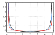
\psfrag{data1}{$\scriptstyle\alpha=1$}\psfrag{data2}{$\scriptstyle\alpha=2$}\psfrag{data3}{$\scriptstyle\alpha=3$}\includegraphics[scale={0.6}]{rate_alpha}

\psfrag{data1}{$\scriptstyle\alpha=1$}\psfrag{data2}{$\scriptstyle\alpha=2$}\psfrag{data3}{$\scriptstyle\alpha=3$}\includegraphics[scale={0.5}]{ddp_alpha}

Figure 9: Large deviations rate function $f(\lambda)$,  its Legendre transform $I(x)$,  and probability density $\propto\exp[-I(x)]$ for different $\alpha\,$ ($N=2$, $\beta_{1}=1$, $\beta_{2}=5$, $r_{2}=r_{1}$, and $V_{1}=V_{2}=0$)

and the large deviation function for energy transfer is,  with $\,\lambda=\lambda_{1}-\lambda_{2}$,

$${}^{\rm th}f(\lambda)=-\int_{0}^{\infty}\ln\frac{{}_{1-{\rm e}^{-2\pi x\beta_{1}}(1-S_{12}^{2}(1-{\rm e}^{-2\pi{\rm i}x\lambda}))-{\rm e}^{-2\pi x\beta_{2}}(1-S_{12}^{2}(1-{\rm e}^{2\pi{\rm i}x\lambda}))+{\rm e}^{-2\pi x(\beta_{1}+\beta_{2})}}}{{}^{(1-{\rm e}^{-2\pi x\beta_{1}})(1-{\rm e}^{-2\pi x\beta_{2}})}}\,{\rm d}x\,,$$ (12.17)

which is illustrated in Fig. 9. The above expression simplifies for $\,\alpha=1\,$ when $\,S_{12}=1$,  reducing again to the relation (12.12) for fully transmitting junction.

12.2 Case $\,M=1$

The case $\,M=1\,$ with the total charge conservation corresponds to the brane $\,{\cal B}\cong U(1)\,$ diagonally embedded into $\,U(1)^{N}$ so that

$$\kappa=(1,\ldots,1)$$ (12.18)

leading to the $S$-matrix

$$S_{ij}=-\rho_{i}\delta_{ij}+\tau_{i}(1-\delta_{ij})$$ (12.19)

where

$$\rho_{i}=\frac{{}_{-r_{i}^{2}+\sum_{k\neq i}r_{k}^{2}}}{{}^{\sum_{k}r_{k}^{2}}},\qquad\tau_{i}=\frac{{}_{2r_{j}^{2}}}{{}^{\sum_{k}r_{k}^{2}}}$$ (12.20)

are the reflection and transmission coefficients. For the equal radii $\,r_{i}=r$,

$$\rho_{i}=\rho=\frac{{}_{N-2}}{{}^{N}},\qquad\tau_{i}=\tau=\frac{{}_{2}}{{}^{N}}$$ (12.21)

leading to a simple nontrivial $S$-matrix

$$S_{ij}=-\rho\delta_{ij}+\tau(1-\delta_{ij})$$ (12.22)

that was already considered in [36], see also [9].

Application to 3 wires

We consider the simplest case with the same radii of compactification. Here we have $\,\rho=1/3\,$ and $\,\tau=2/3\,$ and the $S$-matrix is

$$S=\frac{1}{3}\begin{pmatrix}-1&2&2\\ 2&-1&2\\ 2&2&-1\end{pmatrix}$$ (12.23)

The charge and energy currents are

$$\omega_{neq}(J_{1}^{L})=\frac{{}_{r^{2}\tau}}{{}^{4\pi}}(V_{2}+V_{3}-V_{1})$$ (12.24)

$$\omega_{neq}(K_{1}^{L})=\frac{{}_{r^{2}\tau^{2}}}{{}^{8\pi}}(V_{2}+V_{3}-2V_{1})(V_{1}+V_{2}+V_{3})+\frac{{}_{\pi\tau^{2}}}{{}^{12}}\big{(}\frac{{}_{1}}{{}^{\beta_{2}^{2}}}+\frac{{}_{1}}{{}^{\beta_{3}^{2}}}-\frac{{}_{2}}{{}^{\beta_{1}^{2}}}\big{)}$$ (12.25)

and similarly on the other wires, cyclicly permuting the indices. For the electric and thermal conductance, this gives:

$${}^{{\rm el}}G\,=\,\frac{{}_{r^{2}\tau}}{{}^{4\pi}}\begin{pmatrix}-1&1&1\\ 1&-1&1\\ 1&1&-1\end{pmatrix},\qquad{}^{{\rm th}}G\,=\,\frac{{}_{\pi\tau^{2}}}{{}^{6}}\begin{pmatrix}-2&1&1\\ 1&-2&1\\ 1&1&-2\end{pmatrix}.$$ (12.26)

The large deviation function for the FCS of charge transfers is

$${}^{\rm el}f(\bm{\nu})=\frac{{}_{r^{2}\tau^{2}}}{{}^{8\pi}}\Big{(}\frac{{}_{(2\nu_{1}-\nu_{2}-\nu_{3})^{2}}}{{}^{\beta_{1}}}\ +\ {\rm cycl.}\Big{)}+{\rm i}\frac{{}_{r^{2}\tau}}{{}^{4\pi}}\Big{(}V_{1}(2\nu_{1}-\nu_{2}-\nu_{3})\ +\ {\rm cycl.}\,\Big{)},$$ (12.27)

where “${\rm cycl.}$” stands for terms obtained by cyclic permutation of the indices. The large deviation function for the FCS of energy transfers for $\,V_{i}=0\,$ is:

$${}^{\rm th}f(\bm{\lambda})=-\int_{0}^{\infty}\ln\frac{{}_{N(x,\bm{\lambda})}}{{}^{D(x)}}\,{\rm d}x\qquad$$ (12.28)

where

$$N(x,\bm{\lambda})= \,1-{\rm e}^{-2\pi x(\beta_{1}+\beta_{2}+\beta_{3})}+\rho^{2}\big{(}{\rm e}^{-2\pi x(\beta_{1}+\beta_{2})}\ +\ {\rm cycl.}\,\big{)}-\rho^{2}\big{(}{\rm e}^{-2\pi x\beta_{1}}\ +\ {\rm cycl.}\,\big{)}$$ (12.29)

$$+\tau^{2}\Big{(}{\rm e}^{-2\pi x(\beta_{1}+\beta_{2})}\big{(}{\rm e}^{-2\pi{\rm i}x(\lambda_{2}-\lambda_{3})}+{\rm e}^{-2\pi{\rm i}x(\lambda_{1}-\lambda_{3})}\big{)}\ +\ {\rm cycl.}\,\Big{)}$$ (12.30)

$$-\tau^{2}\Big{(}{\rm e}^{-2\pi x\beta_{1}}\big{(}{\rm e}^{-2\pi{\rm i}x(\lambda_{1}-\lambda_{2})}+{\rm e}^{-2\pi{\rm i}x(\lambda_{1}-\lambda_{3})}\big{)}\ +\ {\rm cycl.}\,\Big{)},$$ (12.31)

$$D(x)= \,(1-{\rm e}^{-2\pi x\beta_{1}})(1-{\rm e}^{-2\pi x\beta_{2}})(1-{\rm e}^{-2\pi x\beta_{3}})\,.$$ (12.32)

Upon the analytic continuation, $\,{}^{\rm th}f(-{\rm i}\bm{\lambda})\equiv f(\lambda_{12},\lambda_{13})\,$ for $\,\lambda_{12}=\lambda_{1}-\lambda_{2}\,$ and $\,\lambda_{13}=\lambda_{1}-\lambda_{3}\,$ which is finite only in the region

$$-\beta_{1}<\lambda_{12}<\beta_{2}\,,\qquad-\beta_{1}<\lambda_{13}<\beta_{3}\,,\qquad-\beta_{2}<\lambda_{13}-\lambda_{12}<\beta_{3}\,.$$ (12.33)

Function $\,f\,$ is plotted in Fig. 10  for $\,(\beta_{1},\beta_{2},\beta_{3})$$=(1,1,1)$ (the equilibrium case) and $\,(\beta_{1},\beta_{2},\beta_{3})=(1,2,3)$ in the coordinate system with axes at $120^{\circ}$ so that the counter-clockwise rotation of the graph by $120^{\circ}$ corresponds to the cyclic permutation $(\lambda_{1},\lambda_{2},\lambda_{3})\mapsto(\lambda_{3},\lambda_{1},\lambda_{2})$.  In equilibrium, $\,f\,$ is symmetric under such a transformation but out of equilibrium, the above $\,\bm{Z}_{3}\,$ symmetry is broken to a degree that may be used as a measure of distance from equilibrium.

\psfrag{title}{$\scriptstyle f(\lambda_{12},\lambda_{12})\ \text{for}\ (\beta_{1},\beta_{2},\beta_{3})=(1,1,1)$ }\psfrag{lambda12}{$\scriptstyle\hskip 8.5359pt\lambda_{12}$}\psfrag{lambda13}{$\scriptstyle\hskip 34.14322pt\lambda_{13}$}\includegraphics[scale={0.655}]{fdev_111}

\psfrag{title}{$\scriptstyle f(\lambda_{12},\lambda_{12})\ \text{for}\ (\beta_{1},\beta_{2},\beta_{3})=(1,1,1)$ }\psfrag{lambda12}{$\scriptstyle\hskip 8.5359pt\lambda_{12}$}\psfrag{lambda13}{$\scriptstyle\hskip 34.14322pt\lambda_{13}$}\psfrag{title}{$\scriptstyle\text{and \,for\ }\ (\beta_{1},\beta_{2},\beta_{3})=(1,2,3)$}\psfrag{lambda13}{$\scriptstyle\hskip 25.6073pt\lambda_{13}$}\psfrag{lambda12}{$\scriptstyle\hskip 8.5359pt\lambda_{12}$}\includegraphics[scale={0.65}]{fdev_123}

Figure 10: Rate function $\,f(\lambda_{12},\lambda_{13})\,$ for  3  wires

The Legendre transform of $\,{}^{\rm th}f(-{\rm i}\bm{\lambda})\,$ is infinite out of the plane $\,x_{1}+x_{2}+x_{3}=0\,$ and on that plane, it may be regarded as a function

$$I(x_{12},x_{13})=\mathop{\rm max}\limits_{\lambda_{12},\lambda_{13}}\,\big{\{}\frac{{}_{1}}{{}^{3}}(2x_{12}\lambda_{12}-x_{12}\lambda_{13}-x_{13}\lambda_{12}+2x_{13}\lambda_{13})-f(\lambda_{12},\lambda_{13})\big{\}}\,.$$ (12.34)

Fig. 11 presents the plot of $\,I(x_{12},x_{13})\,$ for the equilibrium and nonequilibrium choice of temperatures.

\psfrag{title}{$\scriptstyle I(x_{12},x_{12})\ \text{for}\ (\beta_{1},\beta_{2},\beta_{3})=(1,1,1)$ }\psfrag{x12}{$\scriptstyle\hskip 2.84544ptx_{12}$}\psfrag{x13}{$\scriptstyle\hskip 28.45274ptx_{13}$}\includegraphics[scale={0.655}]{rate_111_red}

\psfrag{title}{$\scriptstyle I(x_{12},x_{12})\ \text{for}\ (\beta_{1},\beta_{2},\beta_{3})=(1,1,1)$ }\psfrag{x12}{$\scriptstyle\hskip 2.84544ptx_{12}$}\psfrag{x13}{$\scriptstyle\hskip 28.45274ptx_{13}$}\psfrag{title}{$\scriptstyle\text{and \,for}\ (\beta_{1},\beta_{2},\beta_{3})=(1,2,3)$}\psfrag{x13}{$\scriptstyle\hskip 31.2982ptx_{13}$}\psfrag{x12}{$\scriptstyle\hskip 2.84544ptx_{12}$}\includegraphics[scale={0.65}]{rate_123_red}

Figure 11: Legendre transform $\,I(x_{12},x_{13})\,$ for  3  wires

The level lines of $\,I\,$ are equally spaced in various direction far from the origin, indicating the asymptotic linear increase of the function.  The similar breaking of $\,\bm{Z}_{3}\,$ symmetry as for $\,f\,$ may be observed.

\psfrag{title}{$\scriptstyle\text{normalized}\ \exp[-I(x_{12},x_{12})]\ \text{for}\ (\beta_{1},\beta_{2},\beta_{3})=(1,1,1)$ }\psfrag{x12}{$\scriptstyle\hskip 2.84544ptx_{12}$}\psfrag{x13}{$\scriptstyle\hskip 28.45274ptx_{13}$}\includegraphics[scale={0.655}]{ddp_111}

\psfrag{title}{$\scriptstyle\text{normalized}\ \exp[-I(x_{12},x_{12})]\ \text{for}\ (\beta_{1},\beta_{2},\beta_{3})=(1,1,1)$ }\psfrag{x12}{$\scriptstyle\hskip 2.84544ptx_{12}$}\psfrag{x13}{$\scriptstyle\hskip 28.45274ptx_{13}$}\psfrag{title}{$\scriptstyle\text{and \,for}\ (\beta_{1},\beta_{2},\beta_{3})=(1,2,3)$}\psfrag{x13}{$\scriptstyle\hskip 28.45274ptx_{13}$}\psfrag{x12}{$\scriptstyle\hskip 2.84544ptx_{12}$}\includegraphics[scale={0.65}]{ddp_123}

Figure 12: Probability density $\,\propto\exp[-I(x_{12},x_{13})]\,$ for  3  wires

Finally, Fig. 12 plots for illustration the probability densities $\,\propto\exp[-I(x_{12},x_{13})]$.  Note that most mass of the distribution is in the negative quadrant indicating the heat transfer from the hotter $1^{\rm st}$ and the $2^{\rm nd}$ wires to the colder $3^{\rm rd}$ one.

13 Conclusions

We have studied a model of a junction of $\,N\,$ quantum wires. The Luttinger liquids in the bulk of the wires were represented by a toroidal compactification of the $N$-component massless free bosonic field, with the junction modeled by a simple boundary condition restricting the values of the compactified field to a brane $\,{\cal B}\,$ forming a subgroup isomorphic to $\,U(1)^{M}\,$ of the target torus $\,U(1)^{N}$.  The brane $\,{\cal B}\,$ was assumed to be invariant under the diagonal multiplication by phases in order to assure the global $\,U(1)\,$ invariance and the conservation of the total electric charge. We constructed the theory on the classical and the quantum level and showed that the boundary condition at the junction leads to a linear relation between the right-moving and the left-moving components of the electric currents in different wires. Such a relation describes the scattering by the junction of charges carrying the current. The equilibrium state of the system of connected wires of length $\,L\,$ kept at inverse temperature $\,\beta\,$ and in electric potential $\,V\,$ was discussed in the functional-integral language and in the open-string and closed-string operator formalism, the latter being well suited to describe the thermodynamic limit $\,L\to\infty$.  We obtained the exact solution for the equilibrium current correlation functions both for wires of finite length $\,L\,$ and for $\,L=\infty$.  In the latter case, the resulting theory provides a special case of the system studied in [32] and we adapted from that paper the construction of a stationary nonequilibrium state (NESS) in which the wires are kept at different temperatures and electric potentials. Following the lines of [10, 11], it was shown that such a state is attained at long times if we prepare disjoint semi-infinite wires in equilibrium states at different temperatures and potentials and then connect them by the junction and let the dynamics operate. This is a particular realization of the scenario for construction of quantum nonequilibrium states proposed in [41]. By considering the constructed NESS close to equilibrium, we extracted formulae for the electric and thermal conductance of the junction.

The main result of this paper has been the calculation of the full counting statistics (FCS) for charge and heat transfers through the junction and the analysis of its large deviations asymptotics at long transfer times in the presence of both transmission and reflection of the conserved charges. This was done first for charge, then for heat, and finally, jointly for both. We confirmed by an exact calculation that the large deviations regime of the charge FCS for a junction of semi-infinite wires may be obtained from a large class of limiting procedures sending to infinity the length of the wires as well as the transfer time. The computation of FCS for heat transfers was explicitly done only aligning the length of the wires and the time of the transfer, although we developed tools for performing the general calculation. We expect that the result for the large deviations regime of the FCS for heat transfers obtained in the explicitly treated case applies as well to the situation when the length of the wires is sent to infinity faster than the evolution time. The expressions obtained for the large deviations rate functions of FCS were compared with the ones given by the Levitov-Lesovik formulae. For the charge transfers, we showed that our results for the junctions under consideration differ from the Levitov-Lesovik formula for free fermions, although, for the vanishing Luttinger couplings, some similarity could be observed in the quadratic part of the rate functions that describes the central-limit asymptotics. For the energy transfers through the junction, the part of the FCS that was contributed by the excited bosonic Fock-space modes appeared to coincide with the bosonic Levitov-Lesovik-type formula for FCS obtained in [28].

The simple class of conformal boundary defects considered in the present paper have been chosen for illustrative purpose rather than from phenomenological considerations. The latter might require introducing a larger family of boundary defects. The simplest extension of the class considered here would include conformal boundary defects with displaced branes $\,\bm{g}_{0}{\cal B}\,$ for $\,\bm{g}_{0}\in U(1)^{N}\,$ or/and the ones with added Wilson lines (w.r.t.   a constant gauge field on $\,{\cal B}$). Such boundary defects could be dealt with by the same technique, leading to a richer class of $S$-matrices describing current scattering. More complicated conformal boundary defects would require more powerful boundary CFT techniques for calculation. For the case of vanishing Luttinger couplings, one could use the nonabelian bosonization [48, 6] that comes with a class of conformal boundary defects with nonabelian symmetries. Some partial results in this direction have been already obtained [23]. The other physically relevant question, not disjoint from the previous one, is the stability of the boundary defects in the renormalization group sense. This problem was addressed for some simple cases of junctions in [36, 34, 35]. It can be also studied with the boundary CFT techniques. We postpone a discussion of the above questions to the future research.

Appendix A

Here we shall calculate directly the quantity

$$\omega^{L}_{\beta,V}\Big{(}{\rm e}^{-{\rm i}\nu\int\limits_{0}^{t}J^{\ell}(0,s)\,{\rm d}s}\Big{)}$$ (A.1)

for one wire of length $L>t$ with the Neumann boundary conditions. In this case,

$$J^{\ell}(0,s)\,=\,\frac{{}_{r}}{{}^{4L}}\sum\limits_{n\in\mathbb{Z}}\tilde{\alpha}_{2n}\,{\rm e}^{-\frac{\pi{\rm i}ns}{L}}$$ (A.2)

for $\,\tilde{\alpha}_{2n}=r\alpha_{2n}\,$ and

$$\int\limits_{0}^{t}J^{\ell}(0,s)\,{\rm d}s\,=\,\frac{{}_{ir}}{{}^{4\pi}}\sum\limits_{n\not=0}\frac{{}_{1}}{{}^{n}}\tilde{\alpha}_{2n}\big{(}{\rm e}^{-\frac{\pi{\rm i}nt}{L}}-1\big{)}+\frac{{}_{rt}}{{}^{4L}}\tilde{\alpha}_{0}\,=\,\frac{{}_{r^{2}}}{{}^{4\pi}}\big{(}\varphi^{\ell}(0,t)-\varphi^{\ell}(0,0)\big{)},$$ (A.3)

where the chiral field $\,\varphi^{\ell}\,$ is given by (2.21). We shall reorder the exponential of that operator writing

$${\rm e}^{-{\rm i}\nu\int\limits_{0}^{t}J^{\ell}(0,s)\,{\rm d}s}\,= \,\,{\rm e}^{-{\rm i}\frac{\nu rt}{4L}\tilde{\alpha}_{0}}\,\,{\rm e}^{\frac{{}_{\nu r}}{{}^{4\pi}}\sum\limits_{n<0}\frac{1}{n}\tilde{\alpha}_{2n}\big{(}{\rm e}^{-\frac{\pi{\rm i}nt}{L}}-1\big{)}}\,{\rm e}^{\frac{{}_{\nu r}}{{}^{4\pi}}\sum\limits_{n>0}\frac{1}{n}\tilde{\alpha}_{2n}\big{(}{\rm e}^{-\frac{\pi{\rm i}nt}{L}}-1\big{)}}$$ (A.4)

$$\times\,\,{\rm e}^{-\frac{\nu^{2}r^{2}}{16\pi^{2}}\sum\limits_{n>0}\frac{1}{n}\big{(}2-{\rm e}^{\,\frac{\pi{\rm i}nt}{L}}-{\rm e}^{-\frac{\pi{\rm i}nt}{L}}\big{)}}$$ (A.5)

$$= \,\,{\rm e}^{-{\rm i}\frac{\nu rt}{4L}\tilde{\alpha}_{0}}\,\,{\rm e}^{\frac{{}_{\nu r}}{{}^{4\pi}}\sum\limits_{n<0}\frac{1}{n}\tilde{\alpha}_{2n}\big{(}{\rm e}^{-\frac{\pi{\rm i}nt}{L}}-1\big{)}}\,{\rm e}^{\frac{{}_{\nu r}}{{}^{4\pi}}\sum\limits_{n>0}\frac{1}{n}\tilde{\alpha}_{2n}\big{(}{\rm e}^{-\frac{\pi{\rm i}nt}{L}}-1\big{)}}$$ (A.6)

$$\times\,\,\big{(}4\sin^{2}(\frac{{}_{\pi t}}{{}^{2L}})\big{)}^{-\frac{\nu^{2}r^{2}}{16\pi^{2}}}\,{\rm e}^{-\frac{\nu^{2}r^{2}}{8\pi^{2}}\sum\limits_{n>0}\frac{1}{n}}.$$ (A.7)

Note that the last factor, that may be interpreted as providing the Wick ordering of the left-moving vertex operators $\,{\rm e}^{-{\rm i}\frac{\nu r^{2}}{4\pi}\varphi^{\ell}(0,t)}\,$ and $\,{\rm e}^{\,{\rm i}\frac{\nu r^{2}}{4\pi}\varphi^{\ell}(0,0)}$,  is ultraviolet singular. We shall replace it by its regularized version

$${\rm e}^{-\frac{{}_{\nu^{2}r^{2}}}{{}^{8\pi^{2}}}\sum\limits_{n<\Lambda L}\frac{1}{n}}\equiv\,{\rm e}^{-\frac{{}_{\nu^{2}r^{2}}}{{}^{8\pi^{2}}}C_{\Lambda L}}$$ (A.8)

where $\Lambda$ is the ultraviolet cutoff. This leads to the definition:

$$\Big{(}{\rm e}^{-{\rm i}\nu\int\limits_{0}^{t}J^{\ell}(0,s)\,{\rm d}s}\Big{)}_{{\rm reg}}= \,\,\,{\rm e}^{-{\rm i}\frac{\nu rt}{4L}\tilde{\alpha}_{0}}\,\,{\rm e}^{\frac{{}_{\nu r}}{{}^{4\pi}}\sum\limits_{n<0}\frac{1}{n}\tilde{\alpha}_{2n}\big{(}{\rm e}^{-\frac{\pi{\rm i}nt}{L}}-1\big{)}}\,{\rm e}^{\frac{{}_{\nu r}}{{}^{4\pi}}\sum\limits_{n>0}\frac{1}{n}\tilde{\alpha}_{2n}\big{(}{\rm e}^{-\frac{\pi{\rm i}nt}{L}}-1\big{)}}$$ (A.9)

$$\times\,\,\big{(}4\sin^{2}(\frac{{}_{\pi t}}{{}^{2L}})\big{)}^{-\frac{\nu^{2}r^{2}}{16\pi^{2}}}\,\,{\rm e}^{-\frac{{}_{\nu^{2}r^{2}}}{{}^{8\pi^{2}}}\sum\limits_{n<\Lambda L}\frac{1}{n}}\,.$$ (A.10)

The commutation relation

$$\Big{[}{\rm e}^{\pm\frac{{}_{\nu r}}{{}^{4\pi}}\sum\limits_{n>0}\frac{1}{n}\tilde{\alpha}_{2n}\big{(}{\rm e}^{-\frac{\pi{\rm i}nt}{L}}-1\big{)}},\tilde{\alpha}_{-2m}\Big{]}\,=\,\pm\frac{{}_{\nu r}}{{}^{2\pi}}\big{(}{\rm e}^{-\frac{\pi{\rm i}mt}{L}}-1\big{)}\,{\rm e}^{\pm\frac{{}_{\nu r}}{{}^{4\pi}}\sum\limits_{n>0}\frac{1}{n}\tilde{\alpha}_{2n}\big{(}{\rm e}^{-\frac{\pi{\rm i}nt}{L}}-1\big{)}},$$ (A.11)

implies that

$${\rm e}^{\pm\frac{{}_{\nu r}}{{}^{4\pi}}\sum\limits_{n>0}\frac{1}{n}\tilde{\alpha}_{2n}\big{(}{\rm e}^{-\frac{\pi{\rm i}nt}{L}}-1\big{)}}(\tilde{\alpha}_{-2m})^{p}|0\rangle\,=\,\sum\limits_{k=0}^{p}(\pm 1)^{k}\big{(}\begin{subarray}{c}{{p}}\\ {k}\end{subarray}\big{)}\big{(}\frac{{}_{\nu r}}{{}^{2\pi}}\big{(}{\rm e}^{-\frac{\pi{\rm i}mt}{L}}-1\big{)}\big{)}^{k}\,(\tilde{\alpha}_{-2m})^{p-k}|0\rangle\,.$$ (A.12)

Hence

$$\frac{\big{\langle}0\big{|}\,(\tilde{\alpha}_{2m})^{p}\,{\rm e}^{\frac{{}_{\nu r}}{{}^{4\pi}}\sum\limits_{n<0}\frac{1}{n}\tilde{\alpha}_{2n}\big{(}{\rm e}^{-\frac{\pi{\rm i}nt}{L}}-1\big{)}}\,{\rm e}^{\frac{{}_{\nu r}}{{}^{4\pi}}\sum\limits_{n>0}\frac{1}{n}\tilde{\alpha}_{2n}\big{(}{\rm e}^{-\frac{\pi{\rm i}nt}{L}}-1\big{)}}(\tilde{\alpha}_{-2m})^{p}\big{|}0\big{\rangle}}{p!(2m)^{p}}$$ (A.13)

$$=\,\frac{{}_{1}}{{}^{p!(2m)^{p}}}\,\sum\limits_{k=0}^{p}(-1)^{k}\big{(}\begin{subarray}{c}{p}\\ {k}\end{subarray}\big{)}^{2}\big{(}\frac{{}_{\nu^{2}r^{2}}}{{}^{4\pi^{2}}}\big{|}{\rm e}^{-\frac{\pi{\rm i}mt}{L}}-1\big{|}^{2}\big{)}^{k}(p-k)!(2m)^{p-k}$$ (A.14)

$$=\,\sum\limits_{k=0}^{p}(-1)^{k}\big{(}\begin{subarray}{c}{p}\\ {k}\end{subarray}\big{)}\frac{{}_{1}}{{}^{k!(2m)^{k}}}\big{(}\frac{{}_{\nu^{2}r^{2}}}{{}^{\pi^{2}}}\sin^{2}({\frac{{}_{\pi mt}}{{}^{2L}}})\big{)}^{k}.$$ (A.15)

The orthonormal basis of the Fock space ${\mathcal{F}}_{e}$ is given by the vectors

$$\prod\limits_{m=1}^{\infty}\frac{{}_{(\tilde{\alpha}_{-2m})^{p_{m}}}}{{}^{\sqrt{p_{m}!(2m)^{p_{m}}}}}\,\big{|}0\big{\rangle}$$ (A.16)

with all but a finite number of $\,p_{m}=0,1,\dots\,$ equal to zero. Such vectors are eigenvectors of the Hamiltonian $\,H^{0}\,$ with eigenvalues $\,\frac{\pi}{2L}\big{(}\sum\limits_{m=1}^{\infty}2mp_{m}\,-\frac{1}{8}\big{)}\,$ and are annihilated by $\,Q^{0}$.  Hence

$${\rm tr}_{{\mathcal{F}}_{e}}\,{\rm e}^{-\beta(H^{0}-VQ^{0})}\,{\rm e}^{\frac{{}_{\nu r}}{{}^{4\pi}}\sum\limits_{n<0}\frac{1}{n}\tilde{\alpha}_{2n}\big{(}{\rm e}^{-\frac{\pi{\rm i}nt}{L}}-1\big{)}}\,{\rm e}^{\frac{{}_{\nu r}}{{}^{4\pi}}\sum\limits_{n>0}\frac{1}{n}\tilde{\alpha}_{2n}\big{(}{\rm e}^{-\frac{\pi{\rm i}nt}{L}}-1\big{)}}$$ (A.17)

$$=\,{\rm e}^{\frac{\pi\beta}{16L}}\prod\limits_{m=1}^{\infty}\Big{(}\sum\limits_{p=1}^{\infty}{\rm e}^{-\frac{\pi\beta}{L}pm}\sum\limits_{k=0}^{p}(-1)^{k}\big{(}\begin{subarray}{c}{p}\\ {k}\end{subarray}\big{)}\frac{{}_{1}}{{}^{k!(2m)^{k}}}\big{(}\frac{{}_{\nu^{2}r^{2}}}{{}^{\pi^{2}}}\sin^{2}({\frac{{}_{\pi mt}}{{}^{2L}}})\big{)}^{k}\Big{)}$$ (A.18)

$$=\,{\rm e}^{\frac{\pi\beta}{16L}}\prod\limits_{m=1}^{\infty}\Big{(}\sum\limits_{k=0}^{\infty}\frac{{}_{(-1)^{k}}}{{}^{(k!)^{2}(2m)^{k}}}\big{(}\frac{{}_{\nu^{2}r^{2}}}{{}^{\pi^{2}}}\sin^{2}(\frac{{}_{\pi mt}}{{}^{2L}})\big{)}^{k}\sum\limits_{p=k}^{\infty}p(p-1)\cdots(p-k+1)\,{\rm e}^{-\frac{\pi\beta}{L}pm}\Big{)}.\qquad$$ (A.19)

Since by a straightforward calculation

$$\sum\limits_{p=k}^{\infty}p(p-1)\cdots(p-k+1)z^{p}\,=\,\frac{{}_{k!z^{k}}}{{}^{(1-z)^{k+1}}}$$ (A.20)

for $\,|z|<1$,  we infer that

$${\rm tr}_{{\mathcal{F}}_{e}}\,{\rm e}^{-\beta(H^{0}-VQ^{0})}\,{\rm e}^{\frac{{}_{\nu r}}{{}^{4\pi}}\sum\limits_{n<0}\frac{1}{n}\tilde{\alpha}_{2n}\big{(}{\rm e}^{-\frac{\pi{\rm i}nt}{L}}-1\big{)}}\,{\rm e}^{\frac{{}_{\nu r}}{{}^{4\pi}}\sum\limits_{n>0}\frac{1}{n}\tilde{\alpha}_{2n}\big{(}{\rm e}^{-\frac{\pi{\rm i}nt}{L}}-1\big{)}}$$ (A.21)

$$=\,{\rm e}^{\frac{\pi\beta}{16L}}\prod\limits_{m=1}^{\infty}\Big{(}\sum\limits_{k=0}^{\infty}\frac{{}_{(-1)^{k}}}{{}^{k!(2m)^{k}}}\big{(}\frac{{}_{\nu^{2}r^{2}}}{{}^{\pi^{2}}}\sin^{2}(\frac{{}_{\pi mt}}{{}^{2L}})\big{)}^{k}\frac{{}_{{\rm e}^{-\frac{\pi\beta}{L}mk}}}{{}^{(1-{\rm e}^{-\frac{\pi\beta}{L}m})^{k+1}}}\Big{)}$$ (A.22)

$$=\,{\rm e}^{\frac{\pi\beta}{16L}}\prod\limits_{m=1}^{\infty}\Big{(}\exp\Big{[}-\frac{{}_{\nu^{2}r^{2}}}{{}^{2\pi^{2}m}}\sin^{2}(\frac{{}_{\pi mt}}{{}^{2L}})\,\frac{{}_{{\rm e}^{-\frac{\pi\beta}{L}m}}}{{}^{1-{\rm e}^{-\frac{\pi\beta}{L}m}}}\Big{]}\Big{)}\prod\limits_{m=1}^{\infty}\frac{{}_{1}}{{}^{1-{\rm e}^{-\frac{\pi\beta}{L}m}}}\,.$$ (A.23)

The trace over the zero mode space $\,{\cal H}_{0}\,$ spanned by the orthonormal vectors $\,|k\rangle\,$ with $\,k\in\mathbb{Z}\,$ such that $\,\tilde{\alpha}_{0}|k\rangle=2r^{-1}|k\rangle\,$ is

$${\rm tr}_{{\cal H}_{0}}\,{\rm e}^{-\beta(H^{0}-VQ^{0})}\,{\rm e}^{-{\rm i}\nu\frac{rt}{4L}\tilde{\alpha}_{0}}=\sum\limits_{q\in\mathbb{Z}}{\rm e}^{-\frac{\pi\beta}{Lr^{2}}k^{2}+\beta Vk-{\rm i}\nu\frac{t}{2L}k}\,.$$ (A.24)

Multiplying those two traces and the factor of the last line of (A.10) and dividing them by the partition function, we obtain the expression

$$\omega^{L}_{\beta,V}\Big{(}\Big{(}{\rm e}^{-{\rm i}\nu\int\limits_{0}^{t}J^{\ell}(0,s)\,{\rm d}s}\Big{)}_{\rm reg}\Big{)}\,= \,\,\big{(}4\sin^{2}(\frac{{}_{\pi t}}{{}^{2L}})\big{)}^{-\frac{\nu^{2}r^{2}}{16\pi^{2}}}\ {\rm e}^{-\frac{{}_{\nu^{2}r^{2}}}{{}^{8\pi^{2}}}\sum\limits_{n<\Lambda L}\frac{1}{n}}\ \frac{{}_{\sum\limits_{k\in\mathbb{Z}}{\rm e}^{-\frac{\pi\beta}{Lr^{2}}k^{2}+\beta Vk-{\rm i}\nu\frac{t}{2L}k}}}{{}^{\sum\limits_{k\in\mathbb{Z}}{\rm e}^{-\frac{\pi\beta}{Lr^{2}}k^{2}+\beta Vk}}}$$ (A.25)

$$\times\,\,\prod\limits_{m=1}^{\infty}\Big{(}\exp\Big{[}-\frac{{}_{\nu^{2}r^{2}}}{{}^{2\pi^{2}m}}\sin^{2}(\frac{{}_{\pi mt}}{{}^{2L}})\,\frac{{}_{{\rm e}^{-\frac{\pi\beta}{L}m}}}{{}^{1-{\rm e}^{-\frac{\pi\beta}{L}m}}}\Big{]}\Big{)}.$$ (A.26)

By Eq. 16.30.1 of [5],

$$4\sum\limits_{m=1}^{\infty}\frac{{}_{1}}{{}^{m}}\sin^{2}(\frac{{}_{\pi mt}}{{}^{2L}})\,\frac{{}_{{\rm e}^{-\frac{\pi\beta}{L}m}}}{{}^{1-{\rm e}^{-\frac{\pi\beta}{L}m}}}=\ln\frac{{}_{\pi\,\theta_{1}(\frac{{\rm i}\beta}{2L};\frac{t}{2L})}}{{}^{\sin(\frac{\pi t}{2L})\,\partial_{z}\theta_{1}(\frac{{\rm i}\beta}{2L};0)}}\,,$$ (A.27)

where we use the definition

$$\theta_{1}(\tau;z)=\sum\limits_{n\in\mathbb{Z}}{\rm e}^{\pi{\rm i}\tau(n+\frac{1}{2})^{2}+2\pi i(n+\frac{1}{2})(z+\frac{1}{2})}$$ (A.28)

for the first of the Jacobi theta-functions. Hence (A.26) may be rewritten in the form

$$\omega^{L}_{\beta,V}\Big{(}\Big{(}{\rm e}^{-{\rm i}\nu\int\limits_{0}^{t}J^{\ell}(0,s)\,{\rm d}s}\Big{)}_{\rm reg}\Big{)}\,= \,\,\exp\Big{[}-\frac{{}_{\nu^{2}r^{2}}}{{}^{8\pi^{2}}}\big{(}\sum\limits_{n<\Lambda L}\frac{{}_{1}}{{}^{n}}\,+\,\ln\frac{{}_{2\pi\,\theta_{1}(\frac{{\rm i}\beta}{2L};\frac{t}{2L})}}{{}^{\partial_{z}\theta_{1}(\frac{i\beta}{2L};0)}}\Big{)}\Big{]}$$ (A.29)

$$\times\,\,\frac{{}_{\sum\limits_{k\in\mathbb{Z}}{\rm e}^{-\frac{\pi\beta}{Lr^{2}}k^{2}+\beta Vk-{\rm i}\nu\frac{t}{2L}k}}}{{}^{\sum\limits_{k\in\mathbb{Z}}{\rm e}^{-\frac{\pi\beta}{Lr^{2}}k^{2}+\beta Vk}}}$$ (A.30)

The substitution of the above relation to the (ultraviolet regularized version of) (10.14) results in the identity (10.34).

Appendix B

Let us consider a quadratic selfadjoint operator

$${\cal A}\,=\,\sum\limits_{i,i^{\prime}=1}^{N}\sum\limits_{n,n^{\prime}=1}^{\infty}\big{(}\frac{{}_{1}}{{}^{2}}A_{ni,n^{\prime}i^{\prime}}\,a^{\dagger}_{ni}a^{\dagger}_{n^{\prime}i^{\prime}}+B_{ni,n^{\prime}i^{\prime}}\,a^{\dagger}_{ni}a_{n^{\prime}i^{\prime}}+\frac{{}_{1}}{{}^{2}}\overline{A_{ni,n^{\prime}i^{\prime}}}\,a_{ni}a_{n^{\prime}i^{\prime}}\big{)}$$ (B.1)

acting in the Fock space ${\mathcal{F}}$ of the vacuum representation of the canonical commutation relations (CCR)

$$[a_{ni},a_{n^{\prime}i^{\prime}}]=0=[a^{\dagger}_{ni},a^{\dagger}_{n^{\prime}i^{\prime}}]\,,\qquad[a_{ni},a^{\dagger}_{n^{\prime}i^{\prime}}]=\delta_{ii^{\prime}}\delta_{n,-n^{\prime}}$$ (B.2)

built on the normalized vacuum state $|0\rangle$ annihilated by operators $a_{ni}$. We assume that $A_{ni,n^{\prime}i^{\prime}}=A_{n^{\prime}i^{\prime},ni}$ and $B_{ni,n^{\prime}i^{\prime}}=\overline{B_{n^{\prime}i^{\prime},ni}}$.  Note the commutation relations

$$\bigg{[}{\cal A}\,,\bigg{(}\begin{matrix}a^{\dagger}_{ni}\cr a_{ni}\end{matrix}\bigg{)}\bigg{]}=\sum_{i^{\prime}}\sum_{n^{\prime}>0}\bigg{(}\begin{matrix}\overline{B_{in,i^{\prime}n^{\prime}}}&\overline{A_{in,i^{\prime}n^{\prime}}}\cr-A_{in,i^{\prime}n^{\prime}}&-B_{in,i^{\prime}n^{\prime}}\end{matrix}\bigg{)}\bigg{(}\begin{matrix}a^{\dagger}_{n^{\prime}i^{\prime}}\cr a_{n^{\prime}i^{\prime}}\end{matrix}\bigg{)}.$$ (B.3)

The exponentiation of the above relation gives

$${\rm e}^{\hskip 0.85355pt{\rm i}{\cal A}}\bigg{(}\begin{matrix}a^{\dagger}_{ni}\cr a_{ni}\end{matrix}\bigg{)}{\rm e}^{-{\rm i}{\cal A}}=\sum_{i^{\prime}}\sum_{n^{\prime}>0}\bigg{(}\begin{matrix}\overline{P_{in,i^{\prime}n^{\prime}}}&\overline{Q_{in,i^{\prime}n^{\prime}}}\cr Q_{in,i^{\prime}n^{\prime}}&P_{in,i^{\prime}n^{\prime}}\end{matrix}\bigg{)}\bigg{(}\begin{matrix}a^{\dagger}_{n^{\prime}i^{\prime}}\cr a_{n^{\prime}i^{\prime}}\end{matrix}\bigg{)},$$ (B.4)

where, in the language of infinite matrices,

$$\bigg{(}\begin{matrix}\overline{P}&\overline{Q}\cr Q&P\end{matrix}\bigg{)}\,=\,\exp\bigg{(}\begin{matrix}\overline{B}&\overline{A}\cr-A&-B\end{matrix}\bigg{)}.$$ (B.5)

One of the results of the theory of the Bogoliubov transformations associated to the quadratic Hamiltonians $\,{\cal A}\,$ is the formula

$$\big{\langle}0\big{|}{\rm e}^{i{\cal A}}\big{|}0\rangle\,=\,\det\big{(}{\rm e}^{iB}P\big{)}^{-1/2}$$ (B.6)

holding under conditions that guarantee the finiteness of the left and right hand sides which will be satisfied in the cases of interest for us,  see e.g. [17].

We shall need a generalization of that formula to the expectations of operator $\,{\rm e}^{i{\cal A}}\,$ in certain mixed states. Consider such a state $\,\omega_{\rho}$ corresponding to the density matrix

$$\rho\,=\,\frac{{}_{1}}{{}^{Z}}\,{\rm e}^{-\sum\limits_{i=1}^{N}\sum\limits_{n=1}^{\infty}\epsilon_{ni}\,a^{\dagger}_{ni}a_{ni}}\,,$$ (B.7)

with $\,\epsilon_{in}>0\,$ diverging sufficiently fast when $\,n\to\infty\,$ and the normalization factor

$$Z\,=\,\prod\limits_{i=1}^{N}\prod\limits_{n=1}^{\infty}(1-{\rm e}^{-\epsilon_{ni}})^{-1}.$$ (B.8)

We would like to calculate the expectation value $\,\omega_{\rho}\big{(}{\rm e}^{i{\cal A}}\big{)}$.  To this end, we may use the Araki-Woods representation [3] of the CCR acting in the double Fock space $\,{\mathcal{F}}\otimes{\mathcal{F}}\,$ and given by the formula

$$\bigg{(}\begin{matrix}a_{ni}^{\dagger}\cr a_{ni}\end{matrix}\bigg{)}\,\longmapsto\,\bigg{(}\begin{matrix}\hat{a}_{ni}^{\dagger}\cr\hat{a}_{ni}\end{matrix}\bigg{)}=\bigg{(}\begin{matrix}\sqrt{1+b_{ni}}\,(a^{1}_{ni})^{\dagger}+\sqrt{b_{ni}}\,a^{2}_{ni}\cr\sqrt{1+b_{ni}}\,a^{1}_{ni}+\sqrt{b_{ni}}\,(a^{2}_{ni})^{\dagger}\end{matrix}\bigg{)},$$ (B.9)

where

$$b_{ni}=\frac{1}{{\rm e}^{\epsilon_{ni}}-1}\,,\qquad a^{1}_{ni}=a_{ni}\otimes I\,,\qquad a^{2}_{ni}=I\otimes a_{ni}\,.$$ (B.10)

The Araki-Woods representation has the property that the matrix element on the vacuum $|0,0\rangle=|0\rangle\otimes|0\rangle$ of a CCR observables taken in that representation reproduces their $\omega_{\rho}$ expectations. In particular

$$\omega_{\rho}\big{(}{\rm e}^{\hskip 0.85355pt{\rm i}{\cal A}}\big{)}\,=\,{\rm tr}_{{}_{\mathcal{F}}}\Big{(}\rho\,{\rm e}^{\hskip 0.85355pt{\rm i}{\cal A}}\Big{)}\,=\,\big{\langle}0,0\big{|}{\rm e}^{i\hat{\cal A}}\big{|}0,0\big{\rangle}\,,$$ (B.11)

where

$$\hat{\cal A}\,=\,\sum\limits_{i=1}^{N}\sum\limits_{n=1}^{\infty}\big{(}\frac{{}_{1}}{{}^{2}}A_{ni,n^{\prime}i^{\prime}}\,\hat{a}^{\dagger}_{ni}\hat{a}^{\dagger}_{n^{\prime}i^{\prime}}+B_{ni,n^{\prime}i^{\prime}}\hat{a}^{\dagger}_{ni}\,\hat{a}_{ni}+\frac{{}_{1}}{{}^{2}}\overline{A_{ni,n^{\prime}i^{\prime}}}\,\hat{a}_{ni}\hat{a}_{n^{\prime}i^{\prime}}\big{)}$$ (B.12)

$$=\,\sum\limits_{\sigma,\sigma^{\prime}=1}^{2}\sum\limits_{i=1}^{N}\sum\limits_{n=1}^{\infty}\big{(}\frac{{}_{1}}{{}^{2}}\hat{A}^{\sigma,\sigma^{\prime}}_{ni,n^{\prime}i^{\prime}}(\hat{a}^{\sigma}_{ni})^{\dagger}({\hat{a}}^{\sigma^{\prime}}_{n^{\prime}i^{\prime}})^{\dagger}+\hat{B}^{\sigma,\sigma^{\prime}}_{ni,n^{\prime}i^{\prime}}({\hat{a}}^{\sigma}_{ni})^{\dagger}{\hat{a}}^{\sigma^{\prime}}_{n^{\prime}i^{\prime}}+\frac{{}_{1}}{{}^{2}}\overline{\hat{A}^{\sigma,\sigma^{\prime}}_{ni,n^{\prime}i^{\prime}}}{\hat{a}}^{\sigma}_{ni}{\hat{a}}^{\sigma^{\prime}}_{n^{\prime}i^{\prime}}\big{)}$$ (B.13)

$$\hskip 8.5359pt+\sum\limits_{i=1}^{N}\sum\limits_{n=1}^{N}B_{ni,ni}b_{ni}\,,$$ (B.14)

with

$$\bigg{(}\begin{matrix}\hat{A}^{1,1}_{ni,n^{\prime}i^{\prime}}&\hat{A}^{1,2}_{ni,n^{\prime}i^{\prime}}\cr\hat{A}^{2,1}_{ni,n^{\prime}i^{\prime}}&\hat{A}^{2,2}_{ni,n^{\prime}i^{\prime}}\end{matrix}\bigg{)}\,=\,\bigg{(}\begin{matrix}A_{ni,n^{\prime}i^{\prime}}\sqrt{(1+b_{ni})(1+b_{n^{\prime}i^{\prime}})}&B_{ni,n^{\prime}i^{\prime}}\sqrt{(1+b_{ni})b_{n^{\prime}i^{\prime}}}\cr\overline{B_{ni,n^{\prime}i^{\prime}}}\sqrt{b_{ni}(1+b_{n^{\prime}i^{\prime}})}&\overline{A_{ni,n^{\prime}i^{\prime}}}\sqrt{b_{ni}b_{n^{\prime}i^{\prime}}}\end{matrix}\bigg{)},$$ (B.15)

$$\bigg{(}\begin{matrix}\hat{B}^{1,1}_{ni,n^{\prime}i^{\prime}}&\hat{B}^{1,2}_{ni,n^{\prime}i^{\prime}}\cr\hat{B}^{2,1}_{ni,n^{\prime}i^{\prime}}&\hat{B}^{2,2}_{ni,n^{\prime}i^{\prime}}\end{matrix}\bigg{)}\,=\,\bigg{(}\begin{matrix}B_{ni,n^{\prime}i^{\prime}}\sqrt{(1+b_{ni})(1+b_{n^{\prime}i^{\prime}})}&A_{ni,n^{\prime}1^{\prime}}\sqrt{(1+b_{ni})b_{n^{\prime}i^{\prime}}}\cr\overline{A_{ni,n^{\prime}1^{\prime}}}\sqrt{b_{ni}(1+b_{n^{\prime}i^{\prime}})}&\overline{B_{ni,n^{\prime}i^{\prime}}}\sqrt{b_{ni}b_{n^{\prime}i^{\prime}}}\end{matrix}\bigg{)}.$$ (B.16)

Denoting

$$\exp\bigg{[}{\rm i}\bigg{(}\begin{matrix}\overline{\hat{B}}&\overline{\hat{A}}\cr-\hat{A}&-\hat{B}\end{matrix}\bigg{)}\bigg{]}\,\equiv\,\bigg{(}\begin{matrix}\overline{\hat{P}}&\overline{\hat{Q}}\cr\hat{Q}&\hat{P}\end{matrix}\bigg{)},$$ (B.17)

we infer from the previous result (B.6) that

$$\omega_{\rho}\big{(}{\rm e}^{\hskip 0.85355pt{\rm i}{\cal A}}\big{)}\,=\,{\rm e}^{i\sum\limits_{i,n}B_{in,in}b_{ni}}\det\big{(}{\rm e}^{{\rm i}\hat{B}}\hat{P}\big{)}^{-1/2}\,.$$ (B.18)

The above calculation can be applied to the operator ${\cal A}$ corresponding to the excited modes part of $\,\sum\limits_{i}\lambda_{i}\big{(}H_{i}^{0}+\Delta H_{i}(t)\big{)}\,$ for any time $\,t$,  but we shall limit ourselves to the simpler instance when $\,t=2L$.  In that case

$${\cal A}\,=\,\frac{{}_{\pi}}{{}^{L}}\sum\limits_{i,i^{\prime}}(O\lambda O)_{ii^{\prime}}\sum\limits_{n=1}^{\infty}\tilde{\alpha}_{(-2n)i}\tilde{\alpha}_{(2n)i^{\prime}}\,,$$ (B.19)

see (10.58),  with the identification

$$\frac{{}_{\tilde{\alpha}_{(2n)i}}}{{}^{(2n)^{1/2}}}\equiv a_{ni}\,,\qquad\frac{{}_{\tilde{\alpha}_{(-2n)i}}}{{}^{(2n)^{1/2}}}\equiv a^{\dagger}_{ni}\,,$$ (B.20)

so that

$$A_{ni,n^{\prime}i^{\prime}}=0\,,\qquad B_{ni,n^{\prime}i^{\prime}}=\frac{{}_{2\pi}}{{}^{L}}(O\lambda O)_{ii^{\prime}}n\,\delta_{nn^{\prime}}\,.$$ (B.21)

For the density matrix, we shall take

$$\rho\,=\,\frac{{}_{1}}{{}^{Z_{\beta}}}\,{\rm e}^{-\frac{\pi}{2L}\sum\limits_{i}\beta_{i}\sum\limits_{n>0}\tilde{\alpha}_{(-2n)i}\tilde{\alpha}_{(2n)i}}$$ (B.22)

so that the state $\,\omega_{\rho}\,$ coincides with $\,\omega_{0}^{L}\,$ on the algebra generated by the excited modes. The normalization

$$Z_{\beta}\,=\,\prod\limits_{i,n>0}(1-{\rm e}^{-\frac{\pi n\beta_{i}}{L}})^{-1}\,.$$ (B.23)

In this case $b_{ni}=({\rm e}^{\frac{\pi}{L}n\beta_{i}}-1)^{-1}$.  It follows that

$$\bigg{(}\begin{matrix}\hat{A}^{1,1}_{ni,n^{\prime}i^{\prime}}&\hat{A}^{1,2}_{ni,n^{\prime}i^{\prime}}\cr\hat{A}^{2,1}_{ni,n^{\prime}i^{\prime}}&\hat{A}^{2,2}_{ni,n^{\prime}i^{\prime}}\end{matrix}\bigg{)}=\frac{{}_{\pi}}{{}^{L}}n\,\delta_{nn^{\prime}}\bigg{(}\begin{matrix}0&(O\lambda O)_{ii^{\prime}}\sqrt{(1+b_{ni})b_{ni^{\prime}}}\cr(O\lambda O)_{ii^{\prime}}\sqrt{b_{ni}(1+b_{ni^{\prime}})}&0\end{matrix}\bigg{)},$$ (B.24)

$$\bigg{(}\begin{matrix}\hat{B}^{1,1}_{ni,n^{\prime}i^{\prime}}&\hat{B}^{1,2}_{ni,n^{\prime}i^{\prime}}\cr\hat{B}^{2,1}_{ni,n^{\prime}i^{\prime}}&\hat{B}^{2,2}_{ni,n^{\prime}i^{\prime}}\end{matrix}\bigg{)}=\frac{{}_{\pi}}{{}^{L}}n\,\delta_{nn^{\prime}}\bigg{(}\begin{matrix}(O\lambda O)_{ii^{\prime}}\sqrt{(1+b_{ni})(1+b_{ni^{\prime}})}&0\cr 0&(O\lambda O)_{ii^{\prime}}\sqrt{b_{ni}b_{ni^{\prime}}}\end{matrix}\bigg{)}.$$ (B.25)

A little of straightforward algebra shows that

$$\bigg{(}\begin{matrix}\hat{P}^{1,1}_{ni,n^{\prime}i^{\prime}}&\hat{P}^{1,2}_{ni,n^{\prime}i^{\prime}}\cr\hat{P}^{2,1}_{ni,n^{\prime}i^{\prime}}&\hat{P}^{2,2}_{ni,n^{\prime}i^{\prime}}\end{matrix}\bigg{)}=\delta_{nn^{\prime}}\delta_{ii^{\prime}}\bigg{(}\begin{matrix}1&0\cr 0&1\end{matrix}\bigg{)}$$ (B.26)

$$+\delta_{nn^{\prime}}\bigg{(}\begin{matrix}\big{(}O\,{\rm e}^{-\frac{\pi{\rm i}}{L}n\lambda}O-I\big{)}_{ii^{\prime}}\sqrt{(1+b_{ni})(1+b_{ni^{\prime}})}&0\cr 0&-\big{(}O\,{\rm e}^{\frac{\pi{\rm i}}{L}n\lambda}O-I\big{)}_{ii^{\prime}}\sqrt{b_{ni}b_{ni^{\prime}}}\end{matrix}\bigg{)},\quad$$ (B.27)

$$\bigg{(}\begin{matrix}\hat{Q}^{1,1}_{ni,n^{\prime}i^{\prime}}&\hat{Q}^{1,2}_{ni,n^{\prime}i^{\prime}}\cr\hat{Q}^{2,1}_{ni,n^{\prime}i^{\prime}}&\hat{Q}^{2,2}_{ni,n^{\prime}i^{\prime}}\end{matrix}\bigg{)}$$ (B.28)

$$=\delta_{nn^{\prime}}\bigg{(}\begin{matrix}0&\big{(}O\,{\rm e}^{-\frac{\pi{\rm i}}{L}n\lambda}O-I\big{)}_{ii^{\prime}}\sqrt{(1+b_{ni})b_{ni^{\prime}}}\cr-\big{(}O\,{\rm e}^{\frac{\pi{\rm i}}{L}n\lambda}O-I\big{)}_{ii^{\prime}}\sqrt{b_{ni}(1+b_{ni^{\prime}})}&0\end{matrix}\bigg{)},\quad$$ (B.29)

Hence, denoting by $b_{n}$ the diagonal $N\times N$ matrix with entries $b_{ni}$, we obtain

$$\det\big{(}\hat{P}_{n,n}\big{)}^{-{1/2}}\, =\,\bigg{(}\det\Big{(}I+\big{(}O\,{\rm e}^{-\frac{\pi{\rm i}}{L}n\lambda}O-I\big{)}(I+b_{n})\Big{)}\det\Big{(}I-\big{(}O\,{\rm e}^{\frac{\pi{\rm i}}{L}n\lambda}O-I\big{)}b_{n}\Big{)}\bigg{)}^{-1/2}$$ (B.30)

$$=\,\bigg{(}\det\Big{(}O\,{\rm e}^{-\frac{\pi{\rm i}}{L}n\lambda}O\Big{)}\det\Big{(}I+\big{(}I-O\,{\rm e}^{\frac{\pi{\rm i}}{L}n\lambda}O\big{)}b_{n}\Big{)}^{2}\bigg{)}^{-1/2}$$ (B.31)

$$=\,{\rm e}^{\frac{\pi{\rm i}}{2L}n\sum\limits_{i}\lambda_{i}}\,\det\Big{(}I+\big{(}I-O\,{\rm e}^{\frac{\pi{\rm i}}{L}n\lambda}O\big{)}b_{n}\Big{)}^{-1}.$$ (B.32)

On the other hand,

$${\rm e}^{{\rm i}\sum\limits_{i}B_{ni,ni}b_{ni}}\,\det\big{(}{\rm e}^{i\hat{B}_{n,n}}\big{)}^{-1/2}={\rm e}^{\frac{\pi{\rm i}}{L}n\sum\limits_{i}(O\lambda O)_{ii}b_{ni}-\frac{\pi{\rm i}}{2L}n\sum\limits_{i}(O\lambda O)_{ii}(1+2b_{ni})}={\rm e}^{-\frac{\pi{\rm i}}{2L}n\sum\limits_{i}\lambda_{i}}.$$ (B.33)

We infer then from (B.18) that

$${\rm tr}_{{}_{\mathcal{F}}}\Big{(}\rho\,{\rm e}^{i{\cal A}}\Big{)}\,=\,\prod\limits_{n=1}^{\infty}\det\Big{(}I+\big{(}I-O\,{\rm e}^{\frac{\pi{\rm i}}{L}n\lambda}O\big{)}\big{(}{\rm e}^{\frac{\pi}{L}n\beta}-I\big{)}^{-1}\Big{)}^{-1}.$$ (B.34)

What we have to compute, however, is the contribution of the excited modes to (10.59) which is equal to

$$\frac{{}_{1}}{{}^{Z_{\beta}}}\,{\rm tr}\Big{(}{\rm e}^{-\frac{\pi}{2L}\sum\limits_{i}(\beta_{i}+{\rm i}\lambda_{i})\sum\limits_{n>0}\alpha_{(-2n)i}\tilde{\alpha}_{(2n)i}}\,{\rm e}^{i{\cal A}}\Big{)}.$$ (B.35)

This is clearly obtained by multiplying (B.34) by $\,Z_{\beta}$,  shifting $\,\beta\,$ to $\,\beta+i\lambda\,$ in the result, and re-dividing it by $\,Z_{\beta}$,  which gives

$$\prod\limits_{n=1}^{\infty}\bigg{(}\frac{{}_{\det\big{(}I-{\rm e}^{-\frac{\pi}{L}n\beta}\big{)}}}{{}^{\det\big{(}I-{\rm e}^{-\frac{\pi}{L}n(\beta+i\lambda)}\big{)}}}\det\Big{(}I+\big{(}I-O\,{\rm e}^{\frac{\pi{\rm i}}{L}n\lambda}O\big{)}\big{(}{\rm e}^{\frac{\pi}{L}n(\beta+i\lambda)}-I\big{)}^{-1}\Big{)}^{-1}\bigg{)}$$ (B.36)

$$=\,\prod\limits_{n=1}^{\infty}\det\Big{(}I+\big{(}I-{\rm e}^{-\frac{\pi{\rm i}}{L}n\lambda}O\,{\rm e}^{\frac{\pi{\rm i}}{L}n\lambda}O\big{)}({\rm e}^{\frac{\pi}{L}n\beta}-I)^{-1}\Big{)}^{-1},$$ (B.37)

i.e. the result (10.63). Note that the last expression is invariant under the change of $\,\lambda\,$ to $\,-\lambda+i\beta$.  Indeed,

$$\det\Big{(}I+\big{(}I-{\rm e}^{-\frac{\pi{\rm i}}{L}n(-\lambda+{\rm i}\beta)}\,O\,{\rm e}^{\frac{\pi{\rm i}}{L}n(-\lambda+{\rm i}\beta)}O\big{)}\big{(}{\rm e}^{\frac{\pi n}{L}\beta}-I\big{)}^{-1}\Big{)}^{-1}$$ (B.38)

$$=\frac{{}_{\det\Big{(}{\rm e}^{\frac{\pi}{L}n\beta}\Big{)}^{-1}\det\Big{(}I\,-\,{\rm e}^{\frac{\pi{\rm i}}{L}n\lambda}\,O\,{\rm e}^{\frac{\pi i}{L}n(-\lambda+{\rm i}\beta)}O\Big{)}^{-1}}}{{}^{\det\Big{(}{\rm e}^{\frac{\pi}{L}n\beta}-1\Big{)}^{-1}}}=\frac{{}_{\det\Big{(}{\rm e}^{\frac{\pi}{L}n\beta}\Big{)}^{-1}\det\Big{(}I\,-\,O\,{\rm e}^{\frac{\pi{\rm i}}{L}n\lambda}O\,{\rm e}^{\frac{\pi i}{L}n\,(-\lambda+{\rm i}\beta)}\Big{)}^{-1}}}{{}^{\det\Big{(}{\rm e}^{\frac{\pi}{L}n\beta}-1\Big{)}^{-1}}}$$ (B.39)

$$=\frac{{}_{\det\Big{(}{\rm e}^{\frac{\pi}{L}n\beta}\,-\,O\,{\rm e}^{\frac{\pi{\rm i}}{L}n\lambda}O\,{\rm e}^{-\frac{\pi i}{L}n\lambda}\Big{)}^{-1}}}{{}^{\det\Big{(}{\rm e}^{\frac{\pi}{L}n\beta}-1\Big{)}^{-1}}}=\frac{{}_{\det\Big{(}{\rm e}^{\frac{\pi}{L}n\beta}\,-\,{\rm e}^{-\frac{\pi i}{L}n\lambda}\,O\,{\rm e}^{\frac{\pi{\rm i}}{L}n\lambda}O\Big{)}^{-1}}}{{}^{\det\Big{(}{\rm e}^{\frac{\pi}{L}n\beta}-1\Big{)}^{-1}}}$$ (B.40)

$$=\det\Big{(}I+\big{(}I-{\rm e}^{-\frac{\pi{\rm i}}{L}n\lambda}O\,{\rm e}^{\frac{\pi{\rm i}}{L}n\lambda}O\big{)}({\rm e}^{\frac{\pi}{L}n\beta}-I)^{-1}\Big{)}^{-1}.$$ (B.41)

Appendix C

We compute here the scaling limit

$$\lim_{\theta\rightarrow\infty}\theta^{2}\,\phi(\theta^{-1}\bm{\nu})\big{|}_{\bm{\beta},\,\theta^{-1}\bm{V}}\,,$$ (C.1)

where the rate function $\,\phi(\theta^{-1}\bm{\nu})\,$ is given by relation (11.3). The logarithms of determinants on the right hand side of (11.3) will be computed by expanding:

$$\ln\big{(}\det(1+A_{\pm})\big{)}=\sum_{n=1}^{\infty}(-1)^{n-1}\frac{{}_{1}}{{}^{n}}{\rm tr}(A_{\pm}^{n})\,,$$ (C.2)

for $N\times N$ matrices

$$A_{\pm}\,=\,f^{\pm}(\epsilon)\big{|}_{\bm{\beta},\,\theta^{-1}\bm{V}}\big{(}{\rm e}^{\mp{\rm i}\theta^{-1}\nu}\mathbb{S}^{\dagger}{\rm e}^{\pm{\rm i}\theta^{-1}\nu}\mathbb{S}-I\big{)}\,=\,f^{\pm}(\epsilon)\big{|}_{\bm{\beta},\,\theta^{-1}\bm{V}}\big{(}\pm{\rm i}\theta^{-1}B+\theta^{-2}D+O(\theta^{-3})\big{)}$$ (C.3)

with

$$B=\mathbb{S}^{\dagger}\nu\,\mathbb{S}-\nu\,,\qquad D=\nu\,\mathbb{S}^{\dagger}\nu\,\mathbb{S}-\frac{{}_{1}}{{}^{2}}\mathbb{S}^{\dagger}\nu^{2}\mathbb{S}-\frac{{}_{1}}{{}^{2}}\nu^{2}\,.$$ (C.4)

Only the first two terms of that expansion will contribute to the scaling limit (C.1). The integration over $\,\epsilon\,$ is reduced to the terms

$$\int_{0}^{\infty}(1+{\rm e}^{\beta_{i}(\epsilon\mp\theta^{-1}V_{i})})^{-1}\,{\rm d}\epsilon=\frac{{}_{1}}{{}^{\beta_{i}}}\ln\big{(}1+{\rm e}^{\pm\beta_{i}\theta^{-1}V_{i}}\big{)}=\frac{{}_{1}}{{}^{\beta_{i}}}\big{(}\ln 2\pm\frac{{}_{1}}{{}^{2}}\beta_{i}\theta^{-1}V_{i}+O(\theta^{-2})\big{)}$$ (C.5)

so that

$$\int_{0}^{\infty}{\rm tr}(A_{\pm})\,{\rm d}\epsilon=\sum_{i}\Big{(}\pm\frac{{}_{{\rm i}\ln 2}}{{}^{\theta\beta_{i}}}B_{ii}+\frac{{}_{\ln 2}}{{}^{\theta^{2}\beta_{i}}}D_{ii}+\frac{{}_{1}}{{}^{2}}\frac{{}_{{\rm i}V_{i}}}{{}^{\theta^{2}}}B_{ii}\Big{)}+O(\theta^{-3})\,.$$ (C.6)

Thus

$$\int_{0}^{\infty}\big{(}{\rm tr}(A_{+})+{\rm tr}(A_{-})\big{)}\,{\rm d}\epsilon=\sum\limits_{i}\Big{(}\frac{{}_{2\ln 2}}{{}^{\theta^{2}\beta_{i}}}D_{ii}+\frac{{}_{{\rm i}V_{i}}}{{}^{\theta^{2}}}B_{ii}\Big{)}+O(\theta^{-3})\,.$$ (C.7)

Using formulae (C.4), we finally get:

$$\lim\limits_{\theta\to\infty}\,\theta^{2}\int_{0}^{\infty}\big{(}{\rm tr}(A_{+})+{\rm tr}(A_{-})\big{)}\,{\rm d}\epsilon$$ (C.8)

$$\hskip 85.35826pt=\,2\ln{2}\sum\limits_{i}\beta_{i}^{-1}\Big{(}\nu_{i}\sum\limits_{i^{\prime}}|\mathbb{S}_{i^{\prime}i}|^{2}\nu_{i^{\prime}}-\frac{{}_{1}}{{}^{2}}\sum\limits_{i^{\prime}}|S_{i^{\prime}i}|^{2}\nu_{i^{\prime}}^{2}-\frac{{}_{1}}{{}^{2}}\nu_{i}^{2}\Big{)}$$ (C.9)

$$\hskip 99.58464pt+{\rm i}\sum\limits_{i}V_{i}\Big{(}\nu_{i}-\sum\limits_{i^{\prime}}|\mathbb{S}_{i^{\prime}i}|^{2}\nu_{i^{\prime}}\Big{)}.$$ (C.10)

The other non-vanishing terms in the scaling limit (C.1) come from

$$\int\limits_{0}^{\infty}{\rm tr}(A_{\pm}^{2})\,{\rm d}\epsilon\,=\,-\,\theta^{-2}\sum\limits_{i.i^{\prime}}B_{ii^{\prime}}B_{i^{\prime}i}g(\beta_{i},\beta_{i^{\prime}})\,,$$ (C.11)

where

$$g(\beta_{i},\beta_{i^{\prime}})\,=\,\int\limits_{0}^{\infty}\frac{{}_{1}}{{}^{(1+{\rm e}^{\beta_{i}\epsilon})(1+{\rm e}^{\beta_{i^{\prime}}\epsilon})}}\,{\rm d}\epsilon\,.$$ (C.12)

The distinction between the contributions for different signs disappears at this order so that

$$\lim\limits_{\theta\to\infty}\,\theta^{2}\int_{0}^{\infty}\big{(}-\frac{{}_{1}}{{}^{2}}{\rm tr}(A_{+}^{2})-\frac{{}_{1}}{{}^{2}}{\rm tr}(A_{-}^{2})\big{)}\,{\rm d}\epsilon\,=\,\sum\limits_{i.i^{\prime}}B_{ii^{\prime}}B_{i^{\prime}i}g(\beta_{i},\beta_{i^{\prime}})\,.$$ (C.13)

For $\,i=i^{\prime}$,

$$g(\beta_{i},\beta_{i})\,=\,\frac{{}_{2\ln{2}-1}}{{}^{2\beta_{i}}}$$ (C.14)

and

$$B_{ii}^{2}\,=\,\sum\limits_{j,j^{\prime}}|\mathbb{S}_{ji}|^{2}\nu_{j}|\mathbb{S}_{j^{\prime}i}|^{2}\nu_{j^{\prime}}-2\nu_{i}\sum\limits_{j}|\mathbb{S}_{ji}|^{2}\nu_{j}+\nu_{i}^{2}\,.$$ (C.15)

On the other hand, for $\,i\not=i^{\prime}$,

$$B_{ii^{\prime}}B_{i^{\prime}i}\,=\,\sum\limits_{j,j^{\prime}}\mathbb{S}^{\dagger}_{ij}\nu_{j}\mathbb{S}_{ji^{\prime}}\mathbb{S}^{\dagger}_{i^{\prime}j^{\prime}}\nu_{j^{\prime}}\mathbb{S}_{j^{\prime}i}\,.$$ (C.16)

Hence

$$\lim\limits_{\theta\to\infty}\,\theta^{2}\int_{0}^{\infty}\big{(}-\frac{{}_{1}}{{}^{2}}{\rm tr}(A_{+}^{2})-\frac{{}_{1}}{{}^{2}}{\rm tr}(A_{-}^{2})\big{)}\,{\rm d}\epsilon$$ (C.17)

$$\hskip 85.35826pt=\,\sum\limits_{i}\frac{{}_{2\ln{2}-1}}{{}^{2\beta_{i}}}\Big{(}\sum\limits_{j,j^{\prime}}|\mathbb{S}_{ji}|^{2}\nu_{j}|\mathbb{S}_{j^{\prime}i}|^{2}\nu_{j^{\prime}}-2\nu_{i}\sum\limits_{j}|\mathbb{S}_{ji}|^{2}\nu_{j}+\nu_{i}^{2}\Big{)}$$ (C.18)

$$\hskip 96.73918pt+\sum\limits_{i\not=i^{\prime}}\sum\limits_{j,j^{\prime}}\mathbb{S}^{\dagger}_{ij}\nu_{j}\mathbb{S}_{ji^{\prime}}\mathbb{S}^{\dagger}_{i^{\prime}j^{\prime}}\nu_{j^{\prime}}\mathbb{S}_{j^{\prime}i}\,g(\beta_{i},\beta_{i^{\prime}})\,.$$ (C.19)

The addition of contributions (C.10) and (C.19) results in the identity (11.7).

References

- [1] I. Affleck: Conformal Field Theory Approach to the Kondo Effect, Acta Phys. Polon. B 26 (1995), 1869-1932
- [2] D. Andrieux, P. Gaspard, T. Monnai, S. Tasaki: The fluctuation theorem for currents in open quantum systems, New J. Phys. 11 (2009), 043014
- [3] H. Araki, E. J. Woods: Representations of the canonical commutation relations describing a nonrelativistic infinite free Bose gas, J. Math. Phys. 4 (1963), 637-662
- [4] W. Aschbacher, V. Jakic, Y. Pautrat, C.-A. Pillet: Transport properties of quasi-free fermions, J. Math. Phys. 48 (2007), 032101
- [5] Handbook of Mathematical Functions: with Formulas, Graphs, and Mathematical Tables, editors M. Abramowitz and I. A. Stegun, Dover 1972
- [6] A. Alekseev, V. Schomerus, D-branes in the WZW model, Phys. Rev. D 60 (1999), 061901
- [7] C. Bachas, J. de Boer, R. Dijkgraaf, H. Ooguri: Permeable conformal walls and holography, JHEP 0206:027 (2002)
- [8] M.J. Bhaseen, B. Doyon, A. Lucas, K. Schalm: Far from equilibrium energy flow in quantum critical systems, arXiv:1311.3655 [hep-th]
- [9] B.Bellazzini, M. Mintchev, P. Sorba, Bosonization and Scale Invariance on Quantum Wires, J. Phys. A 40 (2007), 2485-2508
- [10] D. Bernard, B. Doyon: Energy flow in non-equilibrium conformal field theory, J. Phys. A: Math. Theor. 45 (2012), 362001
- [11] D. Bernard, B. Doyon: Non-equilibrium steady-states in conformal field theory, Ann. H. Poincaré, online first, arXiv:1302.3125 [math-ph],
- [12] D. Bernard, B. Doyon: Time-reversal symmetry and fluctuation relations in non-equilibrium quantum steady states, J. Phys. A: Math. Theor. 46 (2013), 372001
- [13] D. Bernard, B. Doyon, J. Viti: Non-equilibrium conformal field theories with impurities, arXiv:1411.0470 [math-ph]
- [14] Ya. M. Blanter, M. Büttiker: Shot noise in mesoscopic conductors, Phys. Rep. 336 (2000), 1-166
- [15] L. Bruneau, V. Jakic, C.-A. Pillet: Landauer-Büttiker formula and Schrödinger conjecture, Commun. Math. Phys. 319 (2013), 501-513
- [16] S. Datta: Electronic Transport in Mesoscopic Systems, Cambridge University Press 1995
- [17] J. Dereziński, Ch. Gérard, Mathematics of Quantization and Quantum Fields, Cambridge University Press 2013
- [18] B. Doyon: Lower bounds for ballistic current and noise in non-equilibrium quantum steady states, arXiv:1410.0292 [cond-mat.str-el]
- [19] B. Doyon, M. Hoogeveen, D. Bernard: Energy flow and fluctuations in non-equilibrium conformal field theory on star graphs, J. Stat. Mech. (2014) P03002
- [20] P. Fendley, A. W. W. Ludwig, H. Saleur: Exact nonequilibrium transport through point contacts in quantum wires and fractional quantum Hall devices, Physical Review B 52 (1995), 8934-8950
- [21] M. Gaberdiel, Boundary conformal field theory and D-branes Lectures notes (2003) http://www.phys.ethz.ch/mrg/lectures2.pdf
- [22] T. Giamarchi: Quantum Physics in One Dimension, Oxford University Press 2003
- [23] K. Gawȩdzki, C. Tauber: unpublished
- [24] D. B. Gutman, Y. Gefen, A. D. Mirlin: Bosonization out of equilibrium, Europhys. Lett. 90 (2010), 37003
- [25] D. B. Gutman, Y. Gefen, A. D. Mirlin: Full counting statistics of Luttinger liquid conductor, Phys. Rev. Lett. 105 (2010), 256802
- [26] H. Ishii et al.: Direct observation of Tomonaga-Luttinger-liquid state in carbon nanotubes at low temperatures, Nature 426 (2003), 540-544
- [27] C. L. Kane: Lectures on Bosonization, Boulder Summer School lectures on electrons in one dimension, #1+2, www.physics.upenn.edu/kane/
- [28] I. Klich: Full Counting Statistics: An elementary derivation of Levitov’s formula, in: Quantum Noise in Mesoscopic Physics, ed. Yu. V. Nazarov, Springer 2003, pp. 397-402
- [29] L. S. Levitov, G. B. Lesovik: Charge distribution in quantum shot noise, JETP Lett. 58 (1993), 230-235
- [30] L. S. Levitov, H. W. Lee, and G. B. Lesovik: Electron counting statistics and coherent states of electric current, J. Math. Phys. 37 (1996), 4845-4866
- [31] M. Mintchev: Non-equilibrium steady states of quantum systems on star graphs, J. Phys. A: Math. Theor. 44 (2011), 415201
- [32] M. Mintchev, P. Sorba: Luttinger Liquid in Non-equilibrium Steady State J. Phys. A: Math. Theor. 46 (2013), 095006
- [33] S. Ngo Dinh, D. A. Bagrets, A. D. Mirlin: Nonequilibrium functional bosonization of quantum wire networks, Ann. Phys. 327 (2012), 2794-2852
- [34] M. Oshikawa, C. Chamon, I. Affleck: Junctions of three quantum wires and the dissipative Hofstadter model, Phys. Rev. Lett. 91 (2003), 206403
- [35] M. Oshikawa, C. Chamon, I. Affleck: Junctions of three quantum wires, J. Stat. Mech. 0602:P02008 (2006)
- [36] C. Nayak, M. F. A. Fisher, A. W. W. Ludwig, H. H. Lin: Resonant multilead point-contact tunneling, Phys. Rev. B 59 (1999), 15694-15704
- [37] M. Oshikawa and I. Affleck: Boundary conformal field theory approach to the critical two-dimensional Ising model with a defect line, Nucl. Phys. B 495 (1997), 533-582
- [38] J. Polchinski: String Theory Vol. I: An Introduction to the Bosonic String, Cambridge University Press 2005
- [39] A. Rahmani, C.-Y. Hou, A. Feiguin, C. Chamon, I. Affleck: How to find conductance tensors of quantum multi-wire junctions through static calculations: application to an interacting Y junction, Phys. Rev. Lett. 105 (2010), 226803
- [40] A. Rahmani, C.-Y. Hou, A. Feiguin, M. Oshikawa, C. Chamon, I. Affleck: General method for calculating the universal conductance of strongly correlated junctions of multiple quantum wires, Phys. Rev. Rev. B 85 (2012), 045120
- [41] D. Ruelle: Natural nonequilibrium states in quantum statistical mechanics, J. Stat. Phys. 98 (2000), 57-75
- [42] M. Sassetti, B. Kramer: Quantum wires as Luttinger liquids: theory, in: Advances in Solid State Physics Vol. 40, ed. B. Kramer, Springer 2000, pp 117-132
- [43] D. Sénéchal: An introduction to bosonization, arXiv:cond-mat/9908262v1
- [44] C. C. Sims: Computation with Finitely Presented Groups, Cambridge University Press 1994
- [45] Bosonization, editor M. Stone, World Scientific, Singapore 1994
- [46] J. Voit: One-dimensional Fermi liquids, Rep. Prog. Phys. 58 (1995), 977-1116
- [47] E.T. Whittaker, G.N. Watson, A Course of Modern Analysis, Fourth Edition, Cambridge University Press 1990
- [48] E. Witten: Non-abelian bosonization in two dimensions, Commun. Math. Phys. 92 (1984), 455-472
- [49] E. Wong, I. Affleck: Tunneling in quantum wires: a boundary Conformal Field Theory approach, Nucl. Phys. B 417 (1994), 403-438