Individual eigenvalue distributions for chGSE-chGUE crossover and determination of low-energy constants in two-color QCD+QED

Abstract:

We compute statistical distributions of individual low-lying eigenvalues of random matrix ensembles interpolating chiral Gaussian symplectic and unitary ensembles. To this aim we use the Nyström-type discretization of Fredholm Pfaffians and resolvents of the dynamical Bessel kernel containing a single crossover parameter $\rho$. The $\rho$-dependent distributions of the four smallest eigenvalues are then used to fit the Dirac spectra of modulated SU(2) lattice gauge theory, in which the reality of the staggered SU(2) Dirac operator is weakly violated either by the U(1) gauge field or by a constant background flux. Combined use of individual eigenvalue distributions is effective in reducing statistical errors in $\rho$; its linear dependence on the imaginary chemical potential $\mu_{I}$ enables precise determination of the pseudo-scalar decay constant $F$ of the SU(2) gauge theory from a small lattice. The U(1)-coupling dependence of an equivalent of $F^{2}\mu_{I}^{2}$ in the SU(2)$\times$U(1) theory is also obtained.

1 Introduction

Wigner-Dyson universality of the local correlation of energy levels among various stochastic [1] and quantum-chaotic systems [2] under well-defined conditions was established through the ten-fold classification of symmetric spaces of spectral $\sigma$ models [3], to which the Gutzwiller trace formula also reduces [4]. This universality has in turn provided a solid and secure ground on which system-specific information can be decoded by measuring deviations of spectral correlation functions from their universal forms, or transition between two universality classes. Prime examples of the former are the weak localization correction in Anderson Hamiltonians [5] and the nonuniversal effect of short periodic orbits (small primes) in chaotic systems (in the Riemann $\zeta$ zeroes [6]).

Study on the latter “universality crossover”, initiated by Dyson [7], has also come to encompass a variety of settings, an example being the GUE-GOE transition that appears in a disordered ring [8] and chaotic systems [9] both under magnetic fields. Recent years saw applications of the universality crossover in lattice QCD, in an effort to explore the effects of the isospin chemical potential [10] and of the finite lattice spacing in the Wilson Dirac operator [11]. These studies have revealed the power of the spectral approach in determining the pion decay constant and the Wilsonian chPT constants from relatively small lattices. The aim of this work is to apply this approach to the determination of low-energy constants in another setting, namely the two-color QCD subjected under the imaginary chemical potential [12] or coupled to QED. Our novelty is to employ the individual distributions of small Dirac eigenvalues [13] instead of $n$-level correlation functions, in fitting the lattice data. Practical advantages of our method will be manifested subsequently.

2 chGSE-chGUE crossover

Let $\boldsymbol{\mathit{A}}$ and $\boldsymbol{\mathit{B}}$ be $N/2\times N^{\prime}/2$ quaternion matrices, represented by complex $N\times N^{\prime}$ matrices as

$$A=\sum_{\mu=0}^{3}\left(A^{(\mu)}_{jk}\right)\otimes{\bf e}_{\mu},\ \ B=\sum_{\mu=0}^{3}\left(B^{(\mu)}_{jk}\right)\otimes{\bf e}_{\mu}\ \ (j=1,\ldots,N/2,\ k=1,\ldots,N^{\prime}/2).$$ (1)

Here a set of four $2\times 2$ matrices ${\bf e}_{\mu}=(\mathbf{1}_{2},-i\vec{\sigma})$ spans the basis of the quaternion field $\mathbb{H}$. Let the matrix elements belong to $A^{(\mu)}_{jk}\in\mathbb{R}$ and $B^{(\mu)}_{jk}\in\mathbb{C},$ so that the matrix $\boldsymbol{\mathit{A}}$ is quaternion-real and $\boldsymbol{\mathit{B}}$ is not (i.e. a generic $N\times N^{\prime}$ complex matrix). We consider $A^{(\mu)}_{jk}$, ${\rm Re}\,B^{(\mu)}_{jk}$, and ${\rm Im}\,B^{(\mu)}_{jk}$ to be independent random variables distributed according to the Gaussian distributions ${\rm e}^{-\frac{1}{2}{\rm tr}\,AA^{\dagger}}$ and ${\rm e}^{-{\rm tr}\,BB^{\dagger}}$, respectively, and introduce an ensemble of $(N+N^{\prime})\times(N+N^{\prime})$ Hermitian matrices $H$ of the form

$$H=\left(\begin{array}[]{cc}\mathbf{0}_{N\times N}&C\\ C^{\dagger}&\mathbf{0}_{N^{\prime}\times N^{\prime}}\end{array}\right),\ \ C={\rm e}^{-\tau}A+\sqrt{1-{\rm e}^{-2\tau}}B.$$ (2)

Here a real parameter $\tau$ plays the role of fictitious time for the Brownian motion of the eigenvalues [7]. This ensemble enjoys the chiral symmetry $\{H,\gamma_{5}\}=0$ with $\gamma_{5}={\rm diag}(\mathbf{1}_{N},-\mathbf{1}_{N^{\prime}})$, implying that the spectrum of $H$ consists of $N$ $\pm$ pairs of nonzero eigenvalues and $\nu=|N^{\prime}-N|$ zero eigenvalues. The presence of $B$ violates the quaternion-reality of $C$ and the selfduality of $H$, lifting the Kramers degeneracy of nonzero eigenvalues of $H$. Accordingly this ensemble interpolates the two limiting cases, chiral GSE at $\tau=0$ and chiral GUE at $\tau\to\infty$, depending on a single parameter $\tau$.

We consider the case in which the Kramers degeneracy is weakly broken by $\tau\ll 1$. Then the spectral density of $H$ in the large-$N$ limit is identical to that of the chGSE ($\tau=0$), i.e. Wigner’s semi-circle $\bar{\rho}(\lambda)=\sqrt{4N-\lambda^{2}}/\pi$. We magnify the vicinity of the origin of the $\lambda$ axis by introducing unfolded variables $x_{i}=\lambda_{i}/\varDelta$ with $\varDelta=1/\bar{\rho}(0)=\pi/\sqrt{4N}$. In order to realize a nontrivial crossover behavior, we take the triple-scaling limit $N,N^{\prime}\to\infty,\lambda_{i}\to 0,\tau\to 0$ while keeping the combinations $\rho=\sqrt{\tau}/\varDelta$, $\nu=N^{\prime}-N(\geq 0)$, and $x_{i}$ fixed finite. Then the j.p.d. of $N$ positive unfolded eigenvalues $P_{N}(x_{1},\ldots,x_{N})$ is expressed as a Pfaffian of the dynamical Bessel kernel $K(x,y)$ [14],

$$P_{N}(x_{1},\ldots,x_{N})={\rm Pf}\left(Z\left[K(x_{i},x_{j})\right]_{i,j=1}^{N}\right),\ K(x,y)=\left[\begin{array}[]{cc}S(x,y)&I(x,y)\\ D(x,y)&S(y,x)\end{array}\right],\ Z=\left[\begin{array}[]{cc}0&1\\ -1&0\end{array}\right]\otimes\mathbf{1},$$ (7)

$$S(x,y)=\pi\sqrt{xy}\left\{\frac{J_{\nu}(\pi x)yJ_{\nu-1}(\pi y)-xJ_{\nu-1}(\pi x)J_{\nu}(\pi y)}{x^{2}-y^{2}}-\frac{J_{\nu}(\pi x)}{2}\!\!\int_{0}^{\pi}d\upsilon\,{\rm e}^{\rho^{2}(\upsilon^{2}-\pi^{2})}J_{\nu}(\upsilon y)\right\},$$

$$D(x,y)=\frac{\sqrt{xy}}{2}\int_{0}^{\pi}d\upsilon\,\upsilon\int_{0}^{1}du\,{\rm e}^{\rho^{2}\upsilon^{2}(1+u^{2})}\left\{J_{\nu}(\upsilon ux)J_{\nu}(\upsilon y)-J_{\nu}(\upsilon x)J_{\nu}(\upsilon uy)\right\},$$

$$I(x,y)=\frac{\sqrt{xy}}{2}\int_{\pi}^{\infty}d\upsilon\,\upsilon^{2}\,{\rm e}^{-2\rho^{2}\upsilon^{2}}\left\{J_{\nu}(\upsilon x)yJ_{\nu-1}(\upsilon y)-xJ_{\nu-1}(\upsilon x)J_{\nu}(\upsilon y)\right\}.$$

Due to the recursion relation $\int_{0}^{\infty}dx_{k}{\rm Pf}\left(Z\left[K(x_{i},x_{j})\right]_{i,j=1}^{k}\right)=(N-k+1){\rm Pf}\left(Z\left[K(x_{i},x_{j})\right]_{i,j=1}^{k-1}\right),$ correlation functions of $n$ eigenvalues are given by

$$R_{n}(x_{1},\ldots,x_{n})=\frac{N!}{(N-n)!}\int_{0}^{\infty}dx_{n+1}\ldots dx_{N}\,P_{N}(x_{1},\ldots,x_{N})={\rm Pf}\left(Z\left[K(x_{i},x_{j})\right]_{i,j=1}^{n}\right).$$ (8)

3 Individual eigenvalue distributions

The Pfaffian forms in (7)$\sim$(8) originate from quaternion determinants (Tdet) composed of a quaternionic kernel, $\left[\mathcal{K}(x_{i},x_{j})\right]_{i,j}$, whose $\mathbb{C}$-number representative is the antisymmetric matrix $Z\left[{K}(x_{i},x_{j})\right]_{i,j}$. Accordingly, the probability $E_{k}(s)$ for an interval $[0,s]$ to contain exactly $k$ eigenvalues is also given in terms of the Fredholm Tdet of a quaternionic integral operator $\hat{{\cal K}}_{s}$, i.e. the square root of the corresponding Fredholm determinant of $\hat{K}_{s}$ (i.e. Fredholm Pfaffian of $Z\hat{K}_{s}$),

$$E_{k}(s)=\frac{1}{k!}(-\partial_{\xi})^{k}\left.{\rm Det}(1-\xi\hat{K}_{s})^{1/2}\right|_{\xi=1}.$$ (9)

Here $\hat{K}_{s}$ denotes an integral operator with the dynamical Bessel kernel $K(x,y)$ (7) acting on the space of two-component $L^{2}$-functions over the interval $[0,s]$. First few $E_{k}(s)$’s are expressed as

$$E_{0}(s)={{\rm Det}(1-\hat{K}_{s})^{1/2}},\quad E_{1}(s)=E_{0}(s)\frac{T_{1}}{2},\quad E_{2}(s)=E_{0}(s)\frac{1}{2!}\left(\frac{T_{1}^{2}}{4}-\frac{T_{2}}{2}\right),$$ (10)

$$E_{3}(s)=E_{0}(s)\frac{1}{3!}\left(\frac{T_{1}^{3}}{8}-\frac{3}{4}T_{1}T_{2}+T_{3}\right),\quad E_{4}(s)=E_{0}(s)\frac{1}{4!}\left(\frac{T_{1}^{4}}{16}-\frac{3}{4}T_{1}^{2}T_{2}+\frac{3}{4}T_{2}^{2}+2T_{1}T_{3}-3T_{4}\right),$$

where $T_{n}(s)={\rm Tr}\bigl{(}\hat{K}_{s}(I-\hat{K}_{s})^{-1}\bigr{)}^{n}$ denote functional traces of the resolvents of $\hat{K}_{s}$. Probability distribution $p_{k}(s)$ of the $k^{\rm th}$ smallest positive eigenvalue is then given as $p_{k}(s)=-\partial_{s}\sum_{\ell=0}^{k-1}E_{\ell}(s).$ An efficient way of numerically evaluating the Fredholm determinant of a trace-class operator $\hat{K}_{s}$ acting on $L^{2}$-functions over an interval $[0,s]$ is the Nyström-type discretization [15]

$${\rm Det}(1-\hat{K}_{s})\simeq\det(I-\mathbf{K}_{s}),\ \ \mathbf{K}_{s}=\left[K(x_{i},x_{j})\sqrt{w_{i}\,w_{j}}\right]_{i,j=1}^{m}~{}.$$ (11)

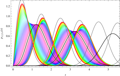
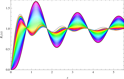
Figure 1: First four eigenvalue distributions $p_{1\sim 4}(s)$ (left) for $0.04\leq\rho\leq 0.70$ (step 0.01, purple to red) and the spectral density $R_{1}(x)$ for $0.01\leq\rho\leq 1.00$ (step 0.01) for the chGSE (black) to chGUE (grey) crossover.

Here we employ a quadrature rule consisting of a set of points $\{x_{i}\}$ taken from the interval $[0,s]$ and associated weights $\{w_{i}\}$ such that ${\int_{0}^{s}f(x)dx\simeq\sum_{i=1}^{m}f(x_{i})w_{i}}$. Similarly, the resolvents in (10) are approximated as $T_{n}(s)\simeq{\rm tr}\left(\mathbf{K}_{s}(I-\mathbf{K}_{s})^{-1}\right)^{n}.$ For a practical purpose we choose the Gauss quadrature rule, i.e. sampling $\{x_{i}\}$ from the nodes of Legendre polynomials normalized to $[0,s]$. Previously we applied the Nyström-type method to the dynamical Bessel kernels interpolating chGSE-chGUE (7) and chGOE-chGUE and evaluated the smallest eigenvalue distributions $p_{1}(s)$ [12]. In this work we extend our computation to the first four eigenvalues, aiming to reduce the fitting errors in determining the low-energy constants. We set the approximation order $m$ to be at least 100, and confirmed the stability of the results for increasing $m$ (up to $200\sim 400$).

The distributions $p_{1}(s),\cdots,p_{4}(s)$ for the $\nu=0$ case, computed from (7)$\sim$(11) for $\rho\leq 0.70$ are exhibited in Fig. 1L. A practical advantage of using individual eigenvalue distributions over the spectral density $R_{1}(x)=\sum_{k=1}^{\infty}p_{k}(x)=S(x,x)$ (Fig. 1R) for fitting the lattice data is clear from the figure: the oscillation of the latter immediately becomes structureless and insensitive to the interpolation parameter $\rho$ due to the overlapping of multiple peaks of the former, whereas the quasi-Gaussian shape of each peak is clearly distinguishable and is extremely sensitive to $\rho$. Another advantage specific to the current case originates from the fact that $p_{2k-1}(s)$ and $p_{2k}(s)$ move in opposite directions as $\rho$ is increased to break the Kramers degeneracy. By combining the two best-fitting values of $\rho$ for these two distributions, any error present in the mean level spacing $\varDelta$ of the Dirac spectrum, which would result in shifting the unfolded data of $2k-1^{\rm th}$ and $2k^{\rm th}$ eigenvalues to the same direction, is expected to be cancelled. We have confirmed this by generating $10^{5}$ samples of crossover random matrix ensembles with $N=N^{\prime}=6^{4}$ and various $\rho\leq 0.50$ and by fitting histograms of first four eigenvalues to the analytic results. Combined values of $\rho$ from these four fittings have reproduced the true input values within a few per mil of systematic error (max. 0.5%), an order of magnitude closer to the input values than using any single individual distribution. Such an accuracy could neither be hoped for had we used the spectral density $R_{1}(x)$ for fitting.

4 Effective theory and low-energy constants

The Dirac operator $D\!\!\!\!\!/$ of a QCD-like theory with quarks in a pseudoreal (real) representation, such as the fundamental of Sp$(2N)$ (SO$(N)$), possesses an antiunitary symmetry unlike QCD with quarks in a complex representation [16]: $D\!\!\!\!\!/$ commutes with ${\cal C}Z\ast$ (${\cal C}\ast$), with ${\cal C}$ being the charge conjugation and $\ast$ the complex conjugation. As $({\cal C}Z\ast)^{2}=+1$ ($({\cal C}\ast)^{2}=-1$), $D$ can be brought to a real symmetric (quaternion selfdual) matrix by a similarity transformation. Due to this property, the distinction between left-handed quarks and conjugated right-handed quarks is lost, leading to the Pauli-Gürsey extension of the flavor symmetry from ${\rm SU}(N_{F})_{L}\times{\rm SU}(N_{F})_{R}$ to ${\rm SU}(2N_{F})=:G$ and its vector subgroup from ${\rm SU}(N_{F})_{V}$ to ${\rm Sp}(2N_{F})$ or ${\rm SO}(2N_{F})=:H$. Accordingly its low-energy effective theory becomes a nonlinear $\sigma$ model on an exotic Nambu-Goldstone manifold $G/H$.

Since the Dirac operator charged under the ${\rm U(1)}$ gauge field is complex, coupling QCD-like theories with electromagnetism or even subjecting them to the constant ${\rm U(1)}$ background breaks the antiunitary symmetry of $D\!\!\!\!\!/$ and the Pauli-Gürsey extended flavor symmetry. In the latter case that is equivalent to putting on a weak imaginary chemical potential $\mu=i\mu_{I}$, its effect on the low-energy Lagrangian is systematically incorporated by the flavor covariantization of the derivatives [17]. Furthermore, if the theory is in a finite volume $V=L^{4}$ and the Thouless energy $E_{c}\simeq{{F^{2}}/{\Sigma L^{2}}}$ is much larger than $m$, the path integral is dominated by the zero-mode integration (the $\varepsilon$ regime),

$$Z=\int_{{\rm SU}(2N_{F})}\!\!\!\!\!\!\!\!\!\!\!\!\!dU\,\,\,\exp\left(\frac{1}{2}V\Sigma m\,{\rm Re}\,{\rm tr}\,\hat{M}U-V\mu_{I}^{2}F^{2}\,{\rm tr}\,(\hat{B}U^{\dagger}\hat{B}U+\hat{B}\hat{B})\right).$$ (12)

Here $U$ is an SU($2N_{F}$) matrix-valued Nambu-Goldstone field, $\hat{B}=\sigma_{3}\otimes\mathbf{1}_{N_{F}}$, $\hat{M}=i\sigma_{2}\otimes\mathbf{1}_{N_{F}}$ $\left(\sigma_{1}\otimes\mathbf{1}_{N_{F}}\right)$ for quarks in a pseudoreal (real) representation. $\Sigma=\left\langle\bar{\psi}\psi\right\rangle/N_{F}$ denotes the chiral condensate and $F$ the pseudo-scalar decay constant, both measured in the chiral and zero-chemical potential limit. Note that the above 0D $\sigma$ model for the case of fermions in a real representation can as well be derived from the random matrix ensemble (2) through the standard procedure: (i) introduce $N_{F}$ species of complex Grassmannian $(N+N^{\prime})$-vectors $\psi_{f},\bar{\psi}_{f}$ and consider a replicated spectral determinant $\left<\det(\lambda-H)^{N_{F}}\right>=\left<\int d\psi d\bar{\psi}\,{\rm e}^{\sum_{f}\bar{\psi}_{f}(\lambda-H)\psi_{f}}\right>$, where $\left<\cdots\right>$ denotes averaging over $A$ and $B$, (ii) perform Gaussian integrations over $A$ and $B$, (iii) introduce a $2N_{F}\times 2N_{F}$-matrix valued Hubbard-Stratonovich variable $Q$ and open up the 4-fermi term, (iv) perform Gaussian integrations over $\psi$ and $\bar{\psi}$, (v) take the aforementioned triple-scaling limit and denote the angular part of $Q$ (not fixed by the large-$N$ saddle point equation) as $U$. Then the coefficients of the mass and chemical-potential terms are identified as $V\Sigma m=i\pi x$ and $2VF^{2}\mu_{I}^{2}=\pi^{2}\rho^{2}$. By substituting $m\to i\lambda_{\rm Dirac}$ which turns the QCD partition function into the Dirac spectral determinant, the former equality provides the definition of unfolded Dirac eigenvalues $x=\lambda_{\rm Dirac}/\varDelta$ due to the Banks-Casher relation $\Sigma=\pi/\varDelta V$. The latter equality is used to determine $F^{2}$ from the slope of the $\mu_{I}$-$\rho$ plot.

5 Fitting Dirac spectra of SU(2)$\times$U(1) gauge theory

As the aim of this work is to demonstrate the validity and advantage of the method and not to approach the continuum, chiral, or thermodynamic limit, we chose the simplest possible setting on the lattice side: (i) generate $10^{4}$ samples of quenched SU(2)=Sp(2) gauge fields $U_{\mu}(x)$ on an (intentionally) small lattice $V=6^{4}$, with a plaquette action at $\beta_{{\rm SU(2)}}=6/g_{\rm SU(2)}^{2}=0\sim 1.75$ (step .25), using the standard heat-bath/overrelaxation algorithm. (ii-a) multiply the ${\rm SU(2)}$ fields on temporal links $U_{0}(x)$ by a constant phase ${\rm e}^{i\mu_{I}}$ with $\mu_{I}=0.00524\sim.05240$ (step .00524), or (ii-b) generate quenched noncompact ${\rm U(1)}$ gauge fields $A_{\mu}(x)$ under the Coulomb gauge-fixing condition [18] and multiply the ${\rm SU(2)}$ fields $U_{\mu}(x)$ by $\exp({ie_{{\rm U(1)}}A_{\mu}(x)})$, with $e_{{\rm U(1)}}=0.0004\sim.0024$ (step .0004), (iii) substitute the gauge fields into an unimproved staggered Dirac operator and diagonalize.

Due to the absence of the ${\cal C}$ matrix, the antiunitary symmetries of staggered Dirac operators are swapped between real and pseudoreal representations [19]. Accordingly, our case with SU(2)$\times$U(1) fundamental fermions indeed corresponds to the chGSE-chGUE crossover (2). The low-energy constants are determined by the following steps: (I) fit the histogram of each of the two smallest Dirac eigenvalues (i.e. four counting the Kramers degeneracy) of the pure SU(2) case to the rescaled chGSE ($\rho=0$) prediction $p_{k}(\lambda_{k}/\varDelta)/\varDelta$ by varying $\varDelta$, (II) combine two optimal values of $\varDelta$ and their variances to determine $\bar{\varDelta}$ and thus $\Sigma=\pi/\bar{\varDelta}V$, (III) fit the histogram of each of the four smallest unfolded Dirac eigenvalues $x_{k}=\lambda_{k}/\bar{\varDelta}$ of (a) SU(2)$+\mu_{I}$ or (b) SU(2)$\times$U(1) case to the chGSE-chGUE prediction $p_{k}(x_{k})$ by varying $\rho$, (IV) combine four optimal values of $\rho$ and their variances to determine $\bar{\rho}$ and thus $F^{2}\mu_{I}^{2}=(\pi^{2}/2)\bar{\rho}^{2}/V$.

We first observe that the four values of $\varDelta$ obtained in the step (I) are mutually consistent, giving rise to combined relative errors in $\Sigma$ that are extremely small, $\sim 0.1\%$ (Table 1, top). One-parameter fittings in the steps (I), (III-a), or (III-b) are quite satisfactory, with $\chi^{2}/{\rm dof}=0.5\sim 1.5$ for all range of parameters in concern (exemplified in Fig. 2, above). We also confirmed our expectation that the best-fitting values of $\rho$ for $k=1,3$ and those for $k=2,4$ have a tendency to counter-move, in favor of cancelling the unfolding ambiguity due to a tiny error within $\varDelta$. Relative errors in $\bar{\rho}$ are considerably reduced by the combined use of four individual eigenvalue distributions (Fig. 2 below), and are no larger than $\pm.018$(stat)$\pm.005$(sys). Linear response of $\bar{\rho}$ on $\mu_{I}$ or $e_{\rm U(1)}$ is confirmed for the SU(2)$+\mu_{I}$ case (Fig. 3, left), and the pseudo-scalar decay constant $F^{2}$ at various values of $\beta_{\rm SU(2)}$ is obtained from the slopes (Table 1, middle). For the SU(2)$\times$U(1) case, the coefficients (equivalent of $F^{2}\mu_{I}^{2}$) of the ${\rm tr}\,\hat{B}U^{\dagger}\hat{B}U$ term in (12) divided by $e_{\rm U(1)}^{2}$, extrapolated to $e_{\rm U(1)}\to 0$ are summarized in Table 1, bottom. Complete lattice results, and details of analytic and numerical computations presented in §2 and §3 will be reported in a subsequent publication.

$\beta_{\rm SU(2)}$ 0 0.25 0.50 0.75 1.00 1.25 1.50 1.75 $\Sigma\,a^{3}$ 1.310(2) 1.255(2) 1.199(1) 1.139(1) 1.070(1) .987(1) .883(1) .743(1) $F^{2}a^{2}$ .284(2) .268(2) .247(2) .226(2) .205(1) .178(1) .153(1) .115(1) $F^{2}\mu_{I}^{2}a^{4}/e_{\rm U(1)}^{2}$ 220(2) 198(2) 186(2) 163(1) 145(1) 123(1) 99.5(8) 68.0(6)

Table 1: Chiral condensate $\Sigma$ from quenched SU(2) [top], pseudo-scalar decay constant $F^{2}$ from SU(2)+$\mu_{I}$ [middle], and an equivalent of $F^{2}\mu_{I}^{2}$ (divided by $e_{\rm U(1)}^{2}$) from SU(2)$\times$U(1) [bottom], all in the lattice unit.

          

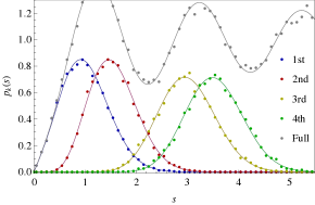
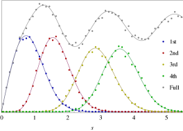
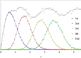
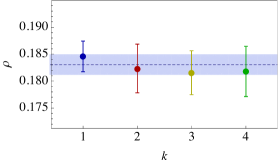
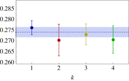
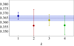
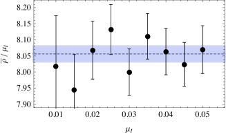
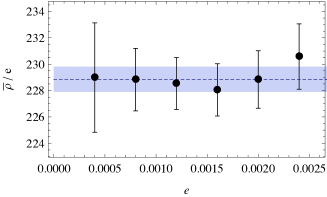
Figure 2: Histograms of $k^{\rm th}$ unfolded Dirac eigenvalues for $\beta_{\rm SU(2)}=0.25$ and $e_{\rm U(1)}=0.0008,.0012,.0016$ [above, left to right] and best-fitting $p_{k}(s)\ (k=1\sim 4)$ from the chGSE-chGUE crossover. The $\rho$ parameter determined for each $k$, their combined values [dots] and statistical errors [band] are shown below each graph.

Figure 3: Ratios $\bar{\rho}/\mu_{I}$ for SU(2)+$\mu_{I}$ at $\beta_{\rm SU(2)}=0.5$ [left] and $\bar{\rho}/e_{\rm U(1)}$ for SU(2)$\times$U(1) at $\beta_{\rm SU(2)}=0.25$ [right].

References

- [1] See e.g. M. L. Mehta, Random matrices, 3rd ed. (Elsevier, New York, 2004), Chap. 1.
- [2] O. Bohigas, M.-J. Giannoni, and C. Schmidt, Phys. Rev. Lett. 52, 1 (1984).
- [3] M. R. Zirnbauer, J. Math. Phys. 37, 4986 (1996).
- [4] S. Müller, S. Heusler, A. Altland, P. Braun, and F. Haake, New J. Phys. 11, 103025 (2009).
- [5] See e.g. K. B. Efetov, Supersymmetry in disorder and chaos (Cambridge Univ. Press, 1997).
- [6] M. V. Berry and J. P. Keating, SIAM Review 41, 236 (1999).
- [7] F. J. Dyson, J. Math. Phys. 3, 1191 (1962).
- [8] N. Dupuis and G. Montambaux, Phys. Rev. B 43, 14390 (1991).
- [9] K. Saito, T. Nagao, S. Müller, and P. Braun, J. Phys. A: Math. Theor. 42, 495101 (2009).
- [10] P. H. Damgaard, U. M. Heller, K. Splittorff, and B. Svetitsky, Phys. Rev. D 72, 091501 (2005).
- [11] P. H. Damgaard, K. Splittorff, and J. J. M. Verbaarschot, Phys. Rev. Lett. 105, 162002 (2010).
- [12] S. M. Nishigaki, Prog. Theor. Phys. 128, 1283 (2012); Phys. Rev. D 86, 114505 (2012).
- [13] P. H. Damgaard and S. M. Nishigaki, Phys. Rev. D 63, 045012 (2001).
- [14] P. J. Forrester, T. Nagao, and G. Honner, Nucl. Phys. B 553, 601 (1999).
- [15] F. Bornemann, Math. Comp. 79, 871 (2010); Markov Processes Relat. Fields 16, 803 (2010).
- [16] J. J. M. Verbaarschot, Phys. Rev. Lett. 72, 2531 (1994).
- [17] J. B. Kogut et al., Nucl. Phys. B 582, 477 (2000).
- [18] T. Blum, T. Doi, M. Hayakawa, T. Izubuchi, and N. Yamada, Phys. Rev. D 76, 114508 (2007).
- [19] M. A. Halasz and J. J. M. Verbaarschot, Phys. Rev. Lett. 74, 3920 (1995).