Halo Zeldovich model and perturbation theory:
dark matter power spectrum and correlation function

Abstract

Perturbation theory for dark matter clustering has received a lot of attention in recent years, but its convergence properties remain poorly justified and there is no successful model that works both for correlation function and for power spectrum. Here we present Halo Zeldovich approach combined with perturbation theory (HZPT), in which we use standard perturbation theory at one loop order (SPT) at very low $k$, and connect it to a version of the halo model, for which we adopt the Zeldovich approximation plus a Pade expansion of a compensated one halo term. This low $k$ matching allows us to determine the one halo term amplitude and redshift evolution, both of which are in an excellent agreement with simulations, and approximately agree with the expected value from the halo model. Our Pade expansion approach of the one halo term added to Zeldovich approximation identifies a typical halo scale averaged over the halo mass function, the halo radius scale of order of 1Mpc/h, and a much larger halo mass compensation scale, which can be determined from SPT. The model gives better than one percent accurate predictions for the correlation function above 5Mpc/h at all redshifts, without any free parameters. With three fitted Pade expansion coefficients the agreement in power spectrum is good to a percent up to $k\sim 1$h/Mpc, which can be improved to arbitrary $k$ by adding higher order terms in Pade expansion.

I Introduction

One of the major puzzles in cosmology is understanding the nonlinear formation of structure in the universe. The current state of the art are the N-body simulations, which have been verified to give reliable answers at 1% level in the power spectrum up to $k\sim 1$h/Mpc Heitmann et al. (2010), but are expensive to run, require large allocations, and are often not fully convergent using typical current generation box size and resolution. The convergence properties become a lot more difficult to achieve for higher order correlations. For example, recent studies have shown that to reach one percent convergence on the covariance matrix one needs to simulate a volume in excess of 1000${\rm Gpc^{3}}$ Blot et al. (2014), and the covariance matrix depends both on the cosmological model and on the size of the survey one is simulating, making the numerical solution to the full problem an excessively demanding task given the current typical resources. Even more importantly, we want to use clustering statistics to extract information about our universe, and simulations do not provide much insight to the questions such as where is the information content and how to optimally extract it from the data.

Alternative approach is to use perturbation theory (PT), of which the two most prominent examples are standard PT (SPT) and Lagrangian PT (LPT) (see Bernardeau et al. (2002) for a review). In this approach one assumes density perturbation is less than unity, and one expands the nonlinear equations perturbatively. Since density perturbations grow with wavevector $k$, this approach breaks down for some $k>k_{\rm nl}$. The current approaches typically underpredict power in LPT and overpredict in one loop SPT. For example, we know that Zeldovich approximation is quite successful in modeling the correlation function on large scales, including the baryonic acoustic oscillations (BAO) wiggles White (2014). However, it fails miserably in the power spectrum, underestimating the power at all but the lowest values of $k$, and giving predictions that are even below the linear theory at $z=0$ Vlah et al. (2015). Various one loop LPT extensions (one loop LPT Matsubara (2008), CLPT Carlson et al. (2013), CLPTs Vlah et al. (2015)) somewhat improve this for the power spectrum, but make things worse for the correlation function Vlah et al. (2015). Physically, the problem of Zeldovich approximation and its extensions is that while it can describe properly the initial streaming of dark matter particles, it fails to account for their capture into the dark matter halos: instead, the particles continue to stream along their trajectories, set by initial velocity in Zeldovich approximation, leading to an excessive smoothing of the power.

Standard Eulerian PT (SPT) has the opposite problem. In power spectrum it quickly overpredicts the amount of power at one loop level, specially at low redshifts. The reason for this is that the loop integrals extend over all modes, including those that are in the nonlinear regime $k>k_{\rm nl}$. These modes are not in PT regime and typically these contrubutions are strongly suppressed in the simulations relative to PT, leading to too much power in SPT relative to simulations. Its Fourier transform, using a gaussian smoothing to obtain a convergent correlation function, results in a worse model than the Zeldovich approximation around BAO, but is otherwise comparable. Recent work emphasized this point in the context of effective field theory (EFT) Carrasco et al. (2012). For example, for power law power spectra these integrals can be divergent, so PT is wrong in such situations Pajer and Zaldarriaga (2013). Instead, it is argued that the best that one can do is to introduce effective field theory parameters that describe the correction from the small scale physics. For $k<1/R_{h}$ these terms can be expressed as a low $k$ limit of PT, but with free parameters. A priori it is unclear what is $R_{h}$, and how large these corrections are for our universe. In particular, realistic CDM power spectra have the shape where most of the low $k$ limit loop integral comes from scales in the linear regime, where PT is believed to be valid, making the corrections from the nonlinear scales small, although probably not negligible. We will try to quantify this in more detail below. We will argue that halo model requires $R_{h}$ to be a typical halo radius.

The philosophy we will advocate in this paper is that any analytic approach must give reliable results both in Fourier and in configuration space. Failure to do so is a sign of something missing in the model. For example, a Taylor series may give reliable results in Fourier space up to a certain $k$, but if truncated at a certain order it generally diverges at high $k$ and makes its Fourier transform imposible to calculate. The reason is that the series is not convergent at high $k$, and one has to adopt a different summation of the terms that have a better convergence. Our goal is to develop a model that is rooted in PT as much as possible, but is also able to reproduce simulations. Since simulations have been verified at 1%, we will strive for this precision in this paper.

II Halo Zeldovich model and Perturbation Theory

The main ingredients of our approach are the following:

1) 1 loop SPT has loop integrals which, for low $k$ and high $z$, are entirely in the linear regime and thus reliably computed. There is no guarantee that the entire loop integral is correct at all redshifts, even for low $k$, but we will make this assumption here and derive the consequences. We will therefore assume that EFT corrections to 1 loop SPT are negligible at low $k$. For higher $k$ and low $z$ SPT predictions become increasingly unreliable and will not be used. Similarly, 2 loop SPT integrals are negligible at high $z$, while for low $z$ they extend deeply into the nonlinear regime and are grossly overestimated in SPT Vlah et al. (2015). Here we will simply ignore 2-loop SPT, with one exception, discussed next.

2) Zeldovich approximation gives approximately correct physical picture of how the particles are displaced up to the process of halo formation, which stops the particles from displacing. The latter has very little effect on the Zeldovich displacement: most of the displacement is generated by modes in the linear regime and we will not be correcting Zeldovich approximation. In terms of SPT Zeldovich approximation receives contributions from loops at all order, but only from very specific terms related to the linear displacement field correlation function.

3) Halo formation has to be an essential part of the complete model. Halos are objects of very high density, leading to a nearly white noise like contribution to the power spectrum at low $k$, with the halo profile parameters determining deviations from white noise at higher $k$. At high $k$, the halo term contribution dominates the correlations: all of the close pairs are inside the same halos. At a scale $k\sim 1/2R_{\rm vir}$ the number of close pairs involves all of the pairs inside the virial radius, which must give a contribution of the other of $M^{2}$, where $M$ is the virial mass of the halo. Integrating over all the halos, and weighting by the halo mass function $dn/dM$, one obtains an estimate of one halo amplitude $\bar{\rho}^{-2}\int M^{2}(dn/dM)dM$, where $\bar{\rho}$ is the mean density of the universe. At redshift 0 the integral is dominated by cluster mass halos with virial radius of 1-2${\rm h^{-1}Mpc}$. We expect the one halo term to be approximately of this amplitude at $k\sim 0.2-0.4{\rm h/Mpc}$. However, the mass has to be conserved so the halos have to be compensated, which forces the one halo term to vanish at very low $k$. There is no unique way to do this, since it depends on what we compensate against. The compensation is by definition a two halo term, since the mass is being compensated by the particles outside the virial radius. Here we compensate against Zeldovich and demand that the total agrees with SPT, which then automatically enforces mass and momentum conservation.

4) More specifically, we will assume that 1) can be connected to 2) and 3) at some low $k$, which is low enough that SPT can be assumed to be valid, yet large enough to still be close to the scale which dominates the compensation. We will match the two on this scale where both descriptions are valid, and use 2)+3) at higher $k$. Since we believe that Zeldovich approximation is a good starting point for any modeling we will include it as one ingredient of the theory, and decompose the power spectrum and correlation function into two parts,

$$P(k)=P_{\rm{Zel}}+P_{BB},\,\,\,\,\xi(r)=\xi_{\rm{Zel}}(r)+\xi_{BB}(r).$$ (1)

Here subscript $Zel$ stands for Zeldovich and $BB$ for broadband beyond Zeldovich Vlah et al. (2015), which is our one halo term. While there may be a residual BAO wiggle signature that is not captured by Zeldovich, it is essentially negligible in the power spectrum and at most a few percent in the correlation function around BAO (100Mpc/h), probably too small to be observed by existing or future redshift surveys due to large sampling variance errors. Here we will thus focus on the modeling of the broadband one halo component and ignore the wiggle part. Note that we do not assume that the Zeldovich part is uncorrelated with the one halo term. In this sense our one halo term is not the so called stochastic term uncorrelated with Zeldovich.

As we argued the key physics ingredient missing in PT is the halo formation, which leads to a large contribution from the near zero lag correlations, also called the one halo term in the halo model Seljak (2000); Peacock and Smith (2000); Ma and Fry (2000); Cooray and Sheth (2002). The halo model postulates that the nonlinear evolution leads to halo formation, and that all the dark matter particles belong to collapsed halos, with the halo mass distribution given by the halo mass function $dn(M)$. The correlations between the dark matter particles can be simply split into correlations within the same halo, the one halo term, and between halos, the two halo term. On large scales the latter reduces to linear theory $P_{L}(k)$. The one halo term in the halo model has a simple physical interpretation on small scales, which is that all dark matter particles are inside the dark matter halos distributed with a radial halo density profile, and this leads to a power spectrum that is simply an integral over the halo mass function times the Fourier transform of the halo profile squared. The halo profile has a compact support, extending out to roughly the virial radius, and its correlation function is a convolution of the profile with itself, extending to roughly twice that. In power spectrum the convolution becomes a square of the Fourier transform of the profile, which can be expanded as a series of even powers of $k$ Mohammed and Seljak (2014),

$$P_{BB}(k)=F(k)A_{0}\left(1-R_{1h,2}^{2}k^{2}+R_{1h,4}^{4}k^{4}+...\right).$$ (2)

Here the parameters $A_{0}R_{1h,n}$ have a specific interpretation in terms of the integrals over the halo mass function $n(M)$ times halo mass $M$ squared, and times $2n$ moments of the halo radius averaged over the halo density profile Mohammed and Seljak (2014). Specifically, $A_{0}=\bar{\rho}^{-2}\int M^{2}dn(M)$ is just a weighted halo mass squared divided by the mean density $\bar{\rho}$ and does not depend on the halo density profile. These arguments however do not yet account for the halo compensation. Above we introduced $F(k)$, which is the compensation function, required to vanish in $k\rightarrow 0$ limit as long as the two halo term converges to linear theory in the same limit: mass conservation requires that the leading nonlinear one halo term cannot be a constant $A_{0}$ Mohammed and Seljak (2014). Thus one halo term has to be generalized to include mass compensation effects: nonlinear effects cause the dark matter to collapse into dark matter halos, bringing in mass from larger scales, so it has to be compensated by a mass deficit at large scales to satisfy the mass (and momentum) conservation. Because of this one can show that the one halo term has to scale as $k^{4}$ at low $k$ Peebles (1993); Seljak (2000); Valageas et al. (2013).

The two halo term can also be expressed as a convolution of the linear theory over the halo profiles, and the resulting Taylor expansion is given by a similar series

$$P_{2h}(k)=P_{L}(k)\left(1-k^{2}R_{2h,2}^{2}+k^{4}R_{2h,4}^{4}...\right).$$ (3)

The leading order correction scales as $k^{2}P_{L}(k)R_{2h,2}^{2}$, where $R_{2h,2}$ is also related to an average second moment of halo density profile, although with a different mass and halo bias weighting Seljak (2000). Note that this gives at the leading order correction the usual EFT term Carrasco et al. (2012). It is clear that both one halo and two halo Taylor expansions break down for $k>R_{h,2}^{-1}$. The breakdown of the two halo term does not matter: at the relevant $k$ the correlations are dominated by the one halo term. For the latter however, a different expansion is advantageous, as we discuss below.

In this paper we argue that the natural way to connect SPT to small scale nonlinear effects is in the context of the Zeldovich approximation plus a compensated one halo term. In this picture we can think of $P_{\rm{Zel}}$ as the leading order two halo term, and $P_{BB}$ as the one halo term. The motivation for this is that Zeldovich correlation function is almost exact for $r>5Mpc/h$, and that the correction relative to it is negative, suggesting a compensation of a nonlinear term $\xi_{BB}(r)$. All the corrections to the Zeldovich model thus go into the compensation term $F(k)$. In the halo model these corrections would arise from compensation of the halo term and from two halo term correlations of particles inside the halos. We do not try to separate these into the latter that one expects to scale as $k^{2}P_{L}(k)$ at low $k$, and the former that scales as $k^{4}$ at very low $k$. In general it is difficult to do this separation, as both of these arise from the two halo term correlations. It is also not clear that in the regime where it matters ($k>0.1h/Mpc$) these low $k$ expansions still apply. We will however use them at very low $k\sim 0.02h/Mpc$, where we expect SPT to be valid. However, it should be clear that the term $P_{BB}$ is not just the one halo term in the traditional sense, because of these compensation corrections at low $k$.

In Mohammed and Seljak (2014) this function $F(k)$ was simply fitted using a polynomial form. We will begin by keeping this function completely general, and then choosing a very simple form for it. Our one halo term, and thus the compensation form of $F(k)$, is defined relative to the Zeldovich term. If we adopted a different form for the two halo term we would obtain a different form of $F(k)$. In principle, Zeldovich approximation itself could contain some halos with correct mass and so a part of what we usually call one halo term could already be contained there. However, we will see that this must be a minor effect and the one halo term we derive agrees with the expected value from the halo model.

While the one halo expansion in even powers of $k$ above works in Fourier space up to the virial radius scale of order $k\sim R_{1h,2}^{-1}\sim 1$h/Mpc, it breaks down above that. Moreover, powers of $k$ diverge at high $k$ and do not have a well defined Fourier transform, making this form unsuitable for correlation function predictions without resumming it first. Instead we will use in this paper the Pade series ansatz

$$P_{BB}=A_{0}F(k){1+\sum_{m=1}^{n_{\rm max}-1}(kR_{m})^{2m}\over 1+\sum_{n=1}^{n_{\rm max}}(kR_{nh})^{2n}}.$$ (4)

By requiring the series in the denominator to run to a higher power than in the enumerator we guarantee that the series does not diverge at high $k$ and has a finite Fourier transform. Here we will explore the truncation of the series at $n_{\rm max}=0,1,2$. In terms of the halo model $A_{0}$ has the same interpretation as before, it is the halo mass mass squared averaged over the halo mass function. It is the only quantity that has units of power spectrum, all the other parameters have units of length. For the $R_{m}$ and $R_{nh}$ parameters we expect that they will be related to a typical scale of the halos. There are several halo scales one can define: one is the scale radius $R_{s}$, defined as the scale where the slope of the density profile is -2. Another scale we can define is the virial radius $R_{\rm vir}=cR_{s}$, where $c$ is the concentration parameter with values around 3-4 for the most massive halos and increasing towards less massive halos Navarro et al. (1997). The mean overdensity at $R_{\rm vir}$ is 200 by definition, while the typical mean overdensity at $R_{s}$ can be of order 1000 or more. In the halo model approach we integrate over these with the halo mass function, and the number of pairs for each is proportional to $M^{2}$, which gives most of the weight to the very massive halos. As a result, if we use $n_{\rm max}=1$ and only have one scale parameter, which we denote $R^{0}_{h1}$, then we find that the typical scale, when averaged over all halos, is of order 1Mpc/h at $z=0$, a typical scale of a cluster.

While the halo model has been successful as a phenomenological model, its connection and consistency with PT has not been explored. In this paper we propose a Halo Zeldovich model applied to Perturbation Theory (HZPT) approach, in which we connect the halo model to PT in the regime where both can be expected to be approximately valid. We take the approach that one loop SPT has a regime of validity on very large scales and gives us the correct description of the onset of nonlinearity. This is not guaranteed by SPT: the one loop SPT may receive contributions from small scales which are nonlinear and thus not reliably computed. For CDM type power spectra, the integrals are convergent and for sufficiently high redshift all of the one loop integral contributions come from linear scales, the prediction is reliable, and no EFT correction is needed. For now we will simply assume there are no corrections to SPT at low $k$, and return to this discussion later.

Let us therefore assume that one loop SPT is correct at very low $k$, and that it can be matched to the halo model ansatz in equation in the regime of its validity. The low $k$ limit of Zeldovich approximation is Vlah et al. (2015) $P_{\rm Zel}=(1-k^{2}\sigma_{L}^{2}+k^{4}\sigma_{L}^{4}/2)P_{L}+Q_{3}/2$, where $P_{L}$ is the linear power spectrum, $\sigma_{L}^{2}=1/(6\pi^{2})\int dqP(q)$ is the square of linear displacement field dispersion and $Q_{3}=1/(10\pi^{2})k^{4}\int dqP^{2}(q)/q^{2}=C_{3}k^{4}$ is a mode coupling integral, as defined in Matsubara (2008). It has been shown in Vlah et al. (2015) that this expansion is valid for $k<0.1$h/Mpc. Note that we kept terms beyond 1-loop in the Zeldovich. One loop SPT can be written as $P_{\rm SPT}=P_{L}+P_{13}+P_{22}$, which at low $k$ is $P_{13}=-61/105k^{2}\sigma_{L}^{2}P_{L}$ and $P_{22}=45Q_{3}/98$.

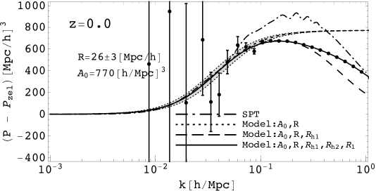
Figure 1: HZPT model for $n_{\rm max}=0,1,2$ (dotted, dashed and solid lines respectively), together with SPT (dot-dashed line) are shown as a function of $k$. We match SPT to HZPT around $k\sim 0.02$h/Mpc to derive $A_{0}$ and $R$, while the remaining parameters of our model ($R_{1}$, $R_{1h}$, $R_{2h}$) are fitted to simulations (points) at scales $k>0.1$h/Mpc. Gray band shows the change in the HZPT, $n_{\rm max}=0$ model in case where $R$ value varies for $\pm 3$Mpc/h. This plot is for $z=0$, and higher $z$ versions are similar. Simulation points are taken from Vlah et al. (2015), and are for $\sigma_{8}=0.807$ Lambda CDM model.

Let us begin by first dropping the 2-loop term $k^{4}\sigma_{L}^{4}P_{L}/2$ from Zeldovich approximation. Then all of the one loop terms scale as the square of the power spectrum. Matching at low $k$ gives

$$P_{\rm SPT}(k)-P_{\rm{Zel}}(k)={44\over 105}k^{2}\sigma_{L}^{2}P_{L}-{2\over 49}Q_{3}=A_{0}F(k),$$ (5)

where the linear order cancels in the difference and we have dropped all higher order terms since they are negligible at low $k$. What does this imply for the amplitude dependence of $A_{0}$ and $F(k)$? We will adopt the standard $\sigma_{8}$ normalization for the amplitude of fluctuations, where $\sigma_{8}(z)$ is the rms fluctuation of spheres of radius of 8Mpc/h, and which is redshift dependent. Often this is phrased in terms of the redshift dependence of the growth factor $D(z)$, and in linear theory we would write $\sigma_{8}(z)=D(z)\sigma_{8}(z=0)$. But the amplitude dependence is more general than the redshift dependence, since it encompases the idea that changing the redshift or changing the amplitude should give the same result in the context of PT. Since both SPT and Zeldovich at low $k$ scale as a square of the power spectrum, which itself scales as $\sigma_{8}^{2}$, requiring equation 5 to be valid over a broad range of $k$ where $F(k)$ is rapidly changing, there can only be one solution to the amplitude dependence, $A_{0}\propto\sigma_{8}^{4}$ and $F(k)={\rm const}$. This simple result is in very close agreement with simulations spanning a wide range of redshifts and models Mohammed and Seljak (2014), where the slope of 3.9 was derived. We will see below that including the full Zeldovich instead of its lowest order further improves the agreement on the slope. Note that this is valid for a general compensation function $F(k)$.

To proceed we need to assume a specific functional form for the compensation term. A simple way to achieve compensation is to use $F(k)=1-1/(1+k^{2}R^{2})$, which has an analytic Fourier transform and vanishes as $k\rightarrow 0$, so that the overall model for one halo term is

$$P_{BB}=A_{0}\left(1-{1\over 1+k^{2}R^{2}}\right){1+\sum_{m=1}^{n_{\rm max}-1}(kR_{m})^{2m}\over 1+\sum_{n=1}^{n_{\rm max}}(kR_{nh})^{2n}}.$$ (6)

The parameter $R$ governs the transition of the one halo term to 0 at low $k$: this is the compensation scale parameter, and we expect it to be very large compared to the typical halo size. Here we simply chose the simplest form for this function $F(k)=(1-1/(1+k^{2}R^{2})$, but we do not expect this to be the correct form at all $k$, since, as seen from equation 5, the residual between SPT and Zeldovich at low $k$ is not $k^{2}$, but $k^{2}P_{L}$. We evaluate SPT and Zeldovich in the low $k$ limit and fit for parameters $A_{0}$ and $R$. We find there is a range of $k$ where the fit is good (figure 1) and we use $0.02{\rm h/Mpc}<k<0.05{\rm h/Mpc}$ for the fits. The fit is not perfect, a consequence of the simplified form of $F(k)$ term, but is a good fit for $0.02{\rm h/Mpc}<k<0.05{\rm h/Mpc}$. Even for the more general forms of $F(k)$ one can still define a typical compensation scale on which $F(k)$ goes from unity to zero. Current form of compensation is sufficient for our purposes and we will not explore more general forms. We find

$$A_{0} = 750\left({\sigma_{8}(z)\over 0.8}\right)^{3.75}\text{(h/Mpc)}^{3}$$

$$R = 26.0\left({\sigma_{8}(z)\over 0.8}\right)^{0.15}\text{(Mpc/h)}$$ (7)

This is a remarkably simple result. Moreover, it agrees well with the recent numerical determination of $A_{0}$ amplitude from a suite of 38 emulator simulations at different redshifts in Mohammed and Seljak (2014), where a scaling $A_{0}=670(\sigma_{8}/0.8)^{3.9}({\rm Mpc/h})^{3}$ has been derived over the redshift range 0-1. The amplitude is a bit different because the form of compensation used in this letter is a bit different than in Mohammed and Seljak (2014), but they both provide equally good fit to the simulations, as shown in figure 1. The two parameters are correlated, and parameter $R$ is less well determined than $A_{0}$: $R$ comes with five times larger relative error than the error on $A_{0}$. Figure 1 shows the band over which $R$ is varied by 12%: a reasonable estimate of its error is 3-5% (and the error on $A_{0}$ is 1% or less). We find the slopes of $A_{0}$ and $R$ to be uncertain at 0.1 level. The value of the amplitude also agrees very well with the expected amplitude of the one halo term in the halo model, which is $\bar{\rho}^{-2}\int M^{2}dn$, where $M$ is the halo mass, $dn/dM$ is the halo mass function and $\bar{\rho}$ is the mean density of the universe. This suggests that Zeldovich approximation on itself does not contribute much to the one halo term.

To qualitatively derive a value for $R$ and $A_{0}$ let us look at the low $k$ limit of SPT, focusing on the leading order $k^{2}$ and $k^{4}$ terms at the peak of the power spectrum around $k_{\rm peak}\sim 0.02$h/Mpc, where $P_{L}(k_{\rm peak})\sim 27000(\sigma_{8}/0.8)^{2}{\rm(h/Mpc)^{3}}$ and $\sigma_{L}^{2}\sim 36(\sigma_{8}/0.8)^{2}({\rm Mpc/h})^{2}$. Since the difference between Zeldovich and SPT for the low $k$ gives $(44/105)k^{2}\sigma_{L}^{2}P_{L}$, by equating that to $k^{2}A_{0}R^{2}$ (low $k$ limit of equation 5) we derive $R\sim(0.42\sigma_{L}^{2}P_{L}(k_{\rm peak})/A_{0})^{1/2}\sim 24$Mpc/h for the best fit value of $A_{0}$, in a qualitatively good agreement with the value of 26Mpc/h derived numerically. Thus the value of $R$ is determined by the linear power spectrum amplitude at the peak, rms displacement field and the amplitude of the one halo term $A_{0}$. To determine both $A_{0}$ and $R$ we need to expand SPT and Zeldovich up to $k^{4}$ around $P_{L}(k_{\rm peak})$, for which we also need to numerically evaluate $C_{3}\sim 2\times 10^{9}{\rm Mpc/h}$. Matching $k^{4}$ terms gives $[(1/2-45/98)C_{3}+(\sigma_{L}^{2})^{2}P_{L}/2]=A_{0}R^{4}$, which, when combined with $k^{2}$ term gives $R\sim 20$Mpc/h and $A_{0}\sim 700({\rm Mpc/h})^{3}$ at $z=0$. We note further that there is a considerable contribution beyond $k^{4}$ from $P_{13}$ already around $k\sim 0.02{\rm h/Mpc}$, and in the numerical fits there is some correlation between $A_{0}$ and $R$.

The Zeldovich term beyond 1-loop, $(\sigma_{L}^{2})^{2}P_{L}/2$, cannot be neglected compared to the rest of $k^{4}$ terms even for $k<0.05{\rm h/Mpc}$, and as a consequence the scaling of $A_{0}\propto\sigma_{8}^{4}$ and $R={\rm const}$ is mildly broken. This term is larger for low redshifts, explaining why the slope of $\sigma_{8}$ scaling is less than 4.0 and closer to 3.8. Remarkably, that is exactly what simulations suggest. Given the uncertainties in the form of $F(k)$ we cannot address in detail the remarkably small scatter of $A_{0}$ against the amplitude $\sigma_{11.3}$ when the shape of the power spectrum is varied Mohammed and Seljak (2014).

The leading order for our compensation term of the one halo $F(k)$ is $k^{2}$. It is often stated that the mass and momentum conservation effects generate $k^{4}$ tail Crocce and Scoccimarro (2008), and so one would naively expect the leading term of one halo to be $k^{4}$. This term is generated by $P_{22}$ in SPT. However, nonlinear evolution also leads to propagator effects contained in $P_{13}$, which at the leading order give $k^{2}P_{L}$ corrections to the linear theory and we have seen that these effects dominate at low $k$. We have assumed the two halo term to be Zeldovich approximation, which contains part of the $k^{2}P_{L}$ term in SPT but not all, and so the difference is still given by $k^{2}P_{L}$ term at the leading order, which has to be the leading order one halo term, and happens to coincide with $k^{2}$ at the peak of the power spectrum around $k\sim 0.02$h/Mpc, where we fit to our ansatz. As discussed above, we could use a more general form of $F(k)$ that would make the compensation and two halo terms exact, but we found this makes no practical difference to the final results. It is also possible to make a different two halo ansatz where $k^{2}P_{L}$ is entirely cancelled, for example, our two halo ansatz could be simply $P_{13}$ of SPT, or its nonlinear propagator version Crocce and Scoccimarro (2008). As shown in Crocce and Scoccimarro (2008), this ansatz leads to one halo term that is several times larger than expected in the halo model. It is possible to generate a valid halo model based on a different ansatz for the two halo term, but we do not pursue this further here.

III Power spectrum predictions of HZPT

In this section we fit higher order parameters of the one halo term to obtain the best possible agreement against simulations. The best fits for these parameters as powers of amplitude $\sigma_{8}(z)$ give

$$R^{0}_{1h} = 1.87{\rm Mpc/h}\left({\sigma_{8}(z)\over 0.8}\right)^{-0.47},$$

$$R_{1h} = 3.87{\rm Mpc/h}\left({\sigma_{8}(z)\over 0.8}\right)^{0.29},$$

$$R_{1} = 3.33{\rm Mpc/h}{\sigma_{8}(z)\over 0.8}^{0.88},$$

$$R_{2h} = 1.69{\rm Mpc/h}\left({\sigma_{8}(z)\over 0.8}\right)^{0.43}.$$ (8)

Here $R^{0}_{1h}$ refers to $n_{\rm max}=1$ case, while $R_{1h}$, $R_{2h}$ and $R_{1}$ refer to $n_{\rm max}=2$ case. Even though we only fit to one set of simulations, we expect that these parameters are nearly universal and apply well to all cosmological models, just as in the case of the halo plus Zeldovich model of Mohammed and Seljak (2014). The main difference relative to Mohammed and Seljak (2014) is the form of the compensation function $F(k)$, which was fitted to a 10-th order polynomial in Mohammed and Seljak (2014), while here we adopt a much simpler form of equation 6, and the expansion of the one halo term, which was in even powers of $k$ in Mohammed and Seljak (2014), while we use Pade expansion here.

In figure 2 we show the HZPT for $P(k)$ against the N-body simulations for four different redshifts. We find that the model with $n_{\rm max}=1$ can fit the simulations at 1% up to $k\sim 0.3$h/Mpc, while for $n_{\rm max}=2$ the fits are good to 1% up to $k\sim 1$h/Mpc. Parameter $R$ ensures the low k behaviour of the model, while $A_{0}$ sets the peak amplitude of $P_{BB}$ which is around $k\sim 0.12$h/Mpc for all redshifts. In Jeong and Komatsu (2006) has been argued that SPT is a relatively good description against N-body simulations for $z>3$. This is consistent with our results: as shown in figure 2, for $z=2$ SPT differs from simulations by only 2%, and this difference is presumably even smaller for higher $z$.

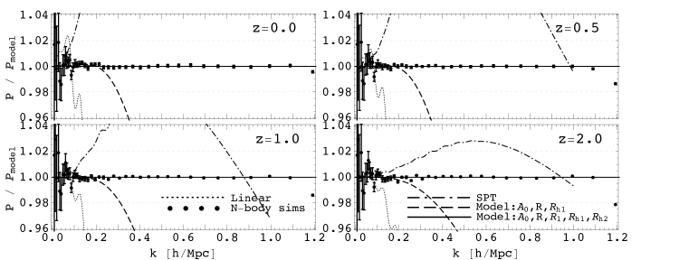
Figure 2: Simulation power spectrum (points) is shown relative to HZPT model prediction ($P_{\rm model}$) with $n_{\rm max}=2$ (black solid line) at four different redshifts ($z=0.0$, $0.5$, $1.0$ and $2.0$). Also shown are SPT (dot-dashed line), HZPT with $n_{\rm max}=1$ (dashed line) and linear theory (dotted line). Simulation points are taken from Vlah et al. (2015), and are for $\sigma_{8}=0.807$ Lambda CDM model.

We have established that one loop SPT can determine $A_{0}$ and $R$. Which other coefficients of equation 6 can PT determine? Since coefficients $R_{nh}$, $R_{n}$, $n>0$, are determined by a typical halo scale averaged over the halo profile and averaged over the halo mass function, they depend on the regime where the overdensity is very large: halo virial radius $R_{\rm vir}$ is defined at a mean overdensity of 200, and $R_{s}$ is even smaller (with the correspondingly larger mean overdensity). These cannot be computed from standard PT, which is only supposed to work in the regime where $\delta<1$. One can show (figure 2) that these terms become important at a percent level around $k\sim 0.2$h/Mpc at $z=0$. It seems unlikely that PT can make predictions at a percent level for $k>0.2{\rm h/Mpc}$, regardless of which PT formalism we use. It is however remarkable that one loop SPT can predict the amplitude of the one halo term $A_{0}$. This is possible because $A_{0}$ depends on the total halo mass that has nonlinearly collapsed and not on its profile. At low $k$ the non-perturbative halo profile effects also give rise to the two halo correction term of order $k^{2}R_{2h}^{2}P_{L}$, where $R_{2h}\sim 1$Mpc/h. This is the EFT term of Carrasco et al. (2012). At low $k$ this term is a small, a few percent, correction to the SPT term, which is of course small compared to linear theory. At higher $k$ this term is modified and in our model absorbed into the overall compensated one halo term $P_{BB}$.

IV Correlation function predictions of HZPT

We would like to require from a good PT model that it works both in Fourier and in configuration space, but so far there has been no successful model achieving this. Typically, Zeldovich approximation works quite well in correlation function but fails in the power spectrum, while SPT does not give very good correlation function predictions, specially around BAO. In HZPT approach, we expect Zeldovich term to dominate the correlation function at large radii. In the absence of compensation the one halo term would be limited to scales around twice the virial radius and below. With compensation these effects extend to large radii, but as we will show, remain small. There is thus a crucial difference of the effect of the one halo term between correlation function and power spectrum: the one halo term is mostly a few percent effect for $r>5{\rm Mpc/h}$ in correlation function, caused by compensation effects. On the other hand, one halo term can be very large for $k>1/R\sim 0.04{\rm h/Mpc}$ in the power spectrum and dominates $P(k)$ for $k>0.2{\rm h/Mpc}$.

An advantage of the ansatz in equation 6 is the existence of analytical Fourier transform for low $n_{\rm max}$. On scales $r\gg R_{\rm halo}$, and assuming $R\gg R_{nh},R_{n}$, one can use $n_{\rm max}=0$ and find

$$\xi_{BB}(r)=-\frac{A_{0}e^{-\frac{r}{R}}}{4\pi rR^{2}}.$$ (9)

Similarly, if we keep the leading $R_{h1}$ effects in $n_{\rm max}=1$ case we get:

$$\xi_{BB}(r)=-\frac{A_{0}e^{-\frac{r}{R}}}{4\pi rR^{2}}\left(1-\left(\frac{R}{R_{h1}}\right)^{2}\exp\left[-\frac{R+R_{h1}}{RR_{h1}}r\right]\right).$$ (10)

First equation effectively reduces the low $k$ model that we started with in Fourier space to a model in the configuration space with the same two parameters, $A_{0}$ and $R$, that have been determined using SPT. Since the virial radius of the largest halos is about 2Mpc/h at $z=0$, we expect the transition between the two regimes to be around 4Mpc/h. The results for the correlation function are shown in figure 3. We see that our model significantly improves upon other PT results, achieving 1-2% agreement down to 5Mpc/h at all redshifts. A possible exception is the BAO wiggle, r$>$80Mpc/h, where there may be additional wiggle contribution that was discussed in Vlah et al. (2015), but it is unclear whether it is real given the large sampling variance fluctuations. It also improves upon Zeldovich approximation, which is already very good by itself, with only a few percent deviations from simulations over this range. Our model reduces the correlation function relative to Zeldovich, as expected by the compensation effects, which take mass from large scales to enhance one halo terms on small scales. As expected our resuts agree with SPT on large scales, but only away from BAO, making the range where SPT agrees with simulations and our model at 1% level only around 50-70Mpc/h.

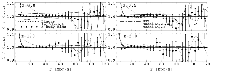
Figure 3: Simulation correlation function (points) is shown relative to HZPT model prediction ($\xi_{\rm model}$) with $n_{\rm max}=0$ (black solid line) at four different redshifts ($z=0.0$, $0.5$, $1.0$ and $2.0$). Note that HZPT $\xi_{\rm model}$ with $n_{\rm max}=0$ if completely determined with the $A_{0}$ and $R$ parameters obtained from the low $k$ of SPT power spectrum. Also shown are HZPT with $n_{\rm max}=1$ (dashed line), Zeldovich (long dashed line), SPT (dot-dashed line), and linear theory (dotted line). Simulation points are taken from Vlah et al. (2015), and are for $\sigma_{8}=0.807$ Lambda CDM model.

Given that the one halo contribution relative to Zeldovich is a few percent only, any further corrections have a very small effect on $\xi(r)$ for $r>5{\rm Mpc/h}$. For example, one can improve the agreement of the model with simulations somewhat by increasing $R$. We can do this at a few percent level since this is the formal error from the fits to SPT. In the context of our approach, increasing $R$ beyond its SPT predicted value at a level more than this would only be possible if there are nonperturbative or 2-loop corrections at low $k$, since an assumption of our model is that one loop SPT is the correct theory at low $k$. Note that EFT corrections as advocated by Carrasco et al. (2012) will reduce $A_{0}R^{2}$, which goes in the opposite direction. Nevertheless, as discussed above, there is no guarantee for SPT to be true even for very low $k$: the loop integrals can extend into the regime where density perturbation exceeds unity. At $z=0$, for CDM models, this happens around $k_{\rm nl}\sim 0.1-0.2$h/Mpc. The low $k$ expansion of SPT is dominated by $k^{2}\sigma_{L}^{2}P_{\rm lin}(k)$ terms, which depend only on the convergence of the $\sigma_{L}^{2}$ integrals. This converges to about 90% of the value for $q\lesssim k_{\rm nl}\sim 0.2$h/Mpc at $z=0$, and converges even more to its full value for $z>0$ where $k_{\rm nl}>0.2$h/Mpc Vlah et al. (2015). So we expect the one loop SPT to be almost perfectly valid at low $k$ for high redshifts, but there may be low redshift corrections at a several percent level, which may allow for additional changes in $R$ or $A_{0}$ beyond the predicted value at at comparable level. In addition, our form of the compensation term is just an assumed ansatz, which could be modified for a better agreement.

A related question is whether one should include higher loop contributions. At a next order in PT is the two loop SPT or, similarly (although not equivalently), one loop LPT. In both cases the corrections to one loop SPT can become important at low redshifts, even at low $k$. For example, at $z=0$ the two loop SPT correction to $P_{13}$ is about 15% Vlah et al. (2015), and since the relative correction of two loop to one loop scales as $\sigma^{2}_{8}$, the correction is much smaller at higher redshifts. However, higher loop contributions are likely to be grossly overestimated in PT. For example, comparison against simulations suggests that the one loop LPT contribution to rms displacement is in reality almost entirely suppressed, such that the total nonlinear value of $\sigma_{NL}^{2}$ differs by only 1-2% relative to the linear value $\sigma_{L}^{2}$ at all redshifts Chan (2014); Tassev (2014); Vlah et al. (2015). Physically this can be understood by the process of halo formation, which stops particles from displacing on small scales, and instead traps them inside the dark matter halos: the large scale displacements, which are one loop in SPT, are correctly predicted, while the small scale displacements, two loop and higher in SPT sense, are strongly suppressed. It thus seems better to drop two loop terms entirely, although we have no formal proof of this statement.

In summary, formally one cannot exclude corrections at low $k$, which will be of the EFT form $k^{2}P_{L}$, but these are likely to be of order a few percent only. We see no need for such corrections in our approach: our model is accurate at the current precision of simulations. We thus argue that one loop SPT is close to the correct theory for $k<R^{-1}$, but this is not a result that can be formally derived.

V Conclusions

In this paper we develop a model for dark matter power spectrum and correlation function that is 1% accurate for both, and that is based on perturbation theory (PT) as much as possible. We argue that PT approaches to large scale structure can only have a hope of being valid for very large scales, $k<0.05{\rm h/Mpc}$, a regime that we usually do not focus on when comparing PT to simulations, since deviations from linear theoryare very small there. We also argue that Zeldovich approximation is a useful starting point for any halo based model, and that halo formation has to be essential part of the model. We propose a model which we call Halo Zeldovich PT (HZPT) model, in which Zeldovich approximation is supplemented with the one halo term, and the sum of the two is connected to one loop standard PT at low $k$. Within this model we derive the one halo term amplitude $A_{0}=750{\rm(Mpc/h)}^{3}\sigma_{8}^{3.8}$, which agrees with simulations both in amplitude and in $\sigma_{8}$ scaling.

The one halo term needs to be compensated by the other halos for the mass conservation, and there are nonlinear contributions from two halo correlations, both of which we model this using a very simple functional form. This compensation scale of the one halo term has effects on the power spectrum at a percent level or smaller, but we have argued it is essential in order to have a self-consistent model that connects the halo model to PT: its introduction gave us one percent accuracy on both the power spectrum and the correlation function. In particular, the deviations of the correlation function of simulations from Zeldovich is negative and a few percent only, and this term explains its origin. We have argued that the regime where SPT is valid in the power spectrum, is at best limited to $k\sim 1/R\sim 0.04{\rm h/Mpc}$, while for higher $k$ one halo term (generalized by the two halo term corrections encoded in $F(k)$) begin to dominate. It is not possible to formally exclude presence of nonperturbative or higher loop correction terms even at very low $k$, but we see no need to consider them and they are likely at most several percent for our universe. These terms will also generate a correction to the BAO wiggles Vlah et al. (2015) that we have ignored in this paper.

We have proposed a Pade type expansion of the one halo term as a useful functional form that allows one to go beyond the convergence radius of the Taylor expansion. We have argued that the value of this radius is around 1Mpc/h, a typical virial radius of halos properly averaged over the halo mass function, hence Pade expansion is necessary if one wants a valid description for $k>1$h/Mpc. Our approach is similar to the treatment of nonlinear redshift space distortions (the so called Fingers of God, FoG), which also require to have an expression valid for $k>0.2$h/Mpc (the FoG scale is typically 5Mpc/h). In the context of FoG a Lorentzian distribution is often used, which is just the Pade series at the first order. Pade expansion also has the advantage of being convergent in both the power spectrum and the correlation function, making the Fourier transforms calculable. With this expansion, and keeping terms up to 2nd order, we are able to match power spectrum to better than 1% against simulations, up to $k=1{\rm h/Mpc}$. The correlation functions also agree against simulations to this accuracy down to 5Mpc/h. We expect that a Pade ansatz for one halo term will be useful in modeling other correlation functions as well, such as galaxy-dark matter and galaxy-galaxy correlations. In principle a Pade expansion would also be needed for the two halo terms that scale as $P_{L}$, but in practice the two halo term is irrelevant on scales where this would make any difference ($k\sim 1$h/Mpc), so a simple Taylor expansion giving rise to $k^{2}P_{L}...$ terms suffices.

We have argued that the predictive power of PT beyond Zeldovich has been reduced to two numbers, $A_{0}$ and $R$. To improve the model further one needs to provide information on the halo profiles in the deeply nonlinear regime, which is unlikely to be predictable by the PT. It has been argued in Mohammed and Seljak (2014) that these coefficients are also not predictable by N-body simulations, due to the baryonic effects, so PT is not necessarily inferior to N-body simulations. For example, there are baryons inside the dark matter halos in the form of gas and stars and these can redistribute the matter inside halos beyond what the N-body simulations can predict. Baryon gas has pressure and this already changes the total matter profiles significantly, and even more dramatic effects arise from some feedback models where gas is pushed out of the halo center, possibly even dragging dark matter along van Daalen et al. (2011). These processes will change parameters associated with the halo profile, such as $R_{nh}$ and $R_{n}$, (models of van Daalen et al. (2011) suggest these coefficients change at a level of 5-10% Mohammed and Seljak (2014)), but because of mass conservation $A_{0}$ changes a lot less Mohammed and Seljak (2014). Moreover, most of the cosmological information content is already in Zeldovich term and $A_{0}$ Mohammed and Seljak (2014). So while HZPT, and PT in general, may only be able to determine two numbers beyond Zeldovich approximation, this may also be all that can be reliably extracted from N-body simulations at a two point function level.

VI Acknowledgements

U.S. is supported in part by the NASA ATP grant NNX12AG71G. Z.V. is supported in part by the U.S. Department of Energy contract to SLAC no. DE-AC02-76SF00515. We acknowledge useful discussions with T. Baldauf, L. Senatore, M. White and M. Zaldarriaga and we thank T. Baldauf for simulations data.

References

- Heitmann et al. (2010) K. Heitmann, M. White, C. Wagner, S. Habib, and D. Higdon, Astrophys. J. 715, 104 (2010), eprint 0812.1052.
- Blot et al. (2014) L. Blot, P. Stefano Corasaniti, J.-M. Alimi, V. Reverdy, and Y. Rasera, ArXiv e-prints (2014), eprint 1406.2713.
- Bernardeau et al. (2002) F. Bernardeau, S. Colombi, E. Gaztanaga, and R. Scoccimarro, Phys. Rep. 367, 1 (2002).
- White (2014) M. White, Mon. Not. R. Astron. Soc. 439, 3630 (2014), eprint 1401.5466.
- Vlah et al. (2015) Z. Vlah, U. Seljak, and T. Baldauf, Phys. Rev. D 91, 023508 (2015), eprint 1410.1617.
- Matsubara (2008) T. Matsubara, Phys. Rev. D 77, 063530 (2008), eprint 0711.2521.
- Carlson et al. (2013) J. Carlson, B. Reid, and M. White, Mon. Not. R. Astron. Soc. 429, 1674 (2013), eprint 1209.0780.
- Carrasco et al. (2012) J. J. M. Carrasco, M. P. Hertzberg, and L. Senatore, Journal of High Energy Physics 9, 82 (2012), eprint 1206.2926.
- Pajer and Zaldarriaga (2013) E. Pajer and M. Zaldarriaga, JCAP 8, 037 (2013), eprint 1301.7182.
- Seljak (2000) U. Seljak, Mon. Not. R. Astron. Soc. 318, 203 (2000), eprint astro-ph/0001493.
- Peacock and Smith (2000) J. A. Peacock and R. E. Smith, Mon. Not. R. Astron. Soc. 318, 1144 (2000).
- Ma and Fry (2000) C. Ma and J. N. Fry, Astrophys. J. 543, 503 (2000).
- Cooray and Sheth (2002) A. Cooray and R. Sheth, Phys. Rep. 372, 1 (2002), eprint astro-ph/0206508.
- Mohammed and Seljak (2014) I. Mohammed and U. Seljak, Mon. Not. R. Astron. Soc. 445, 3382 (2014), eprint 1407.0060.
- Peebles (1993) P. J. E. Peebles, Principles of physical cosmology (Princeton Series in Physics, Princeton, NJ: Princeton University Press, —c1993, 1993).
- Valageas et al. (2013) P. Valageas, T. Nishimichi, and A. Taruya, Phys. Rev. D 87, 083522 (2013), eprint 1302.4533.
- Navarro et al. (1997) J. F. Navarro, C. S. Frenk, and S. D. M. White, Astrophys. J. 490, 493+ (1997).
- Crocce and Scoccimarro (2008) M. Crocce and R. Scoccimarro, Phys. Rev. D 77, 023533 (2008), eprint 0704.2783.
- Jeong and Komatsu (2006) D. Jeong and E. Komatsu, Astrophys. J. 651, 619 (2006), eprint astro-ph/0604075.
- Chan (2014) K. C. Chan, Phys. Rev. D 89, 083515 (2014), eprint 1309.2243.
- Tassev (2014) S. Tassev, JCAP 6, 008 (2014), eprint 1311.4884.
- van Daalen et al. (2011) M. P. van Daalen, J. Schaye, C. M. Booth, and C. Dalla Vecchia, Mon. Not. R. Astron. Soc. 415, 3649 (2011), eprint 1104.1174.