Quantum interference and electron correlation in charge transport through triangular quantum dot molecules^†

Chih-Chieh Chen,^a Yia-chung Chang,^∗abc and David M T Kuo^∗d

Received Xth XXXXXXXXXX 20XX, Accepted Xth XXXXXXXXX 20XX
First published on the web Xth XXXXXXXXXX 200X

DOI: 10.1039/b000000x

We study the charge transport properties of triangular quantum dot molecule (TQDM) connected to metallic electrodes, taking into account all correlation functions and relevant charging states. The quantum interference (QI) effect of TQDM resulting from electron coherent tunneling between quantum dots is revealed and well interpreted by the long distance coherent tunneling mechanism. The spectra of electrical conductance of TQDM with charge filling from one to six electrons clearly depict the many-body and topological effects. The calculated charge stability diagram for conductance and total occupation numbers match well with the recent experimental measurements. We also demonstrate that the destructive QI effect on the tunneling current of TQDM is robust with respect to temperature variation, making the single electron QI transistor feasible at higher temperatures.

1 Introduction

Molecule transistors (MTs) provide a brightened scenario of nanoelectronics with low power consumption.^{1, 2, 3} To date, the implementation of MTs remains challenging, and a good theoretical understanding of their characteristics is essential for advancing the technology. The current-voltage (I-V) curves of MTs are typically predicted by calculations based on the density functional theory (DFT).³ However, the DFT approach cannot fully capture the correlation effect in the transport behavior of MTs in the Coulomb-blockade regime. A theoretical framework to treat adequately the many-body problem of a molecular junction remains elusive due to the complicated quantum nature of such devices. Experimental studies of a artificial molecule with simplified structures are important not only for the advances of novel nanoelectronics, but also for providing a testing ground of many body theory. For example, the coherent tunneling between serially coupled double quantum dots (DQDs) was studied and demonstrated for application as a spin filter in the Pauli spin blockade regime.⁴ Recent experimental studies have been extended to serially coupled triple quantum dots (SCTQDs) for studying the effect of long distance coherent tunneling (LDCT) in electron transport.^{5, 6, 7} Triangular quantum dot molecule (TQDM) provides the simplest topological structure with quantum interference (QI) phenomena.^{8, 9, 10} The QI effect in the coherent tunneling process of TQDM junctions has been studied experimentally.^{11, 12}

It was suggested that the tunneling currents through benzene molecules can also show a destructive QI behavior.^{3, 9} The tunneling current through a single benzene molecule was theoretically studied by DFT.⁹ However, the influence of the strong correlation on the QI effect remains unclear due to the limitation of DFT. Many theoretical works have pointed out that electron Coulomb interactions have strong influence not only on the electronic structures of TQDM,^{13, 14} but also on the probability weights of electron transport paths.^{15, 16, 17, 18} When both the intradot and interdot Coulomb interactions in a TQDM are included, the transport behavior involving multiple electrons becomes quite complicate. The setup for the TQDM junction of interest is depicted in Fig. 1. Here we present a full many-body solution to the tunneling current of TQDM, which can well illustrate the Pauli spin blockade effect of DQDs,⁴ LDCT of SCTQDs^5-7 and QI of TQDMs¹¹ for both equilibrium and nonequilibrium cases. Thus, our theoretical work can provide useful guidelines for the design of future molecular electronics and the realization of large scale quantum registers built by multiple QDs.¹⁹

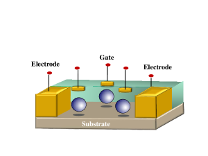
Fig.  1: Illustration of the TQDM junction system of interest.

We adopt the equation of motion method (EOM), which is a powerful tool for studying electron transport, taking into account electron Coulomb interactions.^{15, 16, 17, 18} This method has been applied to reveal the transport behaviors of a single QD with multiple energy levels¹⁶ and DQDs.^{17, 18} For a TQDM with one level per QD, there are 64 configurations for electrons to transport between electrodes.²⁰ Previous theoretical works have ignored the high-order Green functions resulting from electron Coulomb interactions to simplify the calculation.²⁰ To have a full solution becomes crucial for depicting the charge transport involving a few electrons. We solve the EOM of Green functions up to six electrons, taking into account all correlations caused by electron Coulomb interactions and electron hopping between TQDM. This involves solving 4752 Green’s functions and 923 correlation functions self-consistently.

2 Model

We consider an artificial molecule made of nanoscale QDs, in which the energy level separations are much larger than the on-site Coulomb interactions and thermal energies. Thus, only one energy level for each quantum dot is included. The extended Hubbard-Anderson model is employed to simulate the TQDM junction with Hamiltonian given by $H=H_{0}+H_{T}+H_{QDs}$, where $H_{0}=\sum_{{\bf k},\sigma,\alpha}\epsilon_{{\bf k}}c^{\dagger}_{{\bf k},\sigma,\alpha}c_{{\bf k},\sigma,\alpha}$ is the Hamiltonian for free electrons in the electrodes. $c^{\dagger}_{k,\sigma,\alpha}$($c_{{\bf k},\sigma,\alpha}$) creates (destroys) an electron of momentum k and spin $\sigma$ with energy $\epsilon_{k}$ in the $\alpha$ electrode. $H_{T}=\sum_{{\bf k},\ell,\alpha}(V_{k,\alpha,\ell}c^{\dagger}_{{\bf k},\sigma,\alpha}d_{\ell,\sigma}+V^{*}_{{\bf k},\alpha,\ell}d^{\dagger}_{\ell,\sigma}c_{{\bf k},\sigma,\alpha})$. $V_{{\bf k},\alpha,\ell}$ describes the coupling between the $\alpha$ electrode and the $\ell$-th QD. $d^{\dagger}_{\ell,\sigma}$ ($d_{\ell,\sigma}$) creates (destroys) an electron in the $\ell$-th dot. $H_{QDs}$ is the extended Hubbard Hamiltonian for multiple QDs.

$$H_{QDs} = \sum_{\ell,\sigma}E_{\ell}n_{\ell,\sigma}+\sum_{\ell}U_{\ell}n_{\ell,\sigma}n_{\ell,\bar{\sigma}}$$

$$+\sum_{\ell<j,\sigma,\sigma^{\prime}}U_{\ell j}n_{\ell,\sigma}n_{j,\sigma^{\prime}}+\sum_{\ell\neq j,\sigma}t_{\ell j}d^{\dagger}_{\ell,\sigma}d_{j,\sigma},$$

where $E_{\ell}$ is the spin-independent QD energy level, $n_{\ell,\sigma}=d^{\dagger}_{\ell,\sigma}d_{\ell,\sigma}$, $U_{\ell}$ and $U_{\ell j}$ ($\ell<j$) denote the intradot and interdot Coulomb interactions, respectively and $t_{\ell j}$ describes the electron interdot coupling. The interdot Coulomb interactions as well as intradot Coulomb interactions are important for nanoscale semiconductor QDs and molecules. Therefore, $U_{\ell,j}$ cannot be ignored.

Using the Keldysh-Green’s function technique^{15, 21}, the electrical current from reservoir $\alpha$ to the TQDM junction is calculated according to the Meir-Wingreen formula

$$J_{\alpha}=\frac{ie}{h}\int{d\epsilon}\sum_{j\sigma}\Gamma^{\alpha}_{j}[G^{<}_{j\sigma}(\epsilon)+f_{\alpha}(\epsilon)(G^{r}_{j\sigma}(\epsilon)-G^{a}_{j\sigma}(\epsilon))],$$ (2)

where $\Gamma^{\alpha}_{j}(\epsilon)=\sum_{\bf k}|V_{{\bf k},\alpha,j}|^{2}\delta(\epsilon-\epsilon_{\bf k})$ is the tunneling rate between the $\alpha$-th reservoir and the $j$-th QD. Throughout the paper, for two-terminal devices we assume that the left (right) lead is only coupled to the left (right) QD with tunneling rate $\Gamma_{L}$ ($\Gamma_{R}$), while there is no coupling between the center QD and the two leads. For three-terminal devices, the coupling between the center QD and a third gate is described by the tunneling rate $\Gamma_{C}$. $f_{\alpha}(\epsilon)=1/\{\exp[(\epsilon-\mu_{\alpha})/k_{B}T]+1\}$ denotes the Fermi distribution function for the $\alpha$-th electrode, where $\mu_{\alpha}$ is the chemical potential and $T$ is the temperature of the system. $e$, $h$, and $k_{B}$ denote the electron charge, the Planck’s constant, and the Boltzmann constant, respectively. $G^{<}_{j\sigma}(\epsilon)$, $G^{r}_{j\sigma}(\epsilon)$, and $G^{a}_{j\sigma}(\epsilon)$ are the frequency domain representations of the one-particle lessor, retarded, and advanced Green’s functions $G^{<}_{j\sigma}(t,t^{\prime})=i\langle d_{j,\sigma}^{\dagger}(t^{\prime})d_{j,\sigma}(t)\rangle$, $G^{r}_{j\sigma}(t,t^{\prime})=-i\theta(t-t^{\prime})\langle\{d_{j,\sigma}(t),d_{j,\sigma}^{\dagger}(t^{\prime})\}\rangle$, and $G^{a}_{j\sigma}(t,t^{\prime})=i\theta(t^{\prime}-t)\langle\{d_{j,\sigma}(t),d_{j,\sigma}^{\dagger}(t^{\prime})\}\rangle$, respectively. These one-particle Green’s functions are related recursively to other Green’s functions and correlators via the many-body equation of motion,^{16, 17, 18} which we solve via an iterative numerical procedure to obtain all $n$-particle Green’s functions ($n=1,\cdots,6$) and correlators for the TQDM. (See supplemental materials.) Our procedure is valid in the Coulomb blockade regime, but not the Kondo regime.^{22, 23} Throughout this paper, we assume the on-site Coulomb interaction $U_{\ell}=U_{0}=100\Gamma_{0}$ for all three QDs and the same tunneling rates at all leads, $\Gamma^{\alpha}_{j}=\Gamma$ with $j$ labeling the QD directly connected to lead $\alpha$.

3 Results and discussion

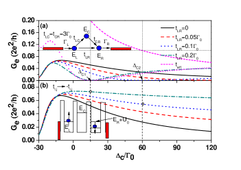
Fig.  2: Electrical conductance ($G_{e}$) of TQDM as a function of central QD energy for different $t_{LR}$ strengths in the Pauli spin blockade configuration with $E_{L}=E_{F}$ and $E_{R}=E_{F}-U_{R}$. (a) $t_{LC}=t_{CR}=3\Gamma_{0}$, and (b) $t_{\ell,j}$ replaced by $-t_{\ell,j}$. Other physical parameters are $k_{B}T=1\Gamma_{0}$, $\Gamma=0.3\Gamma_{0}$, $U_{LC}=U_{CR}=30\Gamma_{0}$, and $U_{LR}=0$.

Although the QI of TQDM was theoretically investigated previously^{24, 25}, the effect of intradot and interdot Coulomb interactions was not considered. Here, we utilize the LDCT effect to tune the effective hopping strength between outer QDs to achieve the destructive and constructive QIs in the presence of electron Coulomb interaction. We consider a TQDM junction in the Pauli spin blockade (PSB) configuration^{4, 18} with $E_{L}=E_{F}$, $E_{R}=E_{F}-U_{0}$, $t_{LC}=t_{CR}=3\Gamma_{0}$, $\Gamma_{L}=\Gamma_{R}=0.3\Gamma_{0}$, $U_{LC}=U_{CR}=30\Gamma_{0}$, and $U_{LR}=0$. Fig. 2(a) shows the electrical conductance ($G_{e}$) as a function of central QD energy level ($\Delta_{C}=E_{C}-E_{F}$) for $t_{LR}$ varying from 0 to $0.2\Gamma_{0}$ at $k_{B}T=1\Gamma_{0}$ (in weak interdot coupling regime). For $\Delta_{C}$ less than $-15\Gamma_{0}$, $G_{e}$ is not sensitive to the variation of $t_{LR}$, indicating that the transport is mainly through the upper path involving the center QD as shown in the inset of Fig. 2(a). In the case of $t_{LR}=0$, $G_{e}$ can be well explained by the LDCT effect when $E_{C}$ is far away from $E_{F}$.²⁶ The central QD provides an intermediated state for electrons in the outer QDs. Through the upper path, TQDM behaves like a double QD with an effective hopping $t_{eff}=-t_{LC}t_{CR}/(U_{CR}+\Delta_{C})$, which can also be understood by the second order perturbation theory.²⁶ Once $t_{LR}\neq 0$ (the lower path turns on), electron transport through the two paths with $t_{eff}$ and $t_{LR}$ lead to a destructive QI. Note that $G_{e}$ for the case of $t_{LR}\neq 0$ is reduced compared to the case of $t_{LR}=0$. In particular, $G_{e}$ is vanishingly small at the value of $\Delta_{C}$ where $|t_{eff}|$ crosses $t_{LR}$ as indicated by dashed lines in Fig. 2(a). For illustration, the curve for $|t_{eff}|=|t_{LC}t_{CR}|/(U_{CR}+\Delta_{C})$ is also shown in Fig. 2(a). (See short-dashed curve) The vanishing $G_{e}$ occurs at lower $\Delta_{C}$ with increasing $|t_{LR}|$ (Compare dash-dotted with dashed curves). Due to topological effect, the electron-hole symmetry does not hold for the energy spectrum of TQDM.¹³ When TQDM has identical QD energy levels ($E_{\ell}=E_{0}$) and homogenous electron hopping strengths $t_{\ell,j}=t$, we have one level $\epsilon=E_{0}+2t$ and one doubly degenerate level with $\epsilon=E_{0}-t$ for the case of $U_{\ell}=U_{\ell,j}=0$. Unlike the cases of DQDs and SCTQDs, the lowest energy level depends on the sign of $t_{\ell,j}$. This is a manifesting result of electron-hole asymmetrical behavior of TQDM. Therefore, it will be interesting to examine the sign effect of $t_{\ell,j}$ on the QI behavior. Physically, the sign of $t_{\ell,j}$ depends on the symmetry properties of orbitals, which can change in different configurations. We can replace $t_{\ell,j}$ by $-t_{\ell,j}$ to examine the QI effect with respect to the electron-hole symmetry. The results are shown in Fig. 2(b). We find that $G_{e}$ is enhanced with increasing $t_{LR}$, which is attributed to the constructive QI effect, in contrast to the destructive QI effect shown in Fig. 2(a).

To gain deeper understanding of the destructive and constructive QI shown in Fig. 2, we compare our full calculation with the weak interdot-coupling theory,^{18, 26} which allows simple closed-form expression for the electrical conductance of TQDM. We obtain $G_{e}=2e^{2}/h\int d\epsilon{\cal T}(\epsilon)[\partial f(\epsilon)/\partial E_{F}]\approx(2e^{2}/h){\cal T}(E_{F})$ at low-temperature limit, where the transmission coefficient ${\cal T}(\epsilon)$ with 64 configurations is approximately given by

$${\cal T}_{PSB}(\epsilon)$$ (3)

$$=\frac{4\Gamma_{L}\Gamma_{R}P_{PSB}F_{QI}}{|\mu_{1}\mu_{2}\mu_{3}-t^{2}_{CR}\mu_{1}-t^{2}_{LC}\mu_{3}-t^{2}_{LR}\mu_{2}-2t_{LR}t_{LC}t_{CR}|^{2}},$$

where $F_{QI}=\mu^{2}_{2}(t_{LC}t_{CR}/\mu_{2}+t_{LR})^{2}$ is a factor related to QI. $\mu_{1}=\epsilon-E_{L}+i\Gamma_{L}$, $\mu_{2}=\epsilon-E_{C}-U_{RC}$ and $\mu_{3}=\epsilon-E_{R}-U_{R}+i\Gamma_{R}$. $P_{PSB}$ denotes the probability weight in the PSB configuration.¹⁸ From Eq. (3), we have

$$G_{e}=\frac{2e^{2}}{h}\frac{P_{PSB}4\Gamma^{2}(t_{eff}+t_{LR})^{2}}{(\Gamma^{2}+2t_{eff}t_{LR}+t^{2}_{LR})^{2}+\Gamma^{2}~{}(t_{h1}+t_{h2})^{2}},$$ (4)

where $t_{eff}=-t_{LC}t_{CR}/(U_{CR}+\Delta_{C})$, $t_{h1}=-t^{2}_{LC}/(U_{CR}+\Delta_{C})$, and $t_{h2}=-t^{2}_{CR}/(U_{CR}+\Delta_{C})$ with $\Gamma_{L}=\Gamma_{R}\equiv\Gamma$. For $t_{LC}=t_{CR}=t_{c}=0$, Eq. (4) reduces to the conductance of DQD,¹⁷ while for $t_{LR}=0$, it reduces to the $G_{e}$ of SCTQD.²⁶ At $\Delta_{C}=15\Gamma_{0}$ and $60\Gamma_{0}$, which satisfy the condition of $t_{eff}+t_{LR}=0$ for $t_{LR}=0.2\Gamma_{0}$ and $t_{LR}=0.1\Gamma_{0}$, respectively, and we see $G_{e}$ vanishes there. This well illustrates the destructive QI seen in Fig. 2(a). Once we make the substitution $t_{\ell,j}\rightarrow-t_{\ell,j}$ in Eq. (4), we can reveal the constructive QI in $G_{e}$ as shown in Fig. 2(b). Note that in the weak coupling regime ($t_{eff}/\Gamma\ll 1$), the probability weight $P_{PSB}$ of Eq. (4) calculated according to the procedures in Ref. 18, where the interdot two-particle correlation functions are factorized as the product of single occupation numbers, is consistent with the full calculation, but not for $t_{eff}/\Gamma\gg 1$. Away from the weak coupling regime, the interdot electron correlations become important. To explicitly reveal the importance of electron correlation effects, we plot the curve of $t_{LR}=0.2\Gamma_{0}$ (with triangle marks) calculated by the procedure of Ref. 18 (including 64 configurations) in Fig. 2(a). Comparison between the full solution and the approximation considered in Ref. 18, we find that the electron correlation effects become very crucial when $t_{eff}/\Gamma\gg 1$. Once electron transport involves more electrons, the high-order (beyond two-particle) Green functions and correlation functions should be included (see the results of Fig. 3). The difference between the conventional mean-field theory of Ref. 3 with the full solution is even larger. The comparison between mean-field theory and the procedure of Ref. 18 has been discussed in the appendix of Ref. 18.

According to Eq. (4), constructive and destructive QI effects depend on the sign of $t_{\ell,j}$. Therefore, if the wavefunction of the center dot has opposite parity (say, an $x$-like state) with respect to the wavefunctions in two outer dots (assumed to be $s$-like), then $t_{LC}$ will have opposite sign compared with $t_{CR}$ and $t_{LR}$, and the sign of $t_{eff}$ will be flipped. Consequently, the destructive QI shown in Fig. 2(a) will become constructive QI. Thus, for a center QD with an $s$-like ground state and an excited $p$-like state, it is possible to see the change of QI between destructive and constructive by tuning the gate voltage, which sweeps through different resonance energies of the center QD in addition to the change of sign of $t_{eff}$ when the Fermi level goes from below the resonance level to above the resonance level. From the results of Fig. 2, QI effect can be electrically controlled by the energy level $E_{c}$. This advantage of TQDM may be useful for improving the spin filtering of DQDs ⁴.

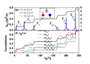
Fig.  3: (a) Electrical conductance of TQDMs as a function of gate voltage $\Delta_{g}$ with $E_{L}=E_{R}=E_{C}=E_{F}+10\Gamma_{0}-\Delta_{g}$ and $\Gamma=1.6\Gamma_{0}$.(b) Correlation functions for $k_{B}T=0\Gamma_{0}$. Other physical parameters are $t_{\ell,j}=3\Gamma_{0}$ and $U_{LR}=U_{LC}=U_{CR}=30\Gamma_{0}$.

In addition to QI effects, spin frustration and topological effects (due to electron-hole asymmetry) on the measured quantities (electrical conductance or current) are also interesting issues.¹¹ Fig. 3(a) shows $G_{e}$ as a function of gate voltage, $\Delta_{g}$ for $E_{\ell}=E_{F}+10\Gamma_{0}-\Delta_{g}$; $\ell=L,C,R$ at two different temperatures, $k_{B}T=0$ and $1\Gamma_{0}$. Here, we consider the homogenous configuration with $U_{LR}=U_{LC}=U_{CR}=30\Gamma_{0}$ and $t_{\ell,j}=t_{c}=3\Gamma_{0}$. At low temperature, there are six main peaks in the $G_{e}$ spectrum, labeled by $\epsilon_{n}$, $n=1,\cdots,6$ and some secondary peaks. At higher temperature, the six main peaks are suppressed and broadened as shown by the dashed curve, and the secondary peaks are washed out. We also plot the total occupation number, $N=\sum_{\sigma}(N_{L,\sigma}+N_{R,\sigma}+N_{C,\sigma})$ as the black solid curve, which shows a stair-case behavior with plateaus at $N=1,\cdots,6$, corresponding to the filling of TQDM with 1 to 6 electrons. It can be seen that the six main peaks occur at $\Delta_{g}$ where $N$ is increased by 1. Thus, the peak positions $\epsilon_{n}$ correspond to the chemical potential of electrons in TQDM, i.e. the energy needed to add an electron to the system. The main peak positions can be approximately obtained by the calculation of chemical potential of TQDM without considering the coupling with leads as done in Ref. 13. For example, $\epsilon_{1}=E_{L}-2|t_{c}|$, $\epsilon_{2}=E_{L}+U_{LC}-8t^{2}/(U_{0}-U_{LC})$ and $\epsilon_{3}=E_{L}+2U_{\ell,j}-3J_{ex}/2+2|t_{c}|+16t^{2}_{c}/(U_{0}-U_{LC})$ under the condition $U_{0}>U_{LC}\gg t_{c}$, where $J_{ex}\equiv E_{0}(S=3/2)-E_{0}(S=1/2)$ is the difference in energy between the spin-3/2 and spin-1/2 configuration.¹³ However, the relative strengths of peaks in the conductance spectrum can only be obtained by solving the full Anderson-Hubbard model self-consistently.

Unlike the $G_{e}$ spectrum of DQDs,¹⁷ the $G_{e}$ spectrum of TQDM does not show the electron-hole symmetry due to topological effect. Note that $N=4$ and $N=5$ correspond to two-hole and one-hole configurations, respectively. A large Coulomb blockade separation between $\epsilon_{3}$ and $\epsilon_{4}$ is given by $\Delta_{34}=U_{0}+3J_{ex}-4t_{c}-8t^{2}_{c}/(U_{0}-U_{LC})$. Here, $\epsilon_{4}$ corresponds to the two hole ground state with spin triplet instead of singlet. The magnitude of $G_{e}$ is smaller than the quantum conductance $2e^{2}/h$ for $t_{LR}/\Gamma\gg 1$ as a result of electron Coulomb interactions.¹⁷ The mechanism for understanding the unusual $G_{e}$ behavior in nanostructure junction systems is a subject of high interest.²⁷ Due to electron Coulomb interactions, the magnitudes of peaks are related to the probability weights of quantum paths, which are related to single-particle occupation numbers and many-particle correlation functions.¹⁸

To reveal the configurations for each main peak, the one-particle occupation number $N_{\ell,\sigma}\equiv\langle n_{\ell,\sigma}\rangle$, interdot two particle correlation functions $\langle n_{\ell,\sigma}n_{j,\bar{\sigma}}\rangle$ , and three particle correlation functions ($\langle n_{L,\sigma}n_{C,-\sigma}n_{R,\sigma}\rangle$, and $\langle n_{L,\sigma}n_{C,-\sigma}n_{R,\sigma}\rangle$) are plotted in Fig. 3(b). We always have the relation $N_{L,\sigma}=N_{R,\sigma}\neq~{}N_{C,\sigma}$, because the outer QDs are directly coupled to electrodes, but not the central QD. Such a relation also holds for two-particle and three-particle correlation functions. The six main peaks in Fig. 3(a) indicate the filling of TQDM up to the $n$-electron ground state for $n=1,\cdots,6$. For example, $\epsilon_{2}$ indicates the formation of two-electron state with spin singlet, while $\epsilon_{3}$ indicates the formation of three-particle state with total spin $S=1/2$, which can be described as the spin-frustration state^{11, 13, 28}. Because the on-site Coulomb interaction favors homogeneous distribution of three electrons in TQDM, whereas the interdot Coulomb repulsion favors the charge fluctuation. As seen in Fig. 3(b), for $\Delta_{g}\leq\epsilon_{3}$ ($~{}78\Gamma_{0}$) $N_{\ell}$ in each dot clearly displays the charge fluctuation behavior. When TQDM goes into a three-particle state ($\Delta_{g}>\epsilon_{3}$), the charge fluctuation is suppressed, and each QD is filled with one particle (with $N_{L,\sigma}=N_{R,\sigma}=N_{C,\sigma}=0.5$), while $\langle n_{L,\sigma}n_{C,\sigma}n_{R,-\sigma}\rangle$=$\langle n_{L,\sigma}n_{C,-\sigma}n_{R,\sigma}\rangle=\langle n_{L,-\sigma}n_{C,\sigma}n_{R,-\sigma}\rangle$. This also demonstrates the spin frustration condition as depicted in the inset of Fig. 3(a).

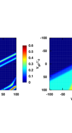
Fig.  4: Charge stability diagram of TQDM. $\Gamma_{\ell}=\Gamma_{0}$, $k_{B}T=1.5\Gamma_{0}$, $U_{LC}=U_{CR}=U_{LR}=12\Gamma_{0}$, $t_{\ell,j}=3\Gamma_{0}$. The energy levels are shifted according to $E_{\ell}=E_{F}-U_{LR}-\sum_{m=1}^{2}\beta_{\ell,m}eV_{gm}$, where the gate coupling constants are $\beta_{L,1}=0.5$, $\beta_{C,1}=1$, $\beta_{R,1}=0.5$, $\beta_{L,2}=1$, $\beta_{C,2}=0.5$, and $\beta_{R,2}=1$.

Figure 4 shows the charge stability diagram for zero-bias electrical conductance ($G_{e}$) and total occupation number ($N$) as functions of gate voltages exerted on any two QDs (labeled by $V_{g1}$ and $V_{g2}$) for a TQDM connected to three terminals. The magnitudes of $G_{e}$ and $N$ are indicated by different colors. It is noticed that $G_{e}$ is enhanced on the borders that separate domains of different values of occupation number ($N$) with larger $G_{e}$ occurring at $V_{g1}=V_{g2}$. This is a result of higher degeneracy and charge-fluctuation in the state. The largest $G_{e}$ for $N\leq 3$ occurs at the junction between $N=1$ and $N=2$ domains when $V_{g1}=V_{g2}$. This feature corresponds to the $\epsilon_{2}$ peak of Fig. 3(a). The diagram Fig. 4(a) is simply a collection of curves displayed in Fig. 3(a) at different values of $V_{g2}$ that shifts the QD energy levels. We note that in the domains of $N=1$ and $N=2$, the areas with stripes are not symmetrical with respect to gate voltage. In Ref. 11, a capacitive interaction model was employed to plot the diagram of $N$. In their model, the electron hopping strength $t_{\ell,j}$ was ignored. Consequently, the charge stability diagram of $G_{e}$ cannot be obtained. The charge stability diagram of $G_{e}$ obtained by our full calculation [as shown in Fig. 4(a)] bears close resemblance to the experimental results as shown in Fig. 2 of Ref. 11.

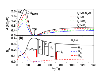
Fig.  5: (a) Tunneling current as a function of $\Delta_{C}=E_{C}-E_{F}$ at finite bias $V_{a}=10\Gamma_{0}$ for various temperatures. (b) Occupation numbers as a function of $\Delta_{C}$ at $k_{B}T=0$. The other physical parameters used are $E_{L}=E_{R}=E_{F}+10\Gamma_{0}$, $U_{LC}=U_{CR}=30\Gamma_{0}$, $U_{LR}=10\Gamma_{0}$, $t_{LC}=t_{CR}=3\Gamma_{0}$, $t_{LR}=0.4\Gamma_{0}$, and $\Gamma=\Gamma_{0}$.

So far, the results shown in Figs. 2-4 are all related to the linear response. To further clarify the QI effect at finite bias ($V_{a}=10\Gamma_{0}$) for different temperatures, we plot in Fig. 5(a) the tunneling current as a function of center QD energy, $E_{C}=E_{F}+\Delta_{c}$ for the configuration shown in the inset of Fig. 5(b). For $\Delta_{C}\geq 2\Gamma_{0}$, the tunneling current is suppressed as temperature increases. This is attributed to a reduction of electron population in the electrodes for electrons with energy near $E_{F}+10\Gamma_{0}$. For $\Delta_{C}\leq 2\Gamma_{0}$, we notice that $N_{c,\sigma}$ quickly jumps to 0.4, indicating that the central QD is filled with charge, which causes an interdot Coulomb blockade for electrons entering the left QD. (See the reduction of $N_{L,\sigma}$ in Fig. 5(b)). This explains the sharp dip of $G_{e}$ for $\Delta_{C}\leq 2\Gamma_{0}$ in Fig. 5(a). As temperature increases, such a dip in tunneling current is smeared out. At $\Delta_{C}=10\Gamma_{0}+t_{LC}t_{CR}/t_{LR}\equiv\Delta_{QI}$, the tunneling current vanishes for all temperatures considered due to the QI effect. Such a robust destructive QI effect with respect to temperature provides a remarkable advantage for the realization of single electron QI transistors at room temperature.¹² To understand the interdot correlation effect, we also plot the case without interdot Coulomb interaction ($U_{\ell,j}=0$) for $k_{B}T=0$ in Fig. 5(a). (See solid curve) We notice that the QI effect remains qualitatively the same, except that the tunneling current is slightly enhanced with interdot Coulomb interaction turned off. As the QI effect suppresses the current flow, the charge will accumulate in the left dot. Thus, $N_{L,\sigma}$ reaches the maximum at $\Delta_{C}=\Delta_{QI}$ while $N_{R}$ reaches the minimum as seen in Fig. 5(b). This implies that the QI effect can be utilized to control charge storage in TQDM.

4 Conclusions

In summary we have obtained full solution to the charge transport through TQDM junction in the presence of electron Coulomb interactions, which includes all $n$-electron ($n=1,\cdots,6$) Green’s functions and correlation functions. The destructive and constructive QI behaviors of TQDM are clarified by considering the LDCT effect on the conductance spectrum. The conductance spectrum of TQDM with total occupation number varying from one to six directly reveals the electron-hole asymmetry due to topological effect. The calculated correlation functions also illustrate the charge fluctuation and spin frustration behaviors of TQDM. Our numerical results for charge stability diagram match experimental measurements very well. Finally, we demonstrated that the QI effect in TQDM is robust against temperature variation and it can be utilized to control the charge storage.

Acknowledgments
This work was supported in part by the National Science Council, Taiwan under Contract Nos. NSC 101-2112-M-001-024-MY3 and NSC 103-2112-M-008-009-MY3.

References

- Reed et al. 1997 M. A. Reed, C. Zhou, C. J. Muller, T. P. Burgin and J. M. Tour, Science, 1997, 278, 252–254.
- Joachim et al. 2000 C. Joachim, J. Gimzewski and A. Aviram, Nature, 2000, 408, 541–548.
- Bergfield and Stafford 2009 J. Bergfield and C. Stafford, Phys. Rev. B, 2009, 79, 245125.
- Hanson et al. 2007 R. Hanson, L. P. Kouwenhoven, J. R. Petta, S. Tarucha and L. M. K. Vandersypen, Rev. Mod. Phys., 2007, 79, 1217–1265.
- Busl et al. 2013 M. Busl, G. Granger, L. Gaudreau, R. Sánchez, A. Kam, M. Pioro-Ladrière, S. A. Studenikin, P. Zawadzki, Z. R. Wasilewski, A. S. Sachrajda and G. Platero, Nature nanotechnology, 2013, 8, 261–265.
- Braakman et al. 2013 F. R. Braakman, P. Barthelemy, C. Reichl, W. Wegscheider and L. M. K. Vandersypen, Nature nanotechnology, 2013, 8, 432–437.
- Amaha et al. 2013 S. Amaha, W. Izumida, T. Hatano, S. Teraoka, S. Tarucha, J. A. Gupta and D. G. Austing, Phys. Rev. Lett., 2013, 110, 016803.
- Nitzan and Ratner 2003 A. Nitzan and M. A. Ratner, Science, 2003, 300, 1384–1389.
- Stafford et al. 2007 C. A. Stafford, D. M. Cardamone and S. Mazumdar, Nanotechnology, 2007, 18, 424014.
- Pöltl et al. 2013 C. Pöltl, C. Emary and T. Brandes, Phys. Rev. B, 2013, 87, 045416.
- Seo et al. 2013 M. Seo, H. K. Choi, S.-Y. Lee, N. Kim, Y. Chung, H.-S. Sim, V. Umansky and D. Mahalu, Phys. Rev. Lett., 2013, 110, 046803.
- Guédon et al. 2012 C. M. Guédon, H. Valkenier, T. Markussen, K. S. Thygesen, J. C. Hummelen and S. J. van der Molen, Nature nanotechnology, 2012, 7, 304–309.
- Korkusinski et al. 2007 M. Korkusinski, I. P. Gimenez, P. Hawrylak, L. Gaudreau, S. A. Studenikin and A. S. Sachrajda, Phys. Rev. B, 2007, 75, 115301.
- Hsieh et al. 2012 C.-Y. Hsieh, Y.-P. Shim and P. Hawrylak, Phys. Rev. B, 2012, 85, 085309.
- Meir and Wingreen 1992 Y. Meir and N. S. Wingreen, Phys. Rev. Lett., 1992, 68, 2512–2515.
- Kuo and Chang 2007 D. M.-T. Kuo and Y.-C. Chang, Phys. Rev. Lett., 2007, 99, 086803.
- Bułka and Kostyrko 2004 B. R. Bułka and T. Kostyrko, Phys. Rev. B, 2004, 70, 205333.
- Kuo et al. 2011 D. M.-T. Kuo, S.-Y. Shiau and Y.-C. Chang, Phys. Rev. B, 2011, 84, 245303.
- Loss and DiVincenzo 1998 D. Loss and D. P. DiVincenzo, Phys. Rev. A, 1998, 57, 120–126.
- Weymann et al. 2011 I. Weymann, B. Bułka and J. Barnaś, Phys. Rev. B, 2011, 83, 195302.
- Haug and Jauho 2007 H. Haug and A.-P. Jauho, Quantum kinetics in transport and optics of semiconductors, Springer, 2007.
- Goldhaber-Gordon et al. 1998 D. Goldhaber-Gordon, H. Shtrikman, D. Mahalu, D. Abusch-Magder, U. Meirav and M. A. Kastner, Nature, 1998, 391, 156–159.
- Numata et al. 2009 T. Numata, Y. Nisikawa, A. Oguri and A. C. Hewson, Phys. Rev. B, 2009, 80, 155330.
- Michaelis et al. 2006 B. Michaelis, C. Emary and C. Beenakker, EPL (Europhysics Letters), 2006, 73, 677.
- Emary 2007 C. Emary, Phys. Rev. B, 2007, 76, 245319.
- Kuo and Chang 2014 D. M. T. Kuo and Y.-C. Chang, Phys. Rev. B, 2014, 89, 115416.
- Bauer et al. 2013 F. Bauer, J. Heyder, E. Schubert, D. Borowsky, D. Taubert, B. Bruognolo, D. Schuh, W. Wegscheider, J. von Delft and S. Ludwig, Nature, 2013, 501, 73–78.
- Andergassen 2013 S. Andergassen, Nature, 2013, 495, 321–322.