Ising interaction between capacitively-coupled superconducting flux qubits

Abstract

Here, we propose a scheme to generate a controllable Ising interaction between superconducting flux qubits. Existing schemes rely on inducting couplings to realize Ising interactions between flux qubits, and the interaction strength is controlled by an applied magnetic field On the other hand, we have found a way to generate an interaction between the flux qubits via capacitive couplings. This has an advantage in individual addressability, because we can control the interaction strength by changing an applied voltage that can be easily localized. This is a crucial step toward the realizing superconducting flux qubit quantum computation.

I Introduction

To realize fault-tolerant quantum computation, it is crucial to investigate a scheme to generate a cluster state in a scalable way. The cluster state is a universal resource for quantum computation, and this state can be used for a fault-tolerant scheme such as a surface code and topological code. One can generate a cluster state if we can turn on/off an Ising type interaction between qubits.

Superconducting circuit is one of the promising systems to realize such a cluster-state quantum computation. Josephson junctions in the superconducting circuit can induce a non-linearity, and so one can construct a two-level system. There are several types of Josephson junction qubit: charge qubit Chen et al. (2007), superconducting spin qubit Padurariu and Nazarov (2010), superconducting flux qubit Billangeon et al. ; Chiorescu et al. (2003); Niskanen et al. (2006); Bylander et al. (2011a); Yoshihara et al. (2014), superconducting phase qubit Ansmann et al. (2009); Hofheinz et al. (2009); Steffen et al. (2006), superconducting transmon qubit DiCarlo et al. (2009); Koch et al. (2007), fluxonium qubit Manucharyan et al. (2009); Zhu et al. (2013), and several hybrid systems You et al. (2007); Steffen et al. (2010).

The transmon qubit DiCarlo et al. (2009); Koch et al. (2007); Barends et al. (2013), which is a cooper-pair box and relatively insensitive to low-frequency charge noise, is considered one of the powerful method of the qubit implementation by using superconducting circuit. Scheme of the tunable qubit-qubit capacitive coupling is proposed and demonstrated Ghosh et al. (2013); Chen et al. (2014); Geller et al. (2014). The high fidelity qubit readout using a microwave amplifier is demonstrated Sete et al. (2013); Hover et al. (2014); Jeffrey et al. (2014). Furthermore, high fidelity (99.4%) two-qubit gate using five qubits system is achieved. This result is the first step toward surface code scheme Barends et al. (2014). These results show a good scalability towards the realization of generating a large scale cluster state.

The flux qubit consist of a superconducting loop containing several Josephson junctions. This system has a large anharmonicity and can be well approximated to a two-level system. Single qubit gate operations can be realized with high speed and reasonable fidelity Yoshihara et al. (2014). Meanwhile, the best observed coherence time is an order of $10$ $\mu s$ Bylander et al. (2011b); Stern et al. (2014). Furthermore, the tunable coupling schemes for two qubit gate operations are proposed and demonstrated Plourde et al. (2004); Grajcar et al. (2006); Hime et al. (2006); van der Ploeg et al. (2007); Niskanen et al. (2007); Harris et al. (2007); Ashhab et al. (2008); Yamamoto et al. (2008); Groszkowski et al. (2011). Quantum non-demolition measurement of flux qubit during the coherence time is realized by using Josephson bifurcation amplifier Siddiqi et al. (2006, 2004); Jordan and Smith (2007); Kakuyanagi et al. (2013).

There are two typical tunable qubit-qubit coupling schemes, inductive coupling and capacitive coupling. In flux qubit system, existing schemes rely on inductive coupling with the external magnetic field. Several schemes of the tunable qubit-qubit inductive coupling are proposed and demonstrated Plourde et al. (2004); Grajcar et al. (2006); Hime et al. (2006); van der Ploeg et al. (2007); Niskanen et al. (2007); Harris et al. (2007); Ashhab et al. (2008); Yamamoto et al. (2008); Groszkowski et al. (2011). However, it is hard to apply magnetic field to a localized region. Due to this property, it is difficult to achieve individual addressability of all qubits, because magnetic field may affect not only the target qubits but also other qubits as well. Therefore, it is important to perform two-qubit gates without affecting other qubits by using localized fields for scalable quantum computation.

Here, we propose a way to generate and control the Ising type interaction between four-junction flux qubits using capacitive coupling. By using an applied voltage, we control the interaction between flux qubits that are connected by capacitance. Unlike the standard schemes, our scheme does not require to change the applied magnetic field on the flux qubit for the control of the interaction. This may have advantage to implement two-qubit gates on the target qubits without affecting other qubits because applying local voltages is typically much easier than applying local magnetic flux. We take into account of realistic noise on this type of flux qubits, and estimate a qubit-parameter range where one can perform fault-tolerant quantum computation. Furthermore, we show a way to generate a two dimensional cluster state in a scalable way. Our result paves the way to achieve the scalable quantum computation with superconducting flux qubits.

The rest of this paper is organized as follows: In Section , we presents the design details of our flux qubit and effects on a flux qubit from the change of the parameters. In Section III, we propose our scheme for generating Ising type interaction between capacitively coupled superconducting flux qubits. Moreover, we show the relationship between coupling strength and two types of errors caused by operation accuracy, the fluctuation of applied voltage and timing jitter. In Section IV, we present the analysis of our scheme for use in multi-qubit system. Additionally, we discuss how to suppress the non-nearest neighbor interactions by changing parameters and performing $\pi$ pulses. Furthermore, we show our procedure for generating a one and two-dimensional cluster state using qubits on square lattice in less time.

II Voltage controlled $\alpha$-tunable flux qubit

Let us first show the circuit of a flux qubit that we propose in Fig. 1.

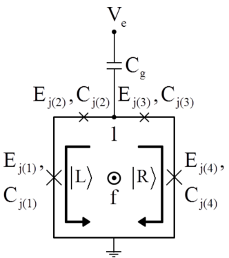
Figure 1: (a)The circuit of a flux qubit in our design. This flux qubit has four Josephson junctions (JJ). $E_{j(n)}$ and $C_{j(n)}$ denote the Josephson energy and capacitance of $n$ th Josephson junction JJ$n$. The loop is threaded by an external magnetic flux $f$, and we can control the energy bias of the qubit via the magnetic flux. Node $1$ represents the superconducting island. The electric potential of node $1$ is $V_{i}$. (b) The $\alpha$ dependence of $E_{01}$ and $E_{12}$ where $E_{01}$ denotes energy difference between the ground state and the first excited state, $E_{12}$ denotes energy difference between the first excited state and the second excited state. Here, we set $E_{j(1)}=E_{j(4)}=200$ GHz, $E_{j(2)}=E_{j(3)}=40$ GHz, and $E_{j(k)}/E_{c(k)}=80(k=1,2,..,4)$.

Here, X-shaped crosses denote Josephson junctions (JJ). The first Josephson junctions (JJ$1$) and the fourth Josephson junctions (JJ$4$) both have the same Josephson energies $E_{j}$ and capacitances $C_{j}$. The second Josephson junctions (JJ$2$) and the third Josephson junction (JJ$3$) both have the same Josephson energies and capacitances that are $\alpha$ times larger than those of JJ$1$ and JJ$4$. Josephson phases $\varphi_{n}$, which is given by the gauge-invariant phase of each JJ$n$, are subject to the following equation:

$$\varphi_{1}+\varphi_{2}+\varphi_{3}+\varphi_{4}=-2\pi f$$ (1)

due to fluxoid quantization around the loop containing phases of Josephson junctions. $f$ denotes the external magnetic flux through the loop of the qubit in units of the magnetic flux quantum $\Phi_{0}=\frac{h}{2e}$. The total Josephson energy $U$ can be described as follows:

$${U} = \sum^{4}_{k=1}E_{j(k)}\left(1-\cos\varphi_{k}\right).$$ (2)

The total electric energy $T$ can be described as follows:

$$T = \frac{1}{2}\sum_{k=1}^{4}{C}_{j(k)}\left(\frac{\Phi_{0}}{2\pi}\dot{\varphi}_{k}\right)^{2}+\frac{1}{2}C_{g}\left(V_{e}-V_{i}\right)^{2}$$ (3)

where $C_{g}$, $V_{e}$ and $V_{i}$ denotes the capacitance of the gate capacitor, applied external voltage and the electric potential of node $1$, respectively. Here, node $1$ represents the superconducting island.

Although the system Hamiltonian $H$ has many energy levels, the system can be described as a two-level system (qubit) due to a strong anharmonicity by choosing suitable $\alpha$. We show the $\alpha$ dependence of the energy of this system Fig. 1, where $E_{01}$ ($E_{12}$) denotes the energy splitting between the ground (first excited) and the first excited (second excited) state. This clearly shows that system has an anharmonicity so that we can control only the ground state and first excited state by using frequency selectivity.

$\lvert g\rangle$ and $\lvert e\rangle$ are the ground and the first excited state of the system Hamiltonian $H=T+U$ for $f=0.5$. In this regime, the ground state and the first excited state of this system contains a superposition of clockwise and anticlockwise persistent currents. Here, $\lvert L\rangle=\frac{1}{\sqrt{2}}(\lvert g\rangle+\lvert e\rangle)$ corresponds anticlockwise persistent current and $\lvert R\rangle=\frac{1}{\sqrt{2}}(\lvert e\rangle-\lvert g\rangle)$ corresponds clockwise one.

While $f$ is around 0.5, due to the anharmonicity, we can consider only the ground state and first excited state in the Hamiltonian $H$, and so we can simplify the $H$ into $H_{ge}$ spanned by $\lvert g\rangle$ and $\lvert e\rangle$ as follows:

$$H_{ge} = \frac{1}{2}\left(\Delta\sigma_{Z}+\varepsilon\sigma_{Y}\right)$$ (4)

where $\sigma_{Z}=\lvert e\rangle\langle e\rvert-\lvert g\rangle\langle g\rvert$ and $\sigma_{Y}=-i\lvert e\rangle\langle g\rvert+i\lvert g\rangle\langle e\rvert$ are Pauli matrices, $\Delta$ denotes the tunneling energy between $\lvert L\rangle$ and $\lvert R\rangle$, $\varepsilon$ denotes the energy bias between $\lvert L\rangle$ and $\lvert R\rangle$. The energy of the qubit is described as $E_{01}=\sqrt{\varepsilon^{2}+\Delta^{2}}$.

In this paper, unless indicated otherwise, we fix parameters as $\alpha=0.2$ and $E_{j(1)}=200$ GHz and $E_{j(k)}/E_{c(k)}$ ratio is $80$. Here, $E_{c(k)}=e^{2}/2C_{j(k)}$ is charge energy of each Josephson junction. In this parameter regime, $E_{01}$ is about three times larger than $E_{12}$ as shown in Fig. 1 so that we could consider this system as an effective two-level system. When $f$ is set to be near $0.5$, the derivative of the qubit energy against the magnetic flux $\lvert\frac{dE_{01}}{df}\rvert$ takes the minimum value, so that the qubit should be well decoupled from flux noise, and we achieve the maximum coherent times. We call this regime “optimal point”. On the other hand, we can control the value of $\varepsilon$ by changing the value of $f$. When the energy bias $\varepsilon$ is much larger than the tunneling energy $\Delta$, the persistent current states are the eigenvectors of the Hamiltonian so that we can read out the qubit state with SQUIDChiorescu et al. (2003) in $\{\lvert L\rangle,\lvert R\rangle\}$ base. Here we show the dependence of $\varepsilon$ and $\Delta$ against magnetic field with no bias voltage applied in Fig. 2.

Figure 2: The tunneling energy $\Delta$ and the energy bias $\varepsilon$ against the magnetic flux $f$. $\varepsilon$ decreases monotonically as we increase $f$, while $\Delta$ is almost independent of $f$.

It is worth mentioning that we can control the energy of the qubit by tuning the applied voltage $V_{e}$ while operating at the optimal point. We show the relationship between $\Delta$ and $f$ with several values of $V_{e}$ in Fig. 3.

Figure 3:  (a)The relationship between the external magnetic flux $f$ and the energy of the qubit $E_{01}$ with different voltage levels. Here, we set the gate capacitance $Cg=0.16$ fF. (b) The relationship between $f$ and $E_{01}$ with different $\alpha$. Here, we set the gate capacitance $Cg=0.16$ fF.

III Ising type interaction using capacitive coupling

III.1 Generating interaction between two-qubit system

In this section, we show how to generate Ising type interaction using charge coupling for superconducting flux qubit. As a novel feature of our scheme, we use only external voltages to switch on and off the interaction between two flux qubits. Unlike previous schemes, external magnetic field is not required to control the interaction in our scheme. Since the voltage can be applied locally compared with the case of applying magnetic field, we may have advantage in this scheme for scalability due to better individual addressability when we try to control individual qubits.

Here, we show the circuit for our scheme using two superconducting flux qubits in Fig. 4.

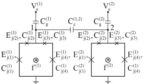
Figure 4: Two flux qubits $1$, $2$ are coupled via capacitance $Cc^{(1,2)}$. Each flux qubit is threaded by an external magnetic flux $f^{(l)}$, and we can control the energy bias of the qubit via the magnetic flux. Node $1$ and node $2$ represent the superconducting islands. JJ$2$ and JJ$3$ at each qubit have the same Josephson energies and capacitances that are $\alpha$ times larger than those of all remaining Josephson junctions. The electric potential of the island include node 1 (2) is $V_{i}^{(1)}$ $(V_{i}^{(2)})$.

The structure of each qubit is the same as that shown in Fig. 1. When we apply an external voltage $V_{e}^{(l)}$ on each qubit, the qubit interact with each other across the capacitor $C_{c}^{(1,2)}$. We describe the details of this circuit in the following subsections.

III.2 Hamiltonian

We now consider the electric energy and potential energy of the circuit in Fig. 4 as follows:

$$T = \frac{1}{2}\sum_{k=1}^{4}\sum_{l=1}^{2}{C}^{(l)}_{j(k)}\left(\frac{\Phi_{0}}{2\pi}\dot{\varphi}^{(l)}_{k}\right)^{2}$$ (5)

$$+\frac{1}{2}\sum_{l=1}^{2}{C}_{g}^{(l)}\left(V_{e}^{(l)}-V_{i}^{(l)}\right)^{2}$$

$$+\frac{1}{2}C_{c}^{(1,2)}\left(V_{i}^{(1)}-V_{i}^{(2)}\right)^{2}$$

$$U = \sum_{k=1}^{4}\sum_{l=1}^{2}{E}^{(l)}_{j(k)}\left(1-\cos\varphi^{(l)}_{k}\right)$$ (6)

$$H_{total} = T+U=\sum_{l=1}^{2}H_{A}^{(l)}+H_{B}$$ (7)

$$H_{A}^{(l)} = \frac{1}{2}\sum_{k=1}^{4}{C}^{(l)}_{j(k)}\left(\frac{\Phi_{0}}{2\pi}\dot{\varphi}^{(l)}_{k}\right)^{2}+\frac{1}{2}{C}_{g}^{(l)}\left(V_{e}^{(l)}-V_{i}^{(l)}\right)^{2}$$ (8)

$$+\sum_{k=1}^{4}{E}^{(l)}_{j(k)}\left(1-\cos\varphi^{(l)}_{k}\right)$$

$$H_{B} = \frac{1}{2}C_{c}^{(1,2)}\left(V_{i}^{(1)}-V_{i}^{(2)}\right)^{2}$$ (9)

where $C_{g}^{(l)}$, $f^{(l)}$, $V_{e}^{(l)}$, and $V_{i}^{(l)}$ denotes gate capacitance, external magnetic flux, applied external voltage, and the electric potential of the island including node $l$ for the $l$ th qubit respectively. Here, node $l$ represents the superconducting islands.

For an arbitrary $f$, we can derive the effective four-level Hamiltonian $\hat{H}_{ge}$ of the eigenspace spanned by $\lvert g_{l}\rangle$ and $\lvert e_{l}\rangle$ from $H_{total}$. Here, $\lvert g_{l}\rangle$ and $\lvert e_{l}\rangle$ correspond to the ground state and first excited state of the $l^{th}$ qubit without interactions for $f^{(1)}=f^{(2)}==0.5$. We expand $H_{total}$ by $\lvert g\rangle_{l}$ and $\lvert e\rangle_{l}$. The effective Hamiltonian $\hat{H}_{ge}$ becomes as follows:

$$\hat{H}_{ge} = \sum_{v_{1}\in(g_{1},e_{1}),v_{2}\in(g_{2},e_{2})}\lvert v_{1}v_{2}\rangle\langle v_{1}v_{2}\rvert\hat{H}_{total}\lvert v_{1}v_{2}\rangle\langle v_{1}v_{2}\rvert$$ (10)

$$= \sum_{l=1}^{2}\frac{1}{2}\left(\Delta^{(l)}\sigma_{Z}^{(l)}+\varepsilon^{(l)}\sigma_{Y}^{(l)}\right)+g\sigma_{Z}^{(1)}\sigma_{Z}^{(2)}$$

where $g$ denotes the Ising type interaction strength between qubit $1$ and $2$. We show the change of the qubit energy $E_{01}$ and the interaction strength $g$ as a function of applied voltages in Fig. 5.

Figure 5: The voltage dependence of the qubit energy $\Delta$ and the interaction strength $g$ between two qubits of the circuit in Fig. 4. Here, both of the gate capacitance $C_{g}^{l}=0.077$ fF, coupling capacitance $C_{c}=0.077$ fF.

Large interaction strength and small derivative of qubit energy against voltage can be achieved by the large coupling capacitance $Cc$ between each qubits. This seems to show that one can suppress errors by increasing $Cc$. We discuss about the errors during controlled-phase gate operation in following section.

III.3 Effects on interaction from change in electric field

To evaluate the performance of our scheme, we focus on two types of errors. Firstly, we analyze the dephasing errors due to the fluctuations of applied voltage. We define this type of error $\epsilon_{d}$ and dephasing time $T_{2}$ as follows:

$$\epsilon_{d} = \frac{t_{cp}}{T_{2}},t_{cp}=\frac{\pi}{4g},T_{2}=\frac{1}{|\frac{dE_{01}}{dv}|\delta v}$$ (11)

where we assume $t_{cp}<<T_{2}$. Here, $t_{cp}$ denotes the necessary time to perform a controlled-phase gate with Ising type interaction, $v$ denotes the external voltage of each qubit, and $\delta v$ denotes the fluctuation width of $v$. It is worth mentioning that $\epsilon_{d}$ has a linear relationship with $\delta v$. To make $\epsilon_{d}$ smaller, We should obtain a parameter set where the absolute value of the gradient of the qubit energy $E_{01}$ is small and the interaction strength $g$ is large.

Secondly, we investigate the jitter error of a two-qubit gate operation. The Ising type interaction can implement the controlled-phase gate

$$U_{CZ}^{(1,2)}(t) = \exp\left(-i4gt\frac{1+\sigma_{Z}^{(1)}}{2}\frac{1+\sigma_{Z}^{(2)}}{2}\right),$$ (12)

where $g$ denotes the interaction strength in Eq. (10), $t=\frac{\pi}{4g}$ denotes the time to apply voltages, and $U_{CZ}^{(1,2)}$ denotes a controlled-phase gate between qubit $1$ and $2$. By performing the controlled-phase gate on two qubits which are initialized to $\lvert++\rangle_{12}$ state, we can obtain the two-qubit cluster state. But, the applied voltages may not create the desired state due to error in the timing $t^{\prime}=t+\delta t$, where $\delta t$ is timing jitter. We introduce the controlled-phase gate $U_{CZ}^{(1,2)}(t)$ including the timing error to calculate a gate fidelity $F_{CZ}=|\langle\phi\lvert\phi^{\prime}\rangle|^{2}$ with

$$\lvert\phi\rangle=U_{CZ}^{(1,2)}(t)\lvert++\rangle,\lvert\phi^{\prime}\rangle=U_{CZ}^{(1,2)}(t^{\prime})\lvert++\rangle.$$ (13)

Here, we define the timing error $\epsilon_{tim}=1-F_{CZ}$, and the local error $\epsilon_{loc}(=\epsilon_{d}+\epsilon_{tim})$. We show the $\epsilon_{loc}$ against the applied voltage $V_{e}$ with the particular values of $Cc$ in Fig. 6.

Figure 6: The total local error $\epsilon_{loc}(=\epsilon_{d}+\epsilon_{tim})$ as a function of voltage with different coupling capacitance $Cc$. Here, we set the fluctuation width of voltage $\delta v=0.21$ $\mu$V and the timing jitter $\delta t=50$ psec. Dashed line denotes an error of $0.1$%.

The threshold of local errors for fault-tolerant quantum computation is known to be around 1%. Also, it is known that, if the error rate is close to the threshold, the necessary number of qubits for the computation drastically increases Raussendorf et al. (2007); Devitt et al. (2013). Therefore, we set the threshold to $\epsilon_{loc}=0.1$%. As shown in Fig. 5, we can increase the coupling strength $g$ by increasing $Cc$. Meanwhile, the strong coupling strength causes the large timing error. Therefore, as shown in Fig. 6, the optimal voltage exists for each of the $Cc$ which minimizes the total local error. In addition, by increasing $Cc$, the total error tends to be smaller. This result shows that the large $Cc$ has an advantage for quantum error correction against local errors. However, for multi-qubit systems, increasing $Cc$ causes a different problem. Unwanted interaction strength between non-nearest neighbor qubits increases due to the large $Cc$. For this reason, the $Cc$ should be set to be around $0.075$ fF. The detail of this will be discussed in Section IV.2.

IV Multi-qubit system

In this section, we generalize our scheme to multi-qubit system. Firstly, we discuss how to control the capacitive interactions between superconducting flux qubits via applied voltage. Secondly, we show how to apply our scheme to generate a two dimensional cluster state using superconducting flux qubits arranged on square lattice.

IV.1 Generating interaction between multi-qubits system

Here, we discuss the interactions between capacitively coupled $N$ flux qubits that are arranged in one dimensional line as shown in Fig. 7. For simplicity, we assume homogeneous flux qubits.

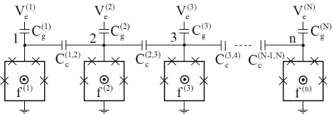
Figure 7: A flux qubit at the site $j(1<j<N)$ couples with the nearest neighbor qubits via capacitance $C_{c}^{(j,j\pm 1)}$. For simplicity, we assume homogeneous flux qubits. Each node $j$ represents the superconducting islands. Each qubit has four Josephson junctions. Two Josephson junctions directly connected to the node have the Josephson energies and capacitances that are $\alpha$ times larger than the other two Josephson junctions.

$f^{(j)}$ denotes the external magnetic flux through the loop of the $j$ th qubit. When all flux $f^{(j)}$ are $0.5$, the system Hamiltonian is described as follows.

$$\hat{H} = \sum_{l=1}^{N}\frac{1}{2}\Delta_{(l)}\sigma_{Z}^{(l)}+\sum_{l,l^{\prime}=1}^{N}g_{(|l-l^{\prime}|)}\sigma_{Z}^{(l)}\sigma_{Z}^{(l^{\prime})}$$ (14)

where $\Delta_{(l)}$ denotes the energy of the $l$ th qubit, $g_{(|l-l^{\prime}|)}$ denotes the interaction strength between each pair of qubits at a site $(l,l^{\prime})$, and $|l-l^{\prime}|$ denotes the site distance between these qubits (e.g. when qubit $l$ and $l^{\prime}$ are nearest neighbor pair, $|l-l^{\prime}|=1$.).

IV.2 Generation of a one dimensional cluster state

Non-nearest neighbor interactions cause spatially-correlated errors that are difficult to correct by quantum error correction. In this subsection, we show the way to evaluate this error. We define the ratio between nearest neighbor interaction $g(=g_{(1)})$ and next-nearest neighbor interaction $g_{(2)}$ as $R\left(=\frac{g_{(2)}}{g_{(1)}}\right)$ where all qubits are applied voltage $V_{e}$. We show that the interaction strength $g(|l-l^{\prime}|)$ decreases exponentially as the site distance $|l-l^{\prime}|$ increases, and the Ratio $R$ depends on the coupling capacitance $Cc$ between each qubit. This is a striking feature in our scheme using voltage for the control of the qubit-interaction, because the effect from any control lines can decrease only polynomially against the site distance if one uses magnetic field for the control. We show the interaction strengths of 6 qubits system as a function of $Cc$ in Fig. 8.

Figure 8: The $Cc$ dependence of the interaction strengths and the coupling ratio $R\left(=\frac{g_{(2)}}{g_{(1)}}\right)$ where $g(|l-l^{\prime}|)$ denotes the interaction strength between a pair of qubits at a site $(l-l^{\prime})$.

If we apply voltage on all qubits, interaction occurs between such qubits. The total error $\epsilon_{non}^{(j)}$ caused by non-nearest neighbor interactions on $j$ th qubit during controlled-phase operation is calculated as follows:

$$\epsilon_{non}^{(j)}=\sum_{n=2}^{N/2}g_{(n)}t_{cp}m_{(n)}=\sum_{n=2}^{N/2}\frac{\pi}{4}R^{(n-1)}m_{(n)}$$ (15)

where $n$ denotes the site distance between the $j$ th qubit and the coupled non-nearest neighbor qubits, $m_{(n)}^{(j)}$ denotes the number of such non-nearest qubits.

Such the existence of the spartially-correlated error will increase the threshold for quantum error correction Aharonov et al. (2006). Large capacitance tends to decrease local errors as shown in Fig. 6, while large capacitance induces more spartially-correlated errors as shown in Fig. 8. However, when we consider the spatially-correlated error, the error threshold value of the surface code is not well studied. Thus, we set the upper bound of the spatially-correlated error on each qubit $\epsilon_{non}\leq\frac{1}{10000}$ which is an order of magnitude smaller than the threshold of local error for surface coding scheme. If this condition is satisfied, we assume that spatially-correlated error is enough to perform a fault-tolerant quantum computation. When we apply voltage on all qubits to perform controlled-phase gates to all pairs of nearest neighbor qubit, a range of values that the coupling capacitance $Cc$ can take while satisfying the above condition is smaller than the proper range of $Cc$ discussed in Subsection III.3. Therefore, we do not apply voltage on all qubits but apply voltage on some of them. We choose pairs of nearest neighbor qubits that we will apply the voltage, and we set a site distance $p$ between the pairs. Then, if $R$ is small enough, $\epsilon_{non}$ of each qubit is the following equation:

$$\epsilon_{non}^{(j)}=\sum_{n=p}^{N/2}\frac{\pi}{4}R^{(n-1)}\leq\frac{1}{10000}$$ (16)

where $p$ is the site distance between qubits applied by voltage.

Since there are many parameters on the interaction Hamiltonian, it is difficult to find an optimum set of parameters that minimize both of local and spatially-correlated errors. Therefore, we fix the following parameters: $\alpha=0.2$, $\delta_{v}=0.21$ $\mu$V, $\delta_{t}=50$ psec. To determine a minimum site distance $p$ while suppressing the correlated errors to be under $0.01$ %, we show the $Cc$ and $V$ dependences of the errors with $p=4,5$ in Fig. 9.

Figure 9: (a)The $Cc$ dependence of the correlated errors. Dashed line corresponds to an error of $0.01$ %. (b)The $V$ dependence of the total errors. Dashed line corresponds to an error of $0.1$ %.

As shown in Fig. 9, when $p=4$, the $\epsilon_{non}$ exceeds $0.01$ % around $Cc=0.04$ fF. We cannot sufficiently suppress local errors using coupling capacitance smaller than $0.07$ as shown in Fig. 6. Thus, the site distance $p$ should be larger than $5$. Meanwhile, when $p=5$, the $\epsilon_{non}$ exceeds $0.01$ % around $Cc=0.09$ fF. Then the total error of the controlled-phase operation can be sufficiently suppressed to be less than $0.1$ % using the coupling capacitance $Cc$ around $0.077$ fF as shown in Fig. 9. Therefore, it is preferable that the site distance $p=5$ be selected. In order to adopt sufficiently large coupling capacitance such that the $\epsilon_{loc}$ below $0.1$ %, we need to choose sufficiently large $p$ such that the $\epsilon_{non}$ below $0.01$ %. We discuss about the way which can further reduce $p$ in the following.

The $p$ determines the maximum number of controlled-phase gates that are performed simultaneously on the same system. For example, we can perform $\lfloor\frac{N-2}{p+1}\rfloor+1$ controlled-phase gates in parallel using $N$-qubits one dimensional system. If we can use the smaller $p$ without adding extra errors, we can perform more controlled-phase gates in parallel. So that we can generate a cluster state within a shorter operating time. For this purpose, we introduce the spin echo technique where implementation of a $\pi$ pulse (single qubit $\sigma_{X}$ rotation) to the target qubit could refocus the dynamics of the spin so that effects of interactions on the target qubit should be cancelled out. We apply two $\pi$ pulses to pairs of qubits to suppress spatially-correlated errors. For example, we set three qubits in a raw and apply voltage $V_{e}^{(n)}$ to the $n$ th qubits $(n=1,2,3)$ as shown in Fig. 10, where $V_{e}^{(1)}$ and $V_{e}^{(2)}$ are equal, $V_{e}^{(3)}$ is an arbitrary voltage, and the strength of interaction between qubit $1$ and $2$ is $g$.

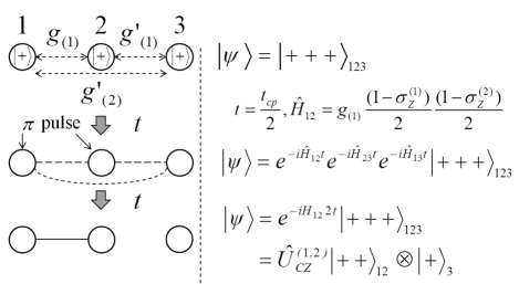
Figure 10: When we perform a $\pi$ pulse on qubit $1$ and $2$ at $t=t_{cp}/2$, the nearest neighbor interaction between qubit $2$ and $3$ and the non-nearest neighbor interaction between qubit $1$ and $3$ are cancelled out. In such way, we can perform controlled-phase gate without changing the state of other qubits.

We set each qubit to be prepared in $\lvert+\rangle$ state, let the state evolve for a time $t_{cp}/2$, perform two $\pi$ pulses to qubit $1$ and $2$, and let the state evolve for a time $t_{cp}/2$. The final state become as follows:

$$\hat{U}\lvert+++\rangle_{123} = \frac{1}{\sqrt{2}}\left(\lvert+0\rangle_{12}+\lvert-1\rangle_{12}\right)\otimes\lvert+\rangle_{3}.$$ (17)

Here, the interactions $g_{(1)}\sigma_{Z}^{(2)}\sigma_{Z}^{(3)}$ and $g_{(2)}\sigma_{Z}^{(1)}\sigma_{Z}^{(3)}$ are cancelled out due to the $\pi$ pulses and we obtain a cluster state between qubit $1$ and $2$.

This method can be applied with the case of arbitrary number of qubits. The general rules are follows: let us consider a pair of qubits. If we perform $\pi$ pulses on both of qubits, the interaction between them is not affected by these pulses. On the other hand, if we perform $\pi$ pulse on one of them, the interaction between them is cancelled out. These properties would be crucial for generating a cluster state as we will describe.

For generating a large one dimensional cluster state using $N$ qubits of the circuit in Fig. 7, we show the procedure as follows:

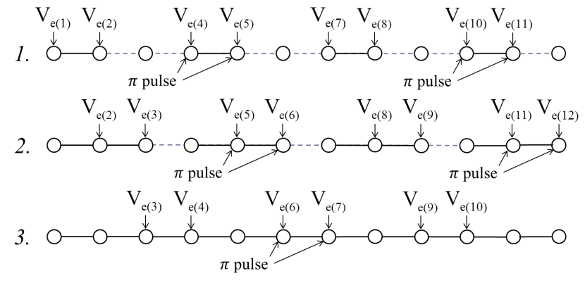
Figure 11: The $3$-step procedure for generating a one dimensional cluster state. Step 1. We initialize $3n-2$ th and $3n-1$ th qubits in $\lvert+\rangle$. Here, $n=1,2,\cdot\cdot,\lfloor\frac{N+1}{3}\rfloor$ where $\lfloor x\rfloor$ is the integer part of $x$. After that we apply voltage on $3n-2$ th and $3n-1$ th qubits. Let the state evolve for a time $\frac{t_{cp}}{2}$, perform $\pi$ pulses to $6n-2$ th and $6n-1$ th qubits, and let the state evolve for a time $\frac{t_{cp}}{2}$. After these operations, controlled-phase gates have been performed between qubit $3n-2$ and $3n-1$. Step 2. We initialize $3n$ th qubits in $\lvert+\rangle$. After that, similar to the Step 1, we perform controlled-phase gates between qubit $3n-1$ and $3n$. Step 3. We initialize $3n+1$ th qubits in $\lvert+\rangle$. After that, similar to the Step 1 and 2, we perform controlled-phase gates between qubit $3n$ and $3n+1$.

Step 1

We apply voltage to $(3n-2)$ th and $(3n-1)$ th qubit for performing controlled-phase gates between $(3n-2)$ th and $(3n-1)$ th qubit where $n=1,2,\cdot\cdot,\lfloor\frac{N+1}{3}\rfloor$.

Step 2

We apply voltage to $(3n-1)$ th and $3n$ th qubit for performing controlled-phase gates between $(3n-1)$ th and $3n$ th qubit where $n=1,2,\cdot\cdot,\lfloor\frac{N+1}{3}\rfloor$.

Step 3

We apply voltage to $3n$ th and $\left(3n+1\right)$ th qubit for performing controlled-phase gates between $(3n-1)$ th and $3n$ th qubit where $n=1,2,\cdot\cdot,\lfloor\frac{N+1}{3}\rfloor$.

At each step of the above procedure, $\lfloor\frac{N-1}{3}\rfloor$ controlled-phase gate are performed in parallel. At each step, we will perform the following procedure to perform the controlled-phase gate. Firstly, prepare the qubit state in $\lvert+\rangle$. Secondly, let the state evolve for a time $t=\frac{t_{cp}}{2}$ according to the Hamiltonian described in Eq. 14. Thirdly, perform the $\pi$ pulses to suppress the non-local interaction. Finally, let the state evolve for a time $t=t_{cp}$. We show the details of these operations in Fig. 11 and explain how the non-local interaction is suppressed in Fig. 12.

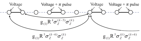
Figure 12: The influence of non-local interactions. During the controlled-phase gate, each target qubit are affected by non-local interactions. We show the strength of mainly three non-local interactions with $k$ th qubit. These interactions are not cancelled out by $\pi$ pulses.

When all coupling capacitance are $Cc\leq 0.077$ fF, the spatially-correlated error on each qubits become as follows:

$$\epsilon_{non}^{(j)}\!=\!\sum_{n=5}^{N/2}\frac{\pi}{4}R^{(n-1)}m_{(n)}\!\simeq\!\frac{\pi}{4}(R^{4}+2R^{5})\!\leq\!\frac{1}{10000}.$$ (18)

The $k$ th qubit is affected by mainly three non-local interactions as shown in Fig. 12. The strength of the largest interaction is $gR^{4}$, and the strength of the other two interactions are $gR^{5}$. The remaining non-local interactions are negligibly small.

IV.3 Generation of a two dimensional cluster state

Next, we show how to generate a two dimensional cluster state using $N^{2}$ flux qubits arranged on $N\times N$ square lattice. We show a part of the circuit in Fig. 13.

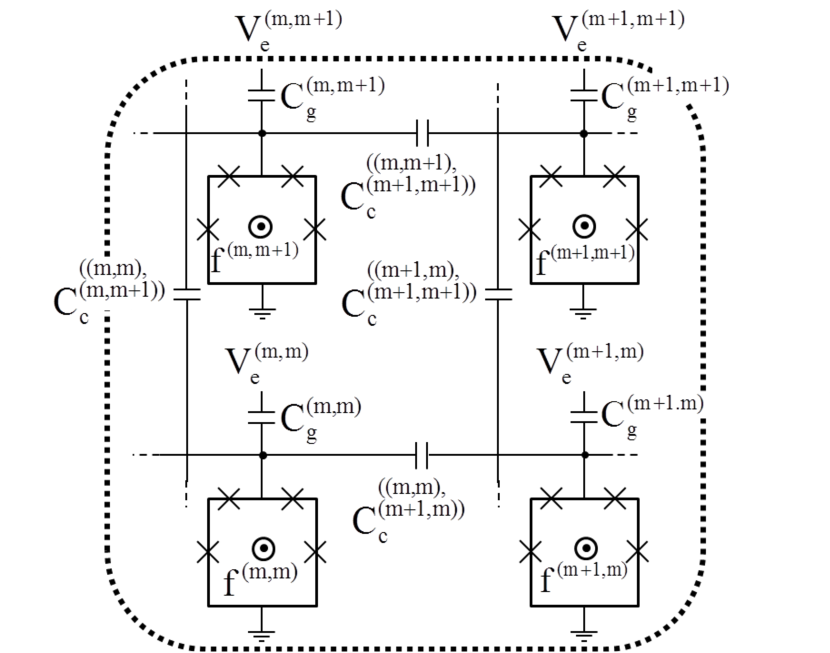
Figure 13: Physical circuit for generating a two dimensional cluster state. These four qubits correspond to the qubits surrounded by dot line in Fig. 14. Two Josephson junctions directly connected to a node (the superconducting islands) have the Josephson energies and capacitances that are $\alpha$ times larger than the other two Josephson junctions. Every flux qubit at site (j,k) couples with the four nearest neighbor qubits via capacitance $Cc^{((j,k)(j\pm 1,k\pm 1))}$.

$f^{(j,k)}$ denotes the external magnetic flux through the loop of the qubit at site $(j,k)$. Here, $(j,k)$ corresponds to the lattice point. When all flux $f^{(j,k)}$ are $0.5$, the system Hamiltonian is described as follows:

$$\hat{H} = \sum_{(l,m)}\frac{\Delta^{(l,m)}}{2}\sigma_{Z}^{(l,m)}$$ (19)

$$+\sum_{((l,m),(l^{\prime},m^{\prime}))}g_{(|l-l^{\prime}|+|m-m^{\prime}|)}\sigma_{Z}^{(l,m)}\sigma_{Z}^{(l^{\prime},m^{\prime})}$$

where $\Delta_{(l,m)}$ denotes the energy of the qubit at site $(l,m)$, $g_{(|l-l^{\prime}|+|m-m^{\prime}|)}$ denotes the interaction strength between each pair of qubits at site $(l,m)$ and $(l^{\prime},m^{\prime})$, and $|l-l^{\prime}|+|m-m^{\prime}|$ denotes the site distance between these qubits.

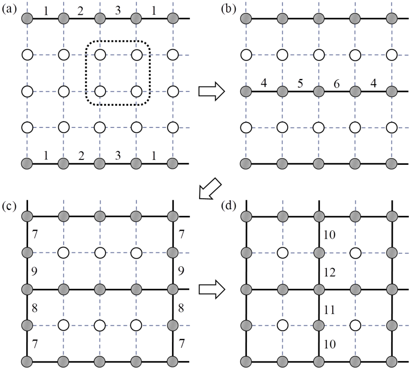
Figure 14: Schematic of our procedure for generating a two dimensional cluster state by graph state representation. Circles correspond to qubits, dashed lines correspond to electrically connection via a capacitance, solid-lines correspond to entanglement between qubits, and numbers show the order in which controlled-phase gates are performed by our procedure. White circles denote separable qubit, and gray circles denote qubits constituent of cluster state(s).

Here, we show the 12-step procedure as follows for generating a two dimensional cluster state.

Step 1-3

We perform $(N-1)\lfloor\frac{N}{4}\rfloor$ controlled-phase gate to generate $\lfloor\frac{N}{4}\rfloor$ one dimensional cluster states using qubits located in the $4m-3(m=1,2,\cdot\cdot,\lfloor\frac{N+3}{4}\rfloor)$ row in the same way as shown in Fig. 11. Then the spatially-correlated error of each qubit in the $4m-3$ row is smaller than $\frac{1}{10000}$. We show the outline of these steps in Fig. 14(a).

Step 4-6

We perform $(N-1)\lfloor\frac{N-2}{4}\rfloor$ controlled-phase gate to generate $\lfloor\frac{N-2}{4}\rfloor$ one dimensional cluster states using qubits located in the $4p-1(p=1,2,\cdot\cdot,\lfloor\frac{N+1}{4}\rfloor)$ row in the same way as above. We show the outline of these steps in Fig. 14(b).

Step 7-9

We perform $(N-1)\lfloor\frac{N}{4}\rfloor$ controlled-phase gate to generate a two dimensional graph state as shown in Fig. 14(c) using qubits located in the $4m-3$ column across $\lfloor\frac{N}{2}\rfloor$ one dimensional cluster states. We show the outline of these steps in Fig. 14(c).

Step 10-12

We perform $(N-1)\lfloor\frac{N-2}{4}\rfloor$ controlled-phase gate to generate a two dimensional cluster states using qubits located in the $4p-1$ column. We show the outline of these steps in Fig. 14(d).

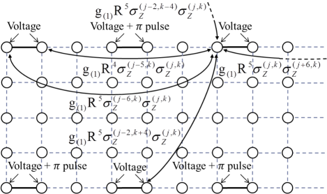
Figure 15: Operations and the influence of non-local interactions in generating a two dimensional cluster state. In this step, we apply voltage to qubit at site $(3n-2,4m-3)$ and $(3n-1,4m-3)$. Let the state evolve for a time $\frac{t_{cp}}{2}$, perform $\pi$ pulses to qubit at site $(6n^{\prime}-5,8m^{\prime}-7)$, $(6n^{\prime}-4,8m^{\prime}-7)$, $(6n^{\prime}-2,8m^{\prime}-3)$, and $(6n^{\prime}-1,8m^{\prime}-3)$, and let the state evolve for a time $\frac{t_{cp}}{2}$. So that controlled-phase gates can be implemented between the pair of qubits at site $(3n-2,4m-3)$ and $(3n-1,4m-3)$. Here, $m=1,2,\cdot\cdot,\lfloor\frac{N+3}{4}\rfloor$, $m^{\prime}=1,2,\cdot\cdot,\lfloor\frac{N+3}{8}\rfloor$, $n=1,2,\cdot\cdot,\lfloor\frac{N+1}{3}\rfloor$, and $n^{\prime}=1,2,\cdot\cdot,\lfloor\frac{N+1}{6}\rfloor$. Each target qubit is affected by non-local interactions from qubits on the same row and other rows. We show mainly five non-local interactions with the qubit at site (j,k). These interactions are not cancelled out by $\pi$ pulse.

We show the details of each step of above procedure for generating a two dimensional cluster state in Fig. 15. During each step, a part of the non-local interactions are not cancelled out by $\pi$ pulses. When all coupling capacitance are $Cc\leq 0.077$ fF, the spatially-correlated error on each qubits become as follows:

$$\epsilon_{non}^{(j,k)}\!=\!\sum_{n=5}^{N/2}\frac{\pi}{4}R^{(n-1)}m_{(n)}\!\simeq\!\frac{\pi}{4}(R^{4}\!+\!4R^{5})\!\leq\!\frac{1}{10000}.$$ (20)

The qubit at site $(j,k)$ is affected by mainly five non-local interactions as shown in Fig. 15. The strength of the largest interaction is $g_{(1)}R^{4}$, and the strength of the other four interactions are $g_{(1)}R^{5}$. The remaining non-local interactions are negligibly small.

V Conclusion

In conclusion, we suggest a new way to generate Ising interaction between capacitively-coupled superconducting flux qubits by using an applied voltage, and we also show architecture about how to make a two-dimensional cluster state in this coupling scheme. Unlike the standard schemes, our scheme does not require to change the applied magnetic field on the flux qubit for the control of the interaction. Since applying local voltages is typically much easier than applying local magnetic flux, the scheme described in this paper may have advantage to perform two-qubit gates on target qubits without affecting any other qubits. Our result paves the way for scalable quantum computation with superconducting flux qubits.

References

- Chen et al. (2007) G. Chen, Z. Chen, L. Yu, and J. Liang, Phys. Rev. A 76, 024301 (2007).
- Padurariu and Nazarov (2010) C. Padurariu and Y. V. Nazarov, Phys. Rev. B 81, 144519 (2010).
- (3) P.-M. Billangeon et al., Private communication.
- Chiorescu et al. (2003) I. Chiorescu, Y. Nakamura, C. M. Harmans, and J. Mooij, Science 299, 1869 (2003).
- Niskanen et al. (2006) A. Niskanen, K. Harrabi, F. Yoshihara, Y. Nakamura, and J. Tsai, Physical Review B 74, 220503 (2006).
- Bylander et al. (2011a) J. Bylander, S. Gustavsson, F. Yan, F. Yoshihara, K. Harrabi, G. Fitch, D. G. Cory, Y. Nakamura, J.-S. Tsai, and W. D. Oliver, Nature Physics 7, 565 (2011a).
- Yoshihara et al. (2014) F. Yoshihara, Y. Nakamura, F. Yan, S. Gustavsson, J. Bylander, W. D. Oliver, and J.-S. Tsai, Phys. Rev. B 89, 020503 (2014).
- Ansmann et al. (2009) M. Ansmann, H. Wang, R. C. Bialczak, M. Hofheinz, E. Lucero, M. Neeley, A. O’Connell, D. Sank, M. Weides, J. Wenner, et al., Nature 461, 504 (2009).
- Hofheinz et al. (2009) M. Hofheinz, H. Wang, M. Ansmann, R. C. Bialczak, E. Lucero, M. Neeley, A. O’Connell, D. Sank, J. Wenner, J. M. Martinis, et al., Nature 459, 546 (2009).
- Steffen et al. (2006) M. Steffen, M. Ansmann, R. C. Bialczak, N. Katz, E. Lucero, R. McDermott, M. Neeley, E. M. Weig, A. N. Cleland, and J. M. Martinis, Science 313, 1423 (2006).
- DiCarlo et al. (2009) L. DiCarlo, J. Chow, J. Gambetta, L. S. Bishop, B. Johnson, D. Schuster, J. Majer, A. Blais, L. Frunzio, S. Girvin, et al., Nature 460, 240 (2009).
- Koch et al. (2007) J. Koch, T. M. Yu, J. Gambetta, A. A. Houck, D. I. Schuster, J. Majer, A. Blais, M. H. Devoret, S. M. Girvin, and R. J. Schoelkopf, Phys. Rev. A 76, 042319 (2007).
- Manucharyan et al. (2009) V. E. Manucharyan, J. Koch, L. I. Glazman, and M. H. Devoret, Science 326, 113 (2009).
- Zhu et al. (2013) G. Zhu, D. G. Ferguson, V. E. Manucharyan, and J. Koch, Phys. Rev. B 87, 024510 (2013).
- You et al. (2007) J. You, X. Hu, S. Ashhab, and F. Nori, Physical Review B 75, 140515 (2007).
- Steffen et al. (2010) M. Steffen, F. Brito, D. DiVincenzo, M. Farinelli, G. Keefe, M. Ketchen, S. Kumar, F. Milliken, M. B. Rothwell, J. Rozen, et al., Journal of Physics: Condensed Matter 22, 053201 (2010).
- Barends et al. (2013) R. Barends, J. Kelly, A. Megrant, D. Sank, E. Jeffrey, Y. Chen, Y. Yin, B. Chiaro, J. Mutus, C. Neill, P. O’Malley, P. Roushan, J. Wenner, T. C. White, A. N. Cleland, and J. M. Martinis, Phys. Rev. Lett. 111, 080502 (2013).
- Ghosh et al. (2013) J. Ghosh, A. Galiautdinov, Z. Zhou, A. N. Korotkov, J. M. Martinis, and M. R. Geller, Phys. Rev. A 87, 022309 (2013).
- Chen et al. (2014) Y. Chen, C. Neill, P. Roushan, N. Leung, M. Fang, R. Barends, J. Kelly, B. Campbell, Z. Chen, B. Chiaro, A. Dunsworth, E. Jeffrey, A. Megrant, J. Y. Mutus, P. J. J. O’Malley, C. M. Quintana, D. Sank, A. Vainsencher, J. Wenner, T. C. White, M. R. Geller, A. N. Cleland, and J. M. Martinis, Phys. Rev. Lett. 113, 220502 (2014).
- Geller et al. (2014) M. R. Geller, E. Donate, Y. Chen, C. Neill, P. Roushan, and J. M. Martinis, arXiv preprint arXiv:1405.1915 (2014).
- Sete et al. (2013) E. Sete, A. Galiautdinov, E. Mlinar, J. Martinis, and A. Korotkov, Phys. Rev. Lett. 110, 210501 (2013).
- Hover et al. (2014) D. Hover, S. Zhu, T. Thorbeck, G. Ribeill, D. Sank, J. Kelly, R. Barends, J. M. Martinis, and R. McDermott, Applied Physics Letters 104, 152601 (2014).
- Jeffrey et al. (2014) E. Jeffrey, D. Sank, J. Y. Mutus, T. C. White, J. Kelly, R. Barends, Y. Chen, Z. Chen, B. Chiaro, A. Dunsworth, A. Megrant, P. J. J. O’Malley, C. Neill, P. Roushan, A. Vainsencher, J. Wenner, A. N. Cleland, and J. M. Martinis, Phys. Rev. Lett. 112, 190504 (2014).
- Barends et al. (2014) R. Barends, J. Kelly, A. Megrant, A. Veitia, D. Sank, E. Jeffrey, T. White, J. Mutus, A. Fowler, B. Campbell, et al., Nature 508, 500 (2014).
- Bylander et al. (2011b) J. Bylander, S. Gustavsson, F. Yan, F. Yoshihara, K. Harrabi, G. Fitch, D. G. Cory, Y. Nakamura, J.-S. Tsai, and W. D. Oliver, Nature Physics 7, 565 (2011b).
- Stern et al. (2014) M. Stern, G. Catelani, Y. Kubo, C. Grezes, A. Bienfait, D. Vion, D. Esteve, and P. Bertet, Phys. Rev. Lett. 113, 123601 (2014).
- Plourde et al. (2004) B. L. T. Plourde, J. Zhang, K. B. Whaley, F. K. Wilhelm, T. L. Robertson, T. Hime, S. Linzen, P. A. Reichardt, C.-E. Wu, and J. Clarke, Phys. Rev. B 70, 140501 (2004).
- Grajcar et al. (2006) M. Grajcar, Y.-x. Liu, F. Nori, and A. M. Zagoskin, Phys. Rev. B 74, 172505 (2006).
- Hime et al. (2006) T. Hime, P. Reichardt, B. Plourde, T. Robertson, C.-E. Wu, A. Ustinov, and J. Clarke, science 314, 1427 (2006).
- van der Ploeg et al. (2007) S. H. W. van der Ploeg, A. Izmalkov, A. M. van den Brink, U. Hübner, M. Grajcar, E. Il’ichev, H.-G. Meyer, and A. M. Zagoskin, Phys. Rev. Lett. 98, 057004 (2007).
- Niskanen et al. (2007) A. Niskanen, K. Harrabi, F. Yoshihara, Y. Nakamura, S. Lloyd, and J. Tsai, Science 316, 723 (2007).
- Harris et al. (2007) R. Harris, A. Berkley, M. Johnson, P. Bunyk, S. Govorkov, M. Thom, S. Uchaikin, A. Wilson, J. Chung, E. Holtham, et al., Physical review letters 98, 177001 (2007).
- Ashhab et al. (2008) S. Ashhab, A. Niskanen, K. Harrabi, Y. Nakamura, T. Picot, P. De Groot, C. Harmans, J. Mooij, and F. Nori, Physical Review B 77, 014510 (2008).
- Yamamoto et al. (2008) T. Yamamoto, M. Watanabe, J. You, Y. A. Pashkin, O. Astafiev, Y. Nakamura, F. Nori, and J. Tsai, Physical Review B 77, 064505 (2008).
- Groszkowski et al. (2011) P. Groszkowski, A. G. Fowler, F. Motzoi, and F. K. Wilhelm, Phys. Rev. B 84, 144516 (2011).
- Siddiqi et al. (2006) I. Siddiqi, R. Vijay, M. Metcalfe, E. Boaknin, L. Frunzio, R. Schoelkopf, and M. Devoret, Physical Review B 73, 054510 (2006).
- Siddiqi et al. (2004) I. Siddiqi, R. Vijay, F. Pierre, C. M. Wilson, M. Metcalfe, C. Rigetti, L. Frunzio, and M. H. Devoret, Phys. Rev. Lett. 93, 207002 (2004).
- Jordan and Smith (2007) D. W. Jordan and P. Smith, Nonlinear ordinary differential equations: an introduction for scientists and engineers (New York, 2007).
- Kakuyanagi et al. (2013) K. Kakuyanagi, S. Kagei, R. Koibuchi, S. Saito, A. Lupaナ歡u, K. Semba, and H. Nakano, New Journal of Physics 15, 043028 (2013).
- Raussendorf et al. (2007) R. Raussendorf, J. Harrington, and K. Goyal, New Journal of Physics 9, 199 (2007).
- Devitt et al. (2013) S. J. Devitt, A. M. Stephens, W. J. Munro, and K. Nemoto, Nature communications 4 (2013).
- Aharonov et al. (2006) D. Aharonov, A. Kitaev, and J. Preskill, Phys. Rev. Lett. 96, 050504 (2006).