Abstract

We discuss the use of a class of exact finite energy solutions to the vacuum source-free Maxwell equations as models for multi- and single cycle laser pulses in classical interaction with relativistic charged point particles. These compact solutions are classified in terms of their chiral content and their influence on particular charge configurations in space. The results of such classical interactions motivate a phenomenological quantum description of a propagating laser pulse in a medium in terms of an effective quantum Hamiltonian.

PACS numbers:  03.50.De, 42.50.Ct, 42.55.Ah,

1 Introduction

Advances in laser technology have made possible the exploration of physical processes on unprecedented temporal and spatial scales. They have also opened up new possibilities for accelerating charged particles using laser-matter interactions. Multi- and single cycle high intensity ($10^{10}-10^{15}\,\text{W}\text{cm}^{-2}$) laser pulses can be produced using Q-switching or mode-locking techniques [1]. Pulses of even higher intensity ($\sim 10^{21}\,\text{W}\text{cm}^{-2}$) could accelerate charged particles such as electrons to relativistic speeds where radiation reaction and quantum effects may influence their dynamics [2]. Lower intensity pulses have also been used as diagnostic tools for exploring the structure of plasmas in various states [3, 4]. In order to interpret experimental data involving classical laser interactions with both charged and neutral matter, theoretical models [5, 6, 7, 8] rely crucially on parameterizations of the electromagnetic fields in laser pulses, particularly in situations where traditional formulations using monochromatic or paraxial-beam approximations have limitations [9, 10, 11]. Such theoretical models may not be compact in all spatial dimensions and the role of a laser pulse as a classical probe is further limited by the scales that it is designed to resolve. Pulse shape design characteristics are often guided by simulations of laser-matter interactions which incorporate the known laws of physics of relevance at such scales. For example, the intense experimental activity currently exploring the electromagnetic properties of single-cycle laser pulses with nanoscale objects (such as dielectric and plasmonic nanoparticles) demands efficient modelling tools that accommodate the spatial compactness of such pulses. Such tools will eventually require incorporation of quantum effects associated with these interactions in order to properly describe observations and yield practical applications involving nanostructured dielectrics and plasmonic metals [12]. Furthermore an effective quantum description of the laser pulse itself would offer a new simulation tool for designing more accurate methods of encoding quantum information.

The quanta associated with plane time-harmonic electromagnetic fields in vacuo provide ideal discrete two-state systems (photons) that are routinely used as controllable qubits in information science. Three-level bosonic quantum systems composed of two photons in the same spatial and temporal configuration have also been contemplated [13] in attempts to construct more efficient quantum gates for quantum communication. If one regards a free propagating classical single-cycle (therefore non-time-harmonic) laser pulse in vacuo as a spatially compact classical electromagnetic configuration with definite energy ${\cal{E}}$ and temporal width $t_{0}$, one expects that when ${\cal{E}}t_{0}\lesssim\hbar$ its dynamical evolution, in both vacuo and material media, should be controlled by an effective quantum Hamiltonian, rather than a classical one as is done in [14]. Such quantized collective states could then be entangled with other quantized pulses or free photon states and their interaction with classical or quantized states of electrically neutral continua (e.g. optically inhomogeneous and anisotropic dielectrics or plasmas) or charged matter (e.g. trapped ions [13]) may be worthy of investigation for technological applications such as quantum computing and encryption.

In this article we first discuss a viable methodology for parameterizing a particular class of propagating solutions to the source-free classical Maxwell equations in vacuo that offers an efficient means to explore the classical effects of compact laser pulses on free electrons in dynamical regimes where quantum effects are absent. The parameterization is constructed from a remarkable class of explicit solutions of the scalar wave equation found by Ziolkowski [15, 16, 17, 18, 19] following pioneering work by Brittingham [20] and Synge [21]. Solutions in this class are parameterized in terms of three real constants that are sufficient to completely determine the characteristics of any freely propagating laser pulse in full accord with Maxwell’s equations in free space. They describe solutions with finite total electromagnetic energy, electromagnetic fields bounded in all three spatial directions and experimentally distinguishable chiral configurations. With simple analytic structures their diffractive properties can be readily calculated together with the behaviour of relativistic charged particle-pulse interactions over a broad parameter range without recourse to expensive numerical computation. Based on this behaviour and by analogy with the effective Hamiltonian theory of diatomic molecules, we are led to construct a Hilbert space on which to describe certain quantum states of an electromagnetic pulse undergoing unitary evolution generated by an effective phenomenological quantum Hamiltonian in a medium. Such a Hamiltonian, defined in terms of a set of parameters associated with its medium interaction, serves as an effective quantum model for the quantum pulse evolution.

2 Parameterizing Compact Electromagnetic Laser Pulses

If a complex scalar field $\alpha$ satisfies $\Box\,\alpha=0$ and $\Pi_{\mu\nu}$ is any covariantly constant (degree 2) anti-symmetric tensor field on spacetime (i.e. $\Pi_{\mu\nu;\delta}=0$ for all $\mu,\nu,\delta=0,1,2,3$), then the complex tensor field $F_{\mu\nu}=\partial_{\mu}A_{\nu}-\partial_{\nu}A_{\mu}$ satisfies the source-free Maxwell equations in vacuo with:

$$A_{\nu} = \partial_{\gamma}\left(\alpha\,\,\Pi_{\mu\beta}\right)\,\epsilon^{\gamma\mu\beta}{}_{\nu}\,\sqrt{|g|}$$ (1)

where $|g|$ is the modulus of the determinant of the spacetime metric tensor field $g$ with components $g_{\mu\nu}$ and $\epsilon^{\gamma\mu\beta}{}_{\nu}\,$ denotes the Levi-Civita alternating symbol. In the following, we restrict to Minkowski spacetime, in which case the components $\Pi_{\mu\nu}$ can be used to encode three independent Hertz vector fields and their duals.

General solutions to $\Box\,\alpha=0$ can be constructed by Fourier analysis. In cylindrical polar Minkowski coordinates $\{t,r,z,\theta\}$, axially symmetric solutions propagating along the $z$-axis have, for $z\geq 0$, the double integral representation $\alpha(t,r,z)=\int_{-\infty}^{\infty}\,d\omega\,e^{-i\omega t}\widetilde{\alpha}(\omega,r,z)$ where:

$$\widetilde{\alpha}(\omega,r,z) = \int_{0}^{\frac{\omega}{c}}k\,f_{\omega}(k)J_{0}(kr)e^{\pm iz\sqrt{(\frac{\omega}{c})^{2}-k^{2}}}\,dk+\int_{\frac{\omega}{c}}^{\infty}kf_{\omega}(k)J_{0}(kr)e^{-z\sqrt{k^{2}-(\frac{\omega}{c})^{2}}}\,dk$$

in terms of the zero order Bessel function and the speed of light in vacuo $c$.

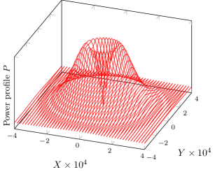
Figure 1: Power profile $P$ of the $(\text{CM},1)$ laser pulse at $Z=0,\,T=0$ with parameters $\{\Lambda=600,\Psi_{1}=1,\Psi_{2}=1000,\Phi=0.001,\Xi=1\}$

Conditions on the Fourier amplitudes $f_{\omega}(k)$ can be given so that the Hertz procedure above gives rise to real singularity free electromagnetic fields with finite total electromagnetic energy. A particularly simple class of pulses that can be generated in this way follows from the complex axi-symmetric scalar solution:

$$\alpha(t,r,z) = \frac{\ell_{0}^{2}}{r^{2}+(\psi_{1}+i(z-ct))\,(\psi_{2}-i(z+ct))}$$ (2)

where $\ell_{0},\psi_{1},\psi_{2}$ are strictly positive (real) parameters with physical dimensions of length. The relative sizes of $\psi_{1}$ and $\psi_{2}$ determine both the direction of propagation along the $z-$axis of the dominant maximum of the pulse profile. When $\psi_{1}\gg\psi_{2}$, the dominant maximum propagates along the $z-$axis to the right. The parameter $\ell_{0}$ determines the magnitude of such a maximum. The structure of such solutions has been extensively studied in [22, 23] in conjunction with particular choices of $\Pi_{\mu\nu}$ together with generalizations discussed in [24, 25].

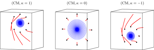
Figure 2: Three-dimensional spacecurves for particles subject to an incident $(\text{CM},1)$ laser pulse (left), $(\text{CM},0)$ laser pulse (centre) and $(\text{CM},-1)$ laser pulse (right) with parameters $\{\Lambda=600,\Psi_{1}=1,\Psi_{2}=1000,\Phi=0.001,\Xi=1\}$. Each particle has initial velocity $\{\dot{R}(0)=0,\dot{\theta}(0)=0,\dot{Z}(0)=\frac{1}{200}\}$. The shaded circular disc region indicates the initial spot size ($R=10000$ for $(\text{CM},\pm 1)$ laser pulses and $R=20000$ for a $(\text{CM},0)$ laser pulse) relative to the black markers on the spacecurves that denote the initial positions of the charged test particles.

In general the six anti-symmetric tensors with components $\delta^{\mu}_{[\gamma}\delta^{\nu}_{\sigma]}$ in a Minkowski Cartesian coordinate system are covariantly constant and can be used to construct a complex eigen-basis of antisymmetric chiral tensors $\Pi^{s,\,\kappa}$, with $s\in\{\text{CE},\text{CM}\}$ and $\kappa\in\{-1,0,1\}$, satisfying

$${\cal O}_{z}\,\Pi^{s,\,\kappa} = \kappa\,\Pi^{s,\,\kappa}$$ (3)

where the operator ${\cal O}_{z}$ represents $\theta$ rotations about the $z-$axis generated by $-i\partial_{\theta}$ on tensors. These in turn can be used to construct a complex basis of chiral eigen-Maxwell tensor fields $F^{s,\,\kappa}_{\mu\nu}$. The index $s$ indicates that the CE (CM) chiral family contain electric (magnetic) fields that are orthogonal to the $z-$axis when $\kappa=0$. The chiral eigen-fields $F^{s,\,0}_{\mu\nu}$ inherit the axial symmetry of $\alpha(t,r,z)$ while those with $\kappa=\pm 1$ do not. The directions of electric and magnetic fields in any of these Maxwell solutions depend on their location in the pulse and the concept of a pulse polarisation is not strictly applicable. The chiral content as defined here can be used in its place. Non-chiral (complex) pulse configurations can be constructed by superposition: $F_{\mu\nu}=\sum_{s}\,\sum_{\kappa}F^{s,\,\kappa}_{\mu\nu}\,{\cal C}^{s,\,\kappa}$ with arbitrary constant complex coefficients ${\cal C}^{s,\,\kappa}$.

The energy, linear and angular momentum of the pulse in vacuo can be calculated from the components $T_{\mu\nu}$ of the Maxwell stress-energy tensor $T_{\mu\nu}=-\frac{1}{4}g_{\mu\nu}{\cal F}^{\alpha\beta}{\cal F}_{\alpha\beta}-{\cal F}_{\mu\alpha}{\cal F}^{\alpha}{}_{\nu}$ where ${\cal F}_{\mu\nu}=\text{Re}(F_{\mu\nu})$. If $\mathbf{e}$ and $\mathbf{b}$ denote time-dependent real electric and magnetic 3-vector fields associated with any pulse solution $F_{\mu\nu}$, its total electromagnetic energy $\mathcal{J}$, for a fixed set of parameters and any $z$, is calculated from

$$\mathcal{J} = \frac{1}{\mu_{0}}\int_{-\infty}^{\infty}\,dt\,\int_{S}({\mathbf{e}}\times{\mathbf{b}})\cdot d{\mathbf{S}}$$ (4)

where $S$ can be any plane with constant $z=z_{0}>0$. For spatially compact pulse fields in vacuo this coincides with the total pulse electromagnetic energy

$${\cal E} = \int_{\cal V}\rho\,d{\cal V}\,=\,\int_{-\infty}^{\infty}\!\!dz\,\int_{0}^{2\pi}\!\!d\theta\,\int_{0}^{\infty}\!\!rdr\;\rho(t,r,z,\theta)$$ (5)

where $\rho\equiv\frac{1}{2}\,\left(\epsilon_{0}\,{\mathbf{e}}\cdot{\mathbf{e}}+\frac{{\mathbf{b}}\cdot{\mathbf{b}}}{\mu_{0}}\right)$ is integrated over all space ${\cal V}$. This follows since $\nabla\cdot({\mathbf{e}}\times{\mathbf{b}})=-\mu_{0}\,\partial_{t}\,\rho$. To correlate $\mathcal{J}$ with other laser pulse properties and the choice of parameters, we bring the pulses $F^{s,\kappa}_{\mu\nu}$ for various values of $s$ and $\kappa$ into classical interaction with one or more charged point particles. The world-line in spacetime of a single particle, parameterized in arbitrary coordinates as $x^{\mu}=\xi^{\mu}(\tau)$ with a parameter $\tau$, is taken as a solution of the coupled non-linear differential equations

$${{\cal A}_{\mu}(\tau)} = \frac{q}{m_{0}c^{2}}{\cal F}_{\mu\nu}(\frac{}{}\!\xi(\tau))\,V^{\nu}(\tau)$$ (6)

in terms of the particle charge $q$ and rest mass $m_{0}$, for some initial conditions $\xi(0),V(0)$, where the particle 4-velocity satisfies $V^{\nu}\,V_{\nu}=-1$ and its 4-acceleration is expressed in terms of the Christoffel symbols $\Gamma^{\delta}{}^{\beta}{}_{\mu}$ as ${\cal A}_{\mu}(\tau)=\partial_{\tau}\,{V_{\mu}}(\tau)+V_{\delta}(\tau)\,V_{\beta}(\tau)\,\Gamma^{\delta}{}^{\beta}{}_{\mu}(\xi(\tau))$. In the following, radiation reaction and inter-particle forces are assumed negligible. From the solution $\xi(\tau)$ one can determine the increase (or decrease) in the relativistic kinetic energy transferred from the electromagnetic pulse to any particle and the nature of its trajectory in the laboratory frame for different choices of $s$ and $\kappa$.

3 Interactions of Compact Laser Pulses with Matter

The analysis of the previous section can be used to investigate the behaviour of a classical laser pulse interacting with electrically charged matter and motivates a model for a quantum laser pulse interacting with electrically neutral matter.

In order to facilitate the classical behaviour, we reduce the above equations of motion to dimensionless form and fix the physical dimensions of the fields involved. The Minkowski metric tensor field $g=g_{\mu\nu}dx^{\mu}\,dx^{\nu}$ (with $g_{\mu\nu}=\mathrm{diag}(-1,1,1,1)$) in inertial coordinates $x^{0}=ct,x^{1}=x,x^{2}=y,x^{3}=z$) has SI physical dimensions $[L]^{2}$. The SI dimension of electromagnetic quantities follows by assigning to $\epsilon_{0}F_{\mu\nu}\,dx^{[\mu}dx^{\nu]}$ in any coordinate system the physical dimension of charge. Furthermore, in terms of Minkowski polar coordinates $\{t,r,z,\theta\}$, introduce (for ease of graphical visualization) the dimensionless coordinates $\{R=r/\Phi\ell_{0},\,T=ct/\ell_{0},\,Z=z/\Xi\ell_{0}\}$ and real dimensionless parameters $\Lambda,\Psi_{j}=\psi_{j}/\ell_{0}$ ($j=1,2$) where ${[\Psi_{j}]=[\Phi]=[\Xi]=1},{[\ell_{0}]=[L]}$. Then with the dimensionless complex scalar field $\widehat{\alpha}(T,R,Z)=\alpha(t,r,z)$ and Greek indices ranging over $\{T,R,Z,\theta\}$ with $\epsilon^{T,R,Z,\theta}=1$ , we write

$$A_{\delta} = \frac{m_{0}c^{2}\ell_{0}^{3}}{q}\,\,R\Lambda\,\partial_{\gamma}\left(\widehat{\alpha}\,\widehat{\Pi}_{\mu\nu}\right)\epsilon^{\gamma\mu\nu}{}_{\delta}$$ (7)

for a choice of dimensionless covariantly constant tensor $\widehat{\Pi}_{\mu\nu}(T,R,Z,\theta)=\Pi_{\mu\nu}(t,r,z,\theta)$, so that $[{\epsilon_{0}}A_{\mu}\,dx^{\mu}]$ has the physical dimension of electric charge. The total power density $P$ and total energy density $\hat{\cal E}$ are now defined by

$$\mathcal{J} = \int_{-\infty}^{\infty}\,dT\,\int_{0}^{\infty}\,dR\,\int_{0}^{2\pi}\,d\theta\,P(T,R,Z,\theta)$$

$${\cal E} = \int_{-\infty}^{\infty}\,dZ\,\hat{\cal E}(T,Z).$$

The real parameter $\Lambda$ controls the strength of the electric and magnetic fields in $F_{\mu\nu}^{s,\kappa}$ for fixed values of the real parameters $\Psi_{1},\Psi_{2},\Phi,\Xi$ and the overall scale $\ell_{0}$ will be fixed in terms of the total electromagnetic energy of the pulse. For a choice of such parameters the associated real fields ${\mathbf{e}}$ and ${\mathbf{b}}$ enable one to calculate a numerical value $\Gamma$ such that $\mathcal{J}=\ell_{0}\Gamma$. The diffraction of the pulse peak along the $z-$axis can be used to define a pulse range relative to the maximum of the pulse peak at $z=0$. To this end, the density $\widehat{\cal E}(T,Z)$ defines the dimensionless range $Z_{rg}$ by ${\widehat{\cal E}(0,0)}/{\widehat{\cal E}(T_{1},Z_{rg})}={2}$, where the peak at $Z=Z_{rg}>0$ and $T=T_{1}>0$ is half the height of the peak at $Z=0,T=0$. If during the interval $[0,T_{1}]$ the pulse propagates with negligible deformation in $Z$, one may estimate its width $Z_{w}$ at half height and the dimensionless pulse axial speed $\beta=Z_{rg}/T_{1}$. This yields the dimensionless pulse duration or temporal width $T_{0}={Z_{w}}/{\beta}$. From these dimensionless values one deduces the pulse SI characteristics in terms of $\ell_{0}$ and hence $\mathcal{J}$. If the picosecond is used as a unit of time, the pulse duration becomes $t_{0}=\ell_{0}T_{0}/c=\ell_{0}Z_{w}/(\beta c)=N\,10^{-12}$ s for some value $N$ and hence $\ell_{0}=(c\beta N/Z_{w})\,10^{-12}$ m, $\mathcal{J}=(\Gamma{\beta}cN/Z_{w})\,10^{-12}$ J, $z_{w}=\Xi c\beta n\,10^{-12}$ m and $z_{rg}=\ell_{0}\Xi Z_{rg}=(\Xi{\beta}cNZ_{rg}/Z_{w})\,10^{-12}$ m. A dimensionless spot-size of the pulse at $Z=Z_{0}>0,\,T=Z_{0}/\beta$ is then determined by the behaviour of $P(R,Z_{0}/\beta,Z_{0},\theta)$. At each value of $Z_{0}$ this function of $R$ and $\theta$ has a clearly defined principal maximum. If one associates a circle of dimensionless radius $R_{s}(Z_{0})$ with such a maximum locus it can be used to define a spot-size at $z=z_{0}$ with radius $r_{s}(z_{0})\!=\!\ell_{0}\Phi R_{s}(Z_{0})\!=\!(c\beta N\Phi R_{s}(Z_{0})/Z_{w})10^{-12}$ m.

$s$	${\;\kappa\,\;}$	${\mathcal{E}}$ (J)	$\Lambda$	${z_{rg}}$ (m)	${t_{0}}$ (ps)	${z_{w}}$ (m)	${r_{s}(0)}$ (m)	$I$ (W $\text{cm}^{-2}$)
CE	0	8.07	40000	1.44	3	$8.99\times 10^{-4}$	0.018	$2.646\times 10^{12}$
CE	$\pm 1$	7.69	1	2.43	3	$8.99\times 10^{-4}$	0.009	$1.009\times 10^{12}$
CM	0	8.41	$\frac{1}{20}$	0.899	2	$6.00\times 10^{-4}$	0.012	$9.304\times 10^{11}$
CM	$\pm 1$	7.69	1	1.80	3	$8.99\times 10^{-4}$	0.009	$1.009\times 10^{12}$
CM	$\pm 1$	76903	100	1.80	3	$8.99\times 10^{-4}$	0.009	$1.009\times 10^{16}$

Table 1: Table showing SI laser characteristics for various $(s,\kappa)$ laser pulse configurations with parameters $\{\Psi_{1}=1,\Psi_{2}=1000,\Phi=0.001,\Xi=1\}$.

Figure 1 displays a clearly pronounced principle maximum in the power density profile $P$ as a function of $X=R\cos(\theta)$ and $Y=R\sin(\theta)$ at $Z=0,\,T=0$ for a specific choice of the parameters $(\Lambda,\Psi_{1},\Psi_{2},\Phi,\Xi)\,$. The same parameter set is used to numerically solve (6) for a collection of trajectories for charged particles, each arranged initially around the circumference of a circle in a plane orthogonal to the propagation axis of incident CM type laser pulses with different chirality $\kappa$. The resulting space curves in 3-dimensions, displayed in figure 2, clearly exhibit the different characteristic responses to CM pulses with distinct chirality values.

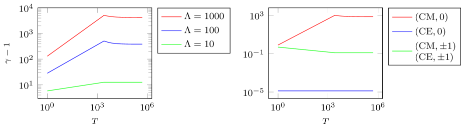
Figure 3: Specific kinetic energy transfer $\gamma-1$ to any charged test particle. On the left, the (CM,$1$) pulse has parameters $\{\Psi_{1}=1,\Psi_{2}=1000,\Phi=0.001,\Xi=1\}$. On the right, relative values of $\gamma-1$ are displayed for various $(s,\kappa)$ pulses with parameters $\{\Lambda=1,\Psi_{1}=1,\Psi_{2}=1000,\Phi=0.001,\Xi=1\}$. The differences between the energy transfers for some pulses appear indistinguishable relative to others owing to the logarithmic scales employed. In all cases, the charged particle has initial position $\{R(0)=1,\theta(0)=\frac{\pi}{2},Z(0)=1\}$ and initial velocity $\{\dot{R}(0)=0,\dot{Z}(0)=\frac{1}{200},\dot{\theta}(0)=0\}$.

The instantaneous specific relativistic kinetic energy of a particle with laboratory speed $v$ is $\gamma-1$ in terms of the Lorentz factor $\gamma$ given by $\gamma^{-1}=\sqrt{1-\frac{v^{2}}{c^{2}}}$. In figure 3, this quantity is displayed as a function of $T$ on the left for a charged particle accelerated by a fixed chirality (CM,$-1$) type pulse where the pulse energy is varied by changing $\Lambda$. On the right the energy transfer dependence on pulse chirality for both CE and CM type pulses with fixed laser energy is displayed. We deduce that the pulse momentum and angular momentum [26] in the propagation direction can transfer an impulsive force and torque respectively to charges lying in an orthogonal plane. More generally, the classical configurations of a high energy pulse labelled CE or CM could be distinguished experimentally by their interaction with different arrangements of charged matter.

Furthermore, by a suitable choice of parameters, (CE, $\kappa$) type modes can be constructed that yield the same physical properties ($\mathcal{J},z_{rg},z_{w},\beta$) for all $\kappa$. Similarly the (CM,$\kappa$) type modes yield a $\kappa$ independent set with physical properties distinct from those determined by the (CE,$\kappa$) modes. The pulse group speed magnitudes (as defined above) of all these configurations are determined numerically and are bounded above by the value $c$. To illustrate some of these statements, Table 1 summarizes the SI laser pulse characteristics determined by solving the system of equations in (6) for a specific choice of $\{\Psi_{1},\Psi_{2},\Phi,\Xi\}\,$ and various values of $\Lambda$, selected to demonstrate the physical characteristics of existing laser pulses. We conclude that both the CE and CM type pulses can propagate localized packets with linear and angular momentum analogous to the quantum characteristics of propagating wave packets describing particles with different masses.

These observations suggest that, for electromagnetic micropulses with ${\cal{E}}t_{0}\lesssim\hbar$, a parameterized effective quantum Hamiltonian $H$ describing a particular pair of interacting massive point particles may provide the simplest effective description of general non-stationary quantum states of a laser pulse. Such states are then defined as elements of a complex Hilbert space ${\cal H}=L^{2}(\mathbb{R}^{3},\mathbb{C}^{3})\otimes L^{2}(\mathbb{R}^{3},\mathbb{C}^{3})$ where each factor denotes the space of complex square integrable 3-component vectors on $\mathbb{R}^{3}$ carrying irreducible finite dimensional representations of the 3-dimensional rotation group. Such a construction is analogous to the Hilbert space ${\cal H}_{\text{vib}}\otimes{\cal H}_{\text{rot}}$ used in Bohm and Loewe’s dynamic model of a vibrating and rotating diatomic molecule after removing its translational degrees of freedom [27]. The space ${\cal H}_{\text{vib}}$ is spanned by eigenstates of the Hamiltonian $H_{\text{vib}}$ for a one-dimensional simple harmonic oscillator parameterized by a fundamental frequency $\omega_{0}$ and the space ${\cal H}_{\text{rot}}$ is spanned by eigenstates of the Hamiltonian $H_{\text{rot}}$ for a one-dimensional rigid rotator parameterized by a constant moment of inertia parameter $\cal{I}$. The simplest model for the diatomic molecule takes for its Hamiltonian:

$$H_{\text{mol}} = H_{\text{vib}}\otimes I+I\otimes H_{\text{rot }}+{\cal G}W_{\text{vib}}\otimes W_{\text{rot}}$$

in terms of the three phenomenological real parameters $\omega_{0},{\cal{I,G}}$ and where $I$ denotes the identity operator on the relevant space. For certain diatomic molecules this idealized model (and its refinements) accounts for well-established empirical formulae for their electronic energy states. States in the space ${\cal H}$ must describe the translational modes of a quantum packet as well as possible mode-mixing. To this end we model their unitary evolution generated by an effective Hermitian Hamiltonian of the form:

$$H = H_{\text{0}}({\mathbf{x}_{1}},{\mathbf{x}_{2}})+H_{\text{int}}({\mathbf{x}_{1}},{\mathbf{x}_{2}})$$

where

$$H_{\text{0}} = \left(-\frac{\hbar^{2}}{2\mu_{1}}\nabla^{2}_{\mathbf{x}_{1}}\right)\otimes I+I\otimes\left(-\frac{\hbar^{2}}{2\mu_{2}}\nabla^{2}_{\mathbf{x}_{2}}\right)$$

with real parameters $\mu_{1},\mu_{2}>0$. For quantum pulses that are deemed relativistic, one can include relativistic corrections by the replacement

$$-\frac{\hbar^{2}}{2\mu_{n}}\nabla^{2}_{\mathbf{x}_{n}}\quad\longrightarrow\quad\sqrt{-\hbar^{2}c^{2}\nabla^{2}_{\mathbf{x}_{n}}+\mu_{n}^{2}c^{4}\;}-\mu_{n}c^{2}$$

for $n=1,2$ and working in a momentum representation. The structure of $H_{\text{int}}({\mathbf{x}_{1}},{\mathbf{x}_{2}})$ depends upon the physical properties of the medium through which the pulse propagates. A simple model that accommodates quantum birefringence, medium anisotropy and inhomogeneity may be constructed in terms of parameterized Hermitian operators ${W}_{1}(\mathbf{x}_{1}),\,{W}_{2}(\mathbf{x}_{2})$:

$$H_{\text{int}} = {W}_{1}(\mathbf{x}_{1})\otimes{W}_{2}(\mathbf{x}_{2}).$$

The six classical chiral states labelled $(s,\kappa)$ that evolve according to the classical Maxwell equations are now replaced by elements $\Psi_{t}\in{\cal H}$ satisfying the Schrödinger equation:

$$-\frac{\hbar}{i}\frac{\partial}{\partial t}\Psi_{t} = H\Psi_{t}$$

with $\Psi_{t_{0}}$ prescribed at any time $t_{0}$ and satisfying $\langle\Psi_{t_{0}},\Psi_{t_{0}}\rangle=1$. In a direct product matrix representation, decomposable states in ${\cal H}$ can be written ${\boldsymbol{\alpha}}(t,{\mathbf{x}}_{1})\otimes{\boldsymbol{\beta}}(t,{\mathbf{x}}_{2})$ with

$${\boldsymbol{\alpha}}(t,{\mathbf{x}}_{1}) = \left(\!\begin{array}[]{c}{\alpha_{1}}(t,{\mathbf{x}}_{1})\\ {\alpha_{2}}(t,{\mathbf{x}}_{1})\\ {\alpha_{3}}(t,{\mathbf{x}}_{1})\end{array}\!\right)\qquad\text{and}\qquad{\boldsymbol{\beta}}(t,{\mathbf{x}}_{2})\;=\;\left(\!\begin{array}[]{c}{\beta_{1}}(t,{\mathbf{x}}_{2})\\ {\beta_{2}}(t,{\mathbf{x}}_{2})\\ {\beta_{3}}(t,{\mathbf{x}}_{2})\end{array}\!\right).$$

By analogy with the description of non-relativistic spin$-\frac{1}{2}$ qubit states, call ${\boldsymbol{\alpha}}$ the left qutrit component of such a bi-qutrit state and ${\boldsymbol{\beta}}$ the corresponding right qutrit component. The dynamic description of a general state $\psi_{t}\in{\cal H}$ requires an explicit interaction Hamiltonian operator. To model interactions with a classical medium we envisage here a smooth fabricated meta-material with specified inhomogeneous and anisotropic characteristics. This is similar to the specification of the magnetic moment interaction of the qubit states (due to an unpaired bound s-wave electron) of a silver atom with a classical (inhomogeneous) static magnetic field in the Stern-Gerlach experimental arrangement. An important practical distinction however arises since the laser states, unlike electrons, are electrically and magnetically neutral and hence their interaction with electromagnetically neutral properties of a fabricated meta-material may be more versatile than in the Stern-Gerlach situation [28].

Consider, for example, the evolution of the left qutrit component ${\boldsymbol{\alpha}}(t,{\mathbf{x}}_{1})$ under the Hamiltonian:

$$-\frac{\hbar^{2}}{2\mu_{1}}\nabla^{2}_{\mathbf{x}_{1}}\otimes I+G_{1}{\boldsymbol{S}}\cdot{\boldsymbol{N}}(t,{\mathbf{x}}_{1})\otimes I$$

where the constant $(3\times 3)$ Hermitian matrix-valued vector ${\boldsymbol{S}}$ satisfies the commutation relation ${\boldsymbol{S}}\times{\boldsymbol{S}}=i{\boldsymbol{S}},\,$ the 3-vector ${\boldsymbol{N}}(t,{\mathbf{x}}_{1})$ is a classical field of unit-vectors on some fabricated meta-material and $G_{1}$ is a parameter with the physical dimensions of energy. Such a Hamiltonian assigns a single preferred field of spatial directions ${\boldsymbol{N}}(t,{\mathbf{x}}_{1})$ for the interaction of quantum states with the medium. More complex media could involve multiple anisotropies described by a multi-directional set of unit-vector fields.

Given ${\boldsymbol{\alpha}}(0,{\mathbf{x}_{1}})$ with

$$\sum_{j=1}^{3}\int_{V}|\alpha_{j}(0,{\mathbf{x}_{1}})|^{2}\,d^{3}{\mathbf{x}_{1}} = 1$$

(assuming an unbounded medium $V$), one solves the system:

$$-\frac{\hbar}{i}\frac{\partial{\boldsymbol{\alpha}}(t,{\mathbf{x}}_{1})}{\partial t} = -\frac{\hbar^{2}}{2\mu_{1}}\nabla^{2}_{\mathbf{x}_{1}}{\boldsymbol{\alpha}}(t,{\mathbf{x}}_{1})+G_{1}\,{\boldsymbol{S}}\cdot{\boldsymbol{N}}(t,{\mathbf{x}}_{1})\,{\boldsymbol{\alpha}}(t,{\mathbf{x}}_{1})$$

for the left qutrit component at $t>0$. Multi-component wave-packet solutions can be constructed by the standard Fourier transform methods used to construct wave-packets for scalar fields. Thus in cylindrical polar coordinates $(r,\phi,z)$ defined with respect to a preferred time-independent, fixed $z-$direction ${\boldsymbol{N}}=(0,0,1)$ in a uniformly homogeneous medium, wave-packet solutions to the above equation take the form:

$$\alpha_{j}(t,r,\phi,z) = \!\!\sum_{m=-\infty}^{\infty}\int_{-\infty}^{\infty}\!\!dk\,A_{j,m}(k,s)\,\int_{0}^{\infty}\!\!\sqrt{sr}\,ds\,J_{m}(rs)\,\exp[ikz+im\phi]\;\Gamma_{j}(t,k,s)$$

for $j=1,2,3$ where

$$\Gamma_{1}(t,k,s) = \exp\left[\frac{it}{\hbar}\left(\frac{\hbar^{2}}{2\mu_{1}}(k^{2}+s^{2})+G_{1}\right)\right]$$

$$\Gamma_{2}(t,k,s) = \exp\left[\frac{it}{\hbar}\left(\frac{\hbar^{2}}{2\mu_{1}}(k^{2}+s^{2})\right)\right]$$

$$\Gamma_{3}(t,k,s) = \exp\left[\frac{it}{\hbar}\left(\frac{\hbar^{2}}{2\mu_{1}}(k^{2}+s^{2})-G_{1}\right)\right].$$

and the amplitudes $A_{j,m}(k,s)$ are determined from the normalised initial conditions $\alpha_{j}(0,r,\phi,z)$ by Fourier and Fourier-Bessel inversion. In these expressions contributions to $\alpha_{j}$ from terms in the sums that depend on the integer $m$ indicate those from eigenstates of the orbital angular momentum operator $\frac{\hbar}{i}{\mathcal{L}}_{\partial_{\phi}}$ [29]. By contrast, terms in ${\boldsymbol{\alpha}}$ with different $j$ refer to spin (qutrit) contributions to $\psi_{t}$. With the above Hamiltonian, stationary qutrit energy eigenstates would be non-degenerate with energy shifts $(0,\pm G_{1})$. Generating superpositions involving left and right qutrit states in ${\cal H}$ that cannot be reduced to decomposable states by a change of basis may offer a means to isolate and thereby control non-stationary entangled qutrits using appropriately fabricated meta-materials.

In addition to such laser state “measurement” interactions with a classical medium, one may also include interactions with atomic quantum states. These and other uses of such effective quantum Hamiltonians involving the dynamics of laser states will be discussed elsewhere.

4 Conclusions

We have constructed a basis of classical chiral solutions of the source-free vacuum Maxwell field equations from a simple particular solution to the complex scalar wave equation in spacetime and a set of covariantly constant antisymmetric tensor fields. Such solutions offer a simple 3-parameter description of a finite-energy laser pulse that provide a more accurate simulation tool for analysing laser-matter interactions in realistic 3-dimensional situations where plane-fronted paraxial approximations are inadequate. The analytic structure of such solutions enables one to readily extract all the standard diffractive characteristics associated with a laser pulse in free space. Using the classical relativistic Lorentz-force equation of motion we have also analysed numerically the interaction of such compact pulse solutions with charged point particles. This has explicitly demonstrated how laser configurations with definite chirality and mode-type transfer angular momentum and energy to the charges as a result of the interaction. From these numerical investigations we have proposed a particular effective quantum model for systems where the classical pulse energy ${\cal{E}}$ and the pulse duration $t_{0}$ satisfy ${\cal{E}}t_{0}\lesssim\hbar$. By analogy with the effective modelling of rotating-vibrating diatomic molecules we have proposed a simple phenomenological Hamiltonian that may be used to describe quantum laser packets in free space and material media. It is suggested that this Hamiltonian may have utility for simulating a novel transfer of quantum information and for constructing models of rapid single-cycle laser pulses interacting with quantum matter and classical fabricated materials containing structures below the nano-scale.

References

- [1] T. Brabec and F. Krausz. Intense few-cycle laser fields: Frontiers of nonlinear optics. Rev. Mod. Phys., 72(2):545, 2000.
- [2] S. Yoffe, Y. Kravets, A. Noble, and D. Jaroszynski. Longitudinal and transverse cooling of relativistic electron beams in intense laser pulses. New J. Phys., 17(5):053025, 2015.
- [3] A. Buck, M. Nicolai, K. Schmid, C. M. S. Sears, A. Sävert, J. M. Mikhailova, F. Krausz, M. C. Kaluza, and L. Veisz. Real-time observation of laser-driven electron acceleration. Nature Phys., 7(7):543–548, 2011.
- [4] N. H. Matlis, S. Reed, S. S. Bulanov, V. Chvykov, G. Kalintchenko, T. Matsuoka, P. Rousseau, V. Yanovsky, A. Maksimchuk, S. Kalmykov, G. Shvets, and M. C. Downer. Snapshots of laser wakefields. Nature Phys., 2(11):749–753, 2006.
- [5] F. Mackenroth, A. DiPiazza, and C. H. Keitel. Determining the carrier-envelope phase of intense few-cycle laser pulses. Phys. Rev. Letts., 105(6):063903, 2010.
- [6] F. S. Tsung, C. Ren, L. O. Silva, W. B. Mori, and T. Katsouleas. Generation of ultra-intense single-cycle laser pulses by using photon deceleration. Proc. Nat. Acad. Sci., 99(1):29–32, 2002.
- [7] R. W. Ziolkowski and M. K. Tippett. Collective effect in an electron plasma system catalyzed by a localized electromagnetic wave. Phys. Rev. A, 43(6):3066, 1991.
- [8] R. W. Ziolkowski. Metamaterial-based source and scattering enhancements: from microwave to optical frequencies. Opt-Elec. Rev., 14(3):167–177, 2006.
- [9] J-L Liu, Z-M Sheng, and J. Zheng. Exact solution of the vectorial field structure of a light beam. Opt. Comms., 284(19):4646–4649, 2011.
- [10] C. Harvey, T. Heinzl, and M. Marklund. Symmetry breaking from radiation reaction in ultra-intense laser fields. Phys. Rev. D, 84(11):116005, 2011.
- [11] F. Terranova. Particle acceleration in subcycle optical cells. Phys. Rev. ST Accel. Beams, 17:071301, 2014.
- [12] T. A. Raybould, V. A. Fedotov, N. Papasimakis, I. J. Youngs, and N. I. Zheludev. Focused electromagnetic doughnut pulses and their interaction with interfaces and nanostructures. arXiv:1512.04285, 2015.
- [13] A. B. Klimov, R. Guzman, J. C. Retamal, and C. Saavedra. Qutrit quantum computer with trapped ions. Phys. Rev. A, 67(6):062313, 2003.
- [14] R. W. Ziolkowski, J. M. Arnold, and D. M. Gogny. Ultrafast pulse interactions with two-level atoms. Phys. Rev. A, 52(4):3082, 1995.
- [15] R. W. Ziolkowski. Exact solutions of the wave equation with complex source locations. J. Math. Phys., 26(4):861–863, 1985.
- [16] R. W. Ziolkowski. Localized transmission of electromagnetic energy. Phys. Rev. A, 39(4):2005, 1989.
- [17] A. M. Shaarawi, I. M. Besieris, and R. W. Ziolkowski. Localized energy pulse trains launched from an open, semi-infinite, circular waveguide. J. Appl. Phys., 65(2):805–813, 1989.
- [18] R. Donnelly and R. Ziolkowski. A method for constructing solutions of homogeneous partial differential equations: localized waves. Proc. R. Soc. A: Math Phys. Sci., 437(1901):673–692, 1992.
- [19] R. Donnelly and R. W. Ziolkowski. Designing localized waves. Proc. R. Soc. A: Math Phys. Sci., 440(1910):541–565, 1993.
- [20] J. N. Brittingham. Focus waves modes in homogeneous Maxwell’s equations: Transverse electric mode. J. Appl. Phys., 54(3):1179–1189, 1983.
- [21] J. L. Synge. Relativity: the Special Theory. North-Holland Publishing Company, Amsterdam, 1956.
- [22] A. M. Fedotov, K. Y. Korolev, and M. V. Legkov. Exact analytical expression for the electromagnetic field in a focused laser beam or pulse. In The International Conference on Coherent and Nonlinear Optics, pages 672613–672613. International Society for Optics and Photonics, 2007.
- [23] S. Feng, H. G. Winful, and R. W. Hellwarth. Spatiotemporal evolution of focused single-cycle electromagnetic pulses. Phys. Rev. E, 59(4):4630, 1999.
- [24] G. N. Borzdov. Designing localized electromagnetic fields in a source-free space. Phys. Rev. E, 65(6):066612, 2002.
- [25] H. E. Hernández-Figueroa, M. Zamboni-Rached, and E. Recami. Localized Waves, volume 194. 2007.
- [26] L. Allen, S. M. Barnett, and M. J. Padgett. Optical Angular Momentum. CRC Press, 2003.
- [27] A. Bohm and M. Loewe. Quantum Mechanics: Foundations and Applications, volume 3. Springer New York, 1986.
- [28] N. F. Mott. The scattering of fast electrons by atomic nuclei. Proc. Roy. Soc. A: Math. Phys., 124(794):425–442, 1929.
- [29] O. Matula, A. G. Hayrapetyan, V. G. Serbo, A. Surzhykov, and S. Fritzsche. Atomic ionization of hydrogen-like ions by twisted photons: angular distribution of emitted electrons. J. Phys. B: At. Mol. Opt. Phys., 46(20):205002, 2013.