Probability distribution functions of gas in M31 and M51

Abstract

We present probability distribution functions (PDFs) of the surface densities of ionized and neutral gas in the nearby spiral galaxies M31 and M51, as well as of dust emission and extinction $A_{V}$ in M31. The PDFs are close to lognormal and those for $\mathrm{H\,\scriptstyle I}$ and $A_{V}$ in M31 are nearly identical. However, the PDFs for $\mathrm{H}_{2}$ are wider than the $\mathrm{H\,\scriptstyle I}$ PDFs and the M51 PDFs have larger dispersions than those for M31. We use a simple model to determine how the PDFs are changed by variations in the line-of-sight (LOS) pathlength $L$ through the gas, telescope resolution and the volume filling factor of the gas, $f_{v}$. In each of these cases the dispersion $\sigma$ of the lognormal PDF depends on the variable with a negative power law. We also derive PDFs of mean LOS volume densities of gas components in M31 and M51. Combining these with the volume density PDFs for different components of the ISM in the Milky Way (MW), we find that $\sigma$ decreases with increasing length $L$ with an exponent of $-0.76\pm 0.06$, which is steeper than expected. We show that the difference is due to variations in $f_{v}$. As $f_{v}$ is similar in M31, M51 and the MW, the density structure in the gas in these galaxies must be similar. Finally, we demonstrate that an increase in $f_{v}$ with increasing distance to the Galactic plane explains the decrease in $\sigma$ with latitude of the PDFs of emission measure and FUV emission observed for the MW.

1 Introduction

Many processes can leave an imprint on the complicated structure of the interstellar medium (ISM) observed in the Milky Way and nearby galaxies. For example, variations in the gas density can be due to: an evolving population of gravitationally bound clouds; expanding supernova remnant shells compressing the gas; cooling and heating of the gas leading to phase transitions; the turbulent and compressible nature of the flow.

During the last two decades compressible turbulence has been recognized as an important cause of the density structure of the ISM in the Milky Way. Both isothermal (Elmegreen & Scalo, 2004, and references therein) and multi-phase (de Avillez & Breitschwerdt, 2005; Wada & Norman, 2007) simulations of the ISM produced lognormal volume density distributions. Several authors noted that for a large enough volume and for a long enough simulation run, the physical processes causing the density fluctuations in the ISM in a galactic disc can be regarded as random, independent, multiplicative events (e.g. Vázquez-Semadeni, 1994; Passot & Vázquez-Semadeni, 1998; Wada & Norman, 2007). Therefore, the PDF of log(density) becomes Gaussian and the density PDF lognormal, as long as the local Mach number and the density are not correlated (Kritsuk et al., 2007; Federrath et al., 2010). However, Tassis et al. (2010) show that lognormal column density distributions in molecular clouds are a generic statistical representation of the inhomogeneous distribution of gas density, whether the inhomogeneity is a result of turbulence, gravity or ambipolar diffusion. Recent reviews which discuss density PDFs of molecular clouds and their connection to turbulence and star formation include McKee & Ostriker (2007); Hennebelle & Falgarone (2012); Padoan et al. (2013) and recent theoretical modelling can be found in Federrath, Klessen & Schmidt (2008); Federrath (2013); Federrath & Klessen (2013).

Observational evidence to test the simulation results is slowly growing. Padoan et al. (1997), Goodman, Pineda & Schnee (2009), Kainulainen et al. (2009), Schmalzl et al. (2010), Schneider et al. (2012) and Kainulainen et al. (2014) obtained lognormal column density PDFs for the extinction through dust in molecular clouds in the Milky Way (MW). The latter authors discuss the relationship between the density PDFs and star formation. Schneider et al. (2013) presented lognormal PDFs of 12CO(1-0) integrated intensities for four dust clouds in the MW, and Hughes et al. (2013) found lognormal PDFs of the 12CO(1-0) brightness temperature and integrated intensities in M51. Also the PDF of the $\mathrm{H}_{2}$ column densities in M33 is lognormal, but with a high-density tail (Druard et al., 2014). Wada, Spaans & Kim (2000) showed that the luminosity function of the $\mathrm{H\,\scriptstyle I}$ column density in the Large Magellanic Cloud is lognormal. Hill et al. (2007, 2008) found lognormal distributions of the emission measures, which are proportional to the integral of the electron density squared, in the Wisconsin $\mathrm{H}\alpha$ Mapper survey (Haffner et al., 2003) perpendicular to the Galactic plane at latitudes $|b|>10^{\circ}$, and along the plane, with different parameters. The emission measures of the extinction-corrected $\mathrm{H}\alpha$ emission from the galaxy M33 (Tabatabaei et al., 2007) and the volume density of the dust-bearing gas near stars within $400\,\mathrm{pc}$ from the Sun (Gaustad & Van Buren, 1993) have lognormal distributions. Furthermore, Seon (2011, 2013) obtained lognormal PDFs for the FUV background emission from the ISRF, and Bowen et al. (2008) plotted the volume density distribution of the $\mathrm{O\,\scriptstyle VI}$-line emitting gas in the MW, which is approximately lognormal. Recently, Berkhuijsen & Fletcher (2008, 2012) showed that in the Milky Way the volume density distribution of the diffuse, ionized gas (DIG) at $|b|>5^{\circ}$, and of the diffuse atomic gas are close to lognormal. They also discussed differences in the PDF dispersion observed for the atomic gas at low and high latitudes, and of warm and cold gas. Here we present the PDFs of ionized and neutral gas column densities in the nearby galaxies M31 and M51, which are close to lognormal, and discuss their properties.

Unfortunately, we cannot separate the variation in gas density due to turbulence from variations caused by e.g. supernova explosions, HII regions or gravitation. Therefore, our PDFs capture all kinds of density structure along the lines of sight (LOS), regardless of the origin. On the other hand, high-density structures represent only a small fraction of the volume of the radio beams at our spatial resolution of about 300 $\mathrm{pc}$. We will interpret the properties of the observed PDFs in terms of an effective LOS, $L_{\mathrm{eff}}$, which is the fraction of the total LOS occupied by turbulent cells and gas clouds. Furthermore, purely for the sake of clarity in the text, we will refer only to clouds rather than to clouds or turbulent cells. In reality, we cannot make a firm distinction. We shall return to this point at the end of the paper.

The paper is organized as follows: The data sets used are described in Section 2, and we show the derived PDFs and discuss their properties in Section 3. Simple models to examine the effects of varying resolution, line-of-sight path length and the gas filling factor on the form of the PDFs are presented in Section 4. We compare the observed properties of the PDFs to those expected from simulation studies in Section 5, and in Section 6 we summarize our results.

2 The data

M31, the spiral galaxy nearest to us, is at a distance of $780\pm 40\,\mathrm{kpc}$ (Stanek & Garnavich, 1998). The Sb galaxy of large angular extent (more than $3^{\circ}\times 1^{\circ}$) and low surface brightness has an inclination of $i=77.5^{\circ}$ (Braun, 1991; Chemin, Carignan & Foster, 2009) and so is nearly edge-on. The position angle is $PA=37.7^{\circ}$ . Our gas density PDFs are based on the Westerbork $\mathrm{H\,\scriptstyle I}$ survey of Brinks & Shane (1984) at an angular resolution of $24\times 36\,\rm{arcsec^{2}}$, corrected for missing spacings, the IRAM 12CO(1-0) survey of Nieten et al. (2006) at a resolution of 23 arcsec, and the extinction corrected $\mathrm{H}\alpha$ data of Devereux et al. (1994), at a resolution of a few arcsec, produced by Tabatabaei & Berkhuijsen (2010). Nieten et al. (2006) converted the CO data to column densities of molecular gas using the constant conversion factor $X_{\mathrm{CO}}=1.9\times 10^{20}\,\mathrm{mol}\,\mathrm{cm}^{-2}\,(\mathrm{K}\,\mathrm{km}\,\mathrm{s}^{-1})^{-1}$. Before deriving the PDF we smoothed each map to an angular resolution of 45 arcsec, corresponding to $170\,\mathrm{pc}\times 785\,\mathrm{pc}$ along major $\times$ minor axis in the plane of M31. Each PDF was calculated from independent data points (at least $1.67\times$ beamwidth apart) above $2\times$ rms noise.

M51 is a bright Sbc galaxy at a distance of 7.6 Mpc (Ciardullo et al., 2002). It has an angular extent of about 10 arcmin, a position angle of $PA=-10^{\circ}$  and an inclination of $i=20^{\circ}$ (Tully, 1974; Pety et al., 2013). For the PDFs we used the $\mathrm{H\,\scriptstyle I}$ data from the THINGS survey (Walter et al., 2008) at a resolution of $5.82\times 5.56\,\rm{arcsec^{2}}$, the BIMA 12CO(1-0) survey of Helfer et al. (2003) at a resolution of $5.8\times 5.1\,\rm{arcsec^{2}}$, which was corrected for missing spacings using single-dish observations, and the $\mathrm{H}\alpha$ map of Greenawalt et al. (1998) at a resolution of a few arcsec. All maps were reduced to a common field of about $8.5\times 10.5\,\rm{arcmin^{2}}$ covering most of M51 apart from the extended southern outer arm in $\mathrm{H\,\scriptstyle I}$. They were then smoothed to a resolution of 8 arcsec corresponding to $295\times 315\,\mathrm{pc}^{2}$ along major $\times$ minor axis in the plane of M51. We converted the CO data to column densities of $\mathrm{H}_{2}$ using the conversion factor $4.75\times 10^{19}\,\mathrm{mol}\,\mathrm{cm}^{-2}\,(\mathrm{K}\,\mathrm{km}\,\mathrm{s}^{-1})^{-1}$, one quarter of that for the Milky Way (Guelin et al., 1995). Of each map, only independent data points above $2\times$ rms noise were used to produce the PDF.

3 Probability distribution functions

In this Section we present the observed surface density PDFs for M31 and M51 and characterise them by fitting lognormal distributions to the histograms. Since there are various ways to paramaterise a lognormal we shall briefly describe the exact equations we use. To allow for easy comparison with Berkhuijsen & Fletcher (2008) and other work on observed PDFs we use common, or base 10, logarithms. The lognormal probability distribution function for the random variable $x$ is given by

$$\Lambda(x|\mu,\sigma)=\frac{\log_{\mathrm{10}}e}{\sigma x\sqrt{2\pi}}\exp{[-(\log_{\mathrm{10}}{x}-\mu)^{2}/2\sigma^{2}]}\,\mathrm{d}x,$$ (1)

which is equivalent to a Gaussian distribution for $\log_{\mathrm{10}}(x)$,

$$N[\log_{\mathrm{10}}(x)|\mu,\sigma]=\\ \frac{1}{\sigma\sqrt{2\pi}}\exp{[-(\log_{\mathrm{10}}{x}-\mu)^{2}/2\sigma^{2}]}\,\mathrm{d}\log_{\mathrm{10}}x.$$ (2)

We use Eq. 2 to derive $\mu$ and $\sigma$ from fits to histograms of $\log_{\mathrm{10}}(x)$, taking into account the logarithmic bin-width to ensure that the integral of the PDF is unity. It is important to note that $\mu$ and $\sigma$ are the mean and standard deviation of the Gaussian distribution of $\log_{\mathrm{10}}(x)$; the mean and standard deviation of the distribution of $x$ are given by

$$E[x]=\exp{(\mu+\sigma^{2}/2)},$$

and

$$S[x]=\sqrt{(\exp{\sigma^{2}}-1)\exp{(2\mu+\sigma^{2})}},$$

respectively. Thus the variance of $x$ depends on both the mean and standard deviation of $\log_{\mathrm{10}}(x)$. We shall try to avoid confusion by calling $\sigma$ the dispersion of the PDF and using $X_{0}=10^{\mu}$ to describe the peak of the PDF (note that $10^{\mu}$ is the median of the distributions of both $x$ and $\log_{\mathrm{10}}(x)$). For the Gaussian PDFs of $\log_{\mathrm{10}}(x)$, which is the form we show in our figures, small (large) values of $\sigma$ result in a narrow (broad) Gaussian PDF.

3.1 PDFs of surface densities

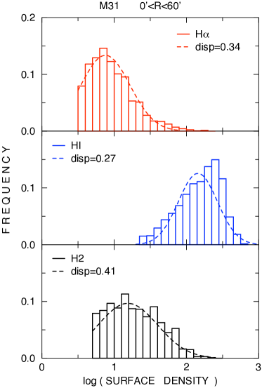
Figure 1: Probability distribution functions of the surface densities of ionized and neutral gas in the radial interval $0\arcmin<R<60\arcmin$ in M31. Top: $\mathrm{H}\alpha$ (in $\mathrm{cm}^{-6}\,\mathrm{pc}$), middle: $N(\mathrm{H\,\scriptstyle I})$ (in $10^{19}\,\mathrm{atom}\,\mathrm{cm}^{-2}$), bottom: $N(\mathrm{H}_{2}$) (in $10^{19}\,\mathrm{mol}\,\mathrm{cm}^{-2}$). Dashed lines show the lognormal fits given in Table 1.

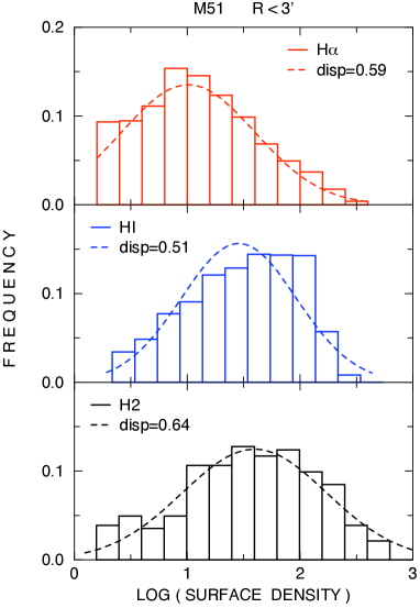
Figure 2: Probability distribution functions of the surface densities of ionized and neutral gas in M51. Top: $\mathrm{H}\alpha$ (in $\mathrm{cm}^{-6}\,\mathrm{pc}$), middle: $N(\mathrm{H\,\scriptstyle I})$ (in $10^{19}\,\mathrm{atom}\,\mathrm{cm}^{-2}$), bottom: $N(\mathrm{H}_{2}$) (in $10^{19}\,\mathrm{mol}\,\mathrm{cm}^{-2}$). Dashed lines show the lognormal fits given in Table 2.

In Fig. 1 we present the M31 PDFs of the emission measures of the ionized gas and of the column densities of $\mathrm{H\,\scriptstyle I}$ and $\mathrm{H}_{2}$ for the radial range $0\arcmin<R<60\arcmin$ in the plane of the galaxy, corresponding to $0<R<13.6\,\mathrm{kpc}$. In Table 1 we list the parameters of the lognormal fits together with those for the area containing the bright emission ring ($35\arcmin<R<60\arcmin$ or $7.9<R<13.6\,\mathrm{kpc}$) and for the weaker emission interior to this ’ring’ ($0\arcmin<R<35\arcmin$). For $\mathrm{H}\alpha$ and $\mathrm{H}_{2}$ the fits of the PDFs for the subregions are nearly the same, but for $\mathrm{H\,\scriptstyle I}$ the position of the peak of the PDF, $X_{0}$, for the bright ’ring’ is at a significantly higher density than for the inner region and the dispersion is smaller. This difference in $X_{0}$ causes the low-density excess — and hence the asymmetry — in the total PDF and its larger dispersion compared to that of the subregions.

Figure 2 shows the M51 PDFs of the emission measures of the ionized gas and of the column densities of $\mathrm{H\,\scriptstyle I}$ and $\mathrm{H}_{2}$ at radii $R<3\arcmin$. The parameters of the lognormal fits are given in Table 2. Again the $\mathrm{H\,\scriptstyle I}$ PDF has an excess at low densities. The peak at high densities is due to gas in the outer spiral arms. We have tried to construct separate PDFs for spiral arms and the interarm regions by using a spiral-arm mask; this was created using the coefficients of a wavelet transform of the CO map with a scale of about $1\,\mathrm{kpc}$, the positive coefficients tracing a clear two-armed spiral. Although the dispersions of these PDFs could not be reliably determined, the values of $X_{0}$ of the arm PDFs are significantly higher than of the PDFs for the interarm regions. Recently, Hughes et al. (2013) found that PDFs of the integrated 12CO(1-0) intensities in M51 for arm regions are clearly wider than for interarm regions, and have an about 25 per cent larger $X_{0}$. They also presented PDFs for the inner $4.5\arcmin\times 2.8\arcmin$ of M51. At a spatial resolution of $53\,\mathrm{pc}$, using all pixels with an intensity above 3 times the noise, they obtained a dispersion of $\sigma=0.62$, the same as our value for a larger area of M51 observed at a lower resolution.

Table 1: Lognormal fits to the PDFs of gas surface densities in M31, HPBW $45\arcsec$.

				Position of maximum		Dispersion
$X$	Units	$R(\arcmin)$	$N$	$\mu$	$X_{0}$	$\sigma$	$\chi^{2}$
$N(\mathrm{H\,\scriptstyle I})$	$10^{19}\,\mathrm{atom}\,\mathrm{cm}^{-2}$	0–60	1249	$2.16\pm 0.03$	$145\pm 10$	$0.27\pm 0.02$	12.7
		0–35	368	$1.86\pm 0.01$	$72\pm 2$	$0.23\pm 0.01$	0.8
		35–60	881	$2.32\pm 0.02$	$209\pm 10$	$0.19\pm 0.01$	5.5
$N(\mathrm{H}_{2}$)	$10^{19}\,\mathrm{mol}\,\mathrm{cm}^{-2}$	0–60	971	$1.19\pm 0.04$	$15.5\pm 1.5$	$0.41\pm 0.02$	2.9
		0–35	250	$1.11\pm 0.05$	$12.9\pm 1.6$	$0.39\pm 0.04$	1.5
		35–60	721	$1.22\pm 0.04$	$16.6\pm 1.6$	$0.40\pm 0.03$	3.0
$\mathrm{H}\alpha$	$\mathrm{cm}^{-6}\,\mathrm{pc}$	0–60	1097	$0.88\pm 0.03$	$7.6\pm 0.5$	$0.34\pm 0.02$	2.9
		0–35	397	$0.93\pm 0.03$	$8.5\pm 0.6$	$0.34\pm 0.02$	1.2
		35–60	700	$0.85\pm 0.03$	$7.1\pm 0.5$	$0.34\pm 0.02$	2.3

N is the total number of data points; the error in each bin $\delta_{i}$ is estimated as $\delta_{i}=\sqrt{N_{i}}$ for (number of bins$-2$) degrees of freedom; $\chi^{2}$ is the reduced chi-squared goodness of fit parameter.

Table 2: Lognormal fits to the PDFs of gas surface densities in M51 at $R<3\arcmin$, HPBW $8\arcsec$.

			Position of maximum		Dispersion
$X$	Units	$N$	$\mu$	$X_{0}$	$\sigma$	$\chi^{2}$
$N(\mathrm{H\,\scriptstyle I})$	$10^{19}\,\mathrm{atom}\,\mathrm{cm}^{-2}$	2015	$1.46\pm 0.05$	$28.7\pm 3.3$	$0.51\pm 0.05$	6.4
$N(\mathrm{H}_{2}$)	$10^{19}\,\mathrm{mol}\,\mathrm{cm}^{-2}$	282	$1.60\pm 0.05$	$39.4\pm 4.5$	$0.64\pm 0.05$	1.1
$\mathrm{H}\alpha$	$\mathrm{cm}^{-6}\,\mathrm{pc}$	728	$1.01\pm 0.04$	$10.2\pm 1.0$	$0.59\pm 0.03$	1.4

N is the total number of data points; the error in each bin $\delta_{i}$ is estimated as $\delta_{i}=\sqrt{N_{i}}$ for (number of bins$-2$) degrees of freedom; $\chi^{2}$ is the reduced chi-squared goodness of fit parameter.

The PDFs of $\mathrm{H}\alpha$, $\mathrm{H\,\scriptstyle I}$ and $\mathrm{H}_{2}$ for M31 and M51 presented in Figs. 1 and 2 are close to lognormal. That the PDFs of $\mathrm{H}_{2}$ are lognormal may seem surprising in view of the recent work of Shetty et al. (2011). In their simulations of molecular clouds, the authors found that the PDFs of 12CO(1-0)-intensities and of CO column densities are generally not lognormal and have different shapes when CO is optically thick. But at low densities and for the model of a Milky Way cloud of medium density the PDFs are lognormal. The box size in their simulations is $20\,\mathrm{pc}$, much smaller than the typical resolution of $300\,\mathrm{pc}$ used for the PDFs of the gas surface densities in M31 and M51. Hence, the line intensity seen by the radio beam is the average intensity of a large sample of individual clouds. Saturated lines will hardly be observed because the filling factor of the densest clouds is very small. Therefore the observed CO PDFs become lognormal and will give a fair representation of the PDF of the $\mathrm{H}_{2}$ column density.

Comparing Figures 1 and 2 we note the following:

(a) Both PDFs of $\mathrm{H}\alpha$ show a low-intensity cut-off at the sensitivity limit. A similar cut-off occurs in the PDF of $\mathrm{H}_{2}$ for M31.

(b) The $\mathrm{H}\alpha$ PDF for M51 extends to higher emission measures than that for M31 and the emission measure of the maximum is about 35% higher than that of M31. Since the M51 data were not corrected for extinction and the inclination of M51 is smaller than that of M31, this means that the face-on surface brightness in $\mathrm{H}\alpha$ of M51 is much larger than that of M31.

(c) The steep decrease seen in the $\mathrm{H\,\scriptstyle I}$ PDFs at high column densities may be attributed to opacity in the $\mathrm{H\,\scriptstyle I}$ lines. In scatter plots of star-formation rate against $\mathrm{H\,\scriptstyle I}$ mass surface density a cut-off near $10\,\mathrm{M}_{\odot}\,\mathrm{pc}^{-2}$ is visible in M31 (Tabatabaei & Berkhuijsen, 2010), M51 and many other galaxies (Bigiel et al., 2008). Braun et al. (2009) have shown that after correcting the HI column densities of M31 for opacity the apparent cut-off vanishes.

(d) The $\mathrm{H\,\scriptstyle I}$ column densities of M31 extend to higher values than those of M51 and the maximum of the PDF of M31 occurs at a column density that is 5 times that of M51. On the sky, M31 is much brighter in $\mathrm{H\,\scriptstyle I}$ than M51, but the face-on value of $X_{0}$, defined as $X_{0}\cos{i}$, of M31 is only about 1.2 times that of M51. The $\mathrm{H\,\scriptstyle I}$ PDF for M51 has a pronounced low-density tail, while that for M31 only shows a mild low-density excess. The low-density tail of the M51 PDF may be a relic of the last encounter with the companion galaxy NGC5195 (Howard & Byrd, 1990) that gave rise to the extended $\mathrm{H\,\scriptstyle I}$ arm in the south-east (Rots et al., 1990).

(e) The $\mathrm{H}_{2}$ column densities of M51 are much higher than of M31: the face-on value of $X_{0}$ of M51 is 11 times that of M31. The star formation rate of M51 is five times higher than that of M31 (Tabatabaei et al., 2013), which may be related to the higher column densities reached in M51 than in M31 (Kainulainen et al., 2014). $\mathrm{H}_{2}$ is the dominant gas phase in the inner part of M51 (García-Burillo et al., 1993; Schuster et al., 2007), while in M31 the atomic gas is the dominant component (Dame et al., 1993; Nieten et al., 2006).

3.2 PDFs of volume densities in M31

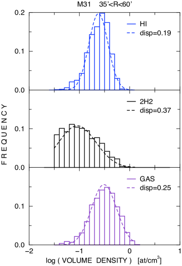
Figure 3: Probability distribution functions of mean volume densities along the line of sight (in $\mathrm{cm^{-3}}$) of neutral gas in the radial interval $35\arcmin<R<60\arcmin$, the bright emission ’ring’, in M31. Top: $\langle n_{\mathrm{H\,\scriptstyle I}}\rangle$, middle: $\langle 2n_{\mathrm{H}}2\rangle$, bottom: $\langle n\rangle=\langle n_{\mathrm{H\,\scriptstyle I}}\rangle+\langle 2n_{\mathrm{H}}2\rangle$. Dashed lines show the lognormal fits given in Table 3.

Table 3: Lognormal fits to the PDFs of gas volume densities in M31, HPBW $45\arcsec$.

				Position of maximum		Dispersion
$X$	Units	$R(\arcmin)$	$N$	$\mu$	$X_{0}$	$\sigma$	$\chi^{2}$
$\langle n_{\mathrm{H\,\scriptstyle I}}\rangle$	$\mathrm{atom}\,\mathrm{cm}^{-3}$	0–60	1457	$-0.75\pm 0.03$	$0.178\pm 0.012$	$0.25\pm 0.02$	12.5
		0–35	459	$-1.00\pm 0.02$	$0.100\pm 0.005$	$0.23\pm 0.01$	1.6
		35–60	998	$-0.62\pm 0.02$	$0.240\pm 0.011$	$0.19\pm 0.01$	5.7
$\langle n_{2\mathrm{H}_{2}}\rangle$	$\mathrm{atom}\,\mathrm{cm}^{-3}$	0–60	920	$-1.05\pm 0.03$	$0.089\pm 0.006$	$0.39\pm 0.02$	2.6
		0–35	248	$-1.08\pm 0.05$	$0.083\pm 0.010$	$0.41\pm 0.03$	1.3
		35–60	672	$-1.04\pm 0.03$	$0.091\pm 0.007$	$0.37\pm 0.02$	2.0
$\langle n\rangle$	$\mathrm{atom}\,\mathrm{cm}^{-3}$	0–60	1451	$-0.61\pm 0.02$	$0.245\pm 0.012$	$0.30\pm 0.01$	5.1
		0–35	457	$-0.82\pm 0.02$	$0.151\pm 0.007$	$0.32\pm 0.01$	1.1
		35–60	994	$-0.51\pm 0.01$	$0.309\pm 0.007$	$0.25\pm 0.01$	2.6

$\chi^{2}$ is the reduced chi-squared goodness of fit parameter: the error in each bin $\delta_{i}$ is estimated as $\delta_{i}=\sqrt{N_{i}}$ for (number of bins$-2$) degrees of freedom.

We calculated the mean $\mathrm{H\,\scriptstyle I}$ volume densities, $\langle n_{\mathrm{H\,\scriptstyle I}}\rangle$, from the column densities using the formula for the $\mathrm{H\,\scriptstyle I}$ scale height increasing with radius, $h(R)$, given by Braun (1991), scaled to the distance $D=780\,\mathrm{kpc}$. This gives $h(10\arcmin)=240\,\mathrm{pc}$ and $h(60\arcmin)=425\,\mathrm{pc}$. The volume density then is $\langle n_{\mathrm{H\,\scriptstyle I}}\rangle=N(\mathrm{H\,\scriptstyle I})/L$ where the line of sight $L=2h(R)/\cos{i}$. Assuming a scale height of the molecular gas equal to $h(R)/2$ yielded the mean volume densities of the molecular gas, $\langle n_{2\mathrm{H}_{2}}\rangle$. The volume density of all neutral gas then is $\langle n\rangle=\langle n_{\mathrm{H\,\scriptstyle I}}\rangle+\langle n_{2\mathrm{H}_{2}}\rangle$. As an example, we present the PDFs of these volume densities for the ’ring’ in Fig. 3 and the lognormal fits for all regions in Table 3. The $\mathrm{H\,\scriptstyle I}$ PDF is narrower and more symmetric than that for the full area shown in Fig. 1 because the low-density extension is not included. It is shifted by a factor of 2.4 w.r.t. the PDF for the inner region. Comparison with Table 1 shows that the dispersions of the PDFs of $\langle n_{\mathrm{H\,\scriptstyle I}}\rangle$ and $\langle n_{2\mathrm{H}_{2}}\rangle$ are the same as those of the column density PDFs within the errors (see Section 4 for a simple explanation for this equivalence.). These estimates for the mean volume density PDFs are useful in that they allow us to compare the properties of M31 with those of the Milky Way in Section 5.2.

4 Dependence of density PDF parameters on pathlength, resolution and filling factor

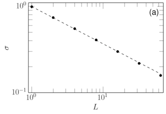
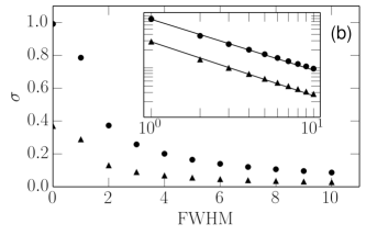
Figure 4: (a) The effect of an increasing LOS on the dispersion ($\sigma$ in Eq. (1)) of the best fit lognormal PDF. The dashed line shows the best-fit power-law. (b) The effect of smoothing with a 2D Gaussian, of unit mean and full-width half-maximum shown on the horizontal axis, on $\sigma$. Circles are for models with $L=1$ and triangles for $L=10$. The inset panel shows the best-fit power-laws to the data points where $\mathrm{FWHM}\geq 1$. In both panels the modelled column densities were calculated using the simple model described in Section 4.

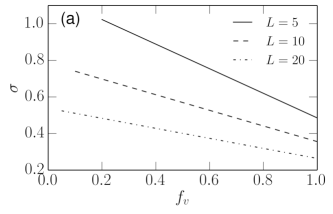
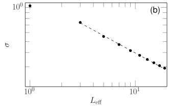
Figure 5: (a) The effect of varying fractional volume, $f_{v}$, on the dispersion ($\sigma$ in Eq. (1)) of the best fit lognormal PDF of the average volume density. Lines are shown for different LOS. (b) $\sigma$ versus the effective LOS $L_{\mathrm{eff}}$ as defined in the text. The best-fit power-law for $L_{\mathrm{eff}}>1$ is shown. In both panels the modelled average volume densities, the column density divided by the LOS, were calculated using the simple model described in Section 4.

The maps used to compute the column and average volume density histograms presented in Section 3 all have a resolution of a few hundred parsec. The presence of a lognormal density PDF does not in itself indicate that the gas is turbulent, the lognormal PDFs are merely compatible with this assumption (Tassis et al., 2010; Hennebelle & Falgarone, 2012). One could consider two contributions to the column density PDFs: one from the density structure arising from compressible turbulence in the ISM and the other from the densities of specific, discrete objects that are not caused by turbulence, such as SNRs and $\mathrm{H\,\scriptstyle II}$ regions (both of which may, however, be drivers of turbulence). How to separate these contributions to the PDF is not clear. Both types of structure have sizes less than the beam. The dominant energy input driving turbulence in the ISM is probably due to stellar cluster winds and superbubbles produced by clustered supernovae, with a typical scale in the range $50$–$500\,\mathrm{pc}$ (Elmegreen & Scalo, 2004, Section 3). Many other drivers of turbulence, such as spiral shocks, the magneto-rotational instability and proto-stellar jets have also been proposed (see Federrath & Klessen, 2013, for a discussion of these in the context of PDFs). The $\mathrm{H}_{2}$ at the largest scale is collected in giant molecular clouds (GMCs), with a typical size of $50\,\mathrm{pc}$ (Blitz et al., 2007) to $100\,pc$ in M51 (Colombo et al., 2014), and the $\mathrm{H}\alpha$ has a diffuse component as well as higher density $\mathrm{H\,\scriptstyle II}$ regions of typical size $30\,\mathrm{pc}$ (Habing & Israel, 1979; Scoville et al., 2001; Azimlu, Marcinak & Barmby, 2011). The thickness of the diffuse gas layer is of the order of $500\,\mathrm{pc}$ and that of the $\mathrm{H}_{2}$ $150\,\mathrm{pc}$, so each telescope-beam cylinder will contain one or many turbulent cells or GMCs or $\mathrm{H\,\scriptstyle II}$ regions. Furthermore, the ISM consists of several phases, so the emission that we use to construct the average volume density PDFs is not uniformly distributed along the total LOS but only arises from a fraction of this distance. In order to understand how averaging over multiple cells or clouds, both along and across the beam, and how the filling factor of the ISM occupied by the phase we observe affect the density PDFs we constructed a simple model.

4.1 A simple model for the random gas density distribution in the ISM

Independent random numbers drawn from a lognormal distribution with parameters $\mu=0$, $\sigma=1$ — see Eqs. (1) and (2) — were distributed over a Cartesian $(x,y,z)$ grid of $(1000\times 1000\times L)$ mesh-points. The value of each mesh-point represents the gas density of a single gas cloud and the unit of distance in the model is thus the cloud size. The parameter $L$ represents the line-of-sight and for $L>1$ the random numbers were summed along the $z$-axis to give a map of the column density of the model, with $1000\times 1000$ lines of sight. An average volume density along each line of sight was also computed by dividing the column density by $L$. Convolution of the column density with a 2D Gaussian of a given full-width half-maximum (FWHM) was used to model the consequences of smoothing by a beam of size $D=\mathrm{FWHM}$.

Making ($1-f_{v}$) of the mesh-points empty allowed us to control the fractional volume occupied by the clouds, $f_{v}=V/(1000\times 1000\times L)$, where $V$ is the number of meshpoints for which the gas density is non-zero. The empty mesh-points were chosen at random. We shall refer to $f_{v}$ as the volume filling factor but stress that there are at least two other quantities that are also called filling factors. Both measure the “clumpiness” of a given gas phase, either averaged over the entire volume or only the volume occupied by that phase, and calculated using the ratio $\langle n\rangle^{2}/\langle n^{2}\rangle$ where $n$ is the gas density and $\langle\dots\rangle$ represents the appropriate average: note that the relation between these filling factors and $f_{v}$ is not straightforward (see Gent et al., 2013, Sect. 5). Under the assumption that the gas is confined to clouds which all have the same density, which is commonly made when deriving filling factors from observational data (see e.g. Berkhuijsen & Fletcher, 2008), the fractional volume occupied by the gas and the volume filling factor defined as $\langle n\rangle^{2}/\langle n^{2}\rangle$ are the same. We adopt this assumption in what follows; in other words we assume that the fractional volume and the volume filling factor are one and the same quantity.

Normalised histograms of the column or average-volume density gave the model PDFs, and the best-fitting lognormal function to the PDF, using a least-squares method, was used to compute $\mu$ and $\sigma$ for each model. Ten independent realisations were calculated for each set of model parameters and the resulting $\mu$ and $\sigma$ averaged. For $L=1$, $f_{v}=1$, and perfect resolution (no smoothing), the model PDFs have the same parameters, $\mu=0$ and $\sigma=1$, as the lognormal distribution used to populate the model (within a numerical error due to the finite size of the mesh and the constraints of the fitting algorithm). We used the model to explore how $\sigma$, as this is by far the most useful of the two parameters in interpreting observations, varies as $L$, $f_{v}$ and $D$ change.

4.2 PDF dispersion and the pathlength

Figure 4(a) shows how the dispersion of the lognormal PDF, $\sigma$, changes as the pathlength along the line of sight, $L$, is increased. Here $f_{v}=1$ and no smoothing is applied. For $L=1$ the model recovers $\sigma=1$, as required by the parameters of the original distribution of densities. As $L$ increases $\sigma$ decreases as a power law $\sigma\propto L^{\alpha}$. The fitted power law in Fig.  4(a) has $\alpha=-0.4$ for the range $1<L<64$, but as the lower end of the range in $L$ increases (i.e. for $L\gg 1$) we find that $\alpha\rightarrow-0.5$. This scaling is in agreement with Fischera & Dopita (2004) who studied the relationship between $\sigma$ of the column density PDF and the ratio of $L$ to the size of a turbulent cell, $L/s_{\mathrm{max}}$: for thick discs, i.e. $L/s_{\mathrm{max}}\gg 1$, they derived $\sigma\propto(L/s_{\mathrm{max}})^{-0.5}$. In our simple models $s_{\mathrm{max}}=1$ and so $L/s_{\mathrm{max}}\geq 1$.

4.3 PDFs of column and average volume densities

The scaling of $\sigma$ with $L$ for the lognormal PDFs of the average volume density, defined as $\langle n\rangle=\Sigma/L$, follows the same power law behaviour as the column density PDFs: for $n$ we also find that $\sigma\propto L^{-0.5}$ for $L\gg 1$. This is not surprising, as dividing a lognormal by a constant changes $\mu$ but not $\sigma$ (e.g. Aitchison & Brown, 1957, Theorem 2.1). In these models we set $f_{v}=1$ and applied no smoothing.

4.4 PDF dispersion and beam smoothing

Figure 4(b) shows how $\sigma$ changes under smoothing of the model column (and volume) densities, where we have fixed $f_{v}=1$. Smoothing reduces $\sigma$ and for beamwidths $D\geq 1$ the scaling follows a power law, shown in the inset to the Figure, with $\sigma\propto D^{-1}$ irrespective of $L$. This power law behaviour means that when $D\gtrsim 4$-$5$ clouds for shallow $L$ and $D\gtrsim 2$-$3$ clouds for longer $L$, the effect on $\sigma$ of further moderate smoothing is marginal: the resolution of observations of nearby galaxies is typically in the range $1<D<10$. In principle, if observations are available with a resolution of $D<s_{\mathrm{max}}$ and repeated smoothing results in $\sigma\propto D^{-1}$ beyond a certain beamwidth, one could recover $s_{\mathrm{max}}$ from the column density PDFs.

4.5 PDF dispersion and the filling factor

Figure 5(a) shows that as the filling factor increases, i.e. as the gas occupies more of the total volume, the dispersion of the fitted lognormal PDFs for the average volume density decreases linearly. However, the effect on $\sigma$ depends on both $L$ and $f_{v}$. If $f_{v}$ is a constant for all lines of sight, then the power law scaling $\sigma\propto L^{{\alpha}}$ with $\alpha=-0.5$ still holds. However, if $f_{v}$ depends on $L$ this scaling can change. This motivates us to define the effective pathlength

$$L_{\mathrm{eff}}=f_{v}L$$ (3)

which is the fraction of the total line of sight that is occupied by clouds or turbulent cells. Figure 5 shows that $\sigma$ scales as a power law $\sigma\propto L_{\mathrm{eff}}^{\alpha}$ for $L_{\mathrm{eff}}>1$. The best fit power law has an index $\alpha=-0.5$, as in the models where $f_{v}=1$ shown in Fig. 4(a).

4.6 Summary of model results

For convenience we summarise the results obtained using this simple model for a lognormal distribution of gas density in the ISM. We shall use these results to interpret the observations.

1. The dispersions of the lognormal column density and average volume density PDFs both scale as a power law with the total line of sight, $\sigma\propto L^{\alpha}$. When the filling factor $f_{v}=1$ both have $\alpha=-0.5$.

2. Smoothing by the telescope beam, when the beam is bigger than the size of a cloud, results in a power law scaling $\sigma\propto D^{-1}$. For $D\gtrsim 5s_{\mathrm{max}}$ in a thin layer ($L/s_{\mathrm{max}}\sim 1$) and $D\gtrsim 2s_{\mathrm{max}}$ in a thicker layer ($L/s_{\mathrm{max}}\sim 10$), further smoothing only produces a weak effect on $\sigma$.

3. $\sigma$ is linearly related to the filling factor of the gas but the magnitude of the effect also depends on $L$. Defining the effective pathlength $L_{\mathrm{eff}}=f_{v}L$ results in the scaling $\sigma\propto L_{\mathrm{eff}}^{-0.5}$.

5 Discussion

Two differences between the PDFs shown in Figs.  1–3 and Tables  1–3 are immediately obvious: the M51 PDFs are significantly wider than the M31 PDFs and for both galaxies the $\mathrm{H}_{2}$ PDF is wider than the $\mathrm{H\,\scriptstyle I}$ PDF. Which factors could cause these differences?

Simulations of the ISM have shown that the dispersion of a PDF depends on variables like disk mass, temperature, magnetic field strength, length of the line of sight and density scale. Furthermore, we showed in Section 4 that also the filling factor plays a role. Below we consider each of these factors separately.

The width of the PDF increases with the gas density in the disc (Tassis, 2007; Wada & Norman, 2007). In the HD simulations of Wada & Norman (2007) an increase of a factor of 10 in disc mass leads to an increase in the dispersion of 30%. As the mean face-on column density of the total gas in M51 is about 5 times higher than that in M31 (calculated from the $\mathrm{H\,\scriptstyle I}$ and $\mathrm{H}_{2}$ PDFs with $\langle N\rangle=X_{0}\exp(\sigma_{\ln}^{2}/2)$ and added (Ostriker et al., 2001)), this could account for a difference of about 15 per cent in the dispersions of the gas PDFs for the two galaxies.

In the MHD simulations of de Avillez & Breitschwerdt (2005), the dispersion of the PDF of cold gas is wider than that of warm or hot gas. This was confirmed by the HD simulations of Robertson & Kravtsov (2008) and Gent et al. (2013). Since the molecular gas is generally cooler than the atomic gas, the temperature difference could cause the $\mathrm{H}_{2}$ PDF to be wider than the $\mathrm{H\,\scriptstyle I}$ PDF. Unfortunately, we cannot estimate the expected difference in dispersion because the temperature ranges in the figures of these simulation papers are too large.

Molina et al. (2012) simulated the development of molecular clouds with time using a MHD code. They derived relations between the dispersion of the PDF, the Mach number $M$ and plasma $\beta$, the ratio between thermal and magnetic pressure. They found that increasing $M$, i.e.  more cooler and denser gas, widens the PDFs of the clouds (see also Federrath et al., 2008; Price et al., 2011; Federrath, 2013), consistent with our observations, whereas decreasing $\beta$ makes the PDFs somewhat narrower. We can estimate the ratio of mean $\beta$ in M51 to that in M31 by comparing the thermal and magnetic pressures in the two galaxies. As the total thermal pressure is dominated by the ionized gas, we use $X_{0}$ of the $\mathrm{H}\alpha$ PDFs (Tables 1 and 2) and the lines of sight $L$ given in Tables 4 and 5 to calculate the rms electron density $\sqrt{\langle n_{e}^{2}\rangle}$ for each galaxy. This is 2.9 times higher in M51 than in M31 suggesting that in M51 the thermal pressure is about three times higher than in M31. As the magnetic field in M51 (Fletcher et al., 2011) is about three times stronger than in M31 (Fletcher et al., 2004), the magnetic pressure in M51 is about nine times higher than in M31; hence, $\beta$ in M51 is about one third of that in M31. Molina et al. (2012) set $\beta\propto M^{-2}$ in their simulations of molecular clouds. If this relationship also holds in less dense gas phases, a three times smaller $\beta$ would imply a $\sqrt{3}=1.7$ times higher mean $M$ in M51 than in M31. Since $M$ affects the PDF dispersion more strongly than $\beta$ (see Molina et al., 2012), the PDFs for M51 will be wider than those for M31, in agreement with our observations. Separate measurements of $M$ and $\beta$ will be necessary to see how large this effect is compared to other influences on the width of the PDF.

The scale of the density fluctuations influences the dispersion of the PDF because an increase in the number of clouds seen by the radio beam leads to a decrease in the dispersion as extremes are averaged out (Ostriker et al., 2001; Vázquez-Semadeni & Garcia, 2001). In Section 4 we demonstrated that this effect may occur across the beam area as well as along the LOS. In Section 5.1 we show that the angular resolution hardly influences the observed dispersion, and in Section 5.2 that the effective length of the LOS is the dominant factor in shaping the observed PDFs.

5.1 Does the observed dispersion depend on beamwidth?

In Section 4 we showed that the dispersion $\sigma$ of the column density PDFs varies strongly under smoothing when the smoothing beamwidth is smaller than about $5$ clouds, but that once the beamwidth is larger than this the effect of further smoothing becomes negligible. Thus the behaviour of the best fit $\sigma$ under repeated smoothing can, in principle, be used to set a rough upper limit on the correlation size of the clouds.

Figure 6: Dependence of the dispersion $\sigma$ of the PDFs of the column densities $N(\mathrm{H\,\scriptstyle I})$ (dots) and $N(\mathrm{H}_{2}$) (triangles) on the half-power beamwidth (in arcseconds) for the radial interval $0\arcmin<R<60\arcmin$ in M31. A beamwidth of $45\arcsec$ corresponds to $170\,\mathrm{pc}\times 785\,\mathrm{pc}$ in the plane of the galaxy. The lines are weighted least-squares fits to the data points.

We investigated this point for the column densities of $\mathrm{H\,\scriptstyle I}$ and $\mathrm{H}_{2}$ of M31. To this end we smoothed the $\mathrm{H\,\scriptstyle I}$ and $\mathrm{H}_{2}$ maps with Gaussian functions to angular resolutions of 24 arcsec $\times$ 36 arcsec (indicated by 30 arcsec), 90 arcsec and 180 arcsec, and calculated the PDFs. Including the PDFs at 45 arcsec and the original resolution of 23 arcsec of the $\mathrm{H}_{2}$ map, the range spans a factor of 7.8 in scale. We found that for the full region $R<60\arcmin$ as well as for the subregions the dispersions of the PDFs are the same within the errors for both $\mathrm{H\,\scriptstyle I}$ and $\mathrm{H}_{2}$ (see Fig. 6). Hence, the dispersion of the gas PDFs for M31 is independent of smoothing scale between about $90\,\mathrm{pc}\times 400\,\mathrm{pc}$ and $700\,\mathrm{pc}\times 3150\,\mathrm{pc}$ in the plane of M31.

Since the LOS through the disc of M31 is large (on average $~{}3000\,\mathrm{pc}$ for the $\mathrm{H\,\scriptstyle I}$ disc), Fig. 4(b) suggests that smoothing will not affect $\sigma$ when the FWHM is wider than about 2 clouds. We can use this to make an estimate of the upper limit to the size of the clouds in M31. The smallest of the smoothing scales we consider, $90\,\mathrm{pc}\times 400\,\mathrm{pc}$, must contain at least $2^{2}=4$ clouds, giving an estimate for the upper limit of the size of the clouds of $s_{\mathrm{max}}<\sqrt{(400\times 90)/4}=95\,\mathrm{pc}$.

Note that the linear resolution of the M51 observations is about $300\,\mathrm{pc}$, similar to that of the best resolved $\mathrm{H\,\scriptstyle I}$ observations of M31. Therefore, the difference in dispersion of the PDFs of the gas surface densities for M31 and M51 cannot be caused by a difference in angular resolution, provided the scales of the clouds are the same.

5.2 Line-of-sight effects

In the case of column density PDFs, Figure 4(a) shows that at a fixed resolution the fitted $\sigma$ will be smaller by about a factor of $2$ for a $4$-times longer LOS. In particular, we found that $\sigma$ decreases with $L^{-0.5}$. We observe this effect in the PDFs of M31 and M51 in several ways.

First, the PDFs of M31 (Fig. 1) have a smaller dispersion than those of M51 (Fig. 2). The LOS through the strongly inclined galaxy M31 is typically about 4 times longer than the LOS through M51 that is nearly seen face-on, provided that the scale heights are similar. Assuming that the cloud scales in the two galaxies are comparable, we then expect more clouds along the LOS through M31 than along the LOS through M51, and hence smaller dispersions of the PDFs for M31 than for M51.

Second, for both M31 and M51 the PDFs of $\mathrm{H}_{2}$ are significantly wider than those of $\mathrm{H\,\scriptstyle I}$. Since the molecular gas is more concentrated in the disc mid-plane than $\mathrm{H\,\scriptstyle I}$ (due to the larger gravitational forces) and molecular clouds are generally denser and smaller than $\mathrm{H\,\scriptstyle I}$ clouds, the LOS through molecular gas are shorter than through $\mathrm{H\,\scriptstyle I}$ gas leading to a larger dispersion of the $\mathrm{H}_{2}$ PDF than of the $\mathrm{H\,\scriptstyle I}$ PDF. Also the Mach number of the $\mathrm{H}_{2}$ gas is higher than of the $\mathrm{H\,\scriptstyle I}$ gas (because the temperature is much lower whereas the turbulent velocity is similar), causing a higher compression of the gas in the molecular clouds by turbulent shocks and larger dispersions of the cloud PDFs (Molina et al. (2012) and references therein). However, this effect may be reduced if the LOS intersects many clouds, or if the beamwidth is larger than the typical cloud size: in this case the peak of the PDF may move to a higher density but the dispersion can be unchanged. Which of these two effects is responsible for the observed difference in the PDF dispersions requires further study.

Third, the $\mathrm{H\,\scriptstyle I}$ PDF for the inner region of M31 is slightly wider ($\sigma=0.23\pm 0.01$) than that for the bright ’ring’ ($\sigma=0.19\pm 0.01$) where the LOS is longer and goes through more clouds than in the inner region. This interpretation is supported by the higher value of $X_{0}$ in the ’ring’. The same trend is visible in the $\mathrm{H}_{2}$ PDFs (see Table 3).

Furthermore, the dispersions of gas PDFs derived in numerical simulations of the ISM (e.g. Vázquez-Semadeni & Garcia, 2001; de Avillez & Breitschwerdt, 2005; Wada & Norman, 2007) are usually larger than observed PDFs. Berkhuijsen & Fletcher (2008) attributed the difference to the higher densities used in the simulations compared to observed densities. However, the much smaller lines of sight available in simulations than in observations may be the main cause of the larger dispersions of PDFs derived from simulations (see also Fischera & Dopita, 2004).

It is possible to quantify the relationship between the dispersion of column density PDFs and LOS. Because the scale height of the gas in M31 increases outwards, we can test this relationship using the PDFs of the average volume densities of the sub-regions at different radii given in Table 3.

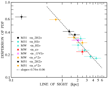
Figure 7: Dependence of the dispersion $\sigma$ of the PDFs of mean gas volume densities in M31, the Milky Way and M51 on line of sight $L$ (in pc). We assumed an uncertainty of $25\%$ in $L$. The dashed line is the weighted least-squares fit given by Eq. 4. (The figure is shown in colour in the electronic version of the paper.)

In Fig. 7 we show the dispersion of the PDFs of average volume density of $\mathrm{H\,\scriptstyle I}$ and 2$\mathrm{H}_{2}$ as function of the mean LOS $L$ of the radial ranges $0\arcmin<R<35\arcmin$ and $35\arcmin<R<60\arcmin$, where $L=2h(R)/\cos{i}$ and $h(R)$ is the scale height as derived in Section 3.2.

We have added 3 points for the mean volume density of diffuse $\mathrm{H\,\scriptstyle I}$ (cool and warm $\mathrm{H\,\scriptstyle I}$) towards stars in the solar neighbourhood (SN) and for the mean volume density of free electrons in the diffuse ionized gas (DIG) at Galactic latitudes $|b|>5^{\circ}$ within a few kpc from the sun as well as two points of mean electron density squared obtained from emission measures towards pulsars, all taken from Berkhuijsen & Fletcher (2008, 2012). We also show the dispersion of the $\mathrm{O\,\scriptstyle VI}$ PDF calculated along the lines of sight to 190 stars using fig. 9 (left panels) in Bowen et al. (2008).

For M51 scale heights of molecular and ionized gas are available. Pety et al. (2013) combined CO surveys observed with Plateau de Bure and the 30-m IRAM telescope. An extensive analysis showed that the molecular gas not only has a thin disc with a Gaussian scale height of $h=40\,\mathrm{pc}$, but also a thick disc with a scale height of about 250 $\mathrm{pc}$. Taking the about 8 times higher volume density of the thin disc in the mid-plane into account, their sum can be desribed by a single exponential with a scale height of about 75 $\mathrm{pc}$. Seon (2009) modelled the $\mathrm{H}\alpha$ emission from M51 observed by Thilker, Braun & Walterbos (2000) and derived a thin disc of $\mathrm{H\,\scriptstyle II}$- regions with exponential scale height of 300 $\mathrm{pc}$  and a thick disc of DIG with 1 $\mathrm{kpc}$  scale height. In the mid-plane the emission from the thin disc is about 7 times stronger than that from the DIG. The sum of the two distributions can be approximated by a single exponential disc with a scale height of 350 $\mathrm{pc}$. We have added the dispersions of $N(\mathrm{H}_{2}$) and $\mathrm{H}\alpha$ given in Table 2 using the single scale heights obtained above for the LOS $L$. Details on the data points in Fig. 7 are given in Table 4.

Apart from the $N(\mathrm{H}_{2}$)-point of M51 (that we discuss below), the dispersions in Fig. 7 systematically decrease with increasing $L$. A weighted fit through the 12 available points yields the power law

$$\log[\sigma(L)]=(2.0\pm 1.7)-(0.76\pm 0.06)\log[L]$$ (4)

with $\chi^{2}=0.3$ and $L$ in pc.

We conclude that the length of the line of sight through the gas in M31, the MW and M51 is the main influence on the width of the PDFs of average volume density. This implies that the number of clouds along the LOS determines the dispersion of the PDF.

Since the data points for the Milky Way and $\mathrm{H}\alpha$ for M51 in Fig. 7 are consistent with the M31 points, the variation in cloud sizes must be similar in these galaxies. This conclusion is supported by the work of Azimlu, Marcinak & Barmby (2011), who found that the size distributions of $\mathrm{H\,\scriptstyle II}$ regions in different galaxies are very similar, but the total number of $\mathrm{H\,\scriptstyle II}$ regions differs depending on the star formation rate.

We note that most of the data points in Fig. 7 forming the $\sigma$ - $L$ relation refer to diffuse gas. Much of the $\mathrm{H\,\scriptstyle I}$ in M31 is known to be diffuse (Braun & Walterbos, 1992) and the small amount of molecular gas in M31 may ’look’ diffuse in our large radio beam because it does not contain many small, dense $\mathrm{H}_{2}$ clouds.

Table 4: Effective lines of sight $L_{\mathrm{eff}}$ and filling factors

Gal.	Gas	Zone	N	L	$L_{\mathrm{eff}}$ [pc]	$f_{v}$	Dispersion	Ref.
M31	$2\mathrm{H}_{2}$	$R<35\arcmin$	248	1370	$60\pm 15$	$0.04\pm 0.02$	$0.41\pm 0.03$	1
		$R>35\arcmin$	672	1770	$70\pm 15$	$0.04\pm 0.01$	$0.37\pm 0.02$	1
	$\mathrm{H\,\scriptstyle I}$	$R<35\arcmin$	459	2730	$180\pm 40$	$0.07\pm 0.02$	$0.23\pm 0.01$	1
		$R>35\arcmin$	998	3560	$270\pm 60$	$0.08\pm 0.02$	$0.19\pm 0.01$	1
MW	$\mathrm{H\,\scriptstyle I}_{c}$	$|b|>5^{\circ}$	64	2050	$130\pm 40$	$0.06\pm 0.03$	$0.27\pm 0.03$	3
	$\mathrm{H\,\scriptstyle I}_{w}$	$|b|>5^{\circ}$	98	2300	$90\pm 25$	$0.04\pm 0.01$	$0.33\pm 0.03$	2
		$|b|<5^{\circ}$	42	4630	$300\pm 65$	$0.06\pm 0.02$	$0.18\pm 0.01$	2
	$N_{e}$	$|b|>5^{\circ}$	34	2480	$200\pm 50^{*}$	$0.08\pm 0.02$	$0.22\pm 0.02^{*}$	2
	$\mathrm{O\,\scriptstyle VI}$	$|z|>200\mathrm{pc}$	190	2040	$100\pm 25$	$0.05\pm 0.02$	$0.31\pm 0.02$	4
	$N_{e}^{2}$	$|b|>5^{\circ}$	34	2480	$115\pm 25$	$0.05\pm 0.02$	$0.29\pm 0.02$	2
			157	1700	$85\pm 20$	$0.05\pm 0.02$	$0.34\pm 0.03$	2
M51	$\mathrm{H}_{2}$	$R<3\arcmin$	282	160	$24\pm 6$	$0.15\pm 0.05$	$0.64\pm 0.05$	1
	$\mathrm{H}\alpha$		728	750	$28\pm 6$	$0.04\pm 0.01$	$0.59\pm 0.03$	5

N=number of LOS; assumed errors in L: 25%, ^∗ $\sigma=0.22\pm 0.02$ and $L_{\mathrm{eff}}=200\pm 50\,\mathrm{pc}$ calibrate $L_{\mathrm{eff}}$ (see text). References: 1. This work; 2. Berkhuijsen & Fletcher (2008); 3. Berkhuijsen & Fletcher (2012); 4. Obtained from data in Bowen et al. (2008); 5. Seon (2009).

5.3 Importance of volume filling factor

The power-law dependence of $\sigma$ on $L$ presented in Fig. 7 has an exponent of $-0.76\pm 0.06$, which is $-0.26$ smaller than expected from the models in Sect. 4. However, the density structure in the ISM contains holes and voids in and between gas clouds (e.g. Elmegreen, 1997, 1998; de Avillez & Breitschwerdt, 2005) and so we should also take into account the volume filling factor, $f_{v}$, of the gas using Eq. (3).

Estimates of $f_{v}$ from observations (Dickey, 1993; Berkhuijsen, 1999) and simulations (de Avillez & Breitschwerdt, 2005; Gent et al., 2013) have shown that $\mathrm{H\,\scriptstyle I}$ gas has a larger filling factor than the denser molecular gas. So in Fig. 7 $f_{v}$ will increase with increasing $L$ and $L_{\mathrm{eff}}$ will increase faster than $L$.

For the $\langle n_{e}\rangle$-point for the MW at $L=2480\,\mathrm{pc}$ in Fig. 7, Berkhuijsen & Müller (2008) derived a volume filling factor of $f_{v}=0.08\pm 0.02$. Hence the effective LOS producing the dispersion of $0.22\pm 0.02$ is $L_{\mathrm{eff}}=(0.08\pm 0.02)*2480\approx 200\pm 50\,\mathrm{pc}$. Assuming that the relation $\sigma\propto L_{\mathrm{eff}}^{-0.5}$ found in Sect. 4 holds in the ISM, we can estimate $L_{\mathrm{eff}}$  for the other points in Fig. 7 using the observed $\sigma$ in $\sigma/(0.22\pm 0.02)=(L_{\mathrm{eff}}/(200\pm 50))^{-0.5}$. The volume filling factor then is $f_{v}=L_{\mathrm{eff}}/L$.

We list the observed and derived properties of the 13 points in Fig. 7 in Table 4. The errors given are random errors only. The error of 25 per cent in $L_{\mathrm{eff}}$  of the calibration point is systematic and affects all $L_{\mathrm{eff}}$  and $f_{v}$ in the same way. As expected, the values of $L_{\mathrm{eff}}$  increase with increasing $L$ varying between about $25\,\mathrm{pc}$ in M51 and more than $200\,\mathrm{pc}$ in the nearly edge-on galaxy M31. The filling factors, though, vary much less: in M31 between $0.04\pm 0.01$ for $\mathrm{H}_{2}$  and $0.08\pm 0.02$ for the $\mathrm{H\,\scriptstyle I}$ point at $L=3560\,\mathrm{pc}$. Apart from the deviating $\mathrm{H}_{2}$ point for M51, also the other filling factors are in this range. These values seem amazingly small, but they compare well with other information. For the cold ($\mathrm{H}_{2}$ and HI) gas at temperatures $T<200\mathrm{K}$, Breitschwerdt & de Avillez (2005) found from their MHD simulations $f_{v}=0.06$. Gent et al. (2013) derived from their simulations $f_{v}=0.03$ for cold gas at temperatures $T<500\mathrm{K}$. In their OVI-line study, Bowen et al. (2008) estimate that the size of the gas regions causing these lines is about 100-200$̇\mathrm{pc}$. Since the mean distance is $L=2040\,\mathrm{pc}$, $f_{v}=0.049-0.098$ for these regions, consistent with our value of $f_{v}=0.05\pm 0.02$. We note that at $L=2480\,\mathrm{pc}$ $\sigma$ of $<n_{e}^{2}>$ is larger than $\sigma$ of $<n_{e}>$, as one would expect. The larger $\sigma$ of $<n_{e}^{2}>$ leads to values of $L_{\mathrm{eff}}$  and $f_{v}$ that are nearly half of those of $<n_{e}>$, in agreement with the smaller scale height and larger clumpiness of HII regions compared to the DIG.

In Fig. 7 the $\mathrm{H}_{2}$ point for M51 is located at a much smaller LOS than is expected from the relation formed by the other 12 data points. This may be due to the large filling factor of $f_{v}=0.15\pm 0.05$, which is three to four times larger than $f_{v}$ of the $\mathrm{H}_{2}$ points for M31 (see Table 4). In the inner parts of M51 ($R<3\arcmin$) the dominant gas component is $\mathrm{H}_{2}$  (e.g. Pety et al., 2013)), while in M31 $\mathrm{H\,\scriptstyle I}$ is the dominant component (e.g. Nieten et al., 2006). At the end of Sect. 3.1 we showed that the mean face-on column density of $\mathrm{H}_{2}$ in M51 is 11 times higher than that of M31, which explains the higher value of $f_{v}$ in M51. When the filling factor is high, already a small effective LOS contains so many clouds that the PDF becomes lognormal. As $L_{\mathrm{eff}}$  in M51 is only about $25\,\mathrm{pc}$, the maximum size of the clouds along the LOS must be much less than $25\,\mathrm{pc}$.

Since the dispersion of the column density PDF is the same as that of the PDF of the average volume density (see Sect. 4), we can estimate $L$ of $\mathrm{H}\alpha$ in M31 and of $\mathrm{H\,\scriptstyle I}$ in M51 from Eq. 4 using the observed dispersions. This yields $L=1750\pm 1500\,\mathrm{pc}$ for $\mathrm{H}\alpha$ in M31, similar to that of $\mathrm{H}_{2}$ at $R>35\arcmin$. Using the same scaling for $L_{\mathrm{eff}}$  as above, we find $L_{\mathrm{eff}}=85\pm 20\,\mathrm{pc}$ and $f_{v}=0.05\pm 0.02$ (see Table 5). The value of $L$ implies a scale height of $190\pm 160\,\mathrm{pc}$, the same as for the $\mathrm{H}_{2}$ in the emission ring. This scale height of $\mathrm{H}\alpha$ is consistent with the observation of Walterbos & Braun (1994) that the z-extent of the DIG in M31 is less than about 500 $\mathrm{pc}$. If Eq. 4 and the scaling for $L_{\mathrm{eff}}$ also hold for the $\mathrm{H\,\scriptstyle I}$ gas in M51, then the observed dispersion in Table 2 indicates a LOS of about $1\,\mathrm{kpc}$ (see Table  5). The corresponding $L_{\mathrm{eff}}$  and filling factor of $L_{\mathrm{eff}}=37\pm 10\,\mathrm{pc}$ and $f_{v}=0.04\pm 0.01$, respectively, are smaller than in M31, which may be due to the small $\mathrm{H\,\scriptstyle I}$ content in M51.

Table 5: Estimates of LOS from dispersion of column density PDF.

Gal.	Comp.	L	$L_{\mathrm{eff}}$	$f_{v}$	Dispersion
		[pc]	[pc]
M31	$\mathrm{H}\alpha$	$1750\pm 1500$	$85\pm 20$	$0.05\pm 0.04$	$0.34\pm 0.02$
	$R<60\arcmin$
M51	$\mathrm{H\,\scriptstyle I}$	$1030\pm 900$	$37\pm 10$	$0.04\pm 0.03$	$0.51\pm 0.05$

Interestingly, Seon (2009) presented separate $\mathrm{H}\alpha$ PDFs for the DIG and the $\mathrm{H\,\scriptstyle II}$ regions in M51 based on the data of Thilker, Braun & Walterbos (2000). Although the scale heights differ by a factor of three (300 $\mathrm{pc}$  and 1000 $\mathrm{pc}$  for $\mathrm{H\,\scriptstyle II}$ regions and the DIG, repsectively), both PDFs have a dispersion of $0.36\pm 0.03$, but the position of their maxima differs by about a factor of 7. The LOS through the DIG would be $2130\,\mathrm{pc}$ and the dispersion of $0.36\pm 0.03$ is not far from the value of $0.29\pm 0.09$ expected from Eq.  4, but the point for the $\mathrm{H\,\scriptstyle II}$ regions PDF with an LOS of $640\,\mathrm{pc}\,$ disagrees with the value of $\sigma=0.73\pm 0.14$ expected from Eq.  (4). The same dispersion for the two layers indicates that $L_{\mathrm{eff}}$ is the same and the difference in LOS then means that the volume filling factors and/or the maximum cloud scales differ. Using the same scaling as before, we find that $\sigma=0.36\pm 0.03$ corresponds to $L_{\mathrm{eff}}=75\pm 20\,\mathrm{pc}\,$ giving $f_{v}=0.04\pm 0.01$ for the DIG and $f_{v}=0.12\pm 0.04$ for the disc of $\mathrm{H\,\scriptstyle II}$  regions. The filling factor of the $\mathrm{H\,\scriptstyle II}$ regions is similar to that of the $\mathrm{H}_{2}$ clouds in M51 suggesting that their density structure is similar.

It is worth noting that as the PDFs for the disc and the DIG in M51 are strongly shifted in $\log(X_{0})$, their combination yields a much wider PDF than that of the separate components. Thus our $\mathrm{H}\alpha$ PDF for M51 is not representative for small regions or specific components. This poses a general problem for the interpretation of PDFs for large regions in galaxies containing diffuse, low-density regions as well as dense spiral arms.

5.4 Estimating Mach numbers using PDFs: a note of caution

A connection between the dispersion of the density PDF $\sigma$ and the Mach number $\mathcal{M}$ of interstellar turbulence has been identified theoretically (e.g. Padoan et al., 1997; Passot & Vázquez-Semadeni, 1998; Ostriker et al., 2001; Federrath et al., 2008, 2010; Price et al., 2011; Molina et al., 2012) and used to make an estimate of $\mathcal{M}$ from observations (e.g. Padoan et al., 1997; Hill et al., 2008; Berkhuijsen & Fletcher, 2008). However, since the magnitude of $\sigma$ depends on the length of the LOS $L$, the telescope resolution $D$ and the volume filling factor of the gas $f_{v}$, caution should be exercised in applying the theoretical relation to real data. To make a reliable estimate of $\mathcal{M}$ one needs to know something about the distribution of the observed gas and so correct the observed $\sigma$ for the effects of $L$, $D$ and $f_{v}$.

5.5 M31: PDFs of dust emission and extinction

In view of the generally lognormal shapes of the gas PDFs, one may ask whether other constituents of the ISM also have lognormal PDFs. The dust emission is a good candidate since dust optical depth and gas column density are well correlated in the solar neighbourhood (Bohlin, Savage & Drake, 1978) and in M31 (Tabatabaei & Berkhuijsen, 2010), and lognormal PDFs of molecular gas column density and of extinction through dust clouds in the MW have been reported (e.g. Padoan et al., 1997; Goodman, Pineda & Schnee, 2009; Kainulainen et al., 2009; Schneider et al., 2013).

Table 6: Lognormal fits to the PDFs of dust emission from M31, HPBW $45\arcsec$. The fitted function is $Y=(\sqrt{2\pi}\sigma)^{-1}\exp[-(\log_{10}X-\mu)^{2}/2\sigma^{2}]$.

				Position of maximum		Dispersion
$X$	Units	$R(\arcmin)$	$N$	$\mu$	$X_{0}$	$\sigma$	$\chi^{2}$
$24\mu\mathrm{m}$	MJy/sr	0–60	1508	$-0.47\pm 0.01$	$0.34\pm 0.01$	$0.34\pm 0.01$	1.2
		0–35	525	$-0.48\pm 0.02$	$0.33\pm 0.01$	$0.33\pm 0.01$	1.4
		35–60	983	$-0.46\pm 0.01$	$0.35\pm 0.01$	$0.35\pm 0.01$	0.8
$70\mu\mathrm{m}$	MJy/sr	0–60	1426	$0.43\pm 0.02$	$2.69\pm 0.13$	$0.39\pm 0.01$	1.6
		0–35	502	$0.41\pm 0.03$	$2.57\pm 0.18$	$0.37\pm 0.02$	1.8
		35–60	924	$0.43\pm 0.02$	$2.69\pm 0.13$	$0.39\pm 0.01$	1.3
$160\mu\mathrm{m}$	MJy/sr	0–60	1516	$1.36\pm 0.01$	$23.4\pm 0.6$	$0.26\pm 0.01$	1.8
		0–35	535	$1.30\pm 0.01$	$20.0\pm 0.5$	$0.26\pm 0.01$	1.5
		35–60	981	$1.40\pm 0.01$	$25.1\pm 0.6$	$0.26\pm 0.01$	1.4
$A_{\mathrm{v}}$	mag.	0–60	1406	$-0.04\pm 0.02$	$0.91\pm 0.04$	$0.20\pm 0.01$	6.6
		0–35	495	$-0.16\pm 0.02$	$0.69\pm 0.03$	$0.25\pm 0.01$	1.9
		35–60	910	$0.01\pm 0.01$	$1.02\pm 0.03$	$0.18\pm 0.01$	4.4

$Y$ is the fraction of sightlines in each bin divided by the logarithmic bin- width $\mathrm{d}(\log_{10}X)$. $\chi^{2}$ is the reduced chi-squared goodness of fit parameter, with the error in each bin $\delta_{i}$ estimated as $\delta_{i}=\sqrt{N_{i}}$ and for (number of bins$-2$) degrees of freedom.

We calculated the PDFs of the dust emission from M31 at $24\,\mu\mathrm{m}$, $70\,\mu\mathrm{m}$ and $160\,\mu\mathrm{m}$ using the Spitzer MIPS maps of Gordon et al. (2006) smoothed to a resolution of 45 ″  by Tabatabaei & Berkhuijsen (2010). The lognormal fits are given in Table 6. At $24\,\mu\mathrm{m}$ and $70\,\mu\mathrm{m}$ the fits for the 3 regions closely agree, as is also the case for the PDFs of $N(\mathrm{H}_{2}$) and $\mathrm{H}\alpha$ (see Table 1). The dispersion of $0.34\pm 0.01$ of the $24\,\mu\mathrm{m}$ PDFs is the same as that of $\mathrm{H}\alpha$ and the dispersion of $70\,\mu\mathrm{m}$ PDFs agrees with that of $N(\mathrm{H}_{2}$). As both the ionized gas and the warm dust are mainly heated by young OB stars, the agreement in dispersion suggests that the density structure of the ionized gas is similar to that of the warm dust particles. This is consistent with the good pixel-to-pixel correlation between these dust emissions and that of ionized gas reported by Tabatabaei & Berkhuijsen (2010).

Although at $160\,\mu\mathrm{m}$ the dispersion of the PDFs is also the same for each region, the value of $X_{0}$ for the ’ring’ is about 25 per cent higher than for the inner region. The dispersion of $0.27\pm 0.01$ is close to that of the $\mathrm{H\,\scriptstyle I}$ PDFs (see Table 1). Since the dust emitting at $160\,\mu\mathrm{m}$ is mainly heated by the smooth ISRF (Xu & Helou, 1996), this suggests that the density structures of the cool dust and the $\mathrm{H\,\scriptstyle I}$ gas are similar. Indeed, Tabatabaei & Berkhuijsen (2010) found that the wavelet correlation on scales below about $1\,\mathrm{kpc}$ between $160\,\mu\mathrm{m}$ and $\mathrm{H\,\scriptstyle I}$ is much better than between the other wavelengths and $\mathrm{H\,\scriptstyle I}$.

We also calculated the PDFs of the dust extinction $A_{\mathrm{v}}$ through M31 using the map of optical depth at the wavelength $\mathrm{H}\alpha$, $\tau_{\mathrm{H}\alpha}$, derived by Tabatabaei & Berkhuijsen (2010), and $A_{\mathrm{v}}=1.234\,\tau_{\mathrm{H}\alpha}$. The parameters of the lognormal fits are given at the end of Table 6. The dispersions in the $A_{\mathrm{v}}$ PDFs for the subregions closely agree with those of the column densities of $\mathrm{H\,\scriptstyle I}$ (see Table 1), the dominant gas phase in M31. This indicates that in spite of the radial increase in the atomic gas- to-dust ratio the density structure in the atomic gas and the cool dust are very similar, in agreement with the nearly linear correlation between extinction and $N(\mathrm{H\,\scriptstyle I})$ obtained by Tabatabaei & Berkhuijsen (2010).

5.6 Comparison with the Milky Way

The $\mathrm{H}\alpha$ PDFs for M31 and M51 may be compared to those obtained for the MW by Hill et al. (2008) from the Wisconsin $\mathrm{H}\alpha$-Mapper survey (Haffner et al., 2003). For the PDF of the emission measure perpendicular to the Galactic plane, EM $\sin{|b|}$, of the diffuse ionized gas (DIG) at $|b|>10^{\circ}$ they found a dispersion of $0.190\pm 0.001$, which is nearly half the value for the DIG in M51 (Seon, 2009) and for M31 (see Table 1). However, in order to derive the PDF of DIG only, Hill et al. (2008) removed all sight-lines towards classical $\mathrm{H\,\scriptstyle II}$ regions from their sample, whereas in our PDFs for M31 and M51 these regions are included. The MW PDF including classical $\mathrm{H\,\scriptstyle II}$ regions has a much larger dispersion than 0.19 and shows a high-density excess like the $\mathrm{H}\alpha$ PDFs for M31 and M51. High-density tails are expected (Ostriker et al., 2001) if the temperature in the medium decreases with increasing density, as is the case in the ionized medium in the MW (Madsen et al., 2006).

Hill et al. (2008) showed that the dispersion of the PDF of EM $\sin{|b|}$ decreases with increasing latitude. Seon (2011) found the same effect for the diffuse background emission from the MW in FUV, which mainly consists of starlight scattered by interstellar dust. Because the LOS decreases with increasing $|b|$, we would expect the opposite behaviour (see Sect. 5.2). However, the decrease in $\sigma$ is consistent with the observation of Berkhuijsen & Müller (2008) that the spread in $\langle n_{e}\rangle$ decreases with increasing distance to the plane $|z|$ (also visible in Fig. 5 of Gaensler et al. (2008)), which is accompanied by an increase in the size of ionized clouds. Savage & Wakker (2009) arrived at a similar conclusion based on $\mathrm{O\,\scriptstyle VI}$-line observations. We show below that the decrease in dispersion with increasing $|b|$ is due to an increase in the volume filling factors of the ionized gas and the dust grains, leading to an increase in the effective LOS.

Hill et al. (2008) and Seon (2011) derived the dispersion for the latitude intervals $10^{\circ}<|b|<30^{\circ}$, $30^{\circ}<|b|<60^{\circ}$ and $60^{\circ}<|b|<90^{\circ}$. From the dispersion and the scaling explained in Sect. 5.3, we calculated $L_{\mathrm{eff}}$  for each case, which increases when $\sigma$ decreases. Assuming a maximum LOS equal to the scale height of the DIG of $L=1\,\mathrm{kpc}$ (Berkhuijsen & Müller, 2008; Schnitzeler, 2012), we obtain the volume filling factor $f_{v}=L_{\mathrm{eff}}/L$. Table 7 shows that $f_{v}$ of both the DIG and the scattering dust increases with increasing $|b|$. The largest part of the DIG and dust layers is sampled by LOS in the interval $10^{\circ}<|b|<30^{\circ}$, whereas at the highest latitudes mainly DIG and dust at high $|z|$ near the Sun are observed. Therefore, the value of $f_{v}=0.26\pm 0.05$ for the DIG at $10^{\circ}<|b|<30^{\circ}$ best represents the mean filling factor of the DIG seen towards $L=1\,\mathrm{kpc}$ perpendicular to the Galactic plane. This value agrees well with the value of $f_{v}=0.22\pm 0.05$ obtained by Berkhuijsen, Mitra & Müller (2006) from emission measures and dispersion measures towards 157 pulsars at $|b|>10^{\circ}$. These autors found an increase of the local filling factor $f_{v}(z)$ with increasing $|z|$, which was confirmed by Gaensler et al. (2008) using DM and EM towards 51 pulsars with known distance. An increase of $f_{v}(z)$ with $|z|$ is also indicated by the increase of the mean $f_{v}$ towards higher latitudes in Table 7.

The dust filling factors for the two lower intervals of $|b|$ are about half of those of the DIG, but at high $|b|$ the values of $f_{v}$ are the same. Near the plane the clumpiness of the dust seems larger than that of the DIG. On the other hand, the values of $f_{v}$ will be too low if the scale height of the diffuse dust is smaller than 1 $\mathrm{kpc}$.

Table 7: Effective LOS and volume filling factors towards $|z|=1\mathrm{kpc}$ in the MW.

Data	$|b|$	$\sigma$	$L_{\mathrm{eff}}$	$f_{v}$
	(degree)		[pc]
EM $\sin{|b|}$	10-30	0.19	$260\pm 50$	$0.26\pm 0.05$
	30-60	0.16	$390\pm 70$	$0.39\pm 0.07$
	60-90	0.14	$490\pm 90$	$0.49\pm 0.09$
$I_{FUV}$ $\sin{|b|}$	10-30	0.28	$120\pm 20$	$0.12\pm 0.02$
	30-60	0.23	$180\pm 30$	$0.18\pm 0.03$
	60-90	0.14	$490\pm 90$	$0.49\pm 0.09$

Only random errors due to the error in $\sigma$ of $\langle n_{e}\rangle$ are given (see 4). Errors in $\sigma$ of EM $\sin{|b|}$ are negligible. Errors in $\sigma$ of $I_{FUV}$ $\sin{|b|}$ are not available.

6 Summary

We have presented probability distribution functions (PDFs) of the surface densities of neutral and ionized gas at radii $R\lesssim 3\arcmin$ in M51 and in the radial ranges $0\arcmin<R<35\arcmin$, $35\arcmin<R<60\arcmin$ and $0\arcmin<R<60\arcmin$ in M31 (Section 3.1, Figs. 1 & 2). For M31 we also presented the PDFs of the average volume densities along the LOS of $\mathrm{H\,\scriptstyle I}$, $\mathrm{H}_{2}$ and total gas (Fig.  3) and derived the PDFs of the dust emission and extinction (Table 6). The main conclusions from Sect. 3, Sect. 4 and the discussion in Sect. 5 may be summarized as follows.

1. All PDFs are close to lognormal, but their dispersions differ (Tables 1–6). We have investigated which factors determine the dispersion.

2. The dispersion of the lognormal PDFs of column and average volume densities depend on the pathlength $L$, with $\sigma\propto L^{-0.5}$, and telescope resolution $D$, with $\sigma\propto D^{-1}$. The PDFs of column and average volume density are also affected by the filling factor of the gas; if an effective LOS is defined as $L_{\mathrm{eff}}=f_{v}L$ then $\sigma\propto L_{\mathrm{eff}}^{-0.5}$.

3. The length of the line of sight through the medium, $L$, is the dominant factor shaping the PDF. Short LOS through the nearly face-on galaxy M51 cause wider PDFs than long LOS through the nearly edge-on galaxy M31, and for both galaxies the $\mathrm{H}_{2}$ PDFs are wider than the $\mathrm{H\,\scriptstyle I}$ PDFs because the scale height of molecular gas is only half that of atomic gas. The contribution of the higher Mach number in the $\mathrm{H}_{2}$ to the widening of the observed PDFs needs further study.

4. The dispersions of the PDFs of $\mathrm{H\,\scriptstyle I}$ and $\mathrm{H}_{2}$ column densities in M31 are independent of the beamwidth for angular resolutions of 23 arcsec to 180 arcsec (Fig. 6) corresponding to linear resolutions in the plane of M31 of $90\,\mathrm{pc}\times 400\,\mathrm{pc}\,$ to $700\,\mathrm{pc}\times 3150\,\mathrm{pc}\,$ along major x minor axis. This suggests that the maximum cloud size $s_{\mathrm{max}}\lesssim 95\,\mathrm{pc}$.

5. The dispersions of the volume-density PDFs of $\mathrm{H\,\scriptstyle I}$ and $\mathrm{H}_{2}$ for M31 (Fig. 3), of diffuse $\mathrm{H\,\scriptstyle I}$  and diffuse ionized gas for the solar neighbourhood (Berkhuijsen & Fletcher, 2008, 2012), and of diffuse ionized gas for M51 vary with $L$ as $\sigma\propto L^{-0.76\pm 0.06}$ (Fig. 7), indicating that the density structures are very similar in M31, M51 and the Milky Way.

6. The exponent of the power law $\sigma$–$L$ relation is steeper than the $-0.5$ expected from analytic calculations (Fischera & Dopita, 2004) and the models in Sect. 4. We show that the difference can be explained by an increase in the volume filling factor between dense and less dense regions causing an increase in the effective LOS, $L_{\mathrm{eff}}=f_{v}L$. An increase in $f_{v}$ also explains the decrease in $\sigma$ with increasing latitude of the PDFs observed for the DIG and the scattering dust in the Milky Way (Hill et al., 2008; Seon, 2011).

7. The dispersions of the $A_{\mathrm{v}}$ PDFs for M31 closely agree with those of the column densities of $\mathrm{H\,\scriptstyle I}$, the dominant gas phase in M31, suggesting that the density structures in the cool dust and in $\mathrm{H\,\scriptstyle I}$ are similar.

8. The lognormal PDFs we obtained for M31 and M51 do not, taken in isolation, show that compressible turbulence is shaping the gas density distribution. However, they are compatible with this interpretation: both in terms of their shape and in how their properties vary with beamwidth and LOS. By combining the PDF parameters with independent measures of, for example, the Mach number, filling factor and plasma beta, a deeper understanding of turbulence in a multi-phase interstellar medium should become possible.

7 Acknowledgements

AF thanks the Leverhulme Trust (RPG-097) and the STFC (ST/L005549/1) for financial support. We thank Dr. Sui Ann Mao for useful comments on the manuscript. We also thank Dr. Christoph Federrath for interesting comments and suggestions that led to improvements in the manuscript.

References

- Aitchison & Brown (1957) Aitchison J., Brown J. A. C., 1957, The Lognormal Distribution. Cambridge University Press, Cambridge, UK
- de Avillez & Breitschwerdt (2005) de Avillez M. A., Breitschwerdt D., 2005, A&A, 436, 585
- Azimlu, Marcinak & Barmby (2011) Azimlu M., Marciniak, R., Barmby, P., 2011, AJ, 142, 139
- Berkhuijsen (1999) Berkhuijsen, E. M. 1999, in Ostrowski R., Schlickeiser R. eds, Plasma Turbulence and Energetic Particles in Astrophysics. Astron. Obs. Jagiellonian Univ., Krakow, p. 61
- Berkhuijsen, Mitra & Müller (2006) Berkhuijsen E.M., Mitra, D. Müller P., 2006, Astron. Nach., 327, 82
- Berkhuijsen & Fletcher (2008) Berkhuijsen E. M., Fletcher A., 2008, MNRAS, 390, L19
- Berkhuijsen & Müller (2008) Berkhuijsen E.M., Müller P., 2008, A&A, 490, 179
- Berkhuijsen & Fletcher (2012) Berkhuijsen E. M., Fletcher A., 2012, in de Avillez M. A. ed., EAS Publication Series Vol. 56, The role of disk-halo interaction in galaxy evolution: outflow vs infall? EDP Sciences, Les Ulis, p. 243
- Bigiel et al. (2008) Bigiel F., Leroy A., Walter F., Brinks E., de Blok W. J. G., Madore B., Thornley M. D., 2008, AJ, 136, 2846
- Blitz et al. (2007) Blitz L., Fukui Y., Kawamura A., Leroy A., Mizuno N., Rosolowsky E., 2007, in Reipurth B., Jewitt D., Keil K., eds, Protostars and Planets V. University of Arizona Press, Tucson, p. 81
- Bohlin, Savage & Drake (1978) Bohlin R. C., Savage B. D., Drake J. F., 1978, ApJ, 224, 132
- Bowen et al. (2008) Bowen D. V. et al. 2008, ApJSS, 176, 59
- Braun (1991) Braun R. 1991, ApJ, 372, 54
- Braun & Walterbos (1992) Braun R., Walterbos R. A. M., 1992, ApJ, 386, 120
- Braun et al. (2009) Braun R., Thilker D. A., Walterbos R. A. M., Corbelli E., 2009, ApJ, 695, 937
- Breitschwerdt & de Avillez (2005) Breitschwerdt D., de Avillez M. A., 2005, in Chyży K., Otmianowska-Mazur K., Soida M., Dettmar R.-J., eds, The Magnetized Plasma in Galaxy Evolution. Jagiellonian University, Krakow, p. 7
- Brinks & Shane (1984) Brinks E., Shane W. W., 1984, A&AS, 55, 179
- Chemin, Carignan & Foster (2009) Chemin L., Carignan C., Foster, T., 2009, ApJ, 705, 1395
- Ciardullo et al. (2002) Ciardullo R., Feldmeier J. J., Jacoby G. H., Kuzio de Naray R., Laychak M. B., Durrell P. R., 2002, ApJ, 577, 31
- Colombo et al. (2014) Colombo D. et al., 2014, ApJ, 784, 3
- Dame et al. (1993) Dame T. M., Koper E., Israel F. P., Thaddeus P., 1993, ApJ, 418, 730
- Devereux et al. (1994) Devereux N. A., Price R., Wells L. A., Duric N., 1994, AJ, 108, 1667
- Dickey (1993) Dickey J. 1993, ASP Conf. Ser., 39, 93
- Druard et al. (2014) Druard C. et al., 2014, A&A, 567, A118
- Elmegreen (1997) Elmegreen B. G., 1997, ApJ, 477, 196
- Elmegreen (1998) Elmegreen B. G., 1998, Publ. Astron. Soc. Aust., 15, 74
- Elmegreen & Scalo (2004) Elmegreen B. G., Scalo J., 2004, ARA&A, 42, 211
- Federrath et al. (2008) Federrath C., Klessen R. S., Schmidt W., 2008, ApJL, 688, L79
- Federrath et al. (2010) Federrath C., Roman-Duval J., Klessen R. S., Schmidt W., Mac Low M.-M., 2010, A&A, 512, 81
- Federrath (2013) Federrath C., 2013, MNRAS, 436, 1245
- Federrath & Klessen (2013) Federrath C., Klessen R. S., 2013, ApJ, 763, 81
- Fletcher et al. (2004) Fletcher A., Berkhuijsen E. M., Beck R., Shukurov A., 2004, A&A, 414, 53
- Fletcher et al. (2011) Fletcher A., Beck R., Shukurov A., Berkhuijsen E. M., Horellou C., 2011, MNRAS, 412, 2396
- Fischera & Dopita (2004) Fischera J., Dopita M. A., 2004, ApJ, 611, 919
- Gaensler et al. (2008) Gaensler B. M., Madsen G. J., Chatterjee S., Mao, S. A., 2008, Publ. Astron. Soc. Aust., 25, 184
- García-Burillo et al. (1993) García-Burillo S., Guélin M., Cernicharo J., 1993, A&A, 274, 123
- Gaustad & Van Buren (1993) Gaustad J. E., Van Buren D., 1993, PASP, 105, 1127
- Gazol & Kim (2013) Gazol A., Kim J., 2013, ApJ, 765, 49
- Gent et al. (2013) Gent F.A., Shukurov A., Fletcher A., Sarson G. R., Mantere, M. J., 2013, MNRAS, 432, 1396
- Goodman, Pineda & Schnee (2009) Goodman A. A., Pineda J. E., Schnee S. L., 2009, ApJ, 692, 91
- Gordon et al. (2006) Gordon K. D. et al, 2006, ApJ, 638, L87
- Greenawalt et al. (1998) Greenawalt B., Walterbos R. A. M., Thilker D., Hoopes C. G., 1998, ApJ, 506, 135
- Guelin et al. (1995) Guélin M., Zylka R., Mezger P. G. Haslam, C. G. T., Kreysa E., 1995, A&A, 298, L29
- Habing & Israel (1979) Habing H. J., Israel F. P., 1979, ARA&A, 17, 345
- Haffner et al. (2003) Haffner L. M.,Reynolds R.J., Tufte S.L., Madsen G.J., Jaehring K., Percival J.W., 2003, ApJS, 149, 405
- Helfer et al. (2003) Helfer T. T., Thornley M. D., Regan M. W., Wong T., Sheth K., Vogel S. N., Blitz L., Bock D. C. J., 2003, ApJS, 145, 259
- Hennebelle & Falgarone (2012) Hennebelle P., Falgarone E., 2012,
- Hill et al. (2007) Hill A. S., Reynolds R. J., Benjamin R. A., Haffner L. M., 2007, in Haverkorn M., Goss W. M., eds, ASP Conf. Ser. Vol. 365, SINS-Small Ionized and Neutral Structures in the Diffuse Interstellar Medium. Astron. Soc. Pac., San Francisco, p. 250
- Hill et al. (2008) Hill A. S., Benjamin R. A., Kowal G., Reynolds R. J., Haffner L. M., Lazarian A., 2008, ApJ, 686, 363
- Howard & Byrd (1990) Howard S., Byrd G., 1990, AJ, 99, 1798
- Hughes et al. (2013) Hughes A. et al., 2013, ApJ, 779, 44
- Kainulainen et al. (2009) Kainulainen J., Beuther H., Henning T., Plume R., 2009, A&A, 508, 35
- Kainulainen et al. (2014) Kainulainen J., Federrath C., Henning T., 2014, Science, 344, 183
- Kritsuk et al. (2007) Kritsuk A.G., Norman M. L., Padoan, P., Wagner R., 2007, ApJ, 665, 416
- Madsen et al. (2006) Madsen G. J., Reynolds R. J., Haffner L. M., 2006, ApJ, 652, 401
- McKee & Ostriker (2007) McKee C. F., Ostriker E. C., 2007, ARA&A, 45, 565
- Molina et al. (2012) Molina F. Z., Glover C. O., Federrath C., Klessen R. S., 2012, MNRAS, 423, 2680
- Nieten et al. (2006) Nieten C., Neininger N., Guélin M., Ungerechts H., Lucas R., Berkhuijsen E. M., Beck R., Wielebinski R., 2006, A&A, 453, 459
- Ostriker et al. (2001) Ostriker E. C., Stone J. M., Gammie C. F., 2001, ApJ, 546, 980
- Padoan et al. (1997) Padoan P., Jones B. J., Nordlund Å, P., 1997, ApJ, 474, 730
- Padoan et al. (2013) Padoan P., Federrath C., Chabrier G., Evans N. J., Johnstone D., Jørgensen J. K., McKee C. F., Nordlund Å, 2013, in Beuter H., Klessen R. S., Dullemond C. P., Henning Th. eds., Protostars and Planets VI. Univ. Arizona Press, Tuscon, preprint (arXiv:1312:5365)
- Passot & Vázquez-Semadeni (1998) Passot T., Vázquez-Semadeni E., 1998, Phys. Rev. E, 58, 4501
- Pety et al. (2013) Pety J. et al., 2013, ApJ, 779, 43
- Price et al. (2011) Price D. J., Federrath C., Brunt C. M., 2011, ApJL, 727, L21
- Robertson & Kravtsov (2008) Robertson B. E., Kravtsov A. V., 2008, ApJ, 680, 1083
- Rots et al. (1990) Rots A. H., Bosma A., van der Hulst J. M., Athanassoula E., Crane P. C., 1990, AJ, 1000, 387
- Savage & Wakker (2009) Savage B.D., Wakker B.P., 2009, ApJ, 702, 1472
- Schmalzl et al. (2010) Schmalzl M. et al., 2010, ApJ, 725, 1327
- Schneider et al. (2012) Schneider N. et al., 2012, A&A, 540, L11
- Schneider et al. (2013) Schneider N. et al., 2013, ApJ, 766, L17
- Schnitzeler (2012) Schnitzeler D. H. F. M., 2012, MNRAS, 427, 664
- Scoville et al. (2001) Scoville N., Poletta M., Ewald S., Stolovy S.R., Thompson R., Rieke M., 2001, AJ, 122, 3017
- Schuster et al. (2007) Schuster K. F., Kramer C., Hitschfeld M., Garcia-Burillo S., Mookerjea B., 2007, A&A, 461, 143
- Seon (2009) Seon K.-I., 2009, ApJ, 703, 1159
- Seon (2011) Seon K.-I., 2011, ApJSS, 196, 15
- Seon (2013) Seon K.-I., 2013, ApJ, 772, 57
- Shetty et al. (2011) Shetty R., Glover S. C., Dullermond C. P., Klessen R.S., 2011, MNRAS, 412, 1686
- Stanek & Garnavich (1998) Stanek K. Z., Garnavich P. M., 1998, ApJL, 503, L131
- Tabatabaei et al. (2007) Tabatabaei F. S., Beck R., Krügel E., Krause M., Berkhuijsen E.M., Gordon K.D., Menten K., 2007, A&A, 475, 133
- Tabatabaei & Berkhuijsen (2010) Tabatabaei F. S., Berkhuijsen E. M., 2010, A&A, 517, 77
- Tabatabaei et al. (2013) Tabatabaei F. S., Berkhuijsen E. M., Frick P., Beck R., Shinnerer E., 2013, A&A, 557, A129
- Tassis (2007) Tassis K., 2007, MNRAS, 382, 1317
- Tassis et al. (2010) Tassis K., Christie D. A., Urban A., Pineda J. L., Mouschovias T. Ch., Yorke H. W., Martel H., 2010, MNRAS, 408, 1089
- Thilker, Braun & Walterbos (2000) Thilker D. A., Braun R., Walterbos, R. A. M., 2000, ApJ, 120, 3070
- Tully (1974) Tully R. B., 1974 ApJS, 27, 437
- Vázquez-Semadeni (1994) Vázquez-Semadeni E., 1994, ApJ, 423, 681
- Vázquez-Semadeni & Garcia (2001) Vázquez-Semadeni E., Garcia N., 2001, ApJ, 557, 727
- Wada & Norman (2007) Wada K., Norman C. A., 2007, ApJ, 660, 276
- Wada, Spaans & Kim (2000) Wada K., Spaans M., Kim S., 2000, ApJ, 540, 797
- Walter et al. (2008) Walter F., Brinks E., de Blok W. J. G., Bigiel F., Kennicutt R. C., Thornley M. D.. Leroy A., 2008, AJ, 136, 2563
- Walterbos & Braun (1994) Waltebos R. A. M., Braun R., 1994, ApJ, 431, 156
- Xu & Helou (1996) Xu C., Helou G., 1996, ApJ, 456, 163