One- and two-dimensional solitons supported by singular modulation of quadratic nonlinearity

Abstract

We introduce a model of one- and two-dimensional (1D and 2D) optical media with the $\chi^{(2)}$ nonlinearity whose local strength is subject to cusp-shaped spatial modulation, $\chi^{(2)}\sim r^{-\alpha}$, with $\alpha>0$, which can be induced by spatially nonuniform poling. Using analytical and numerical methods, we demonstrate that this setting supports 1D and 2D fundamental solitons, at $\alpha<1$ and $\alpha<2$, respectively. The 1D solitons have a small instability region, while the 2D solitons have a stability region at $\alpha<0.5$ and are unstable at $\alpha>0.5$. 2D solitary vortices are found too. They are unstable, splitting into a set of fragments, which eventually merge into a single fundamental soliton pinned to the cusp. Spontaneous symmetry breaking of solitons is studied in the 1D system with a symmetric pair of the cusp-modulation peaks.

I Introduction and the model

It is commonly known that external potentials greatly expand the variety of stable localized objects (solitons and solitary vortices) which may be created by self-focusing nonlinearities Yang . Recently, much attention has also been attracted to the creation of effective nonlinear potentials (alias “pseudopotentials”, as they are called in solid-state physics pseudo ) by means of spatial modulation of local strength of the nonlinearity review . Most works on this topic have been dealing with the cubic, alias $\chi^{(3)}$, nonlinearity. In optical media, spatially nonuniform Kerr nonlinearity can be induced by an accordingly designed inhomogeneous density of nonlinearity-inducing dopants Kip , by an inhomogeneous distribution of detuning in a uniform resonant-dopant density review , or in composite media assembled of different materials Kominis . Similar nonlinearity landscapes are relevant in models of Bose-Einstein condensates, where virtually any landscape, controlled by the optical Feshbach resonance Feshbach , can be “painted” in space by a rapidly moving laser beam painting . In the same context, the nonlinearity can be patterned by means of the magnetic Feshbach resonance, using magnetic lattices magnetic . The limit case of the spatially inhomogeneous $\chi^{(3)}$ self-interaction in the one-dimensional (1D) geometry corresponds to a very narrow strip with strong nonlinearity, which is embedded into a linear host medium. In that case, the strongly concentrated nonlinearity may be described by the delta-function Azbel ; Dong ; Nir . Another variety of the strongly localized self-focusing $\chi^{(3)}$ nonlinearity is a discrete linear lattice with one Tsironis or two nonlinear Valery sites embedded into it, or externally coupled to the lattice Sadreev .

A more realistic model of the singular modulation of the cubic nonlinearity in the 1D setting was introduced in Ref. Barcelona , with the local strength featuring a cusp, $\chi^{(3)}\sim|x|^{-\alpha}$, around the singular point, $x=0$. This model makes it possible to extend the study of the onset of collapse in nonlinear wave systems, starting from the theory developed for the uniform space VK . It was also found, by means of analytical and numerical methods, that the nonlinear Schrödinger equation for wave field $u(x,z)$, with the corresponding self-attractive cubic term $|x|^{-\alpha}|u|^{2}u$, gives rise to stable 1D solitons in the range of $0\leq\alpha<1$. In the limit of $\alpha=1$, the solitons disappear, as their amplitude vanishes, and solitons do not exists at $\alpha>1$, when the singularity of the nonlinearity modulation is too strong. Furthermore, in Ref. Barcelona it was demonstrated that the same singular modulation with $\alpha<1$ allows one to emulate the action of attractive nonlinearities in sub-1D spaces, with effective dimension $D=2\left(1-\alpha\right)/\left(2-\alpha\right)<1$.

As mention in Ref. Barcelona too, a natural extension of the analysis should be the consideration of the singular modulation of the quadratic ($\chi^{(2)}$) nonlinearity in a second-harmonic-generating medium. In particular, an essential advantage of the consideration of the $\chi^{(2)}$ nonlinearity is the possibility to extend it to the 2D space, where any self-focusing cubic nonlinearity would immediately give rise to the collapse. Another advantage of the consideration of $\chi^{(2)}$ media is the fact that the well-elaborated poling technique poling -Quadratic_solitons makes it possible to realize various spatially modulated profiles of the local strength of the $\chi^{(2)}$ interactions in 1D and 2D geometries. The technique of quasi-phase-matching QPM may also help to achieve this purpose, by creating spatial patterns of the phase mismatch QPM-landscape . Such patterns do not directly affect the local $\chi^{(2)}$ strength, but they determine the effective local nonlinearity in terms of the cascading limit Quadratic_solitons_Malomed ; Quadratic_solitons , see Eq. (12) below.

Self-trapped solitary modes, pinned to a spot carrying strongly localized $\chi^{(2)}$ nonlinearity, which may be approximated by a delta-function, $\chi^{(2)}(x)\sim\delta(x)$ Canberra , and modes pinned to two such spots Asia , embedded into the linear medium, were studied previously. Another variety of systems with the strongly localized $\chi^{(2)}$ nonlinearity is represented by a linear lattice with one or two sites carrying the nonlinearity Valery-chi2 . It is also relevant to mention a recent analysis of a dissipative 1D system with uniform $\chi^{(2)}$ nonlinearity and a localized gain region (“hot spot” hot ), in which stable dissipative solitons are pinned to the “hot spot” Moscow (recent reviews of dissipative solitons supported by locally applied gain are presented in Refs. HotSpot1 and HotSpot2 ).

In this work, we concentrate on 1D and 2D systems with singular spatial modulation of the $\chi^{(2)}$ nonlinearity, which is represented by coefficients $|x|^{-\alpha}$ and $r^{-\alpha}$, respectively. The model is introduced in Section II. In Section III, we report analytical and numerical results for the 1D version of the system. It is shown that solitons exist at $\alpha<1$, and they vanish in the limit of $\alpha=1$. In fact, this existence region is broader than its counterpart in the $\chi^{(3)}$ model, related to the present one by the cascading limit, which is $\alpha<1/2$, see Eq. (12) below. An essential result is the stability map for the solitons, which contains a small instability region at negative values of the $\chi^{(2)}$-mismatch coefficient. In Section IV the 1D model is extended to include a symmetric pair of singular-modulation peaks. In that case, the main result is a symmetry-breaking bifurcation book , which transforms spatially symmetric solitons into asymmetric ones. The 2D system is considered in Section V, where it is demonstrated that fundamental 2D solitons exist at $\alpha<2$ (although they have tiny amplitudes for $1<\alpha<2$), and are stable at $\alpha<0.5$, according to the stability map shown below in Fig. 13. On the other hand, 2D vortex solitons, which are also constructed in Section V, are found to be completely unstable, although the scenario of their instability development is different from the one previously known for the uniform medium. The paper is concluded by Section VI.

II The model

Basic models for self-guided beams in $\chi^{(2)}$ media are well known and have been studied in detail, as summarized in reviews Quadratic_solitons_Malomed and Quadratic_solitons . In the present work, we focus on the two-wave (degenerate, alias Type-I) quadratic interactions, which are described by the following set of scaled equations for the complex fundamental-frequency (FF) and second-harmonic (SH) amplitudes, $u$ and $v$, in the presence of the spatial singular modulation of the $\chi^{(2)}$ nonlinearity:

$$iu_{z}+\frac{1}{2}\nabla^{2}u+{r}^{-\alpha}u^{\ast}v=0,$$ (1)

$$2iv_{z}+\frac{1}{2}\nabla^{2}v-Qv+\frac{1}{2}{r}^{-\alpha}u^{2}=0,$$ (2)

where $z$ is the propagation distance, diffraction operator $(1/2)\nabla^{2}$ acts on transverse coordinates $\left(x,y\right)$, $r\equiv\sqrt{x^{2}+y^{2}}$, the asterisk (as well as symbol $\mathrm{c.c.}$ used below) stands for the complex conjugate, and real coefficient $Q$ represents the SH-FF mismatch. Positive exponent $\alpha$ determines the spatial modulation of the nonlinearity coefficient, the standard system corresponding to $\alpha=0$. By means of an obvious rescaling, we fix the mismatch parameter at one of the three values:

$$Q=0,+1,-1.$$ (3)

Stationary solutions to Eqs. (1), (2) with real propagation constant $k$ are looked for as

$$\left\{u(x,y,z),v(x,y,z)\right\}=\left\{e^{ikz}\varphi(x,y),e^{2ikz}\psi(x,y)\right\},$$ (4)

with functions $\varphi(x,y)$ and $\psi(x,y)$ (which are complex for vortex modes) obeying the stationary equations:

$$-k\varphi+\frac{1}{2}\nabla^{2}\varphi+{r}^{-\alpha}\varphi^{\ast}\psi=0,$$ (5)

$$-4k\psi+\frac{1}{2}\nabla^{2}\psi-Q\psi+\frac{1}{2}{r}^{-\alpha}\varphi^{2}=0.$$ (6)

In the 1D geometry, which corresponds to the planar, rather than bulk, waveguide with the $\chi^{(2)}$ nonlinearity, Eqs. (1) and (2) amount to the following equations:

$$iu_{z}+\frac{1}{2}u_{xx}+{\left|x\right|}^{-\alpha}u^{\ast}v=0,$$ (7)

$$2iv_{z}+\frac{1}{2}v_{xx}-Qv+\frac{1}{2}{\left|x\right|}^{-\alpha}u^{2}=0.$$ (8)

Accordingly, the 1D version of stationary equations (5) and (6) is

$$-k\varphi+\frac{1}{2}\varphi^{\prime\prime}+|x|^{-\alpha}\psi\varphi=0,$$ (9)

$$-\left(4k+Q\right)\psi+\frac{1}{2}\psi^{\prime\prime}+\frac{1}{2}|x|^{-\alpha}\varphi^{2}=0,$$ (10)

where functions $\varphi(x)$ and $\psi(x)$ are real, with the prime standing for $d/dx$. The above-mentioned cascading limit corresponds to neglecting $\psi^{\prime\prime}$ in Eq. (10), which yields

$$\psi\approx\frac{|x|^{-\alpha}}{2\left(4k+Q\right)}\varphi^{2},$$ (11)

the substitution of which in Eq. (9) leads to the stationary equation with the effective cubic nonlinearity:

$$-k\varphi+\frac{1}{2}\varphi^{\prime\prime}+\frac{|x|^{-2\alpha}}{2\left(4k+Q\right)}\left|\varphi\right|^{2}\varphi=0.$$ (12)

An obvious corollary of Eqs. (5), (6) and (9), (10) is that both 2D and 1D exponentially localized solutions (solitons) may exist under conditions

$$k>0,4k+Q>0.$$ (13)

An exception might be provided by embedded solitons, for which solely the former condition, $k>0$, is necessary emb . However, the numerical analysis has not revealed embedded solitons in the present model.

Equations (1) and (2) conserve the total power (alias Manley-Rowe invariant) Quadratic_solitons_Malomed , Quadratic_solitons ), Hamiltonian, and the total angular momentum:

$$P = \int_{-\infty}^{+\infty}\left[\left|u(x)\right|^{2}+4\left|v(x)\right|^{2}\right]dx,$$ (14)

$$H = \int_{-\infty}^{+\infty}\left\{\frac{1}{2}\left(\left|\nabla u\right|^{2}+\left|\nabla v\right|^{2}\right)+Q\left|v\right|^{2}-\frac{1}{2}r^{-\alpha}\left[\left(u^{\ast}\right)^{2}v+u^{2}v^{\ast}\right]\right\}dx.$$ (15)

$$M = \frac{i}{2}\int\int\left[u^{\ast}\left(y\frac{\partial u}{\partial x}-x\frac{\partial u}{\partial y}\right)+2v^{\ast}\left(y\frac{\partial v}{\partial x}-x\frac{\partial v}{\partial y}\right)\right]dxdy+\mathrm{c.c.}$$ (16)

Dynamical invariants of the 1D version of the system are obvious counterparts of expressions (14) and (15) .

It is relevant to note that, as mentioned in Ref. Barcelona , dependence $P(k)$ for stationary solutions with wavenumber $k$ and zero mismatch, $Q=0$, can be found in a general form on the basis of scaling properties of Eqs. (5), (6) and (9), (10):

$$P_{\mathrm{1D}}^{(Q=0)}\left(k\right) = k^{(3/2)-\alpha}P_{\mathrm{1D}}^{(Q=0)}\left(k=1\right),$$

$$~{}P_{\mathrm{2D}}^{(Q=0)}\left(k\right) = k^{1-\alpha}P_{\mathrm{2D}}^{(Q=0)}\left(k=1\right).$$ (17)

However, $Q\neq 0$ breaks the scaling invariance and the validity of Eqs. (17), making it necessary to produce $P(k)$ relations in  fully numerical form, as is done below.

III One-dimensional fundamental solitons

III.1 The variational approximation (VA)

We start the consideration with the 1D system, noting that Eqs. (9) and (10) for real functions $\varphi(x)$ and $\psi(x)$ can be derived from the respective Lagrangian,

$$L=\frac{1}{2}\int_{-\infty}^{+\infty}\left\{\frac{1}{2}\left[\left(\varphi^{\prime}\right)^{2}+\left(\psi^{\prime}\right)^{2}\right]+\left[k\varphi^{2}+\left(4k+Q\right)\psi^{2}-\left|x\right|^{-\alpha}\varphi^{2}\psi\right]\right\}dx,$$ (18)

Our first aim is to look for fundamental solitons with the help of the variational approximation (VA), adopting the Gaussian ansatz, with amplitudes $A,B$ and inverse squared widths $\rho,\gamma$ of the FF and SH components Lisak :

$$\varphi(x)=A\exp\left(-\rho x^{2}\right),\psi(x)=B\exp\left(-\gamma x^{2}\right),$$ (19)

with total power

$$P=\sqrt{\pi/\left(2\rho\right)}A^{2}+4\sqrt{\pi/\left(2\gamma\right)}B^{2}.$$ (20)

The substitution of the ansatz into Lagrangian (18) yields

$$L=\frac{1}{4}\left\{\sqrt{\frac{2\pi}{\gamma\rho}}\left[B^{2}(8k+2Q+\gamma)\sqrt{\rho}+A^{2}\sqrt{\gamma}(2k+\rho)\right]-4\Gamma\left(\frac{1-\alpha}{2}\right)A^{2}B(\gamma+2\rho)^{(-1+\alpha)/2}\right\},$$ (21)

where $\Gamma$ is the Gamma-function. Two variational equations, $\partial L/\partial B=\partial L/\partial\left(A^{2}\right)=0$, which follow from Lagrangian (21), produce the following expressions for the FF and SH amplitudes:

$$A^{2}=\frac{\pi(8k+2Q+\gamma)(2k+\rho)(\gamma+2\rho)^{1-\alpha}}{4\sqrt{\gamma\rho}\left[\Gamma\left(\left(1-\alpha\right)/2\right)\right]^{2}},$$ (22)

$$B=\sqrt{\frac{\pi}{2\rho}}\frac{(2k+\rho)(\gamma+2\rho)^{\left(1-\alpha\right)/2}}{2\Gamma\left(\left(1-\alpha\right)/2\right)}.$$ (23)

These expressions make sense at $\alpha<1$, predicting that the solitons disappear at $\alpha=1$, as they yield $A^{2}(\alpha=1)=B(\alpha=1)=0$. Below, it is shown directly that this happens indeed. It is relevant to mention that the cascading limit, which amounts to Eq. (12), admits the existence of 1D solitons only at $\alpha<1/2$, according to Ref. Barcelona .

The remaining variational equations, $\partial L/\partial\rho=\partial L/\partial\gamma=0$, lead to a system of coupled quadratic equations for the inverse squared widths, $\rho$ and $\gamma$, where the amplitudes were eliminated by means of Eqs. 22 and (23):

$$\begin{cases}\rho\left[\gamma+2(2-\alpha)\rho\right]-2k(\gamma+2\alpha\rho)\ =0,\\ \gamma\left[\left(2\alpha-3\right)\gamma-2\rho\right]+8k(\left[(2\alpha-1)\gamma+2\rho\right]+2Q\left[\left(2\alpha-1\right)\gamma+2\rho\right]=0.\end{cases}$$ (24)

These equations can be readily solved numerically.

III.2 The form of 1D solitons around $x=0$

The singular modulation of the nonlinearity makes it necessary to analyze the structure of the solitons solutions at $x\rightarrow 0$, similar to how it was done for the $\chi^{(3)}$ model in Ref. Barcelona . Accordingly, the solution is sought for in the form of an expansion,

$$\varphi(x)=\varphi_{0}-\varphi_{1}|x|^{2-\alpha}+...,~{}\psi(x)=\psi_{0}-\psi_{1}|x|^{2-\alpha}+...,$$ (25)

where $\alpha<2$ is implied. It is easy to see that this expansion corresponds to a local maximum of both fields at $x=0$ (i.e., to possible soliton solutions) under the condition that

$$\varphi_{1}/\varphi_{0}>0,~{}\psi_{1}/\psi_{0}>0.$$ (26)

A simple calculation, performed for $x\rightarrow 0$, yields the following results for expansion coefficients $\varphi_{1}$ and $\psi_{1}$:

$$\frac{\varphi_{1}}{\varphi_{0}} = \frac{2\psi_{0}}{\left(2-\alpha\right)\left(1-\alpha\right)},$$ (27)

$$\psi_{1} = \frac{\varphi_{0}^{2}}{\left(2-\alpha\right)\left(1-\alpha\right)}.$$ (28)

An immediate conclusion following from Eqs. (27) and (28) is that condition (26) of having a maximum at $x=0$ amounts to the following inequalities:

$$\psi_{0} > 0~{}~{}\mathrm{at~{}}~{}0<\alpha<1,$$ (29a)

$$\psi_{0} < 0~{}~{}\mathrm{at~{}}~{}1<\alpha<2.$$ (29b)

Actually, only in the former case, $$0<\alpha<1 1<\alpha<2 \chi^{(2)} x=0 |x|<L$$, the solitons exist, while in the latter case, , the singularity is too strong and cannot support solitons. This fact can be simply explained by the observation that the average value of the scaled nonlinearity coefficient in a region around , , is determined by integral

$$\left\langle\chi^{(2)}\right\rangle_{\mathrm{1D}}\equiv\frac{1}{2L}\int_{-L}^{+L}|x|^{-\alpha}dx=\frac{L^{-\left(1+\alpha\right)}}{1-\alpha},$$ (30)

which converges at $\alpha<1$ and diverges at $\alpha\geq 1$. Note that the VA equations (22) and (23) lead to exactly the same conclusion, showing that the solitons exist solely at $\alpha<1$, even if the expansion of the variational ansatz (19) does not exactly correspond to exact results represented by Eqs. (25) and (27), (28). In principle, a more accurate ansatz may be taken as $\varphi(x)=A\exp\left(-\rho x^{2-\alpha}\right),\psi(x)=B\exp\left(-\gamma x^{2-\alpha}\right),$ to comply with Eq. (25), but the VA takes quite a cumbersome form in this case.

III.3 Numerical results

Using the VA-predicted wave forms as an input, it is straightforward to construct a family of fundamental-soliton solutions of Eqs. (9) and (10) by means of the Newton’s method. Figure 1 displays typical examples of the fundamental 1D solitons, both stable and unstable.

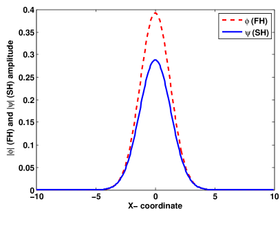
(a)

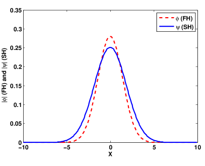
(b)

Figure 1: (Color online) (a) Numerically found profiles of the FH and SH components for a stable 1D soliton, with $Q=-1$, $k=0.32$, $\alpha$ $=0.5$. (b) The same for an unstable 1D soliton, with $Q=-1$, $k=0.28$, $\alpha=0.5$.

In Fig. 2, the family is characterized by the dependence of the total power, $P$, defined as per Eq. (14), on the singular-modulation exponent, $\alpha$, and on the propagation constant, $k$. The results labeled by VA are obtained from the Eqs. (20), (22), and (23), with $\rho$ and $\gamma$ produced by a numerical solution of Eq. (24). Figure 2 demonstrates that the VA provides a reasonable, although imperfect, accuracy, in comparison with the numerical findings.

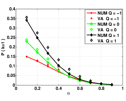
(a)

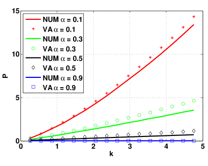
(b)

Figure 2: (Color online) (a) The total power of 1D fundamental solitons, $P$, vs. the singularity exponent, $\alpha$, at a fixed propagation constant, $k=1$, and different values of the mismatch parameter, $Q$. (b) $P(k)$ for $Q=+1$ and several fixed values of $\alpha$. Both numerical results and their counterparts generated by the VA [see Eqs. (19)-(24)] are displayed.

In accordance with what was said above, Fig. 2(a) confirms that solitons indeed vanish at $\alpha=1$ and do not exist at $\alpha>1$. The same figure demonstrates that dependence of the family on mismatch $Q$ [see Eq. (3)] is relatively weak. However, there is an essential difference between $Q=-1$ and $Q=0,+1$, as concerns stability of the solitons, see below. 

An obvious feature observed in Fig. 2(b) (for $Q=+1$) is the positive slope of the curves, i.e., $dP/dk>0$, hence the soliton family satisfies the Vakhitov-Kolokolov (VK) criterion, which is a necessary condition for their stability VK . The same conclusion pertains to the solitons found at $Q=0$, which is actually an exact result, according to Eq. (17). On the other hand, plots $P(k)$ for $Q=-1$, shown in Fig. 3(b), exhibit a region where the VK criterion is not satisfied.

To accurately check the stability of the 1D fundamental solitons, we have computed instability growth rates for eigenmodes of small perturbations added to the stationary solitons (the procedure is described in Appendix A.) This analysis has confirmed that the VK criterion is not only necessary but, as a matter of fact, also sufficient for the stability of the 1D fundamental solitons in the present context. Thus, the solitons are completely stable for $Q=+1$ and $Q=0$, while the boundary between the stable and unstable solitons for $Q=-1$ is shown, in the plane of $\left(k,\alpha\right)$, in Fig. 3(b). In fact, the narrow instability region at $\alpha=0$ is akin to the known narrow instability domain for fundamental 1D solitons in the standard $\chi^{(2)}$ system Quadratic_solitons_Malomed ; Quadratic_solitons .

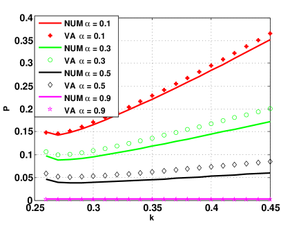
(a)

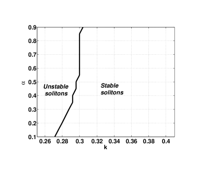
(b)

Figure 3: (a) $P(k)$ for the fundamental 1D solitons with the negative mismatch, $Q=-1$, and several fixed values of the singular-modulation exponent, $\alpha$. This plot demonstrates that there is a region with $dP/dk<0$, where the VK stability criterion does not hold. (b) The stability map for the solitons with $Q=-1$ in the plane of $k$ and $\alpha$ (for $Q=0$ and $Q=+1$, all the fundamental solitons are stable). The instability boundary is produced in the same form by the VK criterion and by the computation of stability eigenvalues for modes of small perturbations.

The predicted stability and instability of the 1D fundamental solitons was also verified by direct simulations. It has been found that, if the integral power (14) of unstable solitons is smaller than the power of their stable counterparts, the unstable solitons suffer complete decay (not shown here in detail). On the other hand, Fig. 4 demonstrates that unstable solitons, whose integral power exceeds that for coexisting stable solitons, do not decay, but rather transform into breathers oscillating around stable solitons.

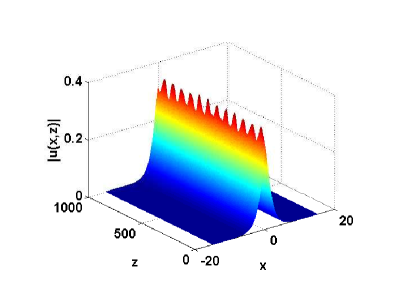
(a)

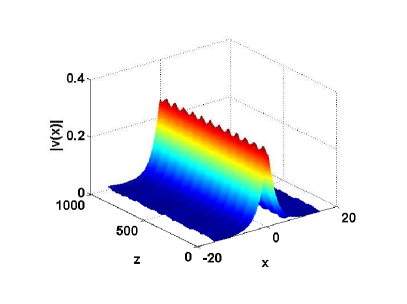
(b)

Figure 4: (Color online) A typical example of the evolution of the FF (a) and SH (b) components of an unstable fundamental soliton, at $k=0.28$, $Q=-1$ and $\alpha=0.5$, whose integral power exceeds that of a co-existing stable soliton $(P>0.04)$. In this case, the evolution leads to the formation of a breather close to the stable soliton.

IV The 1D model with a pair of singular-modulation peaks

To introduce the model with the double-peak spatial modulation, we replace the underlying equations (7), (8) by more general ones,

$$iu_{z}+\frac{1}{2}u_{xx}+g(x)u^{\ast}v=0,$$ (31)

$$2iv_{z}+\frac{1}{2}v_{xx}-Qv+\frac{1}{2}g(x)u^{2}=0,$$ (32)

and select the double-peak modulation function $g(x)$ in the form of

$$g(x)=\left|x-\Delta\right|^{-\alpha}+\left|x+\Delta\right|^{-\alpha},$$ (33)

where the separation between the peaks is $2\Delta$, while the mismatch parameter may be scaled, as above, to one of the three fixed values (3).

Numerical solution of the stationary version of Eqs. (31) and (32) reveals three types of stationary soliton solutions, namely, symmetric ones with maxima separated by distance $2\Delta$, asymmetric solitons, for which the amplitudes are different at $x=+\Delta$ and $-\Delta$, and twisted solitons, in which the FF component is antisymmetric, with opposite amplitudes at $x=\pm\Delta$, while the SH component is symmetric. Typical examples of profiles of all the three types of the solitons are displayed in Fig. 5.

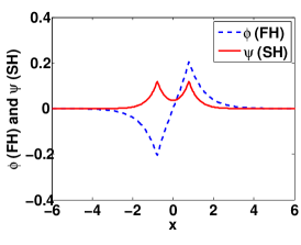
(a)

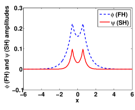
(b)

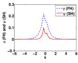
(c)

Figure 5: (Color online) Typical profiles of the FF and SH components of stable 1D solitons supported by the double-peak spatial modulation of the nonlinearity: (a) a twisted soliton ($\Delta=1.17$); (b) a symmetric soliton ($\Delta=0.59$); (c) a strongly asymmetric soliton ($\Delta=0.31$). In all the cases, $Q=+1$, $\alpha=0.5$, and $k=1.2.$ $\Delta$ is the respective value of the half-separation between the peaks.

Similar to other models with two separated symmetric peaks of the local $\chi^{(2)}$ Valery-chi2 and $\chi^{(3)}$ Dong ; Yasha ; Valery nonlinearity strength , the asymmetric solitons are generated from the symmetric ones by the spontaneous-symmetry-breaking bifurcation book , which occurs with the increase of separation $2\Delta$ between the peaks, if other parameters are fixed. The bifurcation is illustrated by Fig. 6, which shows the measure of the asymmetry between the local powers at the two peaks,

$$\Theta\equiv\frac{\left[|u(x=\Delta)|^{2}+4|v(x=\Delta)|^{2}\right]-\left[|u(x=-\Delta)|^{2}+4|v(x=-\Delta)|^{2}\right]}{\left[|u(x=\Delta)|^{2}+4|v(x=\Delta)|^{2}\right]+\left[|u(x=-\Delta)|^{2}+4|v(x=-\Delta)|^{2}\right]},$$ (34)

as a function of the soliton’s wavenumber, for $Q=+1$ (for $Q=0$ and $-1$ the bifurcation diagrams are quite similar). Coordinates of the bifurcation points are summarized in Fig. 7. It is observed that the location of the bifurcation only weakly depends on mismatch $Q$.

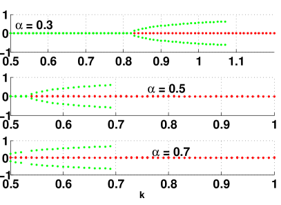
(a)

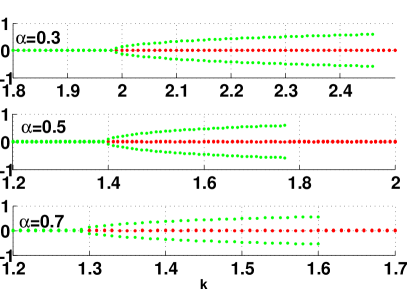
(b)

Figure 6: (Color online) Bifurcation diagrams for the spontaneous symmetry breaking of symmetric solitons supported by the double-peak spatial modulation of the nonlinearity, with separation $2\Delta$ between the peaks and $Q=+1$, at fixed values of the singularity exponent $\alpha$: (a) $\Delta=0.43$; (b) $\Delta=0.27$. Asymmetry parameter (34) is shown vs. wavenumber $k$ of the solitons. Green and red lines depict stable and unstable soliton families, respectively (see the text).

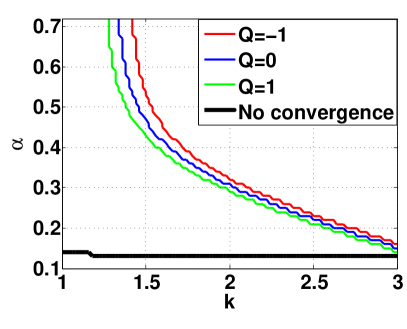
(a)

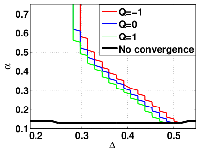
(b)

Figure 7: (Color online) (a) The value of $\alpha$ at the bifurcation point of the spontaneous symmetry breaking of symmetric solitons, vs. their propagation constant $k$, for different values of $Q$ and $\Delta=0.27$, as indicated in the figure. (b) The same for fixed $k=1.2$ and different values of $Q$, $\Delta$ and $\alpha$. The black line bounds the region where the numerical method does not converge to stationary solutions. Here, as well as in Figs. 9(b) and 13 below, red lines are not shown where they overlap with blue ones, and the latter are not shown where they overlap with green lines.

This is a supercritical pitchfork bifurcation Iooss , which destabilizes the symmetric soliton. Accordingly, the accurate analysis of the stability demonstrates that the asymmetric solitons are always stable when they exist, while symmetric ones are stable and unstable when they, respectively, do not or do coexist with the asymmetric solitons. Direct simulations [see Fig. 8] demonstrates that the unstable symmetric solitons spontaneously transform into asymmetric breathers oscillating around coexisting stable asymmetric solitons.

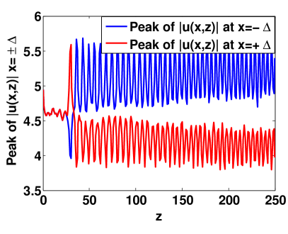
(a)

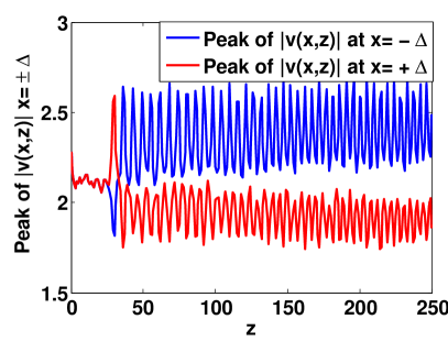
(b)

Figure 8: (Color online) The evolution of peak powers of the two components of an originally unstable symmetric soliton at $\alpha=0.3,\Delta=0.8,Q=1$, and $k=5.5$. The soliton tends to spontaneously rearrange itself into an asymmetric state close to the co-existing asymmetric soliton.

As concerns twisted solitons, they do not undergo breaking of the antisymmetry, and are stable for sufficiently large values of distance $2\Delta$ between the peaks. An example of the stability map for twisted solitons is presented in Fig. (9), which demonstrates that the twisted solitons are stable at $2\Delta\gtrsim 1.5$. In direct simulations, unstable twisted solitons tend to spontaneously transform into stable symmetric or asymmetric ones coexisting with them (not shown here in detail).

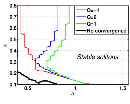
Figure 9: (Color online) The stability map for twisted solitons with different values of $Q$ and fixed wavenumber $k=1$. The solitons are stable at values of $\Delta$ exceeding those corresponding to the displayed boundaries. The region where the numerical method does not converge to a stationary solution is bounded by the black line (the leftmost one).

V Two-dimensional solitons and vortices

V.1 Analytical estimates

In the 2D setting, axially symmetric solutions of stationary equations (5) and (6), with integer vorticity $m$ (fundamental 2D solitons correspond to $m=0$), are looked for, in polar coordinates $\left(r,\theta\right)$, as

$$\varphi(r,\theta)=U(r)e^{im\theta},\psi(r,\theta)=V(r)e^{2im\theta},$$ (35)

with real amplitudes $U(r)$ and $V(r)$ satisfying equations

$$-kU+\frac{1}{2}\left[\frac{1}{r}\frac{dU}{dr}+\frac{d^{2}U}{dr^{2}}-\frac{m^{2}}{r^{2}}U\right]+{r}^{-\alpha}UV=0,$$ (36)

$$-4kV+\frac{1}{2}\left[\frac{1}{r}\frac{dV}{dr}+\frac{d^{2}V}{dr^{2}}-\frac{4m^{2}}{r^{2}}V\right]-QV+\frac{1}{2}{r}^{-\alpha}U^{2}=0,$$ (37)

which can be derived from the Lagrangian [cf. its 1D counterpart (18)]:

$$L=\frac{1}{2}\int_{0}^{\infty}rdr\left\{\frac{1}{2}\left[\left(\frac{dU}{dr}\right)^{2}+\left(\frac{dV}{dr}\right)^{2}\right]+\left[\left(k+\frac{m^{2}}{2r^{2}}\right)U^{2}+\left(4k+\frac{2m^{2}}{r^{2}}+Q\right)V^{2}-r^{-\alpha}U^{2}V\right]\right\}.$$ (38)

The VA for the 2D solitons may be based on the following ansatz (which implies $m\geq 0$),

$$U(r)=Ar^{m}\exp\left(-\rho r^{2}\right),V(r)=Br^{2m}\exp\left(-\gamma r^{2}\right),$$ (39)

cf. the 1D ansatz (19). The substitution of the ansatz into Eq. (38) yields the following effective Lagrangian:

$$\begin{split}L&=\frac{1}{4}\left\{4^{-m}B^{2}m(4k+Q)\gamma^{-1-2m}\Gamma\left(2m\right)+\frac{1}{2}4^{-m}B^{2}\gamma^{-2m}\Gamma\left(2+2m\right)\right\}+\\ &\frac{1}{8}A^{2}\left\{2^{-m}\rho^{-1-m}\left[k\Gamma\left(1+m\right)+\rho\Gamma\left(2+m\right)\right]-2B(\gamma+2\rho)^{-1-2m+\frac{\alpha}{2}}\Gamma\left(1+2m-\frac{\alpha}{2}\right)\right\},\end{split}$$ (40)

where $\Gamma$ is again the Gamma-function, cf. 1D Lagrangian (21). While subsequent analysis can be performed in an explicit form for any integer vorticity $m$, eventually all the vortices with $m\geq 1$ turn out to be unstable, only the fundamental 2D solitons with $m=0$ having a stability area shown below in Fig. 13. Therefore, explicit analytical results  are given here for $m=0$; nevertheless, the VA predictions for vortices have been obtained too, and their comparison with numerical counterparts is presented below in Fig. 12.

The first two variational equations, $\partial L/\partial B=\partial L/\partial\left(A^{2}\right)=0$, if applied to Lagrangian (40), yield expressions for the amplitudes, cf. similar results (22) and (23) for the 1D solitons:

$$A=\frac{\sqrt{(4k+Q+\gamma)(\gamma+2\rho)^{2-\alpha}(k+\rho)}}{\sqrt{2\rho\gamma}\Gamma\left(1-\alpha/2\right)}.$$ (41)

$$B=\frac{(\gamma+2\rho)^{1-\alpha/2}(k+\rho)}{2\rho\Gamma\left(1-\alpha/2\right)},$$ (42)

Taking these results into account, the two remaining variational equations, $\partial L/\partial\rho=\partial L/\partial\gamma=0$, amount, similar to the 1D case [cf. Eq. (24)], to a pair of coupled quadratic equations,

$$\begin{cases}k(\gamma+\alpha\rho)-\left(2-\alpha\right)\rho^{2}=0,\\ \gamma(2-\alpha)\gamma+4k(\gamma-\alpha\gamma-2\rho)+Q(\gamma-\alpha\gamma-2\rho)=0,\end{cases}$$ (43)

which can be solved numerically.

As seen from Eqs. (41) and (42), these results makes sense for $\alpha<2$ (recall in 1D the result was meaningful for $\alpha<1$). Indeed, the average value of the $\chi^{(2)}$ coefficient in a circle of radius $R$ surrounding the singular point is [cf. Eq. (30)]

$$\left\langle\chi^{(2)}\right\rangle_{\mathrm{2D}}\equiv\frac{2}{R^{2}}\int_{0}^{R}r^{1-\alpha}dr=\frac{2}{2-\alpha}R^{-\alpha},$$ (44)

hence the singular nonlinearity-modulation profile may support 2D $\chi^{(2)}$ solitons at $\alpha<2$.

It is possible to analyze the form of the solution at $r\rightarrow 0$, adopting an expansion similar Eq. (25), which was used in the 1D case:

$$\varphi(r)=\varphi_{0}-\varphi_{1}r^{2-\alpha}+...,~{}\psi(x)=\psi_{0}-\psi_{1}r^{2-\alpha}+....$$ (45)

Substituting this into Eqs. (5) and (6), one can easily find

$$\frac{\varphi_{1}}{\varphi_{0}} = \frac{2\psi_{0}}{\left(2-\alpha\right)^{2}},$$ (46)

$$\psi_{1} = \frac{\varphi_{0}^{2}}{\left(2-\alpha\right)^{2}},$$ (47)

cf. the similar 1D relations (27) and (28). Obviously, Eqs. (46) and (47) corroborate that the 2D fundamental solitons exist at $\alpha<2$, as at $\alpha=2$ Eq. (47) dictates $\varphi_{2}=0$, which means that the solution degenerates into a trivial one with a flat SH field and zero FF component.

V.2 Numerical results for 2D solitons and vortices

The Newton’s method, applied to radial equations (36) and (37), with the VA prediction used as the initial guess, readily generates families of axisymmetric fundamental solitons. Solitary vortices can also be found in the numerical form. Typical examples of radial shapes of the fundamental and vortex ($m=1$) solitons are displayed in Fig. 10.

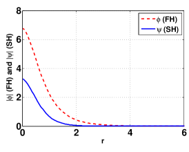
(a)

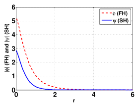
(b)

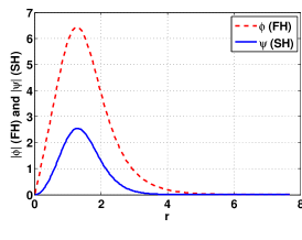
(c)

Figure 10: (Color online) Typical radial profiles of the FF and SH components of 2D solitons. (a) A stable fundamental soliton ($\alpha=0.15,Q=1,k=1$); (b) an unstable fundamental soliton ($\alpha=0.5,Q=1,k=1$); (c) an unstable vortex soliton with $m=1$ ($\alpha=0.15,Q=1,k=1$).

Properties of the 2D soliton families are summarized in Fig. 11.  Note that dependence $P(k)$ for $Q=0$ can be found in the exact form, according to Eq. (17). It is worthy to note that Fig. 11 demonstrates that the accuracy of the VA is actually better for the 2D solitons than for their 1D counterparts, cf. Fig. 2

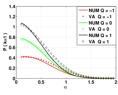
(a)

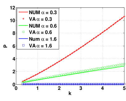
(b)

Figure 11: (Color online) Properties of numerically found fundamental 2D solitons, and their VA-predicted counterparts. (a) The integral power vs. the singular-modulation exponent, $\alpha$, at fixed values of mismatch $Q$, and $k=1$. (b) The integral power vs. $k$ at several fixed values of $\alpha$ and $Q=1$.

For the sake of completeness, we display similar properties of the vortex-soliton family with $m=1$ in Fig. 12, although, as said above, all the vortices are unstable. In this case, the VA still provides a reasonable overall accuracy, although the discrepancy is larger than for the fundamental solitons.

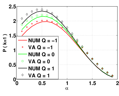
(a)

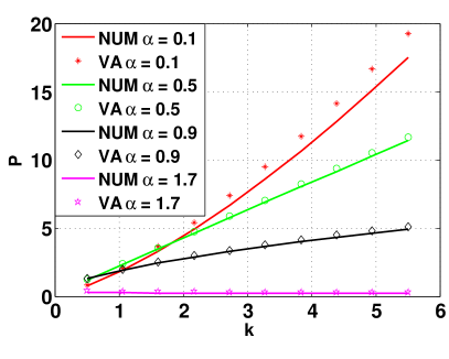
(b)

Figure 12: (Color online) The same as in Fig. 11, but for vortices with $m=1$. The variational results were produced by equations derived from the effective Lagrangian (40).

The stability of the 2D solitons was analyzed by computations of eigenvalues for modes of small perturbations, as described in Appendix B. This analysis yields the following results. First, stability regions for the fundamental 2D solitons are shown in Fig. 13. These solitons are less stable than their 1D counterparts. Indeed, it was demonstrated above that the 1D solitons have an instability region at $Q=-1$ only, see Fig. 3, while the 2D solitons have instability regions for all values of $Q=-1,0,1$. Moreover, it is seen in Fig. 13 that the stability area is slightly larger for $Q=-1$ than for $Q=+1$. Note that, while the 2D fundamental solitons exist up to $\alpha=2$, as shown above, the stability area is limited to $\alpha<0.5$.

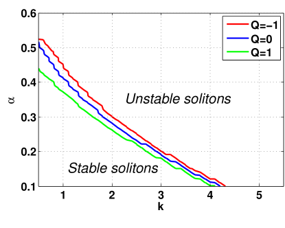
Figure 13: (Color online) The stability map for 2D fundamental solitons.

Direct simulations demonstrate that the instability transforms unstable 2D fundamental solitons into solitary breathers with a small or large amplitude of the intrinsic oscillations, as shown in Figs. 14 and 15, respectively.

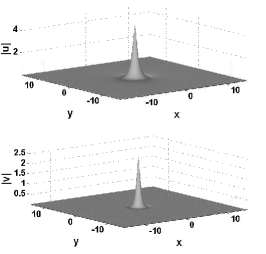
(a)

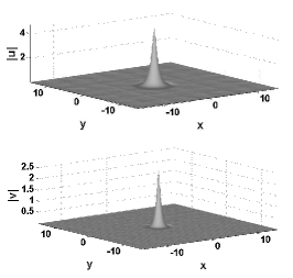
(b)

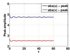
(c)

Figure 14: An example of a breather with a small amplitude of intrinsic oscillations, generated by the instability of a 2D fundamental soliton with $k=1$, $Q=1$ and $\alpha=0.5$. (a,b) Shapes of absolute values of the FF and SH fields at evolution stages corresponding to $z=4$ and $z=40$; (c) peak values of the FH and SH fields as functions of $z$.

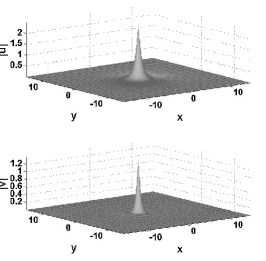
(a)

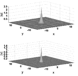
(b)

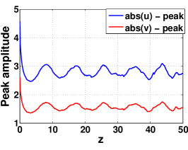
(c)

Figure 15: The same as in Fig. 14, but for a breather with a larger amplitude of intrinsic oscillations, generated by the instability of a fundamental soliton with $k=2$, $Q=1$ and $\alpha=0.8$.

On the other hand, vortex solitons are completely unstable against eigenmodes (60) of azimuthal perturbations, with $J=1$ and $2$ for the vortices with $m=1$, and $J\leq 4$ for $m=2$, similar to the instability of vortex solitons in the uniform $\chi^{(2)}$ medium, which was studied in detail theoretically vort-unstab and demonstrated experimentally experiment . However, direct simulations of Eqs. (1) and (2), which were carried out in the Cartesian coordinates, as shown in Fig. 16, exhibit dynamics very different from that observed in the uniform medium: the instability splits the vortex into three fragments (two large and one smaller), which seem as fundamental solitons. In the course of the subsequent evolution, the fragments do not separate (as they would do in the uniform medium), but feature irregular rotation around the $\chi^{(2)}$ singularity (indeed, the local maximum of the $\chi^{(2)}$ attracts the solitons, as long as they exist). Then, two of them collide and merge into a single soliton. Eventually, the two remaining solitons collide twice: the first time, they bounce from each other, but the second collision leads to their fusion into a single fundamental soliton, which stays pinned to the $\chi^{(2)}$ singularity. The soliton keeps $65\%$ of the total power, being surrounded by a conspicuous field of radiation “debris”, that carries the entire angular momentum (16) (we have checked that the total momentum remains constant in the course of the evolution).

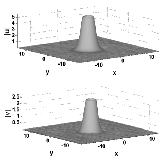
(a)

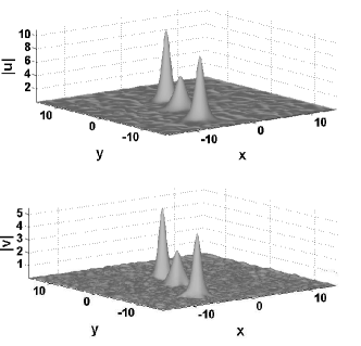
(b)

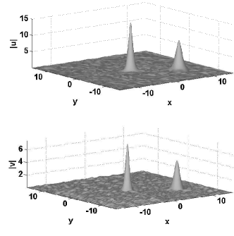
(c)

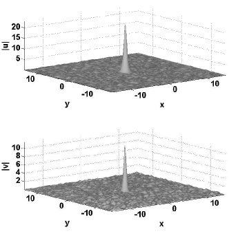
(d)

Figure 16: An example of the instability-induced splitting of the vortex soliton, with $m=1$, $k=1$, $Q=-1$ and $\alpha=0.1$, into a set of three fragments, which is followed by their staged merger into two fundamental solitons, and eventually into a single one, pinned to the $\chi^{(2)}$ singularity. The initial instability of the vortex is dominated by perturbation eigenmode (60) with $J=1$. Panels (a), (b), (c) and (d) display, respectively, shapes of the absolute values of the FF and SH fields at the evolution stages corresponding to $z=20$, $85$, $130$ and $230$ .

VI Conclusion

As a contribution to the currently developing studies of the dynamics of solitons in effective nonlinear potentials, we have introduced a model of second-harmonic-generating media with the local strength of the quadratic nonlinearity featuring the spatial singularity, $\chi^{(2)}\sim|x|^{-\alpha}$ in 1D, and, similarly, $\chi^{(2)}\sim r^{-\alpha}$ in 2D. The spatial modulation of the nonlinearity can be implemented experimentally with the help of the poling technique. We have found, using analytical and numerical methods, that the robust fundamental solitons, pinned to the singularity points, exist at $\alpha<1$ and $\alpha<2$, respectively, in the 1D and 2D cases (the $\chi^{(3)}$ counterpart of the 1D system, related to it by the cascading limit, supports solitons in a narrower region, $\alpha<1/2$). The 1D solitons are stable, except for a narrow domain in the parameter space, while the 2D fundamental solitons are stable at $\alpha<1/2$. A noteworthy fact is that the variational approximation provides more accurate results for the 2D fundamental solitons than for their 1D counterparts. In the 2D setting, vortex solitons have been constructed too. They are unstable against splitting, but in a way different from the known instability scenario in the uniform $\chi^{(2)}$ medium: typically, the unstable vortex splits into three fragments, which eventually merge into a single soliton pinned to the central singularity. In the 1D system, we have also studied the spontaneous symmetry breaking of solitons pinned to a pair of singular-modulation peaks, which gives rise to nontrivial asymmetric pinned modes via the supercritical bifurcation.

As a development of the present work, it may be interesting to study the symmetry breaking in the 2D system with two or three symmetrically placed singular peaks, the latter configuration being an especially interesting one Pfau .

Appendix A Eigenmodes stability analysis of 1D model

The stability of perturbed stationary solutions can be evaluated by calculation of eigenvalues for modes of small perturbations. The perturbed solutions of Eqs. (7), (8) are introduced as

$$u_{p} = \left[\varphi(x)+(\epsilon_{\varphi R}+i\epsilon_{\varphi I})\right]e^{ikz},$$ (48)

$$v_{p} = \left[\psi(x)+(\epsilon_{\psi R}+i\epsilon_{\psi I})\right]e^{2ikz},$$ (49)

where $\epsilon_{\varphi R}$, $\epsilon_{\psi R}$ and $\epsilon_{\varphi I}$, $\epsilon_{\psi I}$ are real and imaginary parts of the perturbations. Substituting $u_{p}$ and $v_{p}$ into Eqs. (7), (8), we arrive at the system of linearized equations

$$i\epsilon_{\varphi_{z}}-k(\varphi_{0}+\epsilon_{\varphi})+\frac{1}{2}(\varphi_{0_{xx}}+\epsilon_{\varphi_{xx}})+{\left|x\right|}^{-\alpha}(\varphi_{0}+\epsilon_{\varphi})^{\ast}(\psi_{0}+\epsilon_{\psi}) = 0,$$ (50)

$$2i\epsilon_{\psi_{z}}-4k(\psi_{0}+\epsilon_{\psi})+\frac{1}{2}(\psi_{0_{xx}}+\epsilon_{\psi_{xx}})-Q(\psi_{0}+\epsilon_{\psi})+\frac{1}{2}{\left|x\right|}^{-\alpha}(\varphi_{0}+\epsilon_{\varphi})^{2} = 0,$$ (51)

where $\varphi_{0}$ and $\psi_{0}$ are stationary solutions found by means of the Newton’s method, $\varphi_{0}=u(x,z)_{z=0}$ and $\psi_{0}=v(x,z)_{z=0}$, while $\epsilon_{\varphi}$ , $\epsilon_{\psi}$ are complex perturbations. Further, the two complex coupled linearized equation can be rewritten, in the matrix form, as a system of four real equations:

$$\left[\begin{array}[]{c}\epsilon_{\varphi R}\\ \epsilon_{\varphi I}\\ \epsilon_{\psi R}\\ \epsilon_{\psi I}\end{array}\right]_{z}=\begin{bmatrix}0&A&0&-B\\ C&0&B&0\\ 0&-D&0&E\\ D&0&-E&0\end{bmatrix}\times\left[\begin{array}[]{c}\epsilon_{\varphi R}\\ \epsilon_{\varphi I}\\ \epsilon_{\psi R}\\ \epsilon_{\psi I}\end{array}\right],$$ (52)

with definitions

$$A \equiv k-\frac{1}{2}D^{(2)}+\mathrm{diag}({\left|x_{i}\right|}^{-\alpha}(\psi_{0_{i}})),$$ (53)

$$B \equiv \mathrm{diag}({\left|x_{i}\right|}^{-\alpha}(\varphi_{0_{i}})),$$ (54)

$$C = -k+\frac{1}{2}D^{(2)}+\mathrm{diag}({\left|x_{i}\right|}^{-\alpha}(\psi_{0_{i}})),$$ (55)

$$D \equiv \mathrm{diag}(\frac{1}{2}{\left|x_{i}\right|}^{-\alpha}(\varphi_{0_{i}})),$$ (56)

$$E \equiv 2k-\frac{1}{4}D^{(2)}+\frac{1}{2}Q.$$ (57)

Replacing $D^{(2)}$ by the differentiation matrix and calculating eigenvalues of resulting matrix (52), the stability can be examined.

Appendix B Eigenmodes stability analysis of 2D model

The stability analysis for the 2D model was performed by taking perturbed solutions as

$$u = \left[U(r)+\epsilon_{u}(z,r,\theta)\right]e^{i\left(m\theta+kz\right)}$$ (58)

$$v = \left[V(r)+\epsilon_{v}(z,r,\theta)\right]e^{2i\left(m\theta+kz\right)}$$ (59)

and looking for perturbation eigenmodes with their own integer vorticity, $J$, which is independent of $m$:

$$\begin{cases}\epsilon_{u}=\xi_{J}^{+}(r)e^{i(\lambda z+J\theta)}+\xi_{J}^{-}(r)e^{-i(\lambda^{\ast}z+J\theta)},\\ \epsilon_{v}=\xi_{J}^{+}(r)e^{i(\lambda z+J\theta)}+\xi_{J}^{-}(r)e^{-i(\lambda^{\ast}z+J\theta)},\end{cases}$$ (60)

where $\lambda$ is the respective eigenvalue (that may be complex), instability corresponding to $\mathrm{Im}(\lambda)\neq 0$. Numerical solution of the eigenvalue problem, generated by the linearization of Eqs. (1), (2) with respect to the small perturbations, produces the following characteristic matrix:

$$G=\begin{bmatrix}J_{+}&A&B&0\\ -A&J_{-}&0&-B\\ \frac{B}{2}&0&E_{+}&0\\ 0&-\frac{B}{2}&0&E_{-}\end{bmatrix},$$ (61)

where we define

$$J_{+} \equiv -k+\frac{1}{2}\left[{\rm diag}(\frac{1}{r_{i}})D^{(1)}+D^{(2)}-{\rm diag}(\frac{1}{r_{i}^{2}})(J+m)^{2}\right],$$

$$J_{-} \equiv k-\frac{1}{2}\left[{\rm diag}(\frac{1}{r_{i}})D^{(1)}+D^{(2)}-{\rm diag}(\frac{1}{r_{i}^{2}})(J-m)^{2}\right],$$

$$E_{+} \equiv -2k+\frac{1}{4}\left[{\rm diag}(\frac{1}{r_{i}})D^{(1)}+D^{(2)}-{\rm diag}(\frac{1}{r_{i}^{2}})(J+2m)^{2}\right]-\frac{1}{2}Q,$$

$$E_{-} \equiv 2k-\frac{1}{4}\left[{\rm diag}(\frac{1}{r_{i}})D^{(1)}+D^{(2)}-{\rm diag}(\frac{1}{r_{i}^{2}})(J-2m)^{2}\right]+\frac{1}{2}Q,$$

$$A \equiv {\rm diag}(r_{i}^{-\alpha}V_{0_{i}}),$$

$$B \equiv {\rm diag}(r_{i}^{-\alpha}U_{0_{i}})$$ (62)

Here $D^{(1)}$ and $D^{(2)}$ are the first- and second-order differentiation matrices. In this case the solution is unstable if there is eigenvalue of $G$ with $\mathrm{Im}(\lambda)\neq 0$.

References

- (1) J. Yang, Nonlinear Waves in Integrable and Nonintegrable Systems (SIAM: Philadelphia, 2010); D. E. Pelinovsky, Localization in Periodic potentials (Cambridge University Press, Cambridge, 2011).
- (2) W. A. Harrison, Pseudopotentials in the Theory of Metals (Benjamin: New York, 1966).
- (3) Y. V. Kartashov, B. A. Malomed, and L. Torner, Rev. Mod. Phys. 83, 247 (2011).
- (4) J. Hukriede, J., D. Runde, and D. Kip, J. Phys. D 36, R1 (2003).
- (5) Y. Kominis, Phys. Rev. E 73, 066619 (2006); Y. Kominis, and K. Hizanidis, Opt. Lett. 31, 2888 (2006); Opt. Exp. 16, 12124 (2008).
- (6) P. O. Fedichev, Y. Kagan, G. V. Shlyapnikov, and J. T. M. Walraven, Phys. Rev. Lett. 77, 2913 (1996); M. Theis, G. Thalhammer, K. Winkler, M. Hellwig, G. Ruff, R. Grimm, and J. H. Denschlag, ibid. 93, 123001 (2004); M. Yan, B. J. DeSalvo, B. Ramachandhran, H. Pu, and T. C. Killian, ibid. 110, 123201 (2013).
- (7) K. Henderson, C. Ryu, C. MacCormick, and M. G. I. Boshier, New J. Phys. 11, 043030 (2009); C. Ryu, P. W. Blackburn, A. A. Blinova, and M. G. Boshier, Phys. Rev. Lett. 111, 205301 (2013).
- (8) H. S. Ghanbari, T. D. Kieu, A. Sidorov, and P. Hannaford, J. Phys. B: At. Mol. Opt. Phys. 39, 847 (2006); O. Romero-Isart, C. Navau, A. Sanchez, P. Zoller, and J. I. Cirac, Phys. Rev. Lett. 111, 145304 (2013); S. Ghanbari, A. Abdalrahman, A. Sidorov, and P. Hannaford, J. Phys. B: At. Mol. Opt. Phys. 47, 115301 (2014); S. Jose, P. Surendran, Y. Wang, I. Herrera, L. Krzemien, S. Whitlock, R. McLean, A. Sidorov, and P. Hannaford, Phys. Rev. A 89, 051602 (2014).
- (9) B. A. Malomed and M. Y. Azbel, Phys. Rev. B 47, 10402 (1993).
- (10) M. I. Molina and G. P. Tsironis, Phys. Rev. B 47, 15330 (1993); B.C. Gupta, and K. Kundu, ibid. 55, 894 (1997).
- (11) V. A. Brazhnyi and B. A. Malomed, Phys. Rev. A 83, 053844 (2011); Opt. Commun. 324, 277 (2014).
- (12) B. Maes, M. Soljačić, J. D. Joannopoulos, P. Bienstman, R. Baets, S.-P. Gorza, and M. Haelterman, Opt. Express14, 10678 (2006); E. N. Bulgakov and A. F. Sadreev, Phys. Rev. B 81, 115128 (2010); E. Bulgakov, A. Sadreev, and K. N. Pichugin, ibid. 83, 045109 (2011).
- (13) O. V. Borovkova, V. E. Lobanov, and B. A. Malomed, Phys. Rev. A 85, 023845 (2012).
- (14) L. Bergé, Phys. Rep. 303, 259 (1998); C. Sulem and P.-L. Sulem, The Nonlinear Schrödinger Equation (Springer: Berlin, 1999); G. Fibich and G. Papanicolaou, SIAM J. Appl. Math. 60, 183 (1999); E. A. Kuznetsov and F. Dias, Phys. Rep. 507, 43 (2011).
- (15) R. A. Myers, N. Mukherjee, and S. R. J. Brueck, Opt. Lett. 16, 1732 (1991); S. Brasselet and J. Zyss, J. Opt. Soc. Am. B 15, 257 (1998).
- (16) C. Etrich, F. Lederer, B. A. Malomed, T. Peschel, and U. Peschel, Progr. Optics 41, 483 (2000).
- (17) A. V. Buryak, P. Di Trapani, D. V. Skryabin, and S. Trillo, Phys. Rep. 370, 63 (2002).
- (18) M. M. Fejer, G. A. Magel, D. H. Jundt, and R. L. Byer, IEEE J. Quant. Electr. 28, 2631 (1992); M. Yamada, N. Nada, M. Saitoh, and K. Watanabe, Appl. Phys. Lett. 62, 435; V. Berger, Phys. Rev. Lett. 81, 4136(1998).
- (19) R. Lifshitz, A. Arie, and A. Bahabad, Phys. Rev. Lett. 95, 133901 (2005); A. Arie, N. Habshoosh, and A. Bahabad, Opt. Quant. Electr. 39, 361 (2007); A. Arie and N. Voloch, Laser Phot. Rev. 4, 355 (2010).
- (20) A. A. Sukhorukov and Y. S. Kivshar, Phys. Rev. E 65, 036609 (2002).
- (21) A. Shapira, N. Voloch-Bloch, B. A. Malomed, and A. Arie, J. Opt. Soc. Am. B 28, 1481 (2011).
- (22) V. A. Brazhnyi and B. A. Malomed, Phys. Rev. A 86, 013829 (2012).
- (23) Y. V. Kartashov, V. V. Konotop, V. A. Vysloukh, and D. A. Zezyulin, in: Spontaneous Symmetry Breaking, Self-Trapping, and Josephson Oscillations, ed. by B. A. Malomed (Springer: Heidelberg, 2013); B. A. Malomed, J. Opt. Soc. Am. B 31, 2460 (2014).
- (24) V. E. Lobanov, O. V. Borovkova, and B. A. Malomed, Phys. Rev. A 90, 053820 (2014).
- (25) Y. V. Kartashov, V. V. Konotop, V. A. Vysloukh, and D. A. Zezyulin, in: Spontaneous Symmetry Breaking, Self-Trapping, and Josephson Oscillations, ed. by B. A. Malomed (Springer 2013).
- (26) B. A. Malomed, J. Opt. Soc. Am. B 31, 2460 (2014).
- (27) Spontaneous Symmetry Breaking, Self-Trapping, and Josephson Oscillations, Editor: B. A. Malomed (Springer-Verlag: Berlin and Heidelberg, 2013).
- (28) J. Yang, B. A. Malomed, and D. J. Kaup,Phys. Rev. Lett. 83, 1958 (1999); A. R. Champneys, B. A. Malomed, J. Yang, and D. J. Kaup, Physica D 152-153, 340 (2001).
- (29) V. Steblina, Yu. S. Kivshar, M. Lisak, and B. A. Malomed, Opt. Commun. 118, 345 (1995).
- (30) G. Iooss and D. D. Joseph, Elementary Stability and Bifurcation Theory (Springer: New York, 1980).
- (31) W. J. Firth and D. V. Skryabin, Phys. Rev. Lett. 79, 2450 (1997); L. Torner and D. V. Petrov, Electron. Lett. 33, 608- (1997); D. V. Skryabin and W. J. Firth, Phys. Rev. E 58, R1252 (1998); J. P. Torres, J. M. Soto-Crespo, L. Torner, and D. V. Petrov, J. Opt. Soc. Am. B 15, 625 (1998); ; J. P. Torres, J. M. Soto-Crespo, L. Torner, and D. V. Petrov, Opt. Commun. 149, 77 (1998).
- (32) D. V. Petrov, L. Torner, J. Martorell, R. Vilaseca, J. P. Torres, and C. Cojocaru, Opt. Lett. 23, 1444 (1998).
- (33) T. Mayteevarunyoo, B. A. Malomed, and G. Dong, Phys. Rev. A 78, 053601 (2008).
- (34) A. Acus, B. A. Malomed, and Y. Shnir, Physica D 241, 987 (2012).
- (35) N. Dror and B. A. Malomed, Phys. Rev. A 83, 033828 (2011).
- (36) T. Lahaye, T. Pfau, and L. Santos, Phys. Rev. Lett. 104, 170404 (2010).