Free energies of molecular clusters determined by guided mechanical disassembly

Abstract

The excess free energy of a molecular cluster is a key quantity in models of the nucleation of droplets from a metastable vapour phase; it is often viewed as the free energy arising from the presence of an interface between the two phases. We show how this quantity can be extracted from simulations of the mechanical disassembly of a cluster using guide particles in molecular dynamics. We disassemble clusters ranging in size from 5 to 27 argon-like Lennard-Jones atoms, thermalised at 60 K, and obtain excess free energies, by means of the Jarzynski equality, that are consistent with previous studies. We only simulate the cluster of interest, in contrast to approaches that require a series of comparisons to be made between clusters differing in size by one molecule. We discuss the advantages and disadvantages of the scheme and how it might be applied to more complex systems.

I Introduction

The formation of droplets from a metastable vapour phase is a commonplace event in nature, but so far it has resisted quantitative analysis, despite repeated attention Kashchiev (2000); Ford (2004); Vehkamäki (2006); Kalikmanov (2013). The phenomenon plays a role in atmospheric aerosol and cloud formation Zhang et al. (2011); Kulmala et al. (2014), as well as in industrial processes Agranovski (2010); Bakhtar et al. (1995). Theoretical analysis often begins with the Becker-Döring equations Becker and Döring (1935) that describe changes in the populations $n_{i}$ of clusters of $i$ molecules brought about by the processes of gain and loss of single molecules, or monomers. They take the form

$$dn_{i}/dt=\beta_{i-1}n_{i-1}+\alpha{}_{i+1}n_{i+1}-\left(\beta_{i}+\alpha_{i}\right)n_{i},$$ (1)

where $\beta_{i}$ and $\alpha_{i}$ are growth and evaporation rates, respectively. The rate of nucleation $J$ of droplets from a metastable vapour phase may then be expressed as Ford (1997)

$$J=n_{1}\beta_{i^{*}}Z\exp\left[-\left(\phi(i^{*})-\phi(1)\right)/kT\right],$$ (2)

where $k$ is the Boltzmann constant, $T$ is the temperature, $i^{*}$ is the size of the critical cluster, defined to have equal probabilities, per unit time, of molecular gain or loss, and $Z$ is the Zeldovich factor that accounts for the nonequilibrium nature of the kinetics Zeldovich (1942). We shall refer to $\phi(i)$ as the thermodynamic work of formation of a cluster of $i$ particles (or $i$-cluster) starting from the metastable vapour phase. A range of nomenclature is used for this quantity in the nucleation theory literature: the work of formation was denoted by $\epsilon(i)$ in Ford (1997), and elsewhere the same, or a very similar quantity has been labelled as $\Delta F$, $\Delta G$ or $\Delta W$, for example.

We note that $\phi$ in the nucleation rate expression has both a kinetic and a thermodynamic interpretation Ford and Harris (2004). The quantity $\phi(i)-\phi(1)$ can be expressed in terms of ratios of cluster growth and evaporation rates:

$$\phi(i)-\phi(1)=-kT\sum\limits_{j=2}^{i}\ln\frac{\beta_{j-1}}{\alpha_{j}},$$ (3)

but $\phi$ is also related to the grand potential $\Omega_{s}(i)=F(i)-i\mu_{s}$ of an $i$-cluster at the chemical potential $\mu_{s}$ of the saturated vapour Ford (1997):

$$\phi(i)=\Omega_{s}(i)-ikT\ln S,$$ (4)

where $F(i)$ is the Helmholtz free energy of the cluster, $S=p_{v}/p_{vs}$ is the vapour supersaturation, and $p_{v}$ and $p_{vs}$ are the vapour pressure and saturated vapour pressure, respectively. The role of the grand potential in this context is to specify the equilibrium population of clusters of size $i$ in a saturated vapour, namely $n_{i}^{s}=\exp(-\Omega_{s}(i)/kT)$. The nucleation model is completed by representing the population of monomers as $n_{1}=Sp_{vs}V/kT$, where $V$ is the system volume, by assuming that the vapour pressure is dominated by the ideal partial pressure of single molecules.

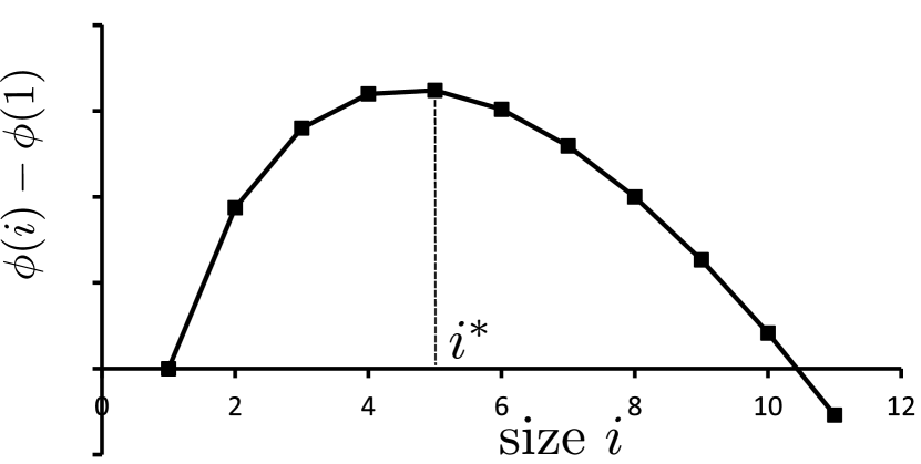
Figure 1: Typical work of formation of a cluster of $i$ particles with a maximum at the critical cluster size $i^{*}$.

In classical nucleation theory (CNT), clusters are viewed as scaled down versions of macroscopic droplets. According to this approach, the difference $\phi(i)-\phi(1)$ is replaced by $\phi(i)$ alone with

$$\phi(i)\approx\phi_{{\rm cl}}(i)=\gamma A(i)-ikT\ln S,$$ (5)

where $\gamma$ is the surface tension of a planar interface between vapour and condensate, and $A(i)$ is the surface area of a cluster represented as a sphere with a density equal to that of the bulk condensed phase. The work of formation is a combination of a free energy cost of forming the interface, and a free energy return proportional to the number of molecules in the cluster (or proportional to its volume since the condensed phase density is taken to be a constant). The neglected $\phi(1)$ term might be represented by $\gamma A(1)-kT\ln S$, which leads to the internally consistent classical theory Girshick and Chiu (1990).

The cluster size dependence of the CNT work of formation is illustrated in Figure 1. It represents a thermodynamic barrier, with a maximum at the critical size, that limits the natural tendency for small molecular clusters to grow into large droplets when exposed to a supersaturated vapour. CNT has been modified in several ways, for example by introducing a size-dependent surface tension Tolman (1949) or by introducing compatibility with nonideal vapour properties Laaksonen et al. (1994); Kalikmanov and van Dongen (1995).

More fundamentally, the ratio of kinetic coefficients $\beta_{j-1}/\alpha_{j}$ might be evaluated using an underlying microscopic model for all clusters up to the critical size and beyond Ford and Harris (2004), and the work of formation determined through Eq. (3). It may be shown that

$$\beta_{j-1}/\alpha_{j}=S\exp\left[-[\Omega_{s}(j)-\Omega_{s}(j-1)]/kT\right],$$ (6)

which shifts attention to the free energy difference $F(j)-F(j-1)$ associated with the addition of a molecule to a $(j-1)$-cluster. Computing these differences is the basis of an approach has been used extensively in calculations of cluster free energies Lee et al. (1973); Hale and Ward (1982); ten Wolde and Frenkel (1998); Oh and Zeng (1999); Kusaka and Oxtoby (2000); Chen et al. (2001); Merikanto et al. (2004). But nucleation is actually controlled by the properties of clusters near the critical size, and one drawback of computing the differences $F(j)-F(j-1)$ is that the predicted nucleation rate could be susceptible to the accumulation of errors in evaluating such a sequence.

In this paper, we describe a computational method for directly obtaining the cluster free energy without the need to perform calculations for a sequence of smaller clusters. We consider the following representation of the work of formation of a cluster minus that of a monomer:

$$\phi(i)-\phi(1)=F_{s}(i)-(i-1)kT\ln S.$$ (7)

We shall refer to $F_{s}(i)$ as the cluster excess free energy, though more accurately it is a difference between the excess free energies of an $i$-cluster and a monomer Ford (1997). It is ‘excess’ in that it represents the free energy required to carve a cluster out of a bulk condensed phase, or equivalently to assemble it out of saturated vapour. It may be associated with the thermodynamic cost of creating an interface, which is why in CNT it is modelled by a surface term, and why we have given it a suffix $s$.

Our approach centres on disassembling a cluster into its component molecules using guided molecular dynamics in order to calculate the cluster excess free energy directly. The method employs the Jarzynski equality Jarzynski (1997a, b); Spinney and Ford (2012) and we provide details in Section II, including a comparison with the related method of thermodynamic integration. Tests of the method where we separate a dimer according to a variety of protocols are described in Appendix A. The disassembly of argon-like Lennard-Jones clusters is presented in Section III and we compare our results with those obtained from Monte Carlo studies by Barrett and Knight Barrett and Knight (2008) and Merikanto $et\,al.$ Merikanto et al. (2006, 2007). These studies gave consistent excess free energies, though they were not in agreement with experiments by Iland $et\,al.$ Iland et al. (2007). We conclude with a discussion of the advantages and disadvantages of the approach compared with other treatments in Section IV.

II Guided molecular dynamics simulations

II.1 Fundamentals of the method

We study the dynamical evolution of a cluster against a background of external manipulation. The cluster particles are harmonically tethered to a set of artificial ‘guide particles’, which lie initially at the origin but after a period of system equilibration are programmed to move apart, driving cluster disassembly. The strength of the tether forces is initially quite weak, in order to disturb the properties of the cluster as little as possible. Later, the tethers can be strengthened in order to guide the separation process more firmly, and to prevent the atoms from interacting with each other once the final guide particle positions have been reached. The mechanical work of the disassembly can then be related to the change in Helmholtz free energy.

The masses of the guide particles are taken to be very much greater than those of the cluster particles. This essentially fixes the trajectories of the guide particles in the molecular dynamics, in accordance with the velocities assigned to each at the beginning of the disassembly process. By choosing guide particle velocities, simulation times and a time-dependent tethering force, a range of cluster disassembly protocols can be explored. A simple illustration of the process is shown in Figure 2.

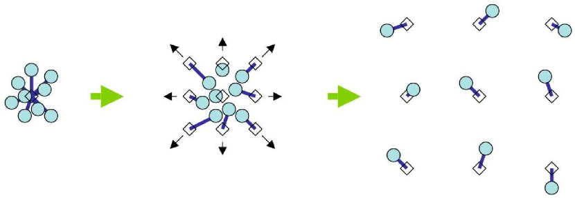
Figure 2: Guided disassembly process for an $i$-cluster. The real particles (circles) are initially weakly tethered to the guide particles (diamonds). The latter drift apart and the tethers gradually tighten leading to $i$ independent, tethered particles upon completion of the process.

We shall consider clusters of argon-like atoms interacting through Lennard-Jones potentials, and so we shall refer to the cluster particles as atoms. We equilibrate this system under the influence of the tethers for a suitable period, the duration of which will depend upon the cluster size and the desired temperature. A further molecular dynamics simulation is performed and from this trajectory we select initial configurations for cluster disassembly. In order that the configurations should represent a bound structure, we employ a Stillinger cluster condition Stillinger (1963) in the selection, allowing a separation of no more than $1.5\,\sigma_{{\rm ArAr}}$ between an atom and its nearest neighbour, where $\sigma_{{\rm ArAr}}$ is the usual Lennard-Jones range parameter. Such a Stillinger condition has been used in previous Monte Carlo approaches. The cluster definition is an important ingredient of a modelling strategy Ford (2004), and deserves careful consideration, but here we shall use this simple criterion for convenience.

The simulations were performed using the DL_POLY Smith et al. (1996) molecular dynamics package, with modifications to the source code to implement the time-dependent harmonic tether potentials. We include a physical heat bath of helium-like Lennard-Jones atoms thermalised using a Nosé-Hoover thermostat Tang and Ford (2006). We could instead have implemented a thermostat that acts on the cluster itself, but chose not to in order to achieve as natural a thermalisation as possible during the nonequilibrium processing.

II.2 Work performed on a system

Given an external control parameter $\lambda$ in a Hamiltonian $H(\lambda)$, the work $W$ done on a system due to the evolution of $\lambda$ over a finite time period may be written

$$W=\int\frac{d\lambda}{dt}\frac{\partial H(\lambda)}{\partial\lambda}dt.$$ (8)

For example, consider the Hamiltonian $H_{1}$ of a single guided atom of mass $m$:

$$H_{1}=\frac{\boldsymbol{p}^{2}}{2m}+\frac{1}{2}\kappa(t)\left[\boldsymbol{x}(t)-\mathbf{X}(t)\right]^{2},$$ (9)

where $\boldsymbol{p}$ is the momentum, $\kappa(t)$ is the time-dependent tethering force or spring constant, $\boldsymbol{x}(t)$ is the atomic position and $\mathbf{X}(t)$ is the guide position. For a set of guided atoms, each controlled by a Hamiltonian $H$ containing terms of the form given in Eq. (9) supplemented by interparticle interactions, $\kappa(t)$ and $\mathbf{X}(t)$ play the role of $\lambda$ and the work $W$ performed on the set is

$$\int\limits_{0}^{\tau}\frac{d\kappa(t)}{dt}\frac{\partial H(\kappa,\{\mathbf{X}_{k}\})}{\partial\kappa}dt+\sum_{j}\int\limits_{0}^{\tau}\frac{d\mathbf{X}_{j}(t)}{dt}\frac{\partial H(\kappa,\{\mathbf{X}_{k}\})}{\partial\mathbf{X}_{j}}dt$$ (10)

$$=\frac{1}{2}\int\limits_{0}^{\tau}\frac{d\kappa(t)}{dt}\sum_{j=1}^{i}\left[\boldsymbol{x}_{j}(t)-\mathbf{X}_{j}(t)\right]^{2}dt$$

$$-\int\limits_{0}^{\tau}\kappa(t)\sum_{j=1}^{i}\left[\boldsymbol{x}_{j}(t)-\mathbf{X}_{j}(t)\right]\cdot\mathbf{V}_{j}(t)dt,$$

where $\tau$ is the length of the molecular dynamics simulation, and $\mathbf{V}_{j}(t)$ is the velocity of the guide particle associated with the $j^{{\rm th}}$ atom, defined as $\mathbf{V}_{j}(t)=d\mathbf{X}_{j}(t)/dt$. The first term in Eq. (10) arises from the time dependence of the spring constant, and the second term is simply the conventional force times distance expression. It should be noted that all tethers within the system are characterised by the same spring constant, although more elaborate protocols could be imagined.

II.3 The Jarzynski equality

If we were able to perform an extremely slow, quasistatic process, then the mechanical work done would be equal to the difference in Helmholtz free energy between the initial and final equilibrium states. However, quasistatic processes are unfeasible in finite time molecular dynamics simulations and according to the second law Ford (2013), the average of the work done (as a result of a time-dependent change in the Hamiltonian of the system), performed over many realisations of a nonquasistatic process (indicated by angled brackets), will always be an overestimate of the free energy change, $\left\langle W\right\rangle>\Delta F$, allowing us only to infer an upper limit to $\Delta F$.

However, the Jarzynski equality Jarzynski (1997a, b)

$$\left<\exp\left(-W/kT\right)\right>=\exp\left(-\Delta F/kT\right)$$ (11)

allows us to do better. For this identity to hold, the system must begin in thermal equilibrium, but need not remain so as the Hamiltonian changes during the simulation. Exploiting the work done in a nonequilibrium process is a powerful strategy for calculating cluster surface free energies and numerous computational studies Hendrix and Jarzynski (2001); Hummer (2002); Hu et al. (2002); Rodriguez-Gomez et al. (2004); Lua and Grosberg (2005); Dhar (2005); Palmieri and Ronis (2007) as well as experiments Hummer (2001); Ritort et al. (2002); Liphardt et al. (2002); Collin et al. (2005); Douarche et al. (2005); Joubaud et al. (2007) have achieved this with the help of the Jarzynski equality. Systems studied include argon-like Lennard-Jones fluids, ion-charging in water, ideal gases confined to a piston, and one-dimensional polymer chains. Nevertheless, there are distinct aspects of this strategy for analysing the controlled disassembly of a cluster that need to be explored.

The Jarzynski equality ought to recover the free energy difference regardless of the nature of the evolution between initial and final Hamiltonians, but computed results might still depend upon the rate of the process as a consequence of a limited sampling of system trajectories in finite simulations Hummer (2001). We might expect ‘slow’ processes that gently pull a cluster apart to generate a narrower distribution of work compared with ‘fast’ processes that are violent and highly dissipative. A balance must therefore be struck between the poorer convergence of fast simulations and the demand for computational resources required for slow simulations.

Furthermore, a consequence of the exponential averaging in the Jarzynski equality is that occasional values of work that are well below the average, arising from unusual trajectories, can sometimes distort the extracted free energy change. This is a consequence of insufficient sampling of the system trajectories and so we need to give careful attention to the statistical errors.

We have explored the outcomes of various guiding protocols, and the robustness of the Jarzynski equality in the face of limited statistics, in a test case of the separation of a dimer, for which the free energy change is easily calculable. These studies are described in Appendix A. We have used similar protocols to study the disassembly of larger clusters, which is described in Section III.

II.4 Comparison with thermodynamic integration

The method bears some similarity to thermodynamic integration, where the strength of the interparticle interactions is evolved over a sequence of equilibrium calculations in order to compare the system in question with another that has a known free energy Kirkwood (1935); Straatsma et al. (1986); Miller and Reinhardt (2000); Schilling and Schmid (2009). The basic relationship $\Delta F=\int\langle\partial H(\lambda)/\partial\lambda\rangle d\lambda$ is analogous to Eq. (8). The reference system for clusters might, for example, be a set of noninteracting particles held together through the retention of the constraining cluster definition. Or indeed the cluster definition could be changed progressively along with the interactions in order to reach a more convenient final state, perhaps noninteracting particles inside a sphere.

However, there are some important differences. In our approach it is the tether potentials that change with time, not the interparticle interactions, and our reference system is a set of independent harmonic oscillators, not an ideal gas. Furthermore, we conduct the evolution by nonequilibrium molecular dynamics rather than by moving through a sequence of equilibrium ensembles, and we only need to impose a cluster definition when selecting the initial configurations, not throughout the evolution. An abrupt removal of the cluster definition constraint is acceptable in a nonequilibrium evolution, when the results are processed using the Jarzynski equation, but it would not be appropriate during a sequence of equilibrium calculations.

III Argon cluster disassembly

III.1 Preliminaries

We have investigated the disassembly of clusters consisting of 5, 10, 15, 20 and 27 argon-like atoms in order to obtain their excess free energies. Scaling up the guided molecular dynamics simulations from the test case of dimer separation is fairly straightforward. We perform simulations in a cubic cell with edge lengths of 100 Å, so that the initial clusters and the final disassembled configurations may be easily accommodated. We employ Lennard-Jones interaction potentials for each species (see Table 3) and the helium temperature is set at 60 K in order to facilitate a comparison with the Monte Carlo studies by Barrett and Knight Barrett and Knight (2008) and Merikanto $et\,al.$ Merikanto et al. (2006, 2007), as well as the experimental studies of Iland $et\,al.$ Iland et al. (2007).

However, converting the free energy change associated with disassembly into an excess free energy requires some careful consideration of the statistical mechanics of tethered and free molecular clusters. We require the excess free energy of a cluster that is free to move anywhere inside a system volume, but our initial state is a cluster tethered to guide particles at the origin. The free energy change that emerges from our calculations will correspond to the disassembly of a cluster whose centre of mass explores a region around the origin, and furthermore, one that possesses energy due to the tethers in addition to that of the physical interactions between the atoms. These matters are discussed in detail in Appendix B.

The energetic perturbation of the cluster by the tethers can be reduced by choosing a small force constant. We take the view that the mean variation in tethering energy of an atom, as it explores different regions of the cluster during the equilibrated trajectory, should not exceed the thermal energy $kT$, or

$$\frac{1}{2}\kappa_{i}\langle x_{{\rm max}}^{2}-x_{{\rm min}}^{2}\rangle < kT,$$ (12)

where $x_{{\rm max}}$ and $x_{{\rm min}}$ are, respectively, the maximum and minimum separations between an atom and its guide particle in a configuration (see Figure 3). This criterion may also be expressed as $\xi=\kappa_{i}\langle x_{{\rm max}}^{2}-x_{{\rm min}}^{2}\rangle/(2kT)<1$.

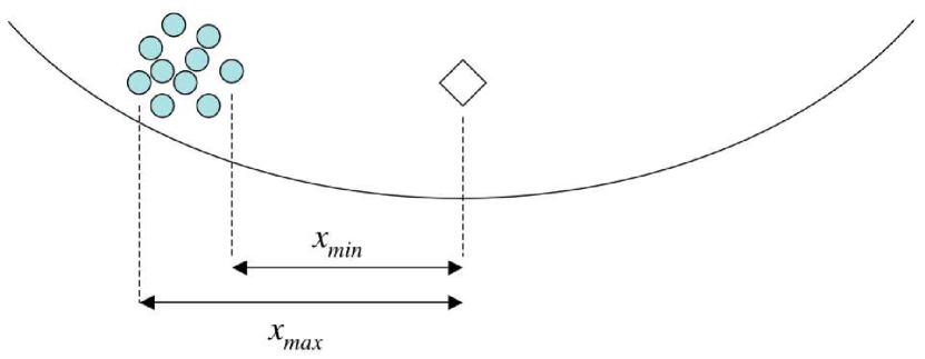
Figure 3: The difference in tether energy across a cluster configuration is given in terms of the maximum and minimum separations between an atom and its guide particle. The circles depict the argon atoms, while the diamond represents the position of all of the guides at the origin of the cell.

From the equilibrated molecular dynamics trajectory, we select, for disassembly, a set of ‘valid’ cluster configurations that satisfy the Stillinger cluster definition Stillinger (1963), but this can be quite difficult for the smaller clusters at 60 K. Tethering the atoms keeps them closer together and more likely to form valid configurations. We therefore choose a tethering strength that satisfies the condition on $\xi$, but also helps to produce sufficient valid cluster configurations. The initial value of the tethering force constant was taken to be $\kappa_{i}=0.01\,\mbox{kJ mol}^{-1}\mbox{\r{A}}^{-2}$, which gives $\xi\sim 0.6-0.9$ for the five sizes of argon cluster studied. Table 1 shows the duration of the equilibrated cluster trajectory, the number of valid cluster configurations identified from candidates selected at intervals of 100 ps from the equilibrated molecular dynamics trajectory, and the ratio $\xi$ characterising the suitability of the tethering force constant.

$i$	Duration/ns	Valid configurations	$\xi$
5	1000	152	0.604
10	250	411	0.745
15	225	1070	0.799
20	150	905	0.847
27	150	1020	0.922

Table 1: The duration of equilibrated cluster trajectories at 60 K, as well as the number of valid cluster configurations selected at each size. The ratio $\xi$ characterises the perturbation to the cluster energy due to the tether potentials.

Having obtained initial cluster configurations for the five sizes of cluster, the next stage is to disassemble them by a combination of guide particle motion and tether tightening. A range of separation times $t_{{\rm sep}}$ is explored, with the larger and more stable clusters expected to require longer disassembly processes in order to provide accurate estimates of the free energy change. As in the dimer calculations described in Appendix A, we use a tethering strength that strengthens in time according to Eqs. (24), with a final value of $\kappa_{f}=0.05\,\mbox{kJ mol}^{-1}\mbox{\r{A}}^{-2}$.

The terminal positions for the guide particles are chosen from a $3\times 3\times 3$ grid with spacing of $33.33\,\mbox{\r{A}}$. The largest cluster considered contains 27 argon atoms so after the process of disassembly, the tethered atoms move around each point on this grid. For smaller systems, the same grid of final guide positions is adopted, but employing only as many points as are necessary for the cluster in question. With initial guide positions at the origin and final positions defined in this way, it is straightforward to calculate the necessary drift velocities of the guide particles for a given separation time. Applying the Jarzynski procedure to the distribution of performed work then gives us the estimated free energy change $\Delta F$ associated with the disassembly of a cluster.

However, as mentioned previously, this free energy difference will only correspond to the disassembly of a tethered $i$-cluster, rather than of a freely translating, undistorted cluster. Furthermore, by necessity we obtain free energies of systems of distinguishable atoms in molecular dynamics, and we need to make an indistinguishability correction. An analysis of the thermodynamics is required in order to extract the excess free energy of an $i$-cluster from the free energy of disassembly, and the details are given in Appendix B. It turns out that we can write $F_{s}(i)=\sum_{k=1}^{5}f_{s}^{k}(i)$ with

$$f_{s}^{1}(i) = -\Delta F$$ (13)

$$f_{s}^{2}(i) = -ikT\ln\left(\rho_{vs}v_{{\rm HO}}\right)$$ (14)

$$f_{s}^{3}(i) = kT\ln\left(\rho_{vs}v_{c}\right)$$ (15)

$$f_{s}^{4}(i) = -\frac{3i\kappa_{i}}{10}\left(\frac{3iv_{l}}{4\pi}\right)^{2/3}$$ (16)

$$f_{s}^{5}(i) = kT\ln i!$$ (17)

In the first term the free energy of disassembly $\Delta F$ appears with a negative sign because it refers to the process of taking a cluster apart while $F_{s}$ is the free energy of interface formation. The $f_{s}^{2}$ term arises from relating the final state in the disassembly process, namely the separated harmonically bound particles, to the appropriate reference state of a saturated vapour. It represents the difference in free energy between the tethered particles, each effectively confined to a volume $v_{{\rm HO}}=\left(2\pi kT/\kappa_{f}\right)^{3/2}$, and particles in the saturated vapour phase with density $\rho_{vs}$ and volume per particle $1/\rho_{vs}$. The $f_{s}^{3}$ term is the entropy penalty associated with the initial tethering: the centre of mass of the cluster is effectively confined to a volume $v_{c}=\left(i\kappa_{i}/(2\pi kT)\right)^{-3/2}$ and needs to be referred to a situation where it is allowed, like a particle in saturated vapour, to explore a volume $1/\rho_{vs}$. The $f_{s}^{4}$ term is an approximate expression for the perturbation in the cluster energy due to the initial presence of the tethers, where $v_{l}=1/\rho_{l}$ is the volume per particle in the condensed phase. Finally, $f_{s}^{5}$ converts calculations derived from molecular dynamics with distinguishable particles into results relevant to a system of indistinguishable particles.

III.2 Results and discussion

A typical example of the work $W(t)$ performed over a disassembly trajectory of duration 20 ns for a 27-atom cluster is shown in Figure 4. The gradual rise in the work performed prior to about $5\mbox{ ns}$ represents an accumulation of tethering energy as the guide particles move away from their initial positions at the origin. After this time, atoms begin to leave the cluster, and less work is needed to move the corresponding guides. After about 7 ns, the work rate reduces significantly as the cluster disintegrates and the guide particles move towards their final positions.

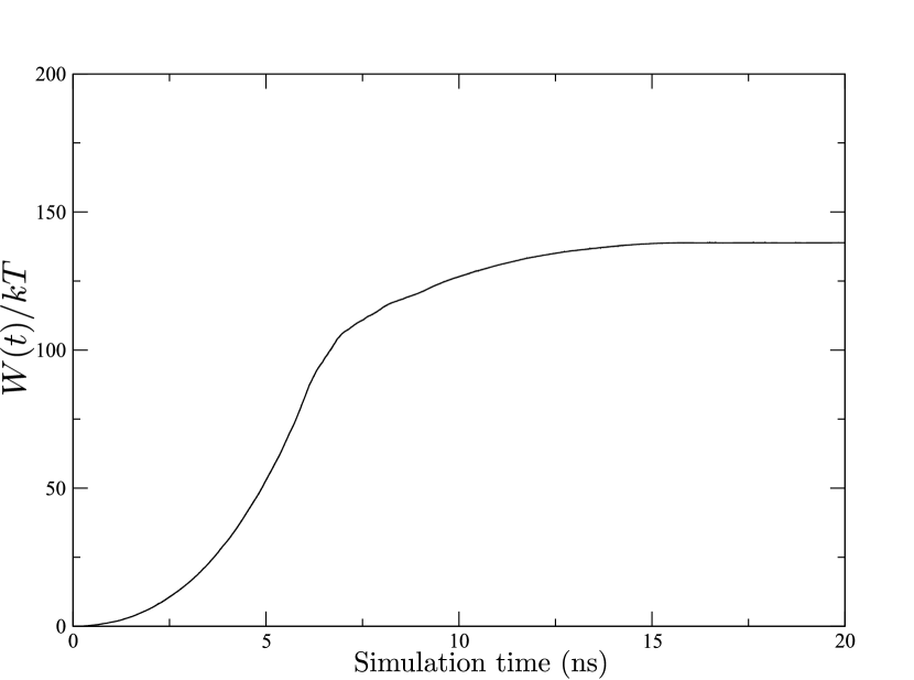
Figure 4: A typical history of the work performed for one realisation of the disassembly of a 27-atom argon cluster with a separation time of $20\,\mbox{ns}$.

Visual representations of the disassembly process (see Figure 5) provide further insight into the manner in which the clusters are pulled apart. The onset of cluster disassembly is signalled by the loss of one or two atoms from the cluster, perhaps only temporarily. The cluster soon after breaks into several smaller clusters, which eventually disintegrate into fragments or single atoms. It is rare to see a complete and sudden disintegration of a cluster, where all the constituent atoms disassemble together within a short space of time.

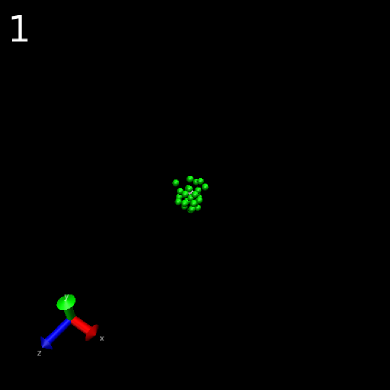
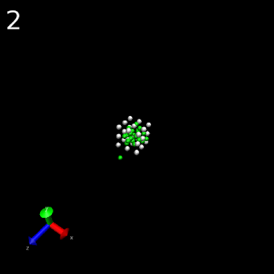
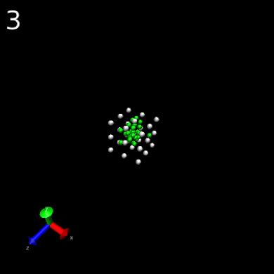
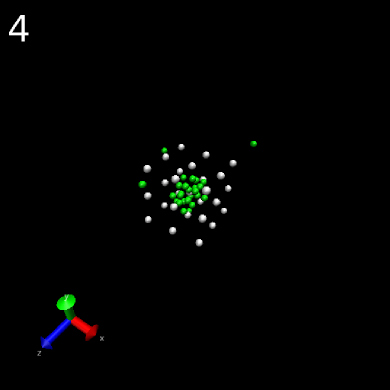
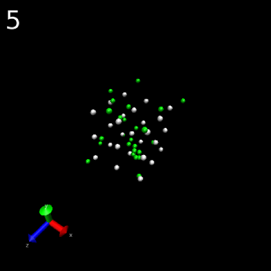
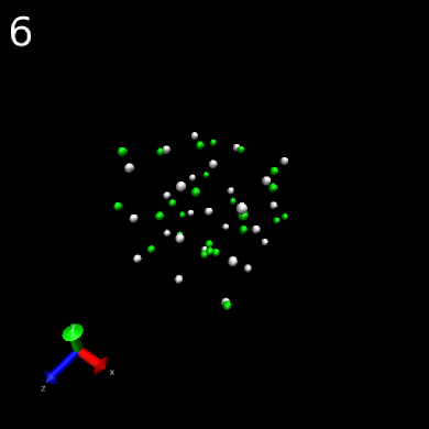
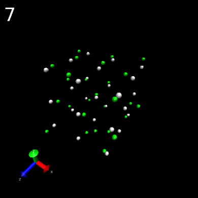
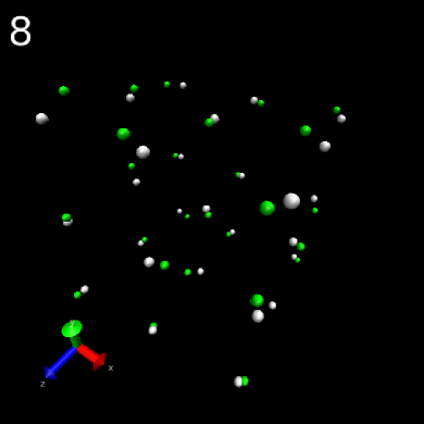
Figure 5: Illustration of the disassembly of a 27-atom argon cluster, with green spheres representing the argon atoms and lighter spheres the guide particles (helium atoms are not shown). In frame 1, all the guides lie at the origin of the cell. By frame 2, the guides have drifted far enough apart for a single argon atom to escape temporarily from the cluster before rejoining it in frame 3. In frame 4, several atoms have escaped, but remain in close proximity to the reduced cluster. A threshold is reached in frame 5, where many argon atoms break free to leave a fragment of about five atoms that also soon disintegrates as shown in frame 6. Shortly after, all of the atoms fall into motion about their partner guide particles which continue along steady paths away from one another (frames 7 and 8). The reader is encouraged to view movies of the disassembly provided in the Supplemental Material sup .

Figures 6 and 7 show distributions of the work performed in disassembling the 5-cluster and the 27-cluster, along with estimates of the free energy change, for separation times between 0.5 ns and 20 ns. As expected, the work distributions are broader for the processes that are most rapid (smallest $t_{{\rm sep}}^{-1}$) and hence least quasistatic in nature. Conversely, the work distributions become narrower, and lead to free energy changes that presumably provide the most accurate estimates of the true free energy change, as the rate of separation is reduced.

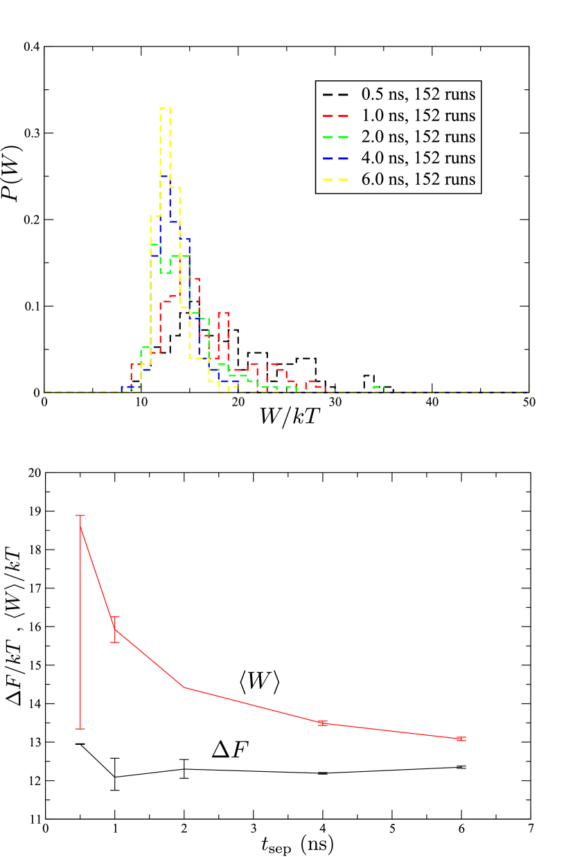
Figure 6: The distribution of work $W$ (top) for sets of disassembly trajectories for the 5-atom argon cluster, for a range of separation times. The lower plot shows the mean of the work $\langle W\rangle$ and the corresponding free energy differences $\Delta F$ calculated via the Jarzynski equality for each $t_{{\rm sep}}$.

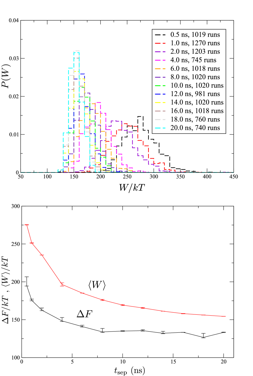
Figure 7: Plots similar to those shown in Figure 6 but for the 27-atom argon cluster.

The free energy change $\Delta F$ for the disassembly of each size of cluster at the slowest rate studied is shown in Table 2, along with the other contributions to the excess free energy $F_{s}$. We refer to a molecular dynamics study by Baidakov $et\,al.$ Baidakov et al. (2007) to provide values of the saturated vapour density $\rho_{vs}$ and liquid density $\rho_{l}=1/v_{l}$ of the argon-like Lennard-Jones fluid at a temperature of 60.31 K.

$i$	$t_{{\rm sep}}(\mathrm{ns)}$	$\langle W\rangle$	$\Delta F$	$f_{s}^{2}(i)$	$f_{s}^{3}(i)$	$f_{s}^{4}(i)$	$f_{s}^{5}(i)$	$F_{s}(i)$
5	6	13.08	12.35	38.94	-7.79	-0.41	4.79	23.18
10	8	34.06	30.80	77.88	-8.83	-1.32	15.10	52.03
15	12	62.75	53.87	116.81	-9.44	-2.59	27.90	78.82
20	16	97.37	84.07	155.75	-9.87	-4.18	42.33	99.97
27	20	154.41	133.28	210.27	-10.32	-6.90	64.56	124.33

Table 2: Results from the slowest set of disassembly simulations for each cluster size: the mean work $\langle W\rangle$, the free energy of disassembly $\Delta F$ and the other contributions to the excess free energy $F_{s}(i)$, all in units of $kT$.

Figure 8 shows our excess free energies $F_{s}(i)$ as a function of cluster size $i$. Statistical errors propagated from uncertainties in the free energy change $\Delta F$ are similar to the size of the symbols. We also include corresponding results from the Monte Carlo studies by Barrett and Knight Barrett and Knight (2008) and Merikanto $et\,al.$ Merikanto et al. (2006, 2007). Barrett and Knight employed a Lee-Barker-Abraham cluster definition Lee et al. (1973) while Merikanto $et\,al.$ adopted a Stillinger cluster criterion similar to ours. The Barrett and Knight calculations are represented here by $F_{s}^{{\rm BK}}(i)/kT=-\ln q_{i}-(i-1)\ln(\rho_{vs}\sigma_{{\rm ArAr}}^{3})$ with their fitting function $\ln q_{i}=10.5+9.91(i-1)-16.36(i^{2/3}-1)$, and the Merikanto $et\,al.$ values are derived from their Figure 1 in Merikanto et al. (2006), which we interpret as a plot of $F_{s}^{{\rm M}}(i)/kT-(i-1)\ln S$ with $S=20$. The results of these earlier studies are consistent with one another, as well as with the excess free energy suggested by the internally consistent classical theory (ICCT) $F_{s}^{{\rm ICCT}}(i)=\gamma\left(36\pi v_{l}^{2}\right)^{1/3}\left(i^{2/3}-1\right)$, constructed such that $F_{s}^{{\rm ICCT}}(1)=0$, where $\gamma$ is the surface tension of the planar liquid-vapour interface, again taken from Baidakov $et\,al.$ Baidakov et al. (2007). It is clear from Figure 8 that the calculations presented in this study are consistent with the previous Monte Carlo results. This is satisfactory support for the disassembly approach that we have developed. We note that all three are reasonably well represented by the ICCT model, which is somewhat surprising.

Note that the construction of a traditional plot of the nucleation barrier such as Figure 1 would require us to subtract a term $ikT\ln S$ from the excess free energies in Figure 8. Inserting a supersaturation of $30$ would then yield a critical size of about 20, for example.

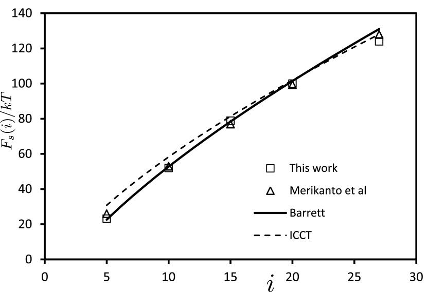
Figure 8: Excess free energies for argon-like Lennard-Jones clusters obtained from disassembly at 60 K are shown as squares and compared with values obtained in Monte Carlo studies by Barrett and Knight Barrett and Knight (2008) at $59.88\,\mbox{K}$ (solid line) and Merikanto $et\,al.$ Merikanto et al. (2006, 2007) at $60.18\,\mbox{K}$ (triangles). Also shown is the prediction from internally consistent classical nucleation theory for a temperature of $60.31\,\mbox{K}$ (dashed line).

IV Conclusions

We have developed a method of guided cluster disassembly in molecular dynamics, capable of extracting the excess free energy associated with the formation of a molecular cluster from the saturated vapour phase. This property is often regarded as a surface term and it plays a central role in kinetic and thermodynamic models of the process of droplet nucleation.

After exploring some aspects of the method by separating a dimer, the technique was applied to the controlled disassembly of Lennard-Jones argon clusters between 5 and 27 atoms in size. The extracted free energy of disassembly has been related to the excess free energy of the cluster through an analysis of the statistical mechanics of free and tethered clusters. Our calculations for clusters of various sizes are consistent with previous studies by Barrett and Knight Barrett and Knight (2008) and Merikanto et al. Merikanto et al. (2006, 2007), both of which require the evaluation of a sequence of free energy differences between monomer and dimer, dimer and trimer, etc. A Lennard-Jones microscopic model of argon, within the standard kinetic and thermodynamic framework of nucleation theory, cannot account for the experimental argon nucleation data of Iland et al. Iland et al. (2007), but we do not speculate here about this disparity.

The approach should be contrasted with methods of free energy estimation based on thermodynamic integration. In those methods, the strength of the interparticle interactions is evolved over a sequence of equilibrium calculations. Our approach also involves the evolution of a Hamiltonian, but it is the tether potentials that change with time, not the interparticle interactions. Furthermore, we evolve by nonequilibrium molecular dynamics rather than studying a sequence of equilibrium ensembles, and we are only required to apply a cluster definition when selecting the initial configurations, not during the evolution.

We believe that our process of mechanical disassembly offers an intuitive understanding of the meaning of the work of formation that plays such a central role in nucleation theory. We suggest that a direct evaluation of this quantity is preferable to an approach based on summing the free energy changes associated with the addition of single molecules to a cluster, on the grounds that we avoid the possible compounding of statistical errors. The computational costs of our current study of argon clusters have been higher than those of more traditional methods such as grand canonical Monte Carlo Merikanto et al. (2007), for the same level of accuracy, largely because of our exploration of different protocols and our use of an explicit helium thermostat, but these can be reduced with further development. A particularly powerful variant of the disassembly scheme is to separate a cluster into two subclusters under similar mechanical guidance, in order to relate the distribution of work performed to a free energy of ‘mitosis’, essentially a difference in excess free energies between the initial cluster and the two final subclusters. Such comparisons would be unfeasible to perform in Monte Carlo. The calculations are not onerous and an evaluation of the excess free energy of clusters of up to 128 water molecules is to be reported Lau . Furthermore, the explicit thermostat can be replaced by an implicit scheme. With such tools, and guided by the experience developed in the current investigation of argon, we intend to carry out studies of clusters of water, acids and organic molecules, species that are particularly relevant to the process of aerosol nucleation in the atmosphere.

Appendix A Argon dimer separation

We test the feasibility of the approach using two protocols of controlled dimer separation. First, the guide particles are made to drift apart with the tether strengths held constant, and then we allow the tethers to tighten over the course of the process. We determine the manner of dimer separation that leads to an accurate estimate of the free energy change.

We start by evaluating the free energy of a tethered dimer of argon-like atoms analytically. Particles are distinguishable in molecular dynamics simulations since they carry labels, so we take this into account in the analysis. The initial Hamiltonian of the dimer system is

$$H_{i}^{{\rm dimer}}=\, \frac{\boldsymbol{p}_{1}^{2}}{2m}+\frac{\boldsymbol{p}_{2}^{2}}{2m}+\frac{1}{2}\kappa_{i}\left(\boldsymbol{x}_{1}-\mathbf{X}_{1}\right)^{2}$$ (18)

$$+\, \frac{1}{2}\kappa_{i}\left(\boldsymbol{x}_{2}-\mathbf{X}_{2}\right)^{2}+\Phi\left(|\boldsymbol{x}_{1}-\boldsymbol{x}_{2}|\right),$$

where $m$ is the argon mass, and $\Phi(|\boldsymbol{x}_{1}-\boldsymbol{x}_{2}|)$ is a pairwise interaction potential. When the guide particles both lie at the origin $(\mathbf{X}_{1}=\mathbf{X}_{2}=0)$, the initial partition function is

$$Z_{i}^{{\rm dimer}}=\frac{1}{h^{6}}\int\exp\left(-\frac{p_{1}^{2}+p_{2}^{2}}{2mkT}\right)d\boldsymbol{p}_{1}d\boldsymbol{p}_{2}$$ (19)

$$\times\int\exp\left(-\kappa_{i}\frac{x_{1}^{2}+x_{2}^{2}}{2kT}\right)\exp\left(-\frac{\Phi\left(|\boldsymbol{x}_{1}-\boldsymbol{x}_{2}|\right)}{kT}\right)d\boldsymbol{x}_{1}d\boldsymbol{x}_{2},$$

noting that there is no correction factor of one half since the atoms are distinguishable. Substituting $\boldsymbol{r}=\boldsymbol{x}_{1}-\boldsymbol{x}_{2}$ and $\boldsymbol{R}=\boldsymbol{x}_{1}+\boldsymbol{x}_{2}$, the partition function $Z_{i}^{{\rm dimer}}$ becomes

$$\frac{1}{\lambda_{{\rm th}}^{6}}\int\frac{1}{8}\exp\left(-\kappa_{i}\frac{x_{1}^{2}+x_{2}^{2}}{2kT}\right)\exp\left(-\frac{\Phi\left(|\boldsymbol{x}_{1}-\boldsymbol{x}_{2}|\right)}{kT}\right)d\boldsymbol{r}d\boldsymbol{R}$$

$$=\frac{1}{\lambda_{{\rm th}}^{6}}\frac{\pi}{2}\int\exp\left(-\kappa_{i}\frac{R^{2}+r^{2}}{4kT}\right)\exp\left(-\frac{\Phi\left(r\right)}{kT}\right)r^{2}drd\boldsymbol{R}$$

$$=\frac{1}{\lambda_{{\rm th}}^{6}}\frac{\pi}{2}\left(\frac{4\pi kT}{\kappa_{i}}\right)^{\frac{3}{2}}\int_{0}^{r_{c}}r^{2}\exp\left(-\frac{\kappa_{i}r^{2}+4\Phi(r)}{4kT}\right)dr,$$ (20)

where $\lambda_{{\rm th}}=h/(2\pi mkT)^{1/2}$ is the thermal de Broglie wavelength. We have imposed an upper limit $r_{c}$ on the separation between the two atoms, corresponding to a definition of what we mean by a dimer.

For the final state in which the two argon atoms are tethered to respective guide particles that are far apart, the Hamiltonian is simply that in Eq. (18) without the interaction term, and with a final tether strength $\kappa_{f}$. The corresponding final partition function is

$$Z_{f}^{{\rm dimer}}=\frac{1}{h^{6}}\int\exp\left(-\frac{p_{1}^{2}+p_{2}^{2}}{2mkT}\right)d\boldsymbol{p}_{1}d\boldsymbol{p}_{2}$$ (21)

$$\times\int\exp\left(-\kappa_{f}\frac{x_{1}^{2}+x_{2}^{2}}{2kT}\right)d\boldsymbol{x}_{1}d\boldsymbol{x}_{2}=\frac{1}{\lambda_{{\rm th}}^{6}}\left(\frac{2\pi kT}{\kappa_{f}}\right)^{3}.$$

The free energy change in separating a dimer of tethered atoms can therefore be expressed as

$$\Delta F=kT\ln\left(Z_{i}^{{\rm dimer}}/Z_{f}^{{\rm dimer}}\right)$$ (22)

$$=kT\ln\left[\left(\frac{\kappa_{f}^{2}}{\kappa_{i}kT}\right)^{\frac{3}{2}}\int_{0}^{r_{c}}\frac{r^{2}}{2\sqrt{\pi}}\exp\left(-\frac{\kappa_{i}r^{2}+4\Phi(r)}{4kT}\right)dr\right],$$

which can be evaluated numerically. The parameter $r_{c}$ is the Stillinger radius used to identify a dimer configuration in the equilibrated molecular dynamics simulation, to which we now turn.

We place two argon-like particles within a periodic cell with edge length 50 Å, each tethered to guide particles through a harmonic interaction $\frac{1}{2}\kappa(t)r^{2}$, where $r$ is the separation between the argon atom and its guide, and $\kappa(t)$ is the tethering force constant. The argon atoms are thermalised through interaction with a gas of 100 helium-like atoms kept at constant temperature using a Nosé-Hoover thermostat. Conventional masses of 39.85 and 4.003 amu for the argon and helium-like particles are adopted, while the guide particles are assigned a vastly greater mass of $4\times 10^{12}$ amu. Interaction potentials are specified by

$$\Phi\left(r_{jk}\right)=4\epsilon_{jk}\left[\left(\frac{\sigma_{jk}}{r_{jk}}\right)^{12}-\left(\frac{\sigma_{jk}}{r_{jk}}\right)^{6}\right],$$ (23)

with parameters shown in Table 3, though it should be noted that only the repulsive part of the interaction between argon and helium is employed in order to prevent any binding between the two. Simulations are performed at a temperature of 15 K such that dimers are long-lived and a sufficient number of configurations satisfying the separation criterion $r\leq r_{c}=1.5\sigma_{{\rm ArAr}}$ can be obtained from the equilibrated trajectory. With a constant tethering force constant of $0.05\,\text{kJ mol}^{-1}\text{\r{A}}^{-2}$, we generate an equilibrated molecular dynamics trajectory of duration 100 ns and choose $10^{3}$ dimer configurations for use as starting points for the separation process.

$j$	$k$	$\epsilon_{jk}$ / $\mbox{kJ mol}^{-1}$	$\sigma_{jk}$ / Å
Ar	Ar	0.995581	3.405
He	He	0.084311	2.600
Ar	He	0.289721	3.000

Table 3: Parameters for the Lennard-Jones potentials, where $j$ and $k$ are the atomic labels, $\epsilon_{jk}$ is the depth of the potential well, and $\sigma_{jk}$ is the range parameter Hirschfelder et al. (1964).

A.0.1 Guiding at constant tether strength

One of the guide particles drifts from the origin to a corner of the cubic simulation cell over a separation time $t_{{\rm sep}}$ while the other remains stationary (see Figure 9). We choose $t_{{\rm sep}}$ to be 1, 2 or 4 ns and the velocity of the moving guide particle (labelled 1) is given by $\mathbf{V}_{1}=[\mathbf{X}_{1}(t=t_{{\rm sep}})-\mathbf{X}_{1}(t=0)]/t_{{\rm sep}}$.

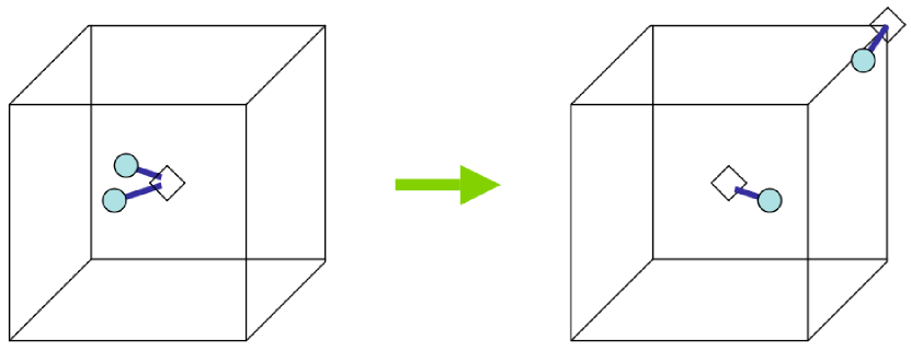
Figure 9: Illustration of the dimer separation process. Both guide particles (diamonds) are initially at the origin, but one is made to drift towards a corner of the simulation cell.

For initial and final tethering force constants of $0.05\,\text{kJ mol}^{-1}\text{\r{A}}^{-2}$, the expected free energy change in separating the dimer is $5.716\,kT$ according to Eq. (22). Distributions of the work done for each rate of dimer separation are shown in Figure 10, and the corresponding estimates of the free energy change obtained from the Jarzynski equality are compared with the expected value in the lower part of Figure 11. A longer separation time leads to a better estimate of the free energy change since the process is then closer to being quasistatic.

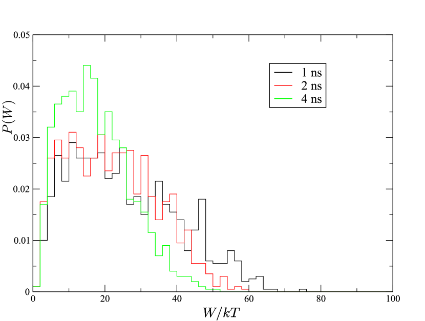
Figure 10: Distributions of the work done in the disassembly of a dimer for separation times $t_{{\rm sep}}$ of 1, 2 and 4 ns.

Figure 11: Convergence of the Jarzynski-estimated free energy change toward the expected value (dashed line) as the dimer separation rate is decreased, while keeping the tethering strength constant (lower set) and when the tethers are tightened (upper set).

A.0.2 Guiding with tether tightening

We now elaborate the process by tightening the tethers during guide drift according to

$$\kappa(t) = \kappa_{i}\quad\text{for}\;t\leq t_{i}$$ (24)

$$= \kappa_{i}+\frac{\kappa_{f}-\kappa_{i}}{2}\left[1-\cos\left(\pi\frac{t-t_{i}}{t_{s}-t_{i}}\right)\right]\;\text{for}\;t_{i}<t\leq t_{s}$$

$$= \kappa_{f}\quad\text{for}\;t>t_{s},$$

where $t_{i}$ is the time at which the force constant begins to change, and $t_{s}$ is the time at which it reaches its final value. Once again starting with dimer configurations and an initial tethering force constant of $0.05\,\text{kJ mol}^{-1}\text{\r{A}}^{-2}$ at 15 K, three dimer separation times are investigated, during which the force constant rises by a factor of two. The times $t_{i}$ and $t_{s}$ are specified as 20% and 80% of the total separation time. The expected free energy change associated with dimer separation is $7.795\,kT$ according to Eq. (22). It can be seen from the upper part of Figure 11 that all three separation rates give acceptable estimates of the free energy change. Furthermore, the greater compatibility between the distributions of the work performed at different separation rates shown in Figure 12, compared with those in the simulations with constant tether strength, suggests that a protocol where the tethers tighten while the guide particles drift apart is more effective. Intuitively, the separation is then conducted more firmly, and with less dissipation.

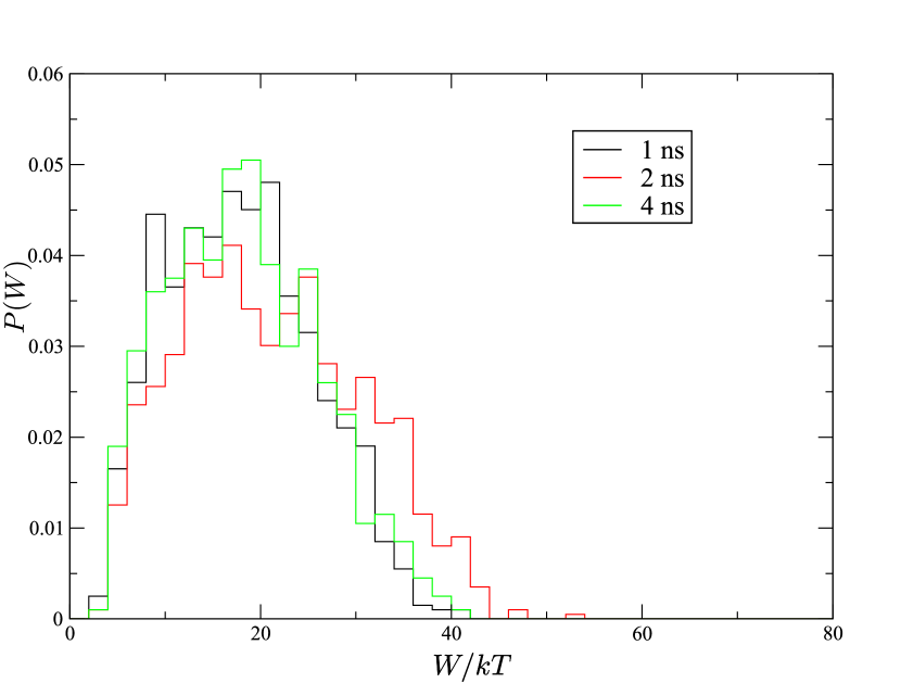
Figure 12: Distributions of the work of dimer disassembly where the atoms are guided apart and the tethers tightened for three different separation times.

Appendix B Analysis of cluster free energies

B.1 Free and tethered clusters

The canonical partition function $Z_{F}=\exp\left(-F_{F}/kT\right)$ for an untethered, or ‘free’ cluster of $i$ indistinguishable particles governed by a Hamiltonian $H$ composed of kinetic energy terms and pairwise interactions is given by

$$Z_{F} = \frac{1}{i!h^{3i}}\int\prod\limits_{j=1}^{i}d\boldsymbol{x}_{j}d\boldsymbol{p}_{j}\exp\left[-H\left(\left\{\boldsymbol{x}_{k}\right\}\right)/kT\right],$$ (25)

where $F_{F}$ is the associated free energy. For a cluster tethered to the origin, the Hamiltonian will include an additional set of harmonic potentials, such that the partition function is

$$Z_{T} = \exp\left(-F_{T}/kT\right)=\frac{1}{i!h^{3i}}\int\prod\limits_{j=1}^{i}d\boldsymbol{x}_{j}d\boldsymbol{p}_{j}$$ (26)

$$\times \exp\left[-\left(H\left(\left\{\boldsymbol{x}_{k}\right\}\right)+\sum\limits_{j=1}^{i}\frac{1}{2}\kappa_{i}x_{j}^{2}\right)/kT\right],$$

where $F_{T}$ is the free energy of the tethered cluster, and $\kappa_{i}$ is the initial tethering force constant.

We insert a factor of unity in the form $1=\int\delta\left(\frac{1}{i}\sum_{j=1}^{i}\boldsymbol{x}_{j}-\boldsymbol{x}_{c}\right)d\boldsymbol{x}_{c}$ into Eqs. (25) and (26), and transform to particle coordinates with respect to the cluster centre of mass $\boldsymbol{x}_{c}$, namely $\boldsymbol{x}_{j}^{\prime}=\boldsymbol{x}_{j}-\boldsymbol{x}_{c}$. The partition function for a free cluster becomes

$$Z_{F} = \frac{1}{i!h^{3i}}\int\prod\limits_{j=1}^{i}d\boldsymbol{x}_{j}^{\prime}d\boldsymbol{p}_{j}d\boldsymbol{x}_{c}\exp\left[-H\left(\left\{\boldsymbol{x}_{k}^{\prime}\right\}\right)/kT\right]$$ (27)

$$\times\delta\left(\frac{1}{i}\sum\limits_{j=1}^{i}\boldsymbol{x}_{j}^{\prime}\right)$$

$$= \frac{V}{i!h^{3i}}\int\prod\limits_{j=1}^{i}d\boldsymbol{x}_{j}^{\prime}d\boldsymbol{p}_{j}\exp\left[-H\left(\left\{\boldsymbol{x}_{k}^{\prime}\right\}\right)/kT\right]$$

$$\times\delta\left(\frac{1}{i}\sum\limits_{j=1}^{i}\boldsymbol{x}_{j}^{\prime}\right)=VZ_{F}^{c},$$

where $V$ is the system volume and $Z_{F}^{c}$ is the partition function for a cluster whose centre of mass is fixed at the origin. It should be noted that since the Hamiltonian contains pairwise interactions, it may be rewritten as $H(\{\boldsymbol{x}_{k}\})=H(\{\boldsymbol{x}_{k}^{\prime}\})$ after the change of variables.

Similarly, the partition function for a tethered cluster can be rewritten as

$$Z_{T}=\frac{1}{i!h^{3i}}\int\prod\limits_{j=1}^{i}d\boldsymbol{x}_{j}^{\prime}d\boldsymbol{p}_{j}d\boldsymbol{x}_{c}\delta\left(\frac{1}{i}\sum\limits_{j=1}^{i}\boldsymbol{x}_{j}^{\prime}\right)$$ (28)

$$\times\exp\left[-\left(H\left(\left\{\boldsymbol{x}_{k}^{\prime}\right\}\right)+\sum\limits_{j=1}^{i}\frac{1}{2}\kappa_{i}x_{j}^{2}\right)/kT\right].$$

The second term in the exponent of Eq. (28) may be simplified using the constraint $\sum_{j=1}^{i}\boldsymbol{x}_{j}^{\prime}=0$ and it follows that $\sum_{j=1}^{i}x_{j}^{2}=\sum_{j=1}^{i}x_{j}^{\prime 2}+ix_{c}^{2}$, giving

$$Z_{T}=\frac{1}{i!h^{3i}}\int\prod\limits_{j=1}^{i}d\boldsymbol{x}_{j}^{\prime}d\boldsymbol{p}_{j}d\boldsymbol{x}_{c}\exp\left[-\frac{1}{2}\kappa_{i}ix_{c}^{2}/kT\right]$$

$$\times\exp\left[-\left(H\left(\left\{\boldsymbol{x}_{k}^{\prime}\right\}\right)+\frac{1}{2}\kappa_{i}\sum\limits_{j=1}^{i}x_{j}^{\prime 2}\right)/kT\right]\delta\left(\frac{1}{i}\sum\limits_{j=1}^{i}\boldsymbol{x}_{j}^{\prime}\right)$$

$$=\left(\frac{2\pi kT}{i\kappa_{i}}\right)^{\frac{3}{2}}\frac{1}{i!h^{3i}}\int\prod\limits_{j=1}^{i}d\boldsymbol{x}_{j}^{\prime}d\boldsymbol{p}_{j}\exp\left[-H\left(\left\{\boldsymbol{x}_{k}^{\prime}\right\}\right)/kT\right]$$

$$\times\exp\left[-\frac{1}{2}\kappa_{i}\sum\limits_{j=1}^{i}x_{j}^{\prime 2}/kT\right]\delta\left(\frac{1}{i}\sum\limits_{j=1}^{i}\boldsymbol{x}_{j}^{\prime}\right)$$

$$=\left(\frac{2\pi kT}{i\kappa_{i}}\right)^{\frac{3}{2}}Z_{T}^{c},$$ (29)

where $Z_{T}^{c}$ is the partition function of a cluster constrained to have its centre of mass at the origin as well as having its constituent particles tethered to the origin by a harmonic potential.

Next, we employ the Gibbs-Bogoliubov approach Hansen and McDonald (1986); Ishihara (1968) to compare the free energies $F_{F}^{c}$ and $F_{T}^{c}$ of systems with Hamiltonians $H_{0}$ and Hamiltonian $H_{0}+U$, defined by $\exp\left(-F_{F}^{c}/kT\right)=\int d\Gamma\exp\left[-H_{0}/kT\right]$ and $\exp\left(-F_{T}^{c}/kT\right)=\int d\Gamma\exp\left[-\left(H_{0}+U\right)/kT\right]$, where $\Gamma$ represents the configuration of a system, and $d\Gamma$ is proportional to the phase space volume element $\Pi_{j}d\boldsymbol{x}_{j}^{\prime}d\boldsymbol{p}_{j}$. In the context of the tethered cluster described by Eq. (29), $U$ represents the term $\frac{1}{2}\kappa_{i}\sum_{j=1}^{i}x_{j}^{\prime 2}$, while $H_{0}$ is the untethered Hamiltonian $H\left(\left\{\boldsymbol{x}_{k}^{\prime}\right\}\right)$ modified by the delta function constraint. $F_{T}^{c}$ is therefore the free energy of a tethered cluster with its centre of mass further constrained to lie at the origin, and is equal to $-kT\ln Z_{T}^{c}$. A similar relationship exists between $F_{F}^{c}$, the free energy of an untethered cluster with fixed centre of mass, and $Z_{F}^{c}$.

The free energies $F_{F}^{c}$ and $F_{T}^{c}$ may be related through

$$\!\!\!\exp\left(-F_{T}^{c}/kT\right) = \frac{\int d\Gamma\exp\left(-H_{0}/kT\right)\exp\left(-U/kT\right)}{\int d\Gamma\exp\left(-H_{0}/kT\right)}$$ (30)

$$\times\int d\Gamma\exp\left(-H_{0}/kT\right)$$

$$= \left<\exp\left(-U/kT\right)\right>_{0}\exp\left(-F_{F}^{c}/kT\right),$$

where angle brackets represent an average in the statistical ensemble corresponding to $H_{0}$. For small $\left<U/kT\right>_{0}$, we can write $\left<\exp\left(-U/kT\right)\right>_{0}\simeq\exp\left(-\left<U\right>_{0}/kT\right)$, and hence

$$\exp\left(-F_{T}^{c}/kT\right) \simeq \exp\left[\left(-F_{F}^{c}-\left<U\right>_{0}\right)/kT\right],$$ (31)

with $\langle U\rangle_{0}$ given by

$$\langle U\rangle_{0}=\frac{\int d\Gamma U\left(\left\{\boldsymbol{x}_{k}^{\prime}\right\}\right)\exp\left(-H_{0}/kT\right)}{\int d\Gamma\exp\left(-H_{0}/kT\right)}.$$ (32)

$U(\{\boldsymbol{x}_{k}^{\prime}\})$ is a sum of single-particle harmonic potentials of the form $U_{{\rm HO}}(\boldsymbol{x}_{k}^{\prime})=\frac{1}{2}\kappa_{i}x_{k}^{\prime 2}$, so Eq. (32) can be written as

$$\!\!\!\!\!\!\langle U\rangle_{0} = \frac{\sum_{k=1}^{i}\int d\Gamma U_{{\rm HO}}\left(\boldsymbol{x}_{k}^{\prime}\right)\exp\left(-H_{0}/kT\right)}{\int d\Gamma\exp\left(-H_{0}/kT\right)}$$ (33)

$$= i\frac{\int d\Gamma U_{{\rm HO}}\left(\boldsymbol{x}_{k}^{\prime}\right)\exp\left(-H_{0}/kT\right)}{\int d\Gamma\exp\left(-H_{0}/kT\right)}=i\langle U_{{\rm HO}}\rangle_{0}.$$

We next introduce the spatial density profile of a single particle (labelled $k$ without loss of generality) in a cluster constrained to have its centre of mass at the origin but not tethered, namely

$$\rho_{0}(\boldsymbol{y})=\frac{\int d\Gamma\exp\left(-H_{0}/kT\right)\delta(\boldsymbol{x}_{k}^{\prime}-\boldsymbol{y})}{\int d\Gamma\exp\left(-H_{0}/kT\right)},$$ (34)

with $\int\rho_{0}(\boldsymbol{y})d\boldsymbol{y}=1$. We can write

$$\left<U_{{\rm HO}}\right>_{0}=\int\rho_{0}(\boldsymbol{y})U_{{\rm HO}}(\boldsymbol{y})d\boldsymbol{y},$$ (35)

which represents the average tethering energy of a particle that is spatially distributed according to the density $\rho_{0}(\boldsymbol{y})$. The condition that the tether potential makes a relatively small contribution to the mean energy of the cluster is $\langle U_{{\rm HO}}\rangle_{0}=\frac{1}{2}\kappa_{i}\int\rho_{0}(\boldsymbol{y})y^{2}d\boldsymbol{y}\ll kT$, in which case the approximations involved in the Gibbs-Bogoliubov approach are acceptable and the initial tethering potential weak enough that the cluster is only slightly distorted in comparison with a free cluster. Thus we write

$$Z_{T}^{c}=\exp\left(-F_{T}^{c}/kT\right)\simeq\exp\left[\left(-F_{F}^{c}-i\left<U_{{\rm HO}}\right>_{0}\right)/kT\right].$$ (36)

Eq. (29) can then be written as

$$Z_{T}=\left(\frac{2\pi kT}{i\kappa_{i}}\right)^{\frac{3}{2}}\frac{1}{i!h^{3i}}\int\prod_{j=1}^{i}d\boldsymbol{x}_{j}^{\prime}d\boldsymbol{p}_{j}\exp\left[-H\left(\left\{\boldsymbol{x}_{k}^{\prime}\right\}\right)/kT\right]$$

$$\times\exp\left[-i\int\rho_{0}\left(\boldsymbol{y}\right)\kappa_{i}y^{2}d\boldsymbol{y}/2kT\right]\delta\left(\frac{1}{i}\sum_{j=1}^{i}\boldsymbol{x}_{j}^{\prime}\right),$$ (37)

such that the relationship between the partition function of a tethered cluster, and the partition function of a free cluster with a constrained centre of mass $Z_{F}^{c},$ is

$$Z_{T}=Z_{F}^{c}\left(\frac{2\pi kT}{i\kappa_{i}}\right)^{\frac{3}{2}}\exp\left[-i\int\rho_{0}\left(\boldsymbol{y}\right)\kappa_{i}y^{2}d\boldsymbol{y}/2kT\right].$$ (38)

Combining Eqs. (27) and (38) then gives

$$\!\!\!\!\!\!\!\!\!\!\!\!\!\ln Z_{T} = \ln\!\left[\frac{Z_{F}}{V}\left(\frac{2\pi kT}{i\kappa_{i}}\right)^{\frac{3}{2}}\right]-\frac{i\kappa_{i}}{2kT}\int\rho_{0}(\boldsymbol{y})y^{2}d\boldsymbol{y},$$ (39)

or

$$F_{F}-F_{T}=-kT\ln\left[\rho_{c}\left(0\right)V\right]-\frac{i\kappa_{i}}{2}\int\rho_{0}(\boldsymbol{y})y^{2}d\boldsymbol{y},$$ (40)

where $\left(i\kappa_{i}/2\pi kT\right)^{3/2}$ has been replaced by a function $\rho_{c}(0)$, representing the probability density that the centre of mass of the tethered cluster lies at the origin. This equivalence can be demonstrated by deriving the distribution of the cluster centre of mass, through considering a single particle with mass $M=im$ and coordinates $\boldsymbol{x}_{c}$ and $\boldsymbol{p}_{c}$ residing in a potential $i\kappa_{i}x_{c}^{2}/2$. The positional probability density at $\boldsymbol{z}$ is

$$\rho_{c}(\boldsymbol{z}) = \frac{\int d\boldsymbol{x}_{c}d\boldsymbol{p}_{c}\exp\left(-\frac{i\kappa_{i}x_{c}^{2}}{2kT}-\frac{p_{c}^{2}}{2MkT}\right)\delta\left(\boldsymbol{x}_{c}-\boldsymbol{z}\right)}{\int d\boldsymbol{x}_{c}d\boldsymbol{p}_{c}\exp\left(-\frac{i\kappa_{i}x_{c}^{2}}{2kT}-\frac{p_{c}^{2}}{2MkT}\right)}$$ (41)

$$= \left(\frac{i\kappa_{i}}{2\pi kT}\right)^{3/2}\exp\left(-\frac{i\kappa_{i}z^{2}}{2kT}\right),$$

such that $\rho_{c}(0)=\left(i\kappa_{i}/(2\pi kT)\right)^{3/2}$.

The purpose of the substitution is that the first term on the right hand side in Eq. (40) may be interpreted as two competing contributions to the free energy difference $F_{F}-F_{T}$. We write

$$-kT\ln\left[\rho_{c}\left(0\right)V\right]=-T\left[-k\ln\left(\frac{1}{\rho_{c}(0)}\right)+k\ln V\right],$$ (42)

such that the first term corresponds to the removal of the entropic contribution to free energy associated with the freedom of motion of the cluster centre of mass within a constrained volume $1/\rho_{c}(0)$, brought about by the tethers, and the second term represents the addition of entropic free energy corresponding to the freedom of motion in volume $V$. Finally, the second term in Eq. (40) is an estimate of the removal of tethering potential energy when relating a tethered to a free cluster.

B.2 Excess free energy from the free energy of disassembly

We now establish the relationship between the free energy of a free cluster to the cluster work of formation defined as $\phi\left(i\right)=\Omega_{s}(i)-ikT\ln S$, where $\Omega_{s}(i)=F_{F}(i)-i\mu_{s}$ is the grand potential of a free cluster of $i$ particles in an environment at chemical potential $\mu_{s}$ for which the bulk condensed and vapour phases coexist. The excess free energy (difference) of the cluster is therefore

$$F_{s}\left(i\right) =\phi\left(i\right)-\phi(1)+\left(i-1\right)kT\ln S$$

$$=F_{F}\left(i\right)-F\left(1\right)-\left(i-1\right)\mu_{s},$$ (43)

having used Eq. (7).

Assuming the vapour is ideal, the coexistence chemical potential $\mu_{s}$ and the monomer Helmholtz free energy $F(1)$ are simply $\mu_{s}=kT\ln(\rho_{vs}\Lambda)$ and $F(1)=-kT\ln(V/\Lambda)$, respectively, where $\rho_{vs}$ is the particle density in a saturated vapour and $\Lambda=\lambda_{{\rm th}}^{3}$ with $\lambda_{{\rm th}}=h/(2\pi mkT)^{1/2}$. The excess free energy $F_{s}(i)$ can now be expressed as

$$F_{s}(i) = F_{F}+kT\ln\left(V/\Lambda\right)-\left(i-1\right)kT\ln\left(\rho_{vs}\Lambda\right)$$ (44)

$$= F_{T}-kT\ln\left[\rho_{c}\left(0\right)V\right]-\frac{i\kappa_{i}}{2}\int\rho_{0}\left(\boldsymbol{y}\right)y^{2}d\boldsymbol{y}$$

$$+kT\ln\left(V/\Lambda\right)-\left(i-1\right)kT\ln\left(\rho_{vs}\Lambda\right).$$

Now we consider the free energy change associated with the process of cluster disassembly. The difference in free energy between separated constituent particles each tethered to a guide particle, and a tethered cluster, is $\delta F=F_{f}-F_{T}$, where $F_{f}=-3ikT\ln\left(kT/\hbar\omega_{f}\right)$ is the free energy of $i$ harmonic oscillators in three dimensions, where the angular frequency $\omega_{f}=\left(\kappa_{f}/m\right)^{1/2}$ of the oscillators is related to the final value of the tethering force constant $\kappa_{f}$ .

It should be recognised, however, that the quantity $\delta F$ is not the free energy difference extracted from the molecular dynamics simulations of cluster disassembly. Molecular dynamics simulations always involve distinguishable particles, since they are assigned labels, and $\delta F$ is a difference between the free energy of $i$ indistinguishable particles in a cluster, and $i$ particles that are distinguishable through having been physically separated to regions around their final tether points.

The free energy difference that is extracted in our procedure is actually $\Delta F=F_{f}-F_{T}^{{\rm dist}}$, where the superscript in $F_{T}^{{\rm dist}}$ reminds us that it is the free energy of a tethered cluster of distinguishable particles. But we can relate the partition function of such a cluster to the partition function $Z_{T}$ for indistinguishable particles by the usual classical procedure, namely $Z_{T}^{{\rm dist}}=i!Z_{T}$, and since $F_{T}^{{\rm dist}}=-kT\ln Z_{T}^{{\rm dist}}=-kT\ln Z_{T}-kT\ln i!=F_{T}-kT\ln i!$ we have

$$\Delta F=F_{f}-F_{T}+kT\ln i!=\delta F+kT\ln i!,$$ (45)

such that $F_{T}=F_{f}-\delta F=F_{f}-\Delta F+kT\ln i!$. Substituting into Eq. (44) then gives

$$F_{s}(i) =-\Delta F-ikT\ln\left(\rho_{vs}v_{{\rm HO}}\right)+kT\ln i!$$

$$-kT\ln\left(\frac{\rho_{c}(0)}{\rho_{vs}}\right)-\frac{i\kappa_{i}}{2}\int\rho_{0}\left(\boldsymbol{y}\right)y^{2}d\boldsymbol{y},$$ (46)

where $v_{{\rm HO}}=\left(2\pi kT/\kappa_{f}\right)^{3/2}$ is a volume scale associated with the confinement of particles within the final harmonic tether potentials. It should be noted that the excess free energy $F_{s}$ does not depend upon the Planck constant $h$, nor on the system volume $V$, as is to be expected.

In order to complete our specification of $F_{s}(i)$ in terms of $\Delta F$ and material properties, we need to estimate the final term in Eq. (46). We write $\int\rho_{0}(\boldsymbol{y})y^{2}d\boldsymbol{y}=\int_{0}^{\infty}\rho_{0}(r)4\pi r^{4}dr$, where $r$ is the distance from the cluster centre of mass, and recall that $\rho_{0}(r)$ is the single-particle density profile in an untethered cluster with fixed centre of mass. As an approximation, we imagine the cluster to be spherical with a constant particle density, such that $\rho_{0}(r)\simeq\rho_{l}/i$ for $0<r<r_{{\rm max}}$, where $\rho_{l}$ is the particle density in the condensed phase, and $r_{{\rm max}}$ is the radius of the cluster. Since the probability density $\rho_{0}(r)$ is normalised, we have $\int_{0}^{r_{{\rm max}}}(\rho_{l}/i)4\pi r^{2}dr=1$, such that $r_{{\rm max}}=\left(3i/4\pi\rho_{l}\right)^{1/3}$ and so

$$\int\limits_{0}^{r_{{\rm max}}}\frac{\rho_{l}}{i}4\pi r^{4}dr = \frac{4\pi\rho_{l}}{5i}r_{{\rm max}}^{5}=\frac{3}{5}\left(\frac{3iv_{l}}{4\pi}\right)^{2/3},$$ (47)

where $v_{l}=1/\rho_{l}$ is the volume per particle in the condensed phase. Substituting this into Eq. (46) gives Eqs. (13-17) in the main text.

References

- Kashchiev (2000) D. Kashchiev, Nucleation: Basic Theory with Applications (Butterworth-Heinemann, 2000).
- Ford (2004) I. J. Ford, Proc. Instn. Mech. Engrs. 218, 883 (2004).
- Vehkamäki (2006) H. Vehkamäki, Classical Nucleation Theory in Multicomponent Systems (Springer, 2006).
- Kalikmanov (2013) V. I. Kalikmanov, Nucleation Theory (Springer, 2013).
- Zhang et al. (2011) R. Zhang, A. Khalizov, L. Wang, M. Hu, and W. Xu, Chem. Rev. 112, 1957 (2011).
- Kulmala et al. (2014) M. Kulmala, T. Petäjä, M. Ehn, J. Thornton, M. Sipalä, D. Worsnop, and V.-M. Kerminen, Annu. Rev. Phys. Chem. 65, 21 (2014).
- Agranovski (2010) I. Agranovski, Aerosols: Science and Technology (Wiley-VCH, 2010).
- Bakhtar et al. (1995) M. Bakhtar, M. Ebrahimi, and R. A. Webb, Proc. Instn Mech. Engrs. 209(C2), 115 (1995).
- Becker and Döring (1935) R. Becker and W. Döring, Ann. Physik. (Leipzig) 24, 719 (1935).
- Ford (1997) I. J. Ford, Phys. Rev. E 56, 5615 (1997).
- Zeldovich (1942) J. Zeldovich, Soviet Physics JETP 12, 525 (1942).
- Ford and Harris (2004) I. J. Ford and S. A. Harris, J. Chem. Phys. 120, 4428 (2004).
- Girshick and Chiu (1990) S. L. Girshick and C.-P. Chiu, J. Chem. Phys. 93, 1273 (1990).
- Tolman (1949) R. C. Tolman, J. Chem. Phys. 17, 333 (1949).
- Laaksonen et al. (1994) A. Laaksonen, I. J. Ford, and M. Kulmala, Phys. Rev. E 49, 5517 (1994).
- Kalikmanov and van Dongen (1995) V. I. Kalikmanov and M. E. H. van Dongen, J. Chem. Phys. 103, 4250 (1995).
- Lee et al. (1973) J. K. Lee, J. A. Barker, and F. F. Abraham, J. Chem. Phys. 58, 3166 (1973).
- Hale and Ward (1982) B. N. Hale and R. C. Ward, J. Stat. Phys. 28, 487 (1982).
- ten Wolde and Frenkel (1998) P. R. ten Wolde and D. Frenkel, J. Chem. Phys. 109, 9901 (1998).
- Oh and Zeng (1999) K. J. Oh and X. C. Zeng, J. Chem. Phys. 110, 4471 (1999).
- Kusaka and Oxtoby (2000) I. Kusaka and D. W. Oxtoby, J. Chem. Phys. 113, 10100 (2000).
- Chen et al. (2001) B. Chen, J. I. Siepmann, K. J. Oh, and M. L. Klein, J. Chem. Phys. 115, 10903 (2001).
- Merikanto et al. (2004) J. Merikanto, H. Vehkamäki, and E. Zapadinsky, J. Chem. Phys. 121, 914 (2004).
- Jarzynski (1997a) C. Jarzynski, Phys. Rev. Lett. 78, 2690 (1997a).
- Jarzynski (1997b) C. Jarzynski, Phys. Rev. E 56, 5018 (1997b).
- Spinney and Ford (2012) R. E. Spinney and I. J. Ford, “Nonequilibrium statistical physics of small systems: Fluctuation relations and beyond,” (Wiley-VCH, eds. R. Klages, W. Just and C. Jarzynski, 2012) Chap. 1. Fluctuation relations: a pedagogical overview.
- Barrett and Knight (2008) J. C. Barrett and A. P. Knight, J. Chem. Phys. 128, 086101 (2008).
- Merikanto et al. (2006) J. Merikanto, E. Zapadinsky, and H. Vehkamäki, J. Chem. Phys. 125, 084503 (2006).
- Merikanto et al. (2007) J. Merikanto, E. Zapadinsky, A. Lauri, and H. Vehkamäki, Phys. Rev. Lett. 98, 145702 (2007).
- Iland et al. (2007) K. Iland, J. Wölk, and R. Strey, J. Chem. Phys. 127, 154506 (2007).
- Stillinger (1963) F. H. Stillinger, J. Chem. Phys. 38, 1486 (1963).
- Smith et al. (1996) W. Smith, T. R. Forester, and I. T. Todorov, DL-POLY molecular simulation program. (1996).
- Tang and Ford (2006) H. Y. Tang and I. J. Ford, J. Chem. Phys. 125, 144316 (2006).
- Ford (2013) I. J. Ford, Statistical Physics: an entropic approach (Wiley, Chichester, UK, 2013).
- Hendrix and Jarzynski (2001) D. A. Hendrix and C. Jarzynski, J. Chem. Phys. 114, 5974 (2001).
- Hummer (2002) G. Hummer, Molecular Simulation 28, 81 (2002).
- Hu et al. (2002) H. Hu, R. H. Yun, and J. Hermans, Molecular Simulation 28, 67 (2002).
- Rodriguez-Gomez et al. (2004) D. Rodriguez-Gomez, E. Darve, and A. Pohorille, J. Chem. Phys. 120, 3563 (2004).
- Lua and Grosberg (2005) R. C. Lua and A. Y. Grosberg, J. Phys. Chem. B 109, 6805 (2005).
- Dhar (2005) A. Dhar, Phys. Rev. E 71, 036126 (2005).
- Palmieri and Ronis (2007) B. Palmieri and D. Ronis, Phys. Rev. E 75, 011133 (2007).
- Hummer (2001) G. Hummer, J. Chem. Phys. 114, 7330 (2001).
- Ritort et al. (2002) F. Ritort, C. Bustamante, and I. Tinoco, Proc. Natl. Acad. Sci. USA 99, 13544 (2002).
- Liphardt et al. (2002) J. Liphardt, S. Dumont, S. B. Smith, I. Tinoco, and C. Bustamante, Science 296, 1832 (2002).
- Collin et al. (2005) D. Collin, F. Ritort, C. Jarzynski, S. B. Smith, I. Tinoco, and C. Bustamante, Nature 437, 231 (2005).
- Douarche et al. (2005) F. Douarche, S. Ciliberto, and A. Petrosyan, J. Stat. Mech. , P09011 (2005).
- Joubaud et al. (2007) S. Joubaud, N. B. Garnier, F. Douarche, A. Petrosyan, and S. Ciliberto, C. R. Physique 8, 518 (2007).
- Kirkwood (1935) J. G. Kirkwood, J. Chem. Phys. 3, 300 (1935).
- Straatsma et al. (1986) T. P. Straatsma, H. J. C. Berendsen, and J. P. M. Postma, J. Chem. Phys. 85, 6720 (1986).
- Miller and Reinhardt (2000) M. A. Miller and W. P. Reinhardt, J. Chem. Phys. 113, 7035 (2000).
- Schilling and Schmid (2009) T. Schilling and F. Schmid, J. Chem. Phys. 131, 231102 (2009).
- (52) See Supplemental Material at [URL will be inserted by publisher] for movies of cluster disassembly.
- Baidakov et al. (2007) V. G. Baidakov, S. P. Protsenko, Z. R. Kozlova, and G. G. Chernykh, J. Chem. Phys. 126, 214505 (2007).
- (54) G.V. Lau, P.A. Hunt, E.A. Müller, G. Jackson and I.J. Ford, in preparation.
- Hirschfelder et al. (1964) J. O. Hirschfelder, C. F. Curtiss, and R. B. Bird, Molecular Theory of Gases and Liquids (Wiley, 1964).
- Hansen and McDonald (1986) J. P. Hansen and I. R. McDonald, Theory of Simple Liquids, 2nd ed. (Academic Press Limited, 1986).
- Ishihara (1968) A. Ishihara, J. Phys. A 1, 539 (1968).