Stable cheapest nonconforming finite elements for the Stokes equations

Abstract

We introduce two pairs of stable cheapest nonconforming finite element space pairs to approximate the Stokes equations. One pair has each component of its velocity field to be approximated by the $P_{1}$ nonconforming quadrilateral element while the pressure field is approximated by the piecewise constant function with globally two-dimensional subspaces removed: one removed space is due to the integral mean–zero property and the other space consists of global checker–board patterns. The other pair consists of the velocity space as the $P_{1}$ nonconforming quadrilateral element enriched by a globally one–dimensional macro bubble function space based on $DSSY$ (Douglas-Santos-Sheen-Ye) nonconforming finite element space; the pressure field is approximated by the piecewise constant function with mean–zero space eliminated. We show that two element pairs satisfy the discrete inf-sup condition uniformly. And we investigate the relationship between them. Several numerical examples are shown to confirm the efficiency and reliability of the proposed methods.

1 Introduction

In the simulation of incompressible, viscous fluid mechanics, the lowest-degree conforming element ${\mathbf{P}_{1}}\times P_{0}$ or $\mathbf{Q}_{1}\times P_{0}$ produces numerically unstable solutions in the approximation of the pressure variable [10]. In particular Boland and Nicolaides [3, 4] fully investigate for the pair $\mathbf{Q}_{1}\times P_{0}$. The above simple pair does not satisfy the discrete inf-sup condition. Several successful finite elements satisfying this condition have been proposed and used. For instance conforming finite element spaces [2, 9, 25, 26] including the $\mathbf{P}_{2}\times P_{0}$ and $\mathbf{P}_{2}\times P_{1}$ (the Taylor-Hood element) elements [11, 13] and the MINI element [1].

Instead of conforming finite element spaces, the use of nonconforming finite element spaces has been regarded as one of the simplest resolutions to the discrete inf-sup conditions: see [7] for simplicial elements with the $P_{1}$ nonconforming element for the velocity approximation and the $P_{0}$ element for the pressure approximation. For rectangular and quadrilateral elements, the use of nonconforming elements with four or five degrees of freedom with the pressure approximation by $P_{0}$ element leads to stable element pairs for the Stokes equations [12, 24, 8, 6, 18, 14, 22, 15].

The use of $P_{1}$ nonconforming quadrilateral element, whose local degrees of freedom are only 3, in the approximation of velocity fields with $P_{0}$ approximation to the pressure leads to unstable finite element spaces. An interesting question arises: what are the smallest rectangular/quadrilateral nonconforming element spaces to approximately solve the velocity fields combined with $P_{0}$ approximation to the pressure?

Recently, Nam et al. [20] introduced a cheapest rectangular element based on the $P_{1}$ nonconforming quadrilateral element [21] by adding a globally one-dimensional bubble function space [24, 8] to the ${\mathbf{P}_{1}}\times P_{0}$ pair on rectangular meshes. They show that the one-dimensional enhancement to the velocity space fulfills the discrete inf-sup condition whose constant depends on the mesh size $h$ and provide several convincing numerical results with smooth forcing term. However, it has been questionable whether this one-dimensional modification can lead to a stable cheapest element or not.

The primary aim of this paper is to propose two stable cheapest finite element pairs based on the $P_{1}$ nonconforming quadrilateral element space and the piecewise constant element space. Our modification is still a globally one–dimensional enhancement to the velocity space enriched by adding a globally one–dimensional $DSSY$-type (or Rannacher-Turek type) bubble space based on macro interior edges. Equivalently we propose to modify the pressure space by eliminating a globally one–dimensional spurious mode with the velocity space unchanged from the $P_{1}$ nonconforming quadrilateral element space (For a conforming counterpart, see [10]).

Indeed, these two finite element pairs are closely related. We show that the velocity solutions obtained by these two finite element pairs are identical while the pressure solutions differ only by a term $\mathscr{O}(h)$ times the global discrete checker–board pattern. Thus, the stability and optimal convergence results for one finite element pair are equivalent to those for the other.

It should be stressed that if the conforming bilinear element is used instead of our $P_{1}$ nonconforming quadrilateral element with the same modification to the pressure space, the conforming bilinear element is still not stable (See Cor. 5.1 and numerical results in Tables 4 and  5 in §5.

Recently, the proposed elements are used to solve a driven cavity problem [17] and an interface problem governed by the Stokes, Darcy, and Brinkman equations [16].

The outline of this paper is organized as follows. In Section 2, the Stokes problem will be stated and the first finite element pair will be defined. In Section 3, we define the second finite element pair and present a relationship between our two finite element pairs. Section 4 will be devoted to check the discrete inf-sup condition for our proposed finite element pairs by using a technique derived by Qin [23]. Finally, some numerical results are presented in Section 5.

2 The Stokes problem and the stabilization of pressure space

In this section we will introduce a stable nonconforming finite element space pair for the incompressible Stokes problem in two dimensions. We begin by examining the pair of $P_{1}$ nonconforming quadrilateral element and the piecewise constant element. Then a suitable minimal modification will be made so that uniform discrete inf-sup condition holds.

2.1 Notation and preliminaries

Let $\Omega\subset\mathbb{R}^{2}$ be a bounded domain with a polygonal boundary and consider the following stationary Stokes problem:

$$-\nu\Delta\mathbf{u}+\nabla\,p&={\bf f}\quad\mbox{in}\ \Omega,\\ \nabla\cdot\mathbf{u}=0\quad\mbox{in}\ \Omega,\\ \mathbf{u}={\bf 0}\quad\mbox{on}\ \partial\Omega,$$ (2.1)

where $\mathbf{u}=(u_{1},u_{2})^{T}$ represents the velocity vector, $p$ the pressure, ${\bf f}=(f_{1},f_{2})^{T}\in\mathbf{H}^{-1}(\Omega)$ the body force, and $\nu>0$ the viscosity. Set

$$L_{0}^{2}(\Omega)=\displaystyle\{q\in L^{2}(\Omega)~{}|~{}\int_{\Omega}q~{}d{\bf x}=0\}.$$

Here, and in what follows, we use the standard notations and definitions for the Sobolev spaces $\mathbf{H}^{s}(S)$, and their associated inner products $(\cdot,\cdot)_{s,S}$, norms $||\cdot||_{s,S}$, and semi-norms $|\cdot|_{s,S}.$ We will omit the subscripts $s,S$ if $s=0$ and $S=\Omega.$ Also for boundary $\partial S$ of $S$, the inner product in $L^{2}(\partial S)$ is denoted by $\left\langle\cdot,\cdot\right\rangle_{S}$. Then, the weak formulation of (2.1) is to seek a pair $(\mathbf{u},p)\in\mathbf{H}_{0}^{1}(\Omega)\times L_{0}^{2}(\Omega)$ such that

$$a(\mathbf{u},\mathbf{v})-b(\mathbf{v},p)&=(\mathbf{f},\mathbf{v})\quad\forall\mathbf{v}\in\mathbf{H}_{0}^{1}(\Omega),\\ b(\mathbf{u},q)=0\quad\quad\quad\forall q\in L_{0}^{2}(\Omega),$$ (2.2)

where the bilinear forms $a(\cdot,\cdot):\mathbf{H}_{0}^{1}(\Omega)\times\mathbf{H}_{0}^{1}(\Omega)\rightarrow\mathbb{R}$ and $b(\cdot,\cdot):\mathbf{H}_{0}^{1}(\Omega)\times L_{0}^{2}(\Omega)\rightarrow\mathbb{R}$ are defined by

$$a(\mathbf{u},\mathbf{v})=\nu(\nabla\,\mathbf{u},\nabla\,\mathbf{v}),\quad b(\mathbf{v},q)=(\nabla\cdot\mathbf{v},q).$$

Let ${\boldsymbol{\mathscr{D}}}=\{\mathbf{v}\in\mathbf{H}_{0}^{1}(\Omega)~{}|~{}\nabla\cdot\mathbf{v}=0\}$ denote the divergence–free subspace of $\mathbf{H}_{0}^{1}(\Omega)$. Then the solution $\mathbf{u}$ of (2.2) lies in ${\boldsymbol{\mathscr{D}}}$ and satisfies

$$a(\mathbf{u},\mathbf{v})=(\mathbf{f},\mathbf{v})\quad\forall\mathbf{v}\in{\boldsymbol{\mathscr{D}}}.$$ (2.3)

2.2 Nonconforming finite element spaces

In order to highlight our approach to design new finite element spaces, we shall restrict our attention to the case of $\Omega=(0,1)^{2}.$ Let $({\mathscr{T}}_{h})_{0<h<1}$ be a family of uniform triangulation of $\Omega$ into disjoint squares $Q_{jk}$ of size $h$ for $j,k=1,\cdots,N$ and ${\overline{\Omega}}=\bigcup^{N}_{j,k=1}{\overline{Q}}_{jk}$. ${\mathscr{E}}_{h}$ denotes the set of all edges in ${\mathscr{T}}_{h}$. Let $N_{Q}$ and $N_{v}^{i}$ be the number of elements and interior vertices, respectively. Let $P_{j}(Q)$ denote the space of polynomials of degree less than or equal to $j$ on region $Q$.

The approximate space for velocity fields is based on the $P_{1}$ nonconforming quadrilateral element [5, 8, 21]. Set

$$&{\boldsymbol{\mathscr{P}}_{1}^{nc,h}}=\{\mathbf{v}\in\mathbf{L}^{2}(\Omega)\,\mid~{}\mathbf{v}|_{Q}\in\mathbf{P}_{1}(Q)~{}\forall Q\in{\mathscr{T}}_{h},\mathbf{v}\text{ is continuous at the midpoint}~{}\\ \qquad\qquad\text{of each interior edge in }{\mathscr{T}}_{h}\},$$ (2.4)

and

$$&{\boldsymbol{\mathscr{P}}_{1,0}^{nc,h}}=\{\mathbf{v}\in\boldsymbol{\mathscr{P}}_{1}^{nc,h}\,\mid~{}\mathbf{v}\text{ vanishes at the midpoint of each boundary edge in }{\mathscr{T}}_{h}\}.$$ (2.5)

The pressure will be approximated by the space of piecewise constant functions with zero mean ${\mathscr{P}}_{0}^{h}$, i.e.,

$${\mathscr{P}}_{0}^{h}=\{q\in L^{2}_{0}(\Omega)\,\mid~{}q|_{Q}\in P_{0}(Q)~{}\forall Q\in{\mathscr{T}}_{h}\},\quad\operatorname{dim}\,({\mathscr{P}}_{0}^{h})=N_{Q}-1.$$

It is known that the pair of spaces $\boldsymbol{\mathscr{P}}_{1,0}^{nc,h}\times{\mathscr{P}}_{0}^{h}$ cannot be used to solve the Stokes equations, as stated in the following theorem:

Theorem 2.1 ([20]).

Let $({\mathscr{T}}_{h})_{0<h<1}$ be a family of triangulations of $\Omega$ into rectangles and set

$${\mathscr{C}}^{h}=\{p_{h}\in{\mathscr{P}}_{0}^{h}\,\mid~{}b_{h}(\mathbf{v}_{h},p_{h})=0\quad\forall\mathbf{v}_{h}\in\boldsymbol{\mathscr{P}}_{1,0}^{nc,h}\},$$

where $b_{h}(\mathbf{v}_{h},p_{h}):=\sum_{j=1}^{N_{Q}}(\nabla\cdot\mathbf{v}_{h},p_{h})_{Q_{j}}$. Then $\operatorname{dim}\,({\mathscr{C}}^{h})=1.$ Indeed, the elements $p_{h}\in{\mathscr{C}}^{h}$ are of global checker–board pattern.

Denote by ${\mathbb{C}}_{h}$ a global checker–board pattern basis function with $\|{\mathbb{C}}_{h}\|=1$ such that

$${\mathscr{C}}^{h}=\operatorname{Span}\left\{{\mathbb{C}}_{h}\right\}.$$ (2.6)

For simplicity, we assume that ${\mathscr{T}}_{h}$ can be considered as the disjoint union of macro elements such that each macro element consists of $2\times 2$ elements in ${\mathscr{T}}_{h}$. For odd integers $j$ and $k$, consider the macro element $Q_{JK}^{M}$ consisting of $Q_{jk},$ $Q_{j,k+1},$ $Q_{j+1,k},$ and $Q_{j+1,k+1},$ with $(J,K)=(j,k).$ Denote by ${\mathscr{T}}^{M}$ the macro triangulation composed of all such macro elements $Q_{JK}$’s. Let $p_{JK}^{mc}\in{\mathscr{P}}_{0}^{h}$ be the elementary checker–board pattern defined by

$$p_{JK}^{mc}=\begin{cases}\begin{bmatrix}-1&1\\ 1&-1\end{bmatrix}&\quad\text{on }Q_{JK}^{M}=\begin{bmatrix}Q_{j,k+1}&Q_{j+1,k+1}\\ Q_{j,k}&Q_{j+1,k}\end{bmatrix},\\ 0&\quad\text{on }\Omega\setminus Q_{JK}^{M}.\end{cases}$$

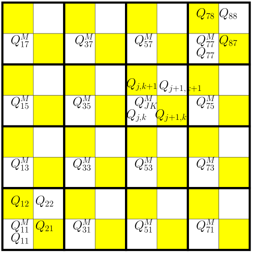
Figure 1: Macro elements: $Q_{JK}^{M}=Q_{j,k}\cup Q_{j,k+1}\cup Q_{j+1,k}\cup Q_{j+1,k+1},(J,K)=(j,k)$

We will employ capital letters to indicate odd integer indices for those macro patterns on the macro element. Owing to Theorem 2.1, the global checker–board pattern basis function ${\mathbb{C}}_{h}$ in (2.6) can be expressed explicitly as follows:

$${\mathbb{C}}_{h}=\sum_{JK}p_{JK}^{mc}.$$ (2.7)

We now try to stabilize $\boldsymbol{\mathscr{P}}_{1,0}^{nc,h}\times{\mathscr{P}}_{0}^{h}$ minimally so that the modified pairs fulfill the uniform inf-sup condition. In this section we introduce the stabilization of pressure approximation space ${\mathscr{P}}_{0}^{h}$ by eliminating one–dimensional global checker–board patterns from ${\mathscr{P}}_{0}^{h}.$ Alternatively, the stabilization of velocity approximation space $\boldsymbol{\mathscr{P}}_{1,0}^{nc,h}$, again with a globally one–dimensional modification, is given in §3.

2.3 Stabilization of ${\mathscr{P}}_{0}^{h}$

Define $\widetilde{{\mathscr{P}}_{0}^{h}}$ as the $L^{2}(\Omega)$–orthogonal complement of ${\mathscr{C}}^{h}$ in ${\mathscr{P}}_{0}^{h}$, that is,

$${\mathscr{P}}_{0}^{h}={\mathscr{C}}^{h}\oplus\widetilde{{\mathscr{P}}_{0}^{h}},\quad\operatorname{dim}\,(\widetilde{{\mathscr{P}}_{0}^{h}})=N_{Q}-2.$$ (2.8)

We are now ready to propose our Stokes element pair as follows:

$$\boldsymbol{\mathscr{P}}_{1,0}^{nc,h}\times\widetilde{{\mathscr{P}}_{0}^{h}},\quad\operatorname{dim}\,(\boldsymbol{\mathscr{P}}_{1,0}^{nc,h}\times\widetilde{{\mathscr{P}}_{0}^{h}})=2N_{v}^{i}+N_{Q}-2.$$ (2.9)

2.4 The discrete Stokes problem

Now define the discrete weak formulation of (2.2) to find a pair $(\mathbf{u}_{h},p_{h})\in\boldsymbol{\mathscr{P}}_{1,0}^{nc,h}\times\widetilde{{\mathscr{P}}_{0}^{h}}$ such that

$$a_{h}(\mathbf{u}_{h},\mathbf{v}_{h})-b_{h}(\mathbf{v}_{h},p_{h})&=({\bf f},\mathbf{v}_{h})\quad\forall\mathbf{v}_{h}\in\boldsymbol{\mathscr{P}}_{1,0}^{nc,h},\\ b_{h}(\mathbf{u}_{h},q_{h})=0\quad\qquad~{}\forall q_{h}\in\widetilde{{\mathscr{P}}_{0}^{h}},$$ (2.10)

where the discrete bilinear forms $a_{h}(\cdot,\cdot):\boldsymbol{\mathscr{P}}_{1,0}^{nc,h}\times\boldsymbol{\mathscr{P}}_{1,0}^{nc,h}\rightarrow\mathbb{R}$ and $b_{h}(\cdot,\cdot):\boldsymbol{\mathscr{P}}_{1,0}^{nc,h}\times\widetilde{{\mathscr{P}}_{0}^{h}}\rightarrow\mathbb{R}$ are defined in the standard fashion:

$$a_{h}(\mathbf{u},\mathbf{v})=\nu\sum_{j=1}^{N_{Q}}(\nabla\,\mathbf{u},\nabla\,\mathbf{v})_{Q_{j}}\quad\mbox{and}\quad b_{h}(\mathbf{v},q)=\sum_{j=1}^{N_{Q}}(\nabla\cdot\mathbf{v},q)_{Q_{j}}.$$

As usual, let $|\cdot|_{1,h}$ denote the (broken) energy semi-norm given by

$$|\mathbf{v}|_{1,h}=\sqrt{a_{h}(\mathbf{v},\mathbf{v})},$$

which is equivalent to $\|\cdot\|_{1,h}$ on $\boldsymbol{\mathscr{P}}_{1,0}^{nc,h}.$ Also, denote by $\|\cdot\|_{m,h}$ and $|\cdot|_{m,h}$ the usual mesh-dependent norm and semi-norm:

$$\|\mathbf{v}\|_{m,h}=\bigg{[}\sum_{Q\in\mathscr{T}_{h}}\|\mathbf{v}\|^{2}_{H^{m}(Q)}\bigg{]}^{1/2}\quad\mbox{and}\quad|\mathbf{v}|_{m,h}=\bigg{[}\sum_{Q\in\mathscr{T}_{h}}|\mathbf{v}|^{2}_{H^{m}(Q)}\bigg{]}^{1/2},$$

respectively. Let ${\boldsymbol{\mathscr{D}}}^{h}$ denote the divergence–free subspace of $\boldsymbol{\mathscr{P}}_{1,0}^{nc,h}$ to $\widetilde{{\mathscr{P}}_{0}^{h}}$, i.e.,

$${\boldsymbol{\mathscr{D}}}^{h}=\{\mathbf{v}_{h}\in\boldsymbol{\mathscr{P}}_{1,0}^{nc,h}~{}|~{}b_{h}(\mathbf{v}_{h},q_{h})=0,~{}\forall q_{h}\in\widetilde{{\mathscr{P}}_{0}^{h}}\}.$$ (2.11)

Then the solution $\mathbf{u}_{h}$ of (2.10) lies in ${\boldsymbol{\mathscr{D}}}^{h}$ and satisfies

$$a_{h}(\mathbf{u}_{h},\mathbf{v}_{h})=(\mathbf{f},\mathbf{v}_{h})\quad\forall\mathbf{v}_{h}\in{\boldsymbol{\mathscr{D}}}^{h}.$$ (2.12)

We state the main theorem of the paper, whose proof will be given in §4.

Theorem 2.2.

$\boldsymbol{\mathscr{P}}_{1,0}^{nc,h}\times\widetilde{{\mathscr{P}}_{0}^{h}}$ satisfies the uniform discrete inf-sup condition:

$$\sup_{{\mathbf{v}_{h}}\in\boldsymbol{\mathscr{P}}_{1,0}^{nc,h}}\frac{b_{h}({\mathbf{v}_{h}},q_{h})}{|{\mathbf{v}_{h}}|_{1,h}}\geq\beta\|q_{h}\|_{0,\Omega}\quad\forall q_{h}\in\widetilde{{\mathscr{P}}_{0}^{h}}.$$ (2.13)

3 Alternative stabilization by enriching the velocity space $\boldsymbol{\mathscr{P}}_{1,0}^{nc,h}$

In this section we consider an enrichment of $\boldsymbol{\mathscr{P}}_{1,0}^{nc,h}$ by adding a global one-dimensional bubble function space based on the quadrilateral nonconforming bubble function [5, 6, 8, 15]. We then compare two proposed nonconforming finite element space pairs $\boldsymbol{\mathscr{P}}_{1,0}^{nc,h}\times\widetilde{{\mathscr{P}}_{0}^{h}}$ and $\widetilde{\widetilde{\boldsymbol{\mathscr{P}}_{1,0}^{nc,h}}}\times{\mathscr{P}}_{0}^{h}.$ Indeed, these two spaces very closely related. The velocity solutions obtained by these two spaces are identical while the difference between the two pressures isof order $\mathscr{O}(h)$.

On a reference domain $\widehat{Q}:=[-1,1]^{2}$, the $DSSY$ nonconforming element space is defined by

$$DSSY(\widehat{Q})=\operatorname{Span}\{1,\widehat{x},\widehat{y},\theta_{k}(\widehat{x})-\theta_{k}(\widehat{y})\},$$

where

$$\theta_{k}(t)=\begin{cases}t^{2}-\frac{5}{3}t^{4},\quad&k=1,\\ t^{2}-\frac{25}{6}t^{4}+\frac{7}{2}t^{6},\quad&k=2.\end{cases}$$

Let $F_{Q}:\widehat{Q}\rightarrow Q$ be a bijective affine transformation from the reference domain onto a rectangle $Q$. Then define

$$DSSY(Q)=\left\{\widehat{v}~{}\circ~{}F_{Q}^{-1}~{}\middle|~{}\widehat{v}\in DSSY(\widehat{Q})\right\}.$$ (3.1)

The main characteristic of $DSSY(Q)$ is the edge-mean-value property:

$$\oint_{E}{\boldsymbol{\psi}}~{}ds={\boldsymbol{\psi}}(\text{midpoint of E})\quad\forall{\boldsymbol{\psi}}\in DSSY(Q),$$ (3.2)

where $\oint_{E}$ denotes $\frac{1}{|E|}\int_{E}$ [8, 15].

The vector-valued $DSSY$ nonconforming finite element space is defined by

$$&{\mathbf{DSSY}^{h}_{0}}=\{\mathbf{v}\in\mathbf{L}^{2}(\Omega)~{}|~{}\mathbf{v}_{j}:=\mathbf{v}|_{Q_{j}}\in\mathbf{DSSY}(Q_{j})~{}\forall j=1,\cdots,N_{Q};\\ \qquad\qquad\qquad\mathbf{v}\text{ is continuous at the midpoint of each interior edge }\\ \qquad\qquad\qquad~{}~{}\text{ and vanishes at the midpoint of each boundary edge in }{\mathscr{T}}_{h}\}.$$ (3.3)

For each macro element $Q_{JK}^{M},$ define ${\boldsymbol{\psi}}_{Q_{JK}^{M}}\in\mathbf{DSSY}^{h}_{0}$ such that $\operatorname{supp}({\boldsymbol{\psi}}_{Q_{JK}^{M}})\subset\overline{Q}_{JK}^{M},$ and its integral averages over the edges in ${\mathscr{T}}_{h}$ vanish except on the two edges $\partial Q_{j,\ell}\cap\partial Q_{j+1,\ell}$, $\ell=k,k+1:$

$$\oint_{\partial Q_{j,k}\cap\partial Q_{j+1,k}}{\boldsymbol{\psi}}_{Q_{JK}^{M}}~{}ds={\boldsymbol{\nu}},\qquad\oint_{\partial Q_{j,k+1}\cap\partial Q_{j+1,k+1}}{\boldsymbol{\psi}}_{Q_{JK}^{M}}~{}ds=-{\boldsymbol{\nu}}.$$

where ${\boldsymbol{\nu}}$ denotes the unit outward normal vector of $Q_{j,\ell}$ on the edge $\partial Q_{j,\ell}\cap\partial Q_{j+1,\ell}$, $\ell=k,k+1$. Define a basis function for the global bubble function, as shown in Figure 2, and a space of global bubble functions as follows:

$${\boldsymbol{\mathscr{B}}}^{h}=\operatorname{Span}\left\{{\mathbb{B}}_{h}\right\},\quad{\mathbb{B}}_{h}=\displaystyle\sum_{Q_{JK}^{M}\in{\mathscr{T}}^{M}}{\boldsymbol{\psi}}_{Q_{JK}^{M}}.$$ (3.4)

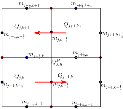
Figure 2: The basis function ${\boldsymbol{\psi}}_{Q_{JK}^{M}}\in\mathbf{DSSY}^{h}_{0}$, associated with the macro element $Q_{JK}^{M}$, takes the value ${\boldsymbol{\nu}}$ and $-{\boldsymbol{\nu}}$ at the midpoints $m_{j,k-\frac{1}{2}}$ and $m_{j,k+\frac{1}{2}},$ respectively, and value 0 at any other midpoints $m$’s shown in the figure. $Q_{J,K}^{M}=Q_{j,k}\cup Q_{j,k+1}\cup Q_{j+1,k}\cup Q_{j+1,k+1}.$

We are now ready to enrich $\boldsymbol{\mathscr{P}}_{1,0}^{nc,h}$ as follows:

$$\widetilde{\widetilde{\boldsymbol{\mathscr{P}}_{1,0}^{nc,h}}}=\boldsymbol{\mathscr{P}}_{1,0}^{nc,h}~{}\oplus~{}{\boldsymbol{\mathscr{B}}}^{h}.$$ (3.5)

Remark 3.1.

The dimension of the pair of spaces $\widetilde{\widetilde{\boldsymbol{\mathscr{P}}_{1,0}^{nc,h}}}\times{\mathscr{P}}_{0}^{h}$ is $2N_{v}^{i}+N_{Q}$.

We state the uniform inf-sup stability as in the following theorem, whose proof will be given in §4.

Theorem 3.2.

$\widetilde{\widetilde{\boldsymbol{\mathscr{P}}_{1,0}^{nc,h}}}\times{\mathscr{P}}_{0}^{h}$ satisfies the uniform discrete inf-sup condition.

3.1 Comparison between $\boldsymbol{\mathscr{P}}_{1,0}^{nc,h}\times\widetilde{{\mathscr{P}}_{0}^{h}}$ and $\widetilde{\widetilde{\boldsymbol{\mathscr{P}}_{1,0}^{nc,h}}}\times{\mathscr{P}}_{0}^{h}$

In this subsection, we will compare the two nonconforming finite element space pairs $\boldsymbol{\mathscr{P}}_{1,0}^{nc,h}\times\widetilde{{\mathscr{P}}_{0}^{h}}$ and $\widetilde{\widetilde{\boldsymbol{\mathscr{P}}_{1,0}^{nc,h}}}\times{\mathscr{P}}_{0}^{h}$. These two pairs are closely related such that $\widetilde{\widetilde{\boldsymbol{\mathscr{P}}_{1,0}^{nc,h}}}\times{\mathscr{P}}_{0}^{h}$ can be understood as a slight modification of $\boldsymbol{\mathscr{P}}_{1,0}^{nc,h}\times\widetilde{{\mathscr{P}}_{0}^{h}}$.

For $\widetilde{\widetilde{\boldsymbol{\mathscr{P}}_{1,0}^{nc,h}}}\times{\mathscr{P}}_{0}^{h}$, we have the following discrete weak formulation: Find a pair $(\mathbf{u}^{\prime}_{h},p^{\prime}_{h})\in\widetilde{\widetilde{\boldsymbol{\mathscr{P}}_{1,0}^{nc,h}}}\times{\mathscr{P}}_{0}^{h}$ such that

$$a_{h}(\mathbf{u}^{\prime}_{h},\mathbf{v}^{\prime}_{h})-b_{h}(\mathbf{v}^{\prime}_{h},p^{\prime}_{h})&=({\bf f},\mathbf{v}^{\prime}_{h})\quad\forall\mathbf{v}^{\prime}_{h}\in\widetilde{\widetilde{\boldsymbol{\mathscr{P}}_{1,0}^{nc,h}}},\\ b_{h}(\mathbf{u}^{\prime}_{h},q^{\prime}_{h})=0\quad\qquad~{}\forall q^{\prime}_{h}\in{\mathscr{P}}_{0}^{h}.$$ (3.6)

Let $\widetilde{\widetilde{\boldsymbol{\mathscr{D}}^{h}}}$ denote the divergence–free subspace of $\widetilde{\widetilde{\boldsymbol{\mathscr{P}}_{1,0}^{nc,h}}}$ to ${\mathscr{P}}_{0}^{h}$, i.e.,

$$\widetilde{\widetilde{\boldsymbol{\mathscr{D}}^{h}}}=\{\mathbf{v}^{\prime}_{h}\in\widetilde{\widetilde{\boldsymbol{\mathscr{P}}_{1,0}^{nc,h}}}~{}|~{}b_{h}(\mathbf{v}^{\prime}_{h},q^{\prime}_{h})=0,~{}\forall q^{\prime}_{h}\in{\mathscr{P}}_{0}^{h}\}.$$ (3.7)

Then the solution $\mathbf{u}^{\prime}_{h}$ of (3.6) lies in $\widetilde{\widetilde{\boldsymbol{\mathscr{D}}^{h}}}$ and satisfies

$$a_{h}(\mathbf{u}^{\prime}_{h},\mathbf{v}^{\prime}_{h})=(\mathbf{f},\mathbf{v}^{\prime}_{h})\quad\forall\mathbf{v}^{\prime}_{h}\in\widetilde{\widetilde{\boldsymbol{\mathscr{D}}^{h}}}.$$ (3.8)

The following lemma implies that the two divergence–free subspaces defined in (2.11) and (3.7) are identical, that is, our two proposed nonconforming finite element space pairs $\boldsymbol{\mathscr{P}}_{1,0}^{nc,h}\times\widetilde{{\mathscr{P}}_{0}^{h}}$ and $\widetilde{\widetilde{\boldsymbol{\mathscr{P}}_{1,0}^{nc,h}}}\times{\mathscr{P}}_{0}^{h}$ produce an identical solution for velocity.

Lemma 3.3.

The spaces ${\boldsymbol{\mathscr{D}}}^{h}$ and $\widetilde{\widetilde{\boldsymbol{\mathscr{D}}^{h}}}$ defined by (2.11) and (3.7), respectively, are equal.

Proof.

Let $\mathbf{v}_{h}\in{\boldsymbol{\mathscr{D}}}^{h}$ be given. Since $q_{h}^{\prime}\in\operatorname{Span}\{\widetilde{{\mathscr{P}}_{0}^{h}}\oplus{\mathscr{C}}^{h}\}$ and by Theorem 2.1, we get $b_{h}(\mathbf{v}_{h},q_{h}^{\prime})=0$. This implies $\mathbf{v}_{h}\in\widetilde{\widetilde{\boldsymbol{\mathscr{D}}^{h}}}$, so ${\boldsymbol{\mathscr{D}}}^{h}\subset\widetilde{\widetilde{\boldsymbol{\mathscr{D}}^{h}}}$. It remains to prove $\widetilde{\widetilde{\boldsymbol{\mathscr{D}}^{h}}}\subset{\boldsymbol{\mathscr{D}}}^{h}$. Let $\mathbf{v}_{h}^{\prime}=\mathbf{w}_{h}+\mathbf{b}_{h}\in\widetilde{\widetilde{\boldsymbol{\mathscr{D}}^{h}}}$ be given, where $\mathbf{w}_{h}\in\boldsymbol{\mathscr{P}}_{1,0}^{nc,h}$ and $\mathbf{b}_{h}\in{\boldsymbol{\mathscr{B}}}^{h}$. In particular, if we consider $q_{h}^{\prime}\in{\mathscr{C}}^{h}$, then $b_{h}(\mathbf{v}_{h}^{\prime},q_{h}^{\prime})=0$ implies $\mathbf{b}_{h}\equiv{\bf 0}$. Therefore $\mathbf{v}_{h}^{\prime}\in\boldsymbol{\mathscr{P}}_{1,0}^{nc,h}$ and $b_{h}(\mathbf{v}_{h}^{\prime},q_{h})=0$ for any $q_{h}\in\widetilde{{\mathscr{P}}_{0}^{h}}$ since $\widetilde{{\mathscr{P}}_{0}^{h}}\subset{\mathscr{P}}_{0}^{h}$. Hence $\mathbf{v}_{h}^{\prime}\in{\boldsymbol{\mathscr{D}}}^{h},$ which shows $\widetilde{\widetilde{\boldsymbol{\mathscr{D}}^{h}}}\subset{\boldsymbol{\mathscr{D}}}^{h}$. This completes the proof. ∎

Owing to Lemma 3.3, $\mathbf{u}_{h}\equiv\mathbf{u}_{h}^{\prime},$ where $\mathbf{u}_{h}$ and $\mathbf{u}_{h}^{\prime}$ are the solutions of (2.10) and (3.6), respectively. Moreover, the difference between the two pressure solutions obtained by (2.10) and (3.6) fulfills

$$b_{h}(\mathbf{v}_{h},p_{h}^{\prime}-p_{h})=0,\qquad\forall\mathbf{v}_{h}\in\boldsymbol{\mathscr{P}}_{1,0}^{nc,h}.$$

By Theorem 2.1, $p^{\prime}_{h}-p_{h}\in{\mathscr{C}}^{h}$, that is, $p^{\prime}_{h}$ can be represented by

$$p^{\prime}_{h}=p_{h}+\alpha{\mathbb{C}}_{h},\qquad\alpha\in\mathbb{R}.$$

Taking $\mathbf{v}_{h}^{\prime}={\mathbb{B}}_{h}\in{\boldsymbol{\mathscr{B}}}^{h}$ in (3.6), we obtain

$$\alpha b_{h}({\mathbb{B}}_{h},{\mathbb{C}}_{h}) = a_{h}(\mathbf{u}_{h},{\mathbb{B}}_{h})-({\bf f},{\mathbb{B}}_{h})-b_{h}({\mathbb{B}}_{h},p_{h}),$$ (3.9)

$$= \nu\displaystyle\sum_{j=1}^{N_{Q}}(\nabla\,\mathbf{u}_{h},\nabla\,{\mathbb{B}}_{h})_{Q_{j}}-({\bf f},{\mathbb{B}}_{h})-b_{h}({\mathbb{B}}_{h},p_{h}),$$

$$= \nu\displaystyle\sum_{j=1}^{N_{Q}}(-\Delta\mathbf{u}_{h},{\mathbb{B}}_{h})_{Q_{j}}+\nu\left<\frac{\partial\mathbf{u}_{h}}{\partial\mathbf{n}},{\mathbb{B}}_{h}\right>_{\partial Q_{j}}-({\bf f},{\mathbb{B}}_{h})-b_{h}({\mathbb{B}}_{h},p_{h}).$$

Since the solution $\mathbf{u}_{h}$ is a piecewise linear polynomial, that is, $\mathbf{u}_{h}\in\boldsymbol{\mathscr{P}}_{1,0}^{nc,h}$, the first term in (3.9) is equal to zero. And we easily check that the second and last terms in (3.9) turn out to vanish by the characteristics of the space ${\boldsymbol{\mathscr{B}}}^{h}$. A simple calculus using the Divergence Theorem yields

$$b_{h}({\mathbb{B}}_{h},{\mathbb{C}}_{h})=\frac{1}{h}.$$ (3.10)

Invoking (3.10), one obtains

$$\alpha=-\frac{({\bf f},{\mathbb{B}}_{h})}{b_{h}({\mathbb{B}}_{h},{\mathbb{C}}_{h})}=-h({\bf f},{\mathbb{B}}_{h}).$$ (3.11)

Hence, $p^{\prime}_{h}-p_{h}=-h(f,{\mathbb{B}}_{h}){\mathbb{C}}_{h}.$

We summarize the above result as follows:

Theorem 3.4.

Let $(\mathbf{u}_{h},p_{h})\in\boldsymbol{\mathscr{P}}_{1,0}^{nc,h}\times\widetilde{{\mathscr{P}}_{0}^{h}}$ and $(\mathbf{u}^{\prime}_{h},p^{\prime}_{h})\in\widetilde{\widetilde{\boldsymbol{\mathscr{P}}_{1,0}^{nc,h}}}\times{\mathscr{P}}_{0}^{h}$ are the solutions of (2.10) and (3.6), respectively. Then

$$\mathbf{u}_{h}=\mathbf{u}^{\prime}_{h}\quad\text{and}\quad p_{h}-p^{\prime}_{h}=-h(f,{\mathbb{B}}_{h}){\mathbb{C}}_{h}.$$ (3.12)

3.2 Interpolation operator and conference results

We recall from [21] that the global interpolation operator ${\boldsymbol{\Pi}}_{h}:\mathbf{H}^{2}(\Omega)\rightarrow\boldsymbol{\mathscr{P}}_{1}^{nc,h}$ is defined through the local interpolation operator ${\boldsymbol{\Pi}}_{Q}:\mathbf{H}^{2}(Q)\rightarrow\boldsymbol{\mathscr{P}}_{1}^{nc,h}(Q)$ such that

$${\boldsymbol{\Pi}}_{h}|_{Q}={\boldsymbol{\Pi}}_{Q}\quad\forall Q\in{\mathscr{T}}_{h}.$$

Here, ${\boldsymbol{\Pi}}_{Q}$ is explicitly defined by

$${{\boldsymbol{\Pi}}}_{Q}\mathbf{w}(M_{k})=\frac{\mathbf{w}(V_{k-1})+\mathbf{w}(V_{k})}{2}\qquad\forall\mathbf{w}\in\mathbf{H}^{2}(\Omega),$$ (3.13)

where $V_{k-1}$ and $V_{k}$ are the two vertices of the edge $E_{k}$ with midpoint $M_{k}$ of $Q$.

Define an interpolation operator $S_{h}:H^{1}(\Omega)\cap L^{2}_{0}(\Omega)\rightarrow\widetilde{{\mathscr{P}}_{0}^{h}}$ by

$$(S_{h}q,z) = (q,z)\qquad\forall z\in\widetilde{{\mathscr{P}}_{0}^{h}}.$$

Since ${\boldsymbol{\Pi}}_{h}$ and $S_{h}$ reproduce linear and constant functions on each element $Q_{j}\in{\mathscr{T}}_{h}$ and macro element $Q_{JK}^{M}$, respectively, the standard polynomial approximation results imply that

$$&\|\mathbf{v}-{\boldsymbol{\Pi}}_{h}\mathbf{v}\|_{0}+h|\mathbf{v}-{\boldsymbol{\Pi}}_{h}\mathbf{v}|_{1,h}+h^{2}|\mathbf{v}-{\boldsymbol{\Pi}}_{h}\mathbf{v}|_{2,h}\\ \qquad\qquad+h^{1/2}|\mathbf{v}-{\boldsymbol{\Pi}}_{h}\mathbf{v}|_{0,\partial\Omega}\leq Ch^{2}\|\mathbf{v}\|_{2}\quad\forall\mathbf{v}\in\mathbf{H}^{2}(\Omega),\\ \|q-S_{h}q\|_{0,\Omega}\leq Ch\|q\|_{1}\quad\forall q\in H^{1}(\Omega)\cap L^{2}_{0}(\Omega).$$ (3.14)

Owing to (3.14), a standard application of Theorems 2.2 and  3.2, and the second Strang lemma yields the following optimal error estimate:

Theorem 3.5.

Assume that (2.1) is $H^{2}(\Omega)$–regular. Let $(\mathbf{u},p)$ and $(\mathbf{u}_{h},p_{h})$ be the solutions of (2.2) and (2.10) (or (3.6)) respectively. Then the following optimal-order error estimate holds:

$$\|\mathbf{u}-\mathbf{u}_{h}\|_{0}+h\left[|\mathbf{u}-\mathbf{u}_{h}|_{1,h}+\|p-p_{h}\|_{0}\right]\leq Ch^{2}(|\mathbf{u}|_{2}+\|p\|_{1}).$$

Remark 3.6.

In the above theorem, after the result for $\boldsymbol{\mathscr{P}}_{1,0}^{nc,h}\times\widetilde{{\mathscr{P}}_{0}^{h}}$ is shown, the corresponding result for $\widetilde{\widetilde{\boldsymbol{\mathscr{P}}_{1,0}^{nc,h}}}\times{\mathscr{P}}_{0}^{h}$ to Theorem 3.5 can be obtained a combination of Theorems 3.4 and  3.5. The order of two spaces $\boldsymbol{\mathscr{P}}_{1,0}^{nc,h}\times\widetilde{{\mathscr{P}}_{0}^{h}}$ and $\widetilde{\widetilde{\boldsymbol{\mathscr{P}}_{1,0}^{nc,h}}}\times{\mathscr{P}}_{0}^{h}$ can be of course exchanged.

4 Proofs of Theorems 2.2 and  3.2

In this section we will show that $\boldsymbol{\mathscr{P}}_{1,0}^{nc,h}\times\widetilde{{\mathscr{P}}_{0}^{h}}$ and $\widetilde{\widetilde{\boldsymbol{\mathscr{P}}_{1,0}^{nc,h}}}\times{\mathscr{P}}_{0}^{h}$ satisfy the uniform discrete inf-sup condition. For this, some useful results [10, 23] will be used; in particular, Lemma 4.1, a result of Qin [23], will be utilized.

Our proof starts with setting

$${\mathscr{P}}_{c}^{h}=\left\{q_{h}\in{\mathscr{P}}_{0}^{h}~{}\middle|~{}q_{h}=\sum_{JK}a_{JK}p_{JK}^{mc},~{}\sum_{JK}a_{JK}=0\right\},\quad\operatorname{dim}\,({\mathscr{P}}_{c}^{h})=\frac{1}{4}N_{Q}-1.$$

Then denote by $W^{h}$ the $L^{2}(\Omega)$–orthogonal complement of ${\mathscr{P}}_{c}^{h}$ in ${\mathscr{P}}_{0}^{h}$ such that

$$\widetilde{{\mathscr{P}}_{0}^{h}}=W^{h}\oplus{\mathscr{P}}_{c}^{h},\quad\operatorname{dim}\,(\widetilde{{\mathscr{P}}_{0}^{h}})=N_{Q}-2\quad\text{and }\,\operatorname{dim}\,(W^{h})=\frac{3}{4}N_{Q}-1.$$ (4.1)

Let $\mathbf{Z}^{h}$ denote the discrete divergence–free subspace of $\boldsymbol{\mathscr{P}}_{1,0}^{nc,h}$ to ${\mathscr{P}}_{c}^{h}$, that is,

$$\mathbf{Z}^{h}=\left\{\mathbf{v}_{h}\in\boldsymbol{\mathscr{P}}_{1,0}^{nc,h}~{}\middle|~{}b_{h}(\mathbf{v}_{h},q_{h})=0~{}\forall q_{h}\in{\mathscr{P}}_{c}^{h}\right\}.$$

Considering the conforming bilinear element

$$\boldsymbol{\mathscr{Q}}_{1,0}^{c,h}=\left\{\mathbf{v}_{bh}\in\mathbf{H}_{0}^{1}(\Omega)~{}\middle|~{}\text{each component of }\mathbf{v}_{bh}|_{Q}\mbox{ is bilinear }~{}\forall Q\in{\mathscr{T}}_{h}\right\},$$ (4.2)

and $\mathbf{Z}_{b}^{h}$ denote the discrete divergence–free subspace of $\boldsymbol{\mathscr{Q}}_{1,0}^{c,h}$ to ${\mathscr{P}}_{c}^{h}$, that is,

$$\mathbf{Z}_{b}^{h}=\left\{\mathbf{v}_{bh}\in\boldsymbol{\mathscr{Q}}_{1,0}^{c,h}~{}\middle|~{}b_{h}(\mathbf{v}_{bh},q_{h})=0~{}\forall q_{h}\in{\mathscr{P}}_{c}^{h}\right\}.$$

Denote by $\mathscr{E}_{2h}$ and $\mathscr{E}_{2h}^{i}$ the sets of all edges and interior edges, respectively, in ${\mathscr{T}}^{M}$. Set $\boldsymbol{\mathscr{P}}_{1,0}^{me,2h}$ to be the subspace of $\boldsymbol{\mathscr{P}}_{1,0}^{nc,h}$ defined by

$$\boldsymbol{\mathscr{P}}_{1,0}^{me,2h}=\left\{\mathbf{v}_{h}\in\boldsymbol{\mathscr{P}}_{1,0}^{nc,h}~{}\middle|~{}\mathbf{v}_{h}=\displaystyle\sum_{\Gamma^{M}\in{\mathscr{E}}_{2h}}\begin{pmatrix}a_{\Gamma^{M}}\\ b_{\Gamma^{M}}\end{pmatrix}\psi_{\Gamma^{M}},\quad\begin{pmatrix}a_{\Gamma^{M}}\\ b_{\Gamma^{M}}\end{pmatrix}\in\mathbb{R}^{2}\right\},$$ (4.3)

where $\psi_{\Gamma^{M}}\in{\mathscr{P}}_{1,0}^{nc,h}$ is the basis function associated with the midpoint of the macro edge $\Gamma^{M}\in{\mathscr{E}}^{i}_{2h}$ as described in detail in the caption of Figure 3. Notice that $\operatorname{dim}\,(\boldsymbol{\mathscr{P}}_{1,0}^{me,2h})=N_{v}^{i}-1.$

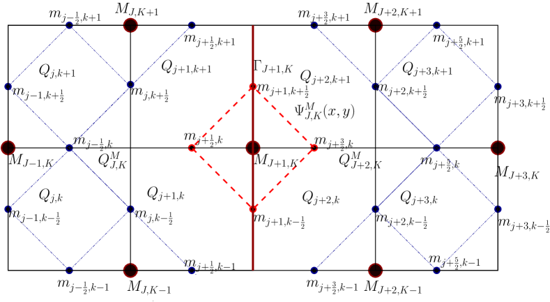
Figure 3: The basis function $\psi_{\Gamma^{M}}\in\boldsymbol{\mathscr{P}}_{1,0}^{nc,h}$, associated with the macro edge $\Gamma^{M}=\Gamma_{J+1,K}^{M}$, takes value 1 along the four line segments joining the midpoints $m_{j+\frac{3}{2},k},m_{j+1,k+\frac{1}{2}},m_{j+\frac{1}{2},k},$ and $m_{j+1,k-\frac{1}{2}}$, and value 0 at any other midpoints $m$’s shown in the figure. $M_{J+1,K}$ denotes the midpoint of the macro edge $\Gamma_{J+1,K}^{M}$, the common edge of the two macro elements $Q_{J,K}^{M}$ and $Q_{J+2,K}^{M}$, with $Q_{J,K}^{M}=Q_{j,k}\cup Q_{j,k+1}\cup Q_{j+1,k}\cup Q_{j+1,k+1}$ and $Q_{J+2,K}^{M}=Q_{j+2,k}\cup Q_{j+2,k+1}\cup Q_{j+3,k}\cup Q_{j+3,k+1}.$

Next, we quote the Subspace Theorem of Qin as in the following lemma:

Lemma 4.1 ([23]).

Given $\mathbf{V}^{h}\times P^{h}$, let $\mathbf{V}_{1}$ and $\mathbf{V}_{2}$ be two subspaces of $\mathbf{V}^{h}$ and $P_{1}$ and $P_{2}$ be two subspaces of $P^{h}$. Let the following four conditions hold:

1. $P^{h}$ $=P_{1}+P_{2};$

2. there exist $\beta_{j}>0,j=1,2$, independent of $h$, such that

   $$\sup_{{\mathbf{v}_{j}}\in\mathbf{V}_{j}}\frac{b_{h}({\mathbf{v}_{j}},q_{j})}{|{\mathbf{v}_{j}}|_{1,h}} \geq \beta_{j}\|q_{j}\|_{0,\Omega},\quad\forall q_{j}\in P_{j},$$

3. there exist $\alpha_{j}\geq 0,j=1,2,$ such that

   $$|b_{h}(\mathbf{v}_{j},q_{k})| \leq \alpha_{j}|\mathbf{v}_{j}|_{1,h}\|q_{k}\|_{0,\Omega},\quad\forall\mathbf{v}_{j}\in\mathbf{V}_{j}\mbox{ and }\forall q_{k}\in P_{k},\,j,k=1,2;j\neq k,$$

   with

   $$\alpha_{1}\alpha_{2}\leq\beta_{1}\beta_{2}.$$

Then, $\mathbf{V}^{h}\times P^{h}$ satisfies the inf-sup condition with the inf-sup constant depending only on $\alpha_{1},\alpha_{2},\beta_{1},\beta_{2}$.

4.1 Proof of Theorem 2.2

The following lemma is an immediate consequence of the Divergence Theorem, which will be useful to prove Lemma 4.3:

Lemma 4.2.

Let $Q\subset\mathbb{R}^{2}$ be a rectangular domain. Suppose that $\mathbf{w}$ is a two–variable function whose components are bilinear polynomials on $Q$. Then the following holds:

$$\int_{Q}\nabla\cdot\mathbf{w}~{}dA=\int_{Q}\nabla\cdot{\boldsymbol{\Pi}}_{Q}\mathbf{w}~{}dA.$$

Lemma 4.3.

$\mathbf{Z}^{h}\times W^{h}$ satisfies the uniform discrete inf-sup condition:

$$\sup_{{\mathbf{v}_{h}}\in\mathbf{Z}^{h}}\frac{b_{h}({\mathbf{v}_{h}},q_{h})}{|{\mathbf{v}_{h}}|_{1,h}}\geq\beta\|q_{h}\|_{0,\Omega}\quad\forall q_{h}\in W^{h}.$$ (4.4)

Proof.

We begin with invoking [4] that $\mathbf{Z}_{b}^{h}\times W^{h}$ satisfies the uniform inf-sup condition, that is, there exists a positive constant $\beta$ independent of $h$ such that

$$\sup_{{\mathbf{v}_{bh}}\in\mathbf{Z}_{b}^{h}}\frac{b_{h}({\mathbf{v}_{bh}},q_{h})}{|{\mathbf{v}_{bh}}|_{1,h}}\geq\beta\|q_{h}\|_{0,\Omega}\quad\forall q_{h}\in W^{h}.$$ (4.5)

Let $q_{h}\in W^{h},q_{h}\neq 0$ be arbitrary. Then, (4.5) is equivalent (cf. [10], p. 118) to the existence of $\mathbf{v}_{bh}\in\mathbf{Z}_{b}^{h}$ such that

$$b_{h}(\mathbf{v}_{bh},q_{h})=\|q_{h}\|_{0,\Omega}^{2},\\ |\mathbf{v}_{bh}|_{1,\Omega}\leq\frac{1}{\beta}\|q_{h}\|_{0,\Omega}.$$ (4.6)

Now Lemma 4.2 implies that ${\boldsymbol{\Pi}}_{h}\mathbf{v}_{bh}\in\mathbf{Z}^{h}$ and

$$b_{h}({\boldsymbol{\Pi}}_{h}\mathbf{v}_{bh},q_{h})=b_{h}(\mathbf{v}_{bh},q_{h})=\|q_{h}\|_{0,\Omega}^{2}.$$ (4.7)

By Young’s inequality, the definition of interpolation operator ${\boldsymbol{\Pi}}_{h}$ and (4.6), one sees that

$$|{\boldsymbol{\Pi}}_{h}\mathbf{v}_{bh}|_{1,h}\leq C|\mathbf{v}_{bh}|_{1,\Omega}\leq\frac{C}{\beta}\|q_{h}\|_{0,\Omega},$$ (4.8)

where the constant $C$ is independent of mesh size $h$. Notice that the element of $\mathbf{v}_{h}={\boldsymbol{\Pi}}_{h}\mathbf{v}_{bh}\in\mathbf{Z}^{h}$ satisfying (4.7) and (4.8) plays a role of an equivalent statement to (4.4). Hence the lemma is complete. ∎

Lemma 4.4.

$\boldsymbol{\mathscr{P}}_{1,0}^{me,2h}\times{\mathscr{P}}_{c}^{h}$ satisfies the uniform discrete inf-sup condition:

$$\sup_{{\mathbf{v}}_{h}\in\boldsymbol{\mathscr{P}}_{1,0}^{me,2h}}\frac{b_{h}({\mathbf{v}}_{h},q_{h})}{|{\mathbf{v}}_{h}|_{1,h}}\geq\beta\|q_{h}\|_{0,\Omega}\quad\forall q_{h}\in{\mathscr{P}}_{c}^{h}.$$ (4.9)

Proof.

Set

$${\mathscr{P}}_{0}^{2h}=\{q\in L^{2}_{0}(\Omega)\,\mid~{}q|_{Q^{M}}\in P_{0}(Q^{M})~{}\forall Q^{M}\in{\mathscr{T}}^{M}\},\quad\operatorname{dim}\,({\mathscr{P}}_{0}^{2h})=N_{Q}/4-1.$$

Due to Lemma 3.1 in [22], $\boldsymbol{\mathscr{P}}_{1,0}^{me,2h}\times{\mathscr{P}}_{0}^{2h}$ satisfies the uniform inf-sup condition, that is, there exists a positive constant $\beta$ independent of $h$ such that

$$\sup_{\overline{\mathbf{v}}_{h}\in\boldsymbol{\mathscr{P}}_{1,0}^{me,2h}}\frac{b_{h}(\overline{\mathbf{v}}_{h},\overline{q}_{h})}{|\overline{\mathbf{v}}_{h}|_{1,h}}\geq\beta\|\overline{q}_{h}\|_{0,\Omega}\quad\forall\overline{q}_{h}\in{\mathscr{P}}_{0}^{2h}.$$ (4.10)

Let $q_{h}=\displaystyle\sum_{JK}\alpha_{JK}p_{JK}^{mc}\in{\mathscr{P}}_{c}^{h}$ be arbitrary. Consider $\overline{q}_{h}=\displaystyle\sum_{JK}\alpha_{JK}p_{JK}\in{\mathscr{P}}_{0}^{2h},$ where $p_{JK}=\chi_{Q_{JK}^{M}}.$ Then there exists $\overline{\mathbf{v}}_{h}=\displaystyle\sum_{\Gamma^{M}\in{\mathscr{E}}_{2h}}\begin{pmatrix}a_{\Gamma^{M}}\\ b_{\Gamma^{M}}\end{pmatrix}\psi_{\Gamma^{M}}\in\boldsymbol{\mathscr{P}}_{1,0}^{me,2h}$ such that (4.10) holds. From this $\overline{\mathbf{v}}_{h}$, we define $\mathbf{v}_{h}\in\boldsymbol{\mathscr{P}}_{1,0}^{me,2h}$ as follows:

$$\mathbf{v}_{h}=-\displaystyle\sum_{\Gamma^{M}\in{\mathscr{E}}_{2h}}\begin{pmatrix}b_{\Gamma^{M}}\\ a_{\Gamma^{M}}\end{pmatrix}\psi_{\Gamma^{M}}.$$

Then the following three equalities are obvious:

$$\|q_{h}\|_{0,\Omega}&=\|\overline{q}_{h}\|_{0,\Omega},\\ |\mathbf{v}_{h}|_{1,h}=|\overline{\mathbf{v}}_{h}|_{1,h},\\ b_{h}(\mathbf{v}_{h},q_{h})=b_{h}(\overline{\mathbf{v}}_{h},\overline{q}_{h}).$$ (4.11)

From (4.10) and (4.11), the inf-sup condition (4.9) for $\boldsymbol{\mathscr{P}}_{1,0}^{me,2h}\times{\mathscr{P}}_{c}^{h}$ follows. This proves our assertion. ∎

Utilizing Lemma 4.1, we are ready to prove Theorem 2.2.

Proof of Theorem 2.2..

We will check the conditions of Lemma 4.1. Let $\mathbf{V}_{1}=\mathbf{Z}^{h},~{}\mathbf{V}_{2}=\boldsymbol{\mathscr{P}}_{1,0}^{me,2h}$ and $P_{1}=W^{h},~{}P_{2}={\mathscr{P}}_{c}^{h}$. Obviously, $\mathbf{V}_{j}$ and $P_{j},~{}j=1,2$ are subspaces of $\boldsymbol{\mathscr{P}}_{1,0}^{nc,h}$ and $\widetilde{{\mathscr{P}}_{0}^{h}}$, respectively, so that Condition (1) holds. Moreover, Lemmas 4.3 and  4.4 imply that Condition (2) holds. Since $b_{h}(\mathbf{v}_{1},q_{2})=0$ holds for any $\mathbf{v}_{1}\in\mathbf{V}_{1}$ and any $q_{2}\in P_{2}$, one has $\alpha_{1}=0$. Consequently, Condition (3) holds. Hence by Lemma 4.1, $\boldsymbol{\mathscr{P}}_{1,0}^{nc,h}\times\widetilde{{\mathscr{P}}_{0}^{h}}$ satisfies the inf-sup condition (2.13). ∎

4.2 Proof of Theorem 3.2

In order to prove Theorem 3.2, the following lemma is needed.

Lemma 4.5.

${\boldsymbol{\mathscr{B}}}^{h}\times{\mathscr{C}}^{h}$ satisfies the inf-sup condition, that is, there exists a positive constant $\beta$ independent of $h$ such that

$$\sup_{{\mathbf{v}}_{h}\in{\boldsymbol{\mathscr{B}}}^{h}}\frac{b_{h}({\mathbf{v}}_{h},q_{h})}{|{\mathbf{v}}_{h}|_{1,h}}\geq\beta\|q_{h}\|_{0,\Omega}\quad\forall q_{h}\in{\mathscr{C}}^{h}.$$ (4.12)

Proof.

Let $q_{h}\in{\mathscr{C}}^{h}$ be given by $q_{h}=\alpha{\mathbb{C}}_{h}$ with a constant $\alpha\in\mathbb{R},$ and set $\mathbf{v}_{h}={\mathbb{B}}_{h}\in{\boldsymbol{\mathscr{B}}}^{h}.$ Recall (3.10) so that

$$b_{h}(\mathbf{v}_{h},q_{h})=\frac{\alpha}{h}.$$ (4.13)

Also, it is trivial to see

$$\|q_{h}\|_{0,\Omega}=|\alpha|.$$ (4.14)

It remains to compute $|\mathbf{v}_{h}|_{1,h}$. For this, we notice that $|\mathbf{v}_{h}|_{1,Q}$ does not depend on the mesh size $h$ of $Q$, since it is a two dimensional region. Indeed, there exists a constant $C_{1}$ independent of $h$ such that $|\mathbf{v}_{h}|_{1,h}^{2}=\displaystyle\sum_{Q\in{\mathscr{T}}_{h}}\int_{Q}|\nabla\,\mathbf{v}_{h}|^{2}~{}d{\mathbf{x}}=\frac{C_{1}}{h^{2}}.$ Hence, we get

$$|\mathbf{v}_{h}|_{1,h}=\frac{C}{h},\qquad\text{where }C=\sqrt{C_{1}}.$$ (4.15)

Now, the combination of (4.13), (4.14) and (4.15) leads to (4.12) with the inf-sup constant $\beta=1/C$. This completes the proof. ∎

Theorem 3.2 is now ready to be shown, by using Lemmas 4.1 and  4.5.

Proof of Theorem 3.2..

Let $\mathbf{V}_{1}=\boldsymbol{\mathscr{P}}_{1,0}^{nc,h},~{}\mathbf{V}_{2}={\boldsymbol{\mathscr{B}}}^{h}$ and $P_{1}=\widetilde{{\mathscr{P}}_{0}^{h}},~{}P_{2}={\mathscr{C}}^{h}$. Since ${\mathscr{P}}_{0}^{h}=\widetilde{{\mathscr{P}}_{0}^{h}}\oplus{\mathscr{C}}^{h}$, Condition $(1)$ in Lemma 4.1 holds. Moreover, Theorem 2.2 and Lemma 4.5 imply Condition $(2)$ holds. Finally, $b_{h}(\mathbf{v}_{1},q_{2})=0$ holds for any $\mathbf{v}_{1}\in\mathbf{V}_{1}$ and $q_{2}\in P_{2}$ by Theorem 2.1, which implies that $\alpha_{1}=0.$ Consequently, Condition $(3)$ holds. Hence, $\widetilde{\widetilde{\boldsymbol{\mathscr{P}}_{1,0}^{nc,h}}}\times{\mathscr{P}}_{0}^{h}$ satisfies the inf-sup condition. Note that the constant in each step is independent of $h$. ∎

5 Numerical results

Now we illustrate a numerical example for the stationary Stokes problem on uniform meshes on the domain $\Omega=(0,1)^{2}.$ Throughout this numerical study, we fix $\nu=1$.

First we calculate the discrete inf-sup constants of various finite element pairs including our suggestions.

In contrast to the $\mathscr{O}(h)$–dependent inf-sup constant of conforming bilinear and piecewise constant finite element pair [3, 4], our two proposed nonconforming finite elements satisfy the uniform inf-sup condition at least on square meshes. To confirm theoretical analysis, we give the numerical results of the discrete inf-sup constants [19] in Table 1.

$h$	$\beta_{1}$	Order	$\beta_{2}$	Order	$\beta_{3}$	Order
${1}/{4}$	4.9642E-01	-	4.9560E-01	-	5.0000E-01	-
${1}/{8}$	2.8605E-01	0.78	4.6791E-01	0.08	4.6746E-01	0.09
${1}/{16}$	1.5029E-01	0.93	4.4415E-01	0.07	4.5296E-01	0.04
${1}/{32}$	7.6544E-02	0.97	4.2863E-01	0.05	4.4526E-01	0.02
${1}/{64}$	3.8562E-02	0.99	4.1864E-01	0.03	4.4051E-01	0.02

Table 1: Estimation of the inf-sup constants $\beta_{j},j=1,2,3,$ for the three finite element pairs $\boldsymbol{\mathscr{Q}}_{1,0}^{c,h}\times\widetilde{{\mathscr{P}}_{0}^{h}}$, $\boldsymbol{\mathscr{P}}_{1,0}^{nc,h}\times\widetilde{{\mathscr{P}}_{0}^{h}}$, and $\widetilde{\widetilde{\boldsymbol{\mathscr{P}}_{1,0}^{nc,h}}}\times{\mathscr{P}}_{0}^{h}.$

We will borrow the two numerical examples from [22]. The source term ${\bf f}$ is generated by the choice of the exact solution.

$$\mathbf{u}(x,y)=(s(x)s^{\prime}(y),-s(y)s^{\prime}(x)),\qquad p(x,y)=\sin(2\pi x)f(y),$$ (5.1)

where $s(t)=\sin(2\pi t)(t^{2}-t)$ and $s^{\prime}(t)$ denotes its derivative. The velocity $\mathbf{u}$ vanishes on $\partial\Omega$ and the pressure $p$ has mean value zero regardless of $f$.

Several interesting numerical results for the pair $\boldsymbol{\mathscr{P}}_{1,0}^{nc,h}\times\widetilde{{\mathscr{P}}_{0}^{h}}$ are presented, while the corresponding numerical results for the pair $\widetilde{\widetilde{\boldsymbol{\mathscr{P}}_{1,0}^{nc,h}}}\times{\mathscr{P}}_{0}^{h}$ are omitted here, since they behave quite similarly to those case for the pair $\boldsymbol{\mathscr{P}}_{1,0}^{nc,h}\times\widetilde{{\mathscr{P}}_{0}^{h}}$. Numerical results with $f(y)=\frac{1}{3-\tan^{2}y}$ are shown in Table 2. We observe optimal order of convergence in both velocity and pressure variables. Also numerical experiments are carried out and presented in (5.1) for $f(y)=\frac{1}{25-10\tan^{2}y}+\frac{3}{10}$ which has a huge slope near the boundary on $y=1$. Since the pressure changes rapidly on the boundary $y=1$, convergence rates show a poor approximation in coarse meshes in Table 3. However, as the meshes get finer, optimal order convergence is observed as expected from the inf-sup condition.

h	$|\mathbf{u}-\mathbf{u}_{h}|_{1,h}$	Order	$\|\mathbf{u}-\mathbf{u}_{h}\|_{0}$	Order	$\|p-p_{h}\|_{0}$	Order
1/4	1.5087E-0	-	2.1583E-1	-	2.2190E-1	-
1/8	8.1269E-1	0.8926	5.5033E-2	1.9715	1.4098E-1	0.6544
1/16	4.1360E-1	0.9745	1.3930E-2	1.9821	6.4738E-2	1.1229
1/32	2.0767E-1	0.9939	3.4936E-3	1.9954	3.2509E-2	0.9938
1/64	1.0394E-1	0.9985	8.7411E-4	1.9988	1.6411E-2	0.9862
1/128	5.1985E-2	0.9996	2.1857E-4	1.9997	8.2359E-3	0.9947
1/256	2.5994E-2	0.9999	5.4646E-5	1.9999	4.1222E-3	0.9985
1/512	1.2997E-2	1.0000	1.3661E-5	2.0000	2.0616E-3	0.9996
1/1024	6.4987E-3	1.0000	3.4154E-6	2.0000	1.0309E-3	0.9999

Table 2: Numerical results for uniform meshes with $f(y)=\frac{1}{3-\tan^{2}y}$

h	$|\mathbf{u}-\mathbf{u}_{h}|_{1,h}$	Order	$\|\mathbf{u}-\mathbf{u}_{h}\|_{0}$	Order	$\|p-p_{h}\|_{0}$	Order
1/4	1.5086E-0	-	2.1578E-1	-	1.7459E-1	-
1/8	8.1268E-1	0.8925	5.5016E-2	1.9716	1.1835E-1	0.5609
1/16	4.1360E-1	0.9744	1.3926E-2	1.9820	5.7158E-2	1.0501
1/32	2.0767E-1	0.9939	3.4938E-3	1.9950	3.6347E-2	0.6531
1/64	1.0394E-1	0.9985	8.7450E-4	1.9983	2.3178E-2	0.6491
1/128	5.1985E-2	0.9996	2.1872E-4	1.9993	1.3569E-2	0.7725
1/256	2.5994E-2	0.9999	5.4690E-5	1.9998	7.3091E-3	0.8925
1/512	1.2997E-2	1.0000	1.3673E-5	1.9999	3.7516E-3	0.9622
1/1024	6.4987E-3	1.0000	3.4183E-6	2.0000	1.8899E-3	0.9892

Table 3: Numerical results for uniform meshes with $f(y)=\frac{1}{25-10\tan^{2}y}+\frac{3}{10}$

The following numerical results highlight the reliability of our proposed finite element space compared to the case of using the conforming bilinear element for the approximation of the velocity field. Recall that the pair of conforming finite element space combined with the piecewise constant element space $\boldsymbol{\mathscr{Q}}_{1,0}^{c,h}\times\widetilde{{\mathscr{P}}_{0}^{h}}$ is unstable unless $\mathbf{f}$ is smooth enough as quoted in the following Corollary:

Corollary 5.1 (Boland and Nicolaides, Cor. 6.1 in [4]).

For $\beta\in(0,1),$ there exists $\mathbf{f}\in\mathbf{L}^{2}(\Omega)$ such that the pressure approximation to (2.2) by using $\boldsymbol{\mathscr{Q}}_{1,0}^{c,h}\times\widetilde{{\mathscr{P}}_{0}^{h}}$ fulfills

$$\|p-p_{h}\|_{0}\geq Ch^{\beta}\|\mathbf{f}\|_{0}\qquad\text{for }h\leq h_{\beta}$$ (5.2)

for some $h_{\beta}>0,$ independent of $h.$

With $\beta=0.3$ fixed, some comparative numerical results for conforming and nonconforming pairs using $\boldsymbol{\mathscr{Q}}_{1,0}^{c,h}\times\widetilde{{\mathscr{P}}_{0}^{h}}$ and $\boldsymbol{\mathscr{P}}_{1,0}^{nc,h}\times\widetilde{{\mathscr{P}}_{0}^{h}}$ are shown in Tables 4 and  5, respectively. These results ensure the superiority of our nonconforming method over the conforming counterpart.

Throughout our numerical experiments, the $4\times 4$ Gauss quadrature rule is adopted for each rectangular element. The approximate data for $\bf f$ are calculated by following the proof of Theorem 6.1 in [4] at the $4\times 4$ Gauss points in each element of $512\times 512$ mesh. The reference solutions used in error calculation are obtained by using the $DSSY$ element [8] with the $512\times 512$ mesh. The graphs of components of $\mathbf{f}$ are given in Figure 4.

Remark 5.2.

It should be stressed that the degrees of freedom for both $\boldsymbol{\mathscr{Q}}_{1,0}^{c,h}\times\widetilde{{\mathscr{P}}_{0}^{h}}$ and $\boldsymbol{\mathscr{P}}_{1,0}^{nc,h}\times\widetilde{{\mathscr{P}}_{0}^{h}}$ are essentially identical, although numerical results are quite different. Further investigations need to be sought to analyze the differences between the conforming bilinear element and the $P_{1}$ nonconforming element.

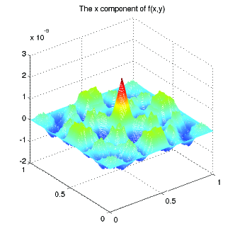
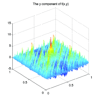
Figure 4: The graph of data $\bf f$

h	$|\mathbf{u}_{ref}-\mathbf{u}_{h}|_{1,h}$	order	$\|\mathbf{u}_{ref}-\mathbf{u}_{h}\|_{0}$	order	$\|p_{ref}-p_{h}\|_{0}$	order
1/4	2.8248E-2	-	1.8470E-3	-	7.2967E-2	-
1/8	1.6008E-2	0.8193	5.3114E-4	1.7981	5.6105E-2	0.3791
1/16	8.5909E-3	0.8980	1.4266E-4	1.8964	4.1920E-2	0.4205
1/32	4.4824E-3	0.9385	3.7531E-5	1.9265	3.1925E-2	0.3929
1/64	2.3084E-3	0.9573	9.6932E-6	1.9531	2.4932E-2	0.3567
1/128	1.1939E-3	0.9512	2.4703E-6	1.9722	1.9829E-2	0.3304
1/256	6.4542E-4	0.8874	6.2940E-7	1.9727	1.5938E-2	0.3152

Table 4: Numerical results for $\boldsymbol{\mathscr{Q}}_{1,0}^{c,h}\times\widetilde{{\mathscr{P}}_{0}^{h}}$ when $\beta=0.3$

h	$|\mathbf{u}_{ref}-\mathbf{u}_{h}|_{1,h}$	order	$\|\mathbf{u}_{ref}-\mathbf{u}_{h}\|_{0}$	order	$\|p_{ref}-p_{h}\|_{0}$	order
1/4	2.8359E-2	-	1.8561E-3	-	4.9406E-2	-
1/8	1.7966E-2	0.6585	5.0224E-4	1.8858	2.6963E-2	0.8737
1/16	1.0379E-2	0.7916	1.3390E-4	1.9072	1.4305E-2	0.9144
1/32	5.6226E-3	0.8844	3.5144E-5	1.9298	7.5726E-3	0.9177
1/64	2.9406E-3	0.9351	9.0617E-6	1.9554	3.9235E-3	0.9486
1/128	1.5002E-3	0.9710	2.3029E-6	1.9763	1.9663E-3	0.9966
1/256	7.3601E-4	1.0274	5.7096E-7	2.0120	8.9372E-4	1.1376

Table 5: Numerical results for $\boldsymbol{\mathscr{P}}_{1,0}^{nc,h}\times\widetilde{{\mathscr{P}}_{0}^{h}}$ when $\beta=0.3$

References

- [1] D. N. Arnold, F. Brezzi, and M. Fortin. A stable finite element for the Stokes equations. Calcolo, 21:337–344, 1984.
- [2] C. Bernardi and G. Raguel. Analysis of some finite elements for the Stokes problem. Math. Comp., 44:71–80, 1985.
- [3] J. M. Boland and R. A. Nicolaides. On the stability of bilinear-constant velocity-pressure finite elements. Numer. Math., 44(2):219–222, 1984.
- [4] J. M. Boland and R. A. Nicolaides. Stable and semistable low order finite elements for viscous flows. SIAM J. Numer. Anal., 22(3):474–492, 1985.
- [5] Z. Cai, J. Douglas, Jr., J. E. Santos, D. Sheen, and X. Ye. Nonconforming quadrilateral finite elements: A correction. Calcolo, 37(4):253–254, 2000.
- [6] Z. Cai, J. Douglas, Jr., and X. Ye. A stable nonconforming quadrilateral finite element method for the stationary Stokes and Navier-Stokes equations. Calcolo, 36:215–232, 1999.
- [7] M. Crouzeix and P.-A. Raviart. Conforming and nonconforming finite element methods for solving the stationary Stokes equations. R.A.I.R.O.– Math. Model. Anal. Numer., R-3:33–75, 1973.
- [8] J. Douglas, Jr., J. E. Santos, D. Sheen, and X. Ye. Nonconforming Galerkin methods based on quadrilateral elements for second order elliptic problems. ESAIM–Math. Model. Numer. Anal., 33(4):747–770, 1999.
- [9] M. Engelman, R. L. Sani, P. M. Gresho, and M. Bercovier. Consistent vs. reduced integration penalty methods for the incompressible media using several old and new elements. Int. J. Numer. Meth. Fluids, 1:347–364, 1981.
- [10] V. Girault and P.-A. Raviart. Finite Element Methods for Navier–Stokes Equations, Theory and Algorithms. Springer-Verlag, Berlin, 1986.
- [11] R. Glowinski and O. Pironneau. On a mixed finite element approximation of the Stokes problem. I. Convergence of the approximate solutions. Numer. Math., 33:397–424, 1979.
- [12] H. Han. Nonconforming elements in the mixed finite element method. J. Comp. Math., 2:223–233, 1984.
- [13] P. Hood and C. Taylor. A numerical solution for the Navier-Stokes equations using the finite element technique. Comp. Fluids, 1:73–100, 1973.
- [14] J. Hu, H.-Y. Man, and Z.-C. Shi. Constrained nonconforming rotated element for Stokes and planar elasticity. Math. Numer. Sin. (in Chinese), 27:311–324, 2005.
- [15] Y. Jeon, H. Nam, D. Sheen, and K. Shim. A class of nonparametric DSSY nonconforming quadrilateral elements. ESAIM–Math. Model. Numer. Anal., 47(06):1783–1796, 2013.
- [16] S. Kim and D. Sheen. A stable cheapest nonconforming finite element for the Stokes–Darcy–Brinkman interface problem. 2015. to appear.
- [17] R. Lim and D. Sheen. Nonconforming finite element method applied to the driven cavity problem. 2015. to appear.
- [18] H. Liu and N. Yan. Superconvergence analysis of the nonconforming quadrilateral linear-constant scheme for Stokes equations. Adv. Comput. Math., 29:375–392, 2008.
- [19] D. S. Malkus. Eigenproblems associated with the discrete LBB condition for incompressible finite elements. International Journal of Engineering Science, 19(10):1299–1310, 1981.
- [20] H. Nam, H. J. Choi, C. Park, and D. Sheen. A cheapest nonconforming rectangular finite element for the Stokes problem. Comput. Methods Appl. Mech. Engrg., 257:77–86, 2013.
- [21] C. Park and D. Sheen. -nonconforming quadrilateral finite element methods for second-order elliptic problems. SIAM J. Numer. Anal., 41(2):624–640, 2003.
- [22] C. Park, D. Sheen, and B.-C. Shin. A subspace of the DSSY nonconforming quadrilateral finite element space for the incompressible Stokes equations. J. Comput. Appl. Math., 239:220–230, 2013.
- [23] J. Qin. On the Convergence of Some Low Order Mixed Finite Elements for Incompressible Fluids. PhD thesis, Department of Mathematics, Pennsylvania State University, University Park, PA 16802. Thesis advisor, Douglas N. Arnold, 1994.
- [24] R. Rannacher and S. Turek. Simple nonconforming quadrilateral Stokes element. Numer. Methods Partial Differential Equations, 8:97–111, 1992.
- [25] R. Stenberg. Analysis of mixed finite element methods for the Stokes problem: A unified approach. Math. Comp., 42:9–23, 1984.
- [26] R. Stenberg. Some problems in connection with the finite element solution of Navier-Stokes equations. In J. Hallikas, M. L. Kanervirta, and P. Neittaanmaki, editors, Proceedings of the Conference on Numerical Simulation Models, pages 194–212, Espoo, 1987. Technical Research Center of Finland.