From reversible computation to quantum computation by Lagrange interpolation

Abstract

Classical reversible circuits, acting on $w$ bits, are represented by permutation matrices of size $2^{w}\times 2^{w}$. Those matrices form the group P($2^{w}$), isomorphic to the symmetric group S${}_{2^{w}}$. The permutation group P($n$), isomorphic to S_n, contains cycles with length $p$, ranging from 1 to $L(n)$, where $L(n)$ is the so-called Landau function. By Lagrange interpolation between the $p$ matrices of the cycle, we step from a finite cyclic group of order $p$ to a 1-dimensional Lie group, subgroup of the unitary group U($n$). As U($2^{w}$) is the group of all possible quantum circuits, acting on $w$ qubits, such interpolation is a natural way to step from classical computation to quantum computation.

1 Introduction

Too often conventional (every-day) computers and (futuristic) quantum computers are considered as two separate worlds, far from each other. Conventional computers act on classical bits, say ‘pure’ zeroes and ones, by means of Boolean logic gates, such as AND gates and OR gates [1]. The operations performed by these gates usually are described by truth tables. Quantum computers act on qubits, say complex vectors, by means of quantum gates, such as ROTATOR gates and T gates [2]. The operations performed by these gates usually are described by unitary matrices.

Because the world of classical computation and the world of quantum computation are based on such different science models, it is difficult to see the relationship (both analogies and differences) between these two computation paradigms. In order to remedy this problem, in recent years, NEGATOR gates and PHASOR gates have been developed as basic building-blocks of quantum circuits [3] [4] [5]. In the present paper, we bridge the gap between the two sciences by deriving the NEGATOR gates in an alternative way. The common tool we have chosen for describing both reversible computation and quantum computation is the matrix representation. Classical reversible circuits [1], acting on $w$ bits, are represented by permutation matrices of size $2^{w}\times 2^{w}$, whereas quantum circuits [2], acting on $w$ qubits, are represented by unitary matrices of size $2^{w}\times 2^{w}$. Invertible matrices form a group under the operation of matrix multiplication. The matrix group consisting of permutation matrices is a subgroup of the group of unitary matrices. In the present paper, we show how to enlarge the subgroup to its supergroup, in other words: how a classical computer can be upgraded to a quantum computer. It is surprising that a mathematical tool for this tour-de-force is the good-old polynomial interpolation formula of Lagrange. By Lagrange interpolation between two (or more) permutation matrices we indeed obtain an infinity of unitary matrices.

2 The Lagrange interpolation

We consider the $n\times n$ unitary matrix $q$. The only restriction is the finiteness of its order. In other words: we assume that $q^{\,p}$ equals the $n\times n$ unit matrix $u$ and that none of the matrices $q^{\,s}$ with $0<s<p$ equals $u$. Thus the set $\{q,q^{2},q^{3},...,q^{p-1},q^{p}\}$ (with $q^{p}=q^{0}=u$) constitutes a finite matrix group isomorphic to the cyclic group Z_p of order $p$.

We construct a 1-dimensional Lie group which constitutes a smooth interpolation between the $p$ matrices $q^{j}$. For this purpose, we are inspired by the interpolation formula of Lagrange: if, for the values $x=x_{j}$, a function $y(x)$ evaluates to $y_{j}$, then the polynomial

$$p(x)=\sum_{j}\ \frac{\prod_{k\neq j}(x-x_{k})}{\prod_{k\neq j}(x_{j}-x_{k})}\ y_{j}$$

automatically satisfies $p(x_{j})=y_{j}$, for all $x_{j}$. The function $p(x)$ connects the points $(x_{j},y_{j})$ in an analytic and smooth way. By analogy, we construct the matrix

$$m(\theta)=\sum_{j}\ \frac{\prod_{k\neq j}(e^{i\theta}-\omega^{k})}{\prod_{k\neq j}(\omega^{j}-\omega^{k})}\ q^{j}\ ,$$ (1)

where the constant $\omega$ is the primitive $p$ th root of unity, i.e. $e^{i2\pi/p}$. Here, indices ($j$ and $k$) run from 0 to $p-1$. The reader can easily verify that indeed we automatically have $m(j\,2\pi/p)=q^{j}$. In particular we have $m(0)=q^{0}=u$. Expression (1) constitutes a generalization of the case $p=2$, discussed in Appendix A of [5]. Indeed, for $p=2$, eqn (1) recovers the expression found in [5]:

$$m(\theta)=\frac{1+e^{i\theta}}{2}\ q^{0}+\frac{1-e^{i\theta}}{2}\ q^{1}\ .$$ (2)

Rewriting (1) as

$$m(\theta)=\sum_{j}m_{j}(\theta)\,q^{j}\ ,$$ (3)

the coefficients $m_{j}(\theta)$ (known as the Lagrange basis polynomials or Lagrange fundamental polynomials [6] ) have the property that $m_{j}(k\,2\pi/p)$ equals 1 for $k=j$ but equals 0 otherwise. This is illustrated for $p=3$ in Figure 1, where we see the modulus squared of the three coefficients

$$m_{0}(\theta) = \frac{e^{i\theta}-\omega}{1-\omega}\ \frac{e^{i\theta}-\omega^{2}}{1-\omega^{2}}$$

$$m_{1}(\theta) = \frac{e^{i\theta}-1}{\omega-1}\ \frac{e^{i\theta}-\omega^{2}}{\omega-\omega^{2}}$$

$$m_{2}(\theta) = \frac{e^{i\theta}-1}{\omega^{2}-1}\ \frac{e^{i\theta}-\omega}{\omega^{2}-\omega}\ ,$$

where $\omega$ is the primitive cubic root of unity, i.e. $e^{i\,2\pi/3}=-1/2+i\,\sqrt{3}/2$.

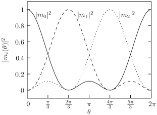
Figure 1: The moduli squared of the three coefficients $m_{j}(\theta)$ in $\sum_{j=0}^{2}m_{j}(\theta)q^{j}$, the Lagrange interpolation between the three unitary matrices $q^{0}$, $q^{1}$, and $q^{2}$.

There exist various different expressions equivalent to (1):

$$m(\theta) = \frac{1}{p}\ \sum_{j}\ \omega^{j}\,q^{j}\,\prod_{k\neq j}(e^{i\theta}-\omega^{k})$$ (4)

$$m(\theta) = \frac{1}{p}\ (e^{ip\theta}-1)\ \sum_{j}\ \frac{\omega^{j}}{e^{i\theta}-\omega^{j}}\ q^{j}$$ (5)

$$m(\theta) = \frac{1}{p}\ \sum_{j}q^{j}\sum_{r}\ \omega^{-rj}e^{ir\theta}\ .$$ (6)

Appendix A describes how they are deduced from (1). Eqn (4) is more compact than eqn (1), as it contains only one instead of two products. Expression (5) corresponds with the so-called ‘first barycentric form’ of the Lagrange interpolation formula. It has the advantage that it contains no product at all. However, it has a disadvantage with respect to (4): in eqn (4) we clearly see that $m$ is a polynomial (of degree $p-1$) in the variable $e^{i\theta}$; in eqn (5) this fact is hidden. The expression (6) constitutes a good compromise between (4) and (5): we still recognize the polynomial nature of the expression, while the sum of products in (4) is simplified to a sum of sums in (6).

In Appendix B, we prove that $m(\theta)$ has the property

$$m(\theta_{1})m(\theta_{2})=m(\theta_{1}+\theta_{2})\ ,$$

such that the multiplication of two $m(\theta)$ matrices yields a third $m(\theta)$ matrix. In particular we have $m(\theta)m(-\theta)=m(0)=u$, such that $m(\theta)^{-1}=m(-\theta)$. Hence, all conditions are fulfilled to say that the set $m(\theta)$, together with the operation of ‘ordinary matrix multiplication’, forms a group. It is a continuous group: a 1-dimensional Lie group. In Appendix C we demonstrate that the matrices $m(\theta)$ are unitary. We thus may conclude that the group is isomorphic to the unitary group U(1).

Any 1-dimensional Lie group $m(\theta)$ has a generator:

$$g=\frac{1}{i}\ \lim_{\theta\rightarrow 0}\frac{dm}{d\theta}\ .$$

With the help of (5) we find:

$$g = \sum_{j\neq 0}\ \frac{\omega^{j}}{1-\omega^{j}}\ q^{j}+\lim\,[\ \frac{e^{ip\theta}}{e^{i\theta}-1}-\frac{(e^{ip\theta}-1)e^{i\theta}}{p\,(e^{i\theta}-1)^{2}}\ ]\ q^{0}$$

$$= \frac{p-1}{2}\ q^{0}+\sum_{j\neq 0}\ \frac{\omega^{j}}{1-\omega^{j}}\ q^{j}\ .$$

With the help of (6) we find an alternative expression for this $n\times n$ matrix:

$$g=\frac{1}{p}\ \sum_{j}\ q^{j}\ \sum_{r}\ r\,\omega^{-rj}\ .$$

For the case $p=2$, both expressions simplify to $g=(q^{0}-q^{1})/2$, a result that can also be retrieved directly from (2).

3 Examples

The $n\times n$ unitary matrices form the unitary group U($n$). Within this infinite group figures the finite subgroup P($n$) of all $n\times n$ permutation matrices. We choose as matrix $q$ of the previous section, one of these $n!$ permutation matrices. Such matrix generates a finite set of matrices $\{q,q^{2},...,q^{p}\}$. This set is a subgroup of P($n$), isomorphic to the cyclic group Z_p of order $p$. The value of $p$ depends on the particular choice of the permutation matrix $q$. The minimum value is 1 (for the trivial choice $q=u$); the maximum value is $L(n)$, where $L$ denotes the Landau function [7].

The group P($n$) is isomorphic to the symmetric group S_n. The cycle graph of a finite group depicts its cyclic subgroups. By convention, only the primitive or maximal cycles (i.e. those cycles that are not subsets of another cycle) are shown.

As a first example, we investigate P(2), i.e. the group of all $2\times 2$ permutation matrices. It contains two elements, forming a single 2-cycle:

$\bullet$ the two matrices $q=\left(\begin{array}[]{cc}0&1\\ 1&0\end{array}\right)$ and $q^{2}=\left(\begin{array}[]{cc}1&0\\ 0&1\end{array}\right)=q^{0}$ ,

the matrix $q$ representing the NOT gate. After (2), the interpolation between $q^{0}$ and $q^{1}$ is

$$m(\theta)=\frac{1}{2}\ \left(\begin{array}[]{cc}1+e^{i\theta}&\ 1-e^{i\theta}\\ 1-e^{i\theta}&\ 1+e^{i\theta}\end{array}\right)\ ,$$

called the NEGATOR gate [8]. It is a quantum gate, generalization of the classical gates $m(0)$ (i.e. the IDENTITY gate) and $m(\pi)$ (i.e. the NOT gate). We note that, for any value of the angle $\theta$, both row sums and both column sums of $m(\theta)$ are equal to 1. The generator of $m(\theta)$ is

$$g=\frac{1}{2}\ \left(\begin{array}[]{rr}1&\ -1\\ -1&1\end{array}\right)\ ,$$

a matrix with all line sums equal to 0.

As a second example, we take P(3), i.e. the group of all $3\times 3$ permutation matrices. It consists of $3!=6$ elements, ordered in four maximal cycles:

• three 2-cycles:

  • the two matrices $q=\left(\begin{array}[]{ccc}1&0&0\\ 0&0&1\\ 0&1&0\end{array}\right)$ and $q^{2}=\left(\begin{array}[]{ccc}1&0&0\\ 0&1&0\\ 0&0&1\end{array}\right)=q^{0}$

  • the two matrices $q=\left(\begin{array}[]{ccc}0&1&0\\ 1&0&0\\ 0&0&1\end{array}\right)$ and $q^{2}=\left(\begin{array}[]{ccc}1&0&0\\ 0&1&0\\ 0&0&1\end{array}\right)=q^{0}$

  • the two matrices $q=\left(\begin{array}[]{ccc}0&0&1\\ 0&1&0\\ 1&0&0\end{array}\right)$ and $q^{2}=\left(\begin{array}[]{ccc}1&0&0\\ 0&1&0\\ 0&0&1\end{array}\right)=q^{0}$

• one 3-cycle, consisting of the three matrices

  $$q=\left(\begin{array}[]{ccc}0&1&0\\ 0&0&1\\ 1&0&0\end{array}\right),\ \ q^{2}=\left(\begin{array}[]{ccc}0&0&1\\ 1&0&0\\ 0&1&0\end{array}\right),\mbox{ and }\ q^{3}=\left(\begin{array}[]{ccc}1&0&0\\ 0&1&0\\ 0&0&1\end{array}\right)=q^{0}\ .$$

There exist no longer cycles, as $L(3)=3$. Figure 2 displays the graph.

Figure 2: Cycle graph of the group P(3) of $3\times 3$ permutation matrices.

We now examine the 3-cycle in detail. After (5) and (6), respectively, its unitary interpolation is

$$m(\theta) = \frac{1}{3}\ (e^{i3\theta}-1)\ \left(\ \frac{1}{e^{i\theta}-1}\ q^{0}+\frac{\omega}{e^{i\theta}-\omega}\ q^{1}+\frac{\omega^{2}}{e^{i\theta}-\omega^{2}}\ q^{2}\ \right)$$

$$= \frac{1}{3}\ [\ (e^{i2\theta}+e^{i\theta}+1)\ q^{0}+(\omega e^{i2\theta}+\omega^{2}e^{i\theta}+1)\ q^{1}+(\omega^{2}e^{i2\theta}+\omega e^{i\theta}+1)\ q^{2}\ ]$$

$$= \frac{1}{3}\ \left(\begin{array}[]{ccccc}x^{2}+x+1&&\omega x^{2}+\omega^{2}x+1&&\omega^{2}x^{2}+\omega x+1\\ \omega^{2}x^{2}+\omega x+1&&x^{2}+x+1&&\omega x^{2}+\omega^{2}x+1\\ \omega x^{2}+\omega^{2}x+1&&\omega^{2}x^{2}+\omega x+1&&x^{2}+x+1\end{array}\right)\ ,$$

where $x$ is a short-hand notation for $e^{i\theta}$ and $\omega$ again is the primitive cubic root of unity. As expected, we have $m(0)=q^{0}$, $m(2\pi/3)=q^{1}$, $m(4\pi/3)=q^{2}$, and $m(2\pi)=q^{0}$ again.

We notice that all six line sums (i.e. three row sums and three column sums) of $m(\theta)$ are equal to 1. Therefore, we say that $m$ belongs to the subgroup XU(3) of U(3), described in detail in Appendix B of [8]. Here, XU($n$) is the subgroup of U($n$) consisting of all $n\times n$ unitary matrices with all $2n$ line sums (i.e. $n$ row sums and $n$ column sums) equal to unity [3] [4] [5]. This is no coincidence. In Appendix D, we prove that, if $q$ is a unitary matrix from XU($n$), then also the interpolation is a member of XU($n$).

For the generators of the four cycles we find:

$$\frac{1}{2}\left(\begin{array}[]{ccc}0&0&0\\ 0&1&-1\\ 0&-1&1\end{array}\right),\,\frac{1}{2}\left(\begin{array}[]{ccc}1&-1&0\\ -1&1&0\\ 0&0&0\end{array}\right),\,\frac{1}{2}\left(\begin{array}[]{ccc}1&0&-1\\ 0&0&0\\ -1&0&1\end{array}\right),\,\mbox{ and }\ \frac{1}{3}\left(\begin{array}[]{ccc}3&\omega-1&\omega^{2}-1\\ \omega^{2}-1&3&\omega-1\\ \omega-1&\omega^{2}-1&3\end{array}\right)\ ,$$

respectively. Each has all line sums equal to 0. Separately, each of these generators generates a 1-dimensional subgroup of XU(3); together they generate the full 4-dimensional group XU(3), subgroup of the 9-dimensional group U(3).

4 Classical and quantum computing

Because classical reversible circuits [1] acting on $w$ bits, are represented by matrices from P($2^{w}$) and quantum circuits [2] acting on $w$ qubits, are represented by matrices from U($2^{w}$), we have special attention for the case $n=2^{w}$.

As an example, we investigate the group P(4), representing all possible reversible circuits with 2 bits at the input and 2 bits at the output. There exist $4!=24$ such circuits. Because P(4) is isomorphic to S₄, we investigate the cycle graph of this symmetric group. It consists of six 2-cycles, four 3-cycles, and three 4-cycles. No longer cycles exist, as $L(4)=4$. We have a closer look at one of the 4-cycles:

$$q=\left(\begin{array}[]{cccc}0&1&0&0\\ 0&0&1&0\\ 0&0&0&1\\ 1&0&0&0\end{array}\right),\ \ q^{2}=\left(\begin{array}[]{cccc}0&0&1&0\\ 0&0&0&1\\ 1&0&0&0\\ 0&1&0&0\end{array}\right),\ \ q^{3}=\left(\begin{array}[]{cccc}0&0&0&1\\ 1&0&0&0\\ 0&1&0&0\\ 0&0&1&0\end{array}\right),\ \ q^{4}=\left(\begin{array}[]{cccc}1&0&0&0\\ 0&1&0&0\\ 0&0&1&0\\ 0&0&0&1\end{array}\right)=q^{0}\ .$$

For the interpolation between $u$, $q$, $q^{2}$, and $q^{3}$, we find

$$m(\theta)=\frac{1}{4}\ \left(\begin{array}[]{llll}1+x+x^{2}+x^{3}&1-ix-x^{2}+ix^{3}&1-x+x^{2}-x^{3}&1+ix-x^{2}-ix^{3}\\ 1+ix-x^{2}-ix^{3}&1+x+x^{2}+x^{3}&1-ix-x^{2}+ix^{3}&1-x+x^{2}-x^{3}\\ 1-x+x^{2}-x^{3}&1+ix-x^{2}-ix^{3}&1+x+x^{2}+x^{3}&1-ix-x^{2}+ix^{3}\\ 1-ix-x^{2}+ix^{3}&1-x+x^{2}-x^{3}&1+ix-x^{2}-ix^{3}&1+x+x^{2}+x^{3}\end{array}\right)\ .$$

We note that the matrix $Q=q^{2}$ not only belongs to this 4-cycle, but also is member of a 2-cycle (although not a maximal 2-cycle):

$$Q=\left(\begin{array}[]{cccc}0&0&1&0\\ 0&0&0&1\\ 1&0&0&0\\ 0&1&0&0\end{array}\right),\ \ Q^{2}=\left(\begin{array}[]{cccc}1&0&0&0\\ 0&1&0&0\\ 0&0&1&0\\ 0&0&0&1\end{array}\right)=Q^{0}\ .$$

For the interpolation between $u$ and $Q$, we find the Lagrange interpolation

$$M(\theta)=\frac{1}{2}\ \left(\begin{array}[]{cccc}1+x&0&\ 1-x&0\\ 0&\ \ 1+x&0&1-x\\ 1-x&0&1+x&0\\ 0&1-x&0&1+x\end{array}\right)\ ,$$

different from $m(\theta)$. Figure 3 displays both the 4-cycle and the 2-cycle.

Figure 3: One maximal 4-cycle and one non-maximal 2-cycle of the group P(4) of $4\times 4$ permutation matrices.

Although we have $M(0)=m(0)=u$ and $M(\pi)=m(\pi)=Q$, we have $M(\pi/2)\neq m(\pi/2)$. Indeed, $m(\pi/2)=q$ is a permutation matrix, whereas $M(\pi/2)$ is a complex unitary matrix:

$$m(\pi/2)=\left(\begin{array}[]{cccc}0&1&0&0\\ 0&0&1&0\\ 0&0&0&1\\ 1&0&0&0\end{array}\right)\ \mbox{ and }\ M(\pi/2)=\frac{1}{2}\ \left(\begin{array}[]{cccc}1+i&0&\ 1-i&0\\ 0&\ \ 1+i&0&1-i\\ 1-i&0&1+i&0\\ 0&1-i&0&1+i\end{array}\right)\ .$$

They represent the circuits

repectively. The former is the cascade of a controlled NOT and a NOT; the latter is a square root of NOT (a.k.a. a V gate). The former is a classical circuit; the latter is a quantum circuit. Both circuits are square roots of the classical circuit

with matrix representation $Q$. We close this section by remarking that the above two matrix sets $m(\theta)$ and $M(\theta)$, both 1-dimensional interpolations between the unit matrix and the matrix $Q$, illustrate that a unitary interpolation between two unitary matrices is not necessarily unique.

Efficient circuit design applying V gates, controlled V gates, W gates, or controlled W gates [10] [11], can be interpreted as using cycles of dyadic $2\times 2$ unitary matrices [12] as matrix $q$ of Section 2, rather than permutation matrices.

5 Conclusion

By Lagrange interpolation, it is possible to embed a finite cyclic group in a 1-dimensional cyclic Lie group. By applying this technique to a cycle of an $n\times n$ permutation matrix, one obtains a 1-dimensional subgroup of the unitary group U($n$). In this way, we can bridge the gap between classical reversible computation (represented by permutation matrices) and quantum computation (represented by unitary matrices).

Appendix 0.A Alternative expressions for the Lagrange interpolation

Assume the numbers $\omega^{0}$, $\omega^{1}$, $\omega^{2}$, …, and $\omega^{p-1}$ are the $p$ solutions of the equation $x^{p}$ $-1$ = 0. Hence:

$$x^{p}-1=\prod_{k}\,(x-\omega^{k})\ ,$$

such that

$$\prod_{k\neq j}(x-\omega^{k})=\frac{x^{p}-1}{x-\omega^{j}}\ .$$ (8)

We apply this result twice:

• With $x=\omega^{j}\,e^{i\epsilon}$ and subsequently $\epsilon\rightarrow 0$ we obtain

  $$\prod_{k\neq j}(\omega^{j}-\omega^{k})=\lim_{\epsilon\rightarrow 0}\ \frac{\omega^{pj}e^{ip\epsilon}-1}{\omega^{j}e^{i\epsilon}-\omega^{j}}=\lim_{\epsilon\rightarrow 0}\ \frac{e^{ip\epsilon}-1}{\omega^{j}(e^{i\epsilon}-1)}=\frac{1}{\omega^{j}}\ \lim_{\epsilon\rightarrow 0}\ \frac{ip\epsilon}{i\epsilon}=\frac{p}{\omega^{j}}\ ,$$

  such that (1) becomes (4).

• With $x=e^{i\theta}$ we obtain

  $$\prod_{k\neq j}(e^{i\theta}-\omega^{k})=\frac{e^{ip\theta}-1}{e^{i\theta}-\omega^{j}}\ ,$$

  such that (4) becomes (5).

Eqn (6) is obtained from eqn (4) by computing $\omega^{j}\,\prod_{k\neq j}(e^{i\theta}-\omega^{k})$. We find its value as follows:

$$\sum_{r}\ \omega^{-rj}x^{r} = \sum_{r}\ (\omega^{-j}x)^{r}$$

$$= \frac{(\omega^{-j}x)^{p}-1}{\omega^{-j}x-1}$$

$$= \frac{\omega^{-jp}x^{p}-1}{\omega^{-j}x-1}$$

$$= \frac{x^{p}-1}{\omega^{-j}x-1}$$

$$= \omega^{j}\,\frac{x^{p}-1}{x-\omega^{j}}$$

$$= \omega^{j}\prod_{k\neq j}(x-\omega^{k})\ .$$

Appendix 0.B Proof of the group structure of the Lagrange interpolation

Assume a general operator (e.g. in matrix form) $\hat{a}$ of the following form

$$\hat{a}=\sum_{j=0}^{p-1}a_{j}\hat{q}^{j}\ ,$$

with $a_{i}\in\mathbb{C}$ elements over the complex field, and $\hat{q}^{p}=1$. From now on, we will omit the operator hat notation on the $q$ operators. First, a straightforward rearrangement shows that

Lemma 1

Given two operators $\hat{a}$ and $\hat{b}$, then the product operator

$$\hat{c}=\hat{a}\hat{b}$$

has coefficients

$$c_{i}=\sum_{m=0}^{i}a_{m}b_{i-m}+\sum_{m=i+1}^{p-1}a_{m}b_{p+i-m}\ .$$

Note that, in $c_{i}$, the indices of the coefficients of $\hat{a}$ and $\hat{b}$ add up to $i$ in the first summation and to $p+i$ in the second summation. We take the summations to be strictly increasing, such that the second term of $c_{p-1}$ vanishes by definition.

Proof. The proof is based on a simple rearrangement of terms. Explicitly, one can write

$$\hat{a}\hat{b}=\sum_{j=0}^{p-1}\sum_{k=0}^{p-1}a_{j}b_{k}q^{j+k}\ ,$$ (9)

and break this double summation down in three different regions, corresponding to respectively regions (A), (B) and (C) in Figure 4,

$$\hat{a}\hat{b}=\sum_{j=0}^{p-2}\sum_{k=0}^{p-j-2}a_{j}b_{k}q^{j+k}+\sum_{j=0}^{p-1}a_{j}b_{p-j-1}q^{p-1}+\sum_{j=1}^{p-1}\sum_{k=p-j}^{p-1}a_{j}b_{k}q^{j+k}\ .$$

Figure 4: Decomposition of the summation in eq. (9).

A change of dummy summation indices $\{i=j+k,l=\frac{1}{2}(k-j)\}$ gives

$$\hat{a}\hat{b} = \sum_{i=0}^{p-2}\sum_{l=-\frac{i}{2}}^{\frac{i}{2}}a_{\frac{i}{2}-l}b_{\frac{i}{2}+l}\ q^{i}+\sum_{l=-\frac{p}{2}+\frac{1}{2}}^{\frac{p}{2}-\frac{1}{2}}a_{\frac{p}{2}-\frac{1}{2}-l}b_{\frac{p}{2}-\frac{1}{2}+l}\ q^{p-1}$$

$$+\sum_{i=p}^{2p-2}\sum_{l=\frac{i}{2}-p+1}^{p-1-\frac{i}{2}}a_{\frac{i}{2}-l}b_{\frac{i}{2}+l}\ q^{i}\ .$$

The index $i$ is always larger (or equal) to $p$ in the last summation, such that

$$\hat{a}\hat{b} = \sum_{i=0}^{p-2}\sum_{l=-\frac{i}{2}}^{\frac{i}{2}}a_{\frac{i}{2}-l}b_{\frac{i}{2}+l}\ q^{i}+\sum_{l=-\frac{p}{2}+\frac{1}{2}}^{\frac{p}{2}-\frac{1}{2}}a_{\frac{p}{2}-\frac{1}{2}-l}b_{\frac{p}{2}-\frac{1}{2}+l}\ q^{p-1}$$

$$+\sum_{m=0}^{p-2}\sum_{l=\frac{m}{2}-\frac{p}{2}+1}^{\frac{p}{2}-1-\frac{m}{2}}a_{\frac{p}{2}+\frac{m}{2}-l}b_{\frac{p}{2}+\frac{m}{2}+l}\ q^{m}\ ,$$

where $q^{p}=1$ has been used. Reintroducing dummy summation index $j=\frac{i}{2}-l$ in the first summation, while defining it as $j=\frac{p}{2}-\frac{1}{2}-l$ in the second, and $j=\frac{p}{2}+\frac{m}{2}-l$ in the last, we obtain

$$\hat{a}\hat{b}=\sum_{i=0}^{p-2}\sum_{j=0}^{i}\,a_{j}b_{i-j}q^{i}+\sum_{j=0}^{p-1}\,a_{j}b_{p-1-j}q^{p-1}+\sum_{i=0}^{p-2}\sum_{j=i+1}^{p-1}\,a_{j}b_{p+i-j}q^{i}\ .$$

This leads us to

$$\hat{a}\hat{b}=\sum_{i=0}^{p-1}\left[\sum_{m=0}^{i}a_{m}b_{i-m}+\sum_{m=i+1}^{p-1}a_{m}b_{p+i-m}\right]q^{i}\ ,$$

which completes the proof of the lemma.

The 1-parameter group structure of the Lagrange interpolation operators can now be proven. As demonstrated in Appendix A, there are multiple representations for the $m_{j}$ coefficients in (3). We will employ here expression (5):

$$m_{j}(\theta)=\frac{1}{p}\ \frac{e^{ip\theta}-1}{e^{i\theta}-\omega^{j}}\ \omega^{j}\ .$$

Lemma 2

Given two Lagrange interpolation operators $\hat{m}(\theta_{1})$ and $\hat{m}(\theta_{2})$ with coefficients

$$m_{j}(\theta_{k})=\frac{1}{p}\ \frac{e^{ip\theta_{k}}-1}{e^{i\theta_{k}}-\omega^{j}}\ \omega^{j}\ \mbox{ for }\ k\in\{1,2\}\ ,$$

then the product operator $\hat{a}=\hat{m}(\theta_{1})\hat{m}(\theta_{2})$ has coefficients

$$a_{j}=\frac{1}{p}\ \frac{e^{ip(\theta_{1}+\theta_{2})}-1}{e^{i(\theta_{1}+\theta_{2})}-\omega^{j}}\ \omega^{j}\ .$$

Proof. The previous lemma states that

$$a_{j} = \sum_{m=0}^{j}\frac{1}{p}\ \frac{e^{ip\theta_{1}}-1}{e^{i\theta_{1}}-\omega^{m}}\ \omega^{m}\ \frac{1}{p}\ \frac{e^{ip\theta_{2}}-1}{e^{i\theta_{2}}-\omega^{j-m}}\ \omega^{j-m}$$

$$+\sum_{m=j+1}^{p-1}\frac{1}{p}\ \frac{e^{ip\theta_{1}}-1}{e^{i\theta_{1}}-\omega^{m}}\ \omega^{m}\ \frac{1}{p}\ \frac{e^{ip\theta_{2}}-1}{e^{i\theta_{2}}-\omega^{p+j-m}}\ \omega^{p+j-m}\ .$$

Using $\omega^{p}=1$, this can be shortened to

$$a_{j}=\frac{1}{p^{2}}\ (e^{ip\theta_{1}}-1)(e^{ip\theta_{2}}-1)\,\omega^{j}\left[\sum_{m=0}^{p-1}\frac{1}{e^{i\theta_{1}}-\omega^{m}}\ \frac{1}{e^{i\theta_{2}}-\omega^{j-m}}\right]\ .$$ (10)

The summation in (10) can be reduced using partial fractions:

$$\sum_{m=0}^{p-1} \!\!\!\frac{1}{e^{i\theta_{1}}-\omega^{m}}\ \frac{1}{e^{i\theta_{2}}-\omega^{j-m}}$$ (11)

$$= \frac{1}{e^{i\theta_{2}}}\ \sum_{m=0}^{p-1}\frac{1}{e^{i\theta_{1}}-\omega^{m}}\ \frac{\omega^{m}}{\omega^{m}-\omega^{j}e^{-i\theta_{2}}}$$

$$= \frac{1}{e^{i(\theta_{1}+\theta_{2})}-\omega^{j}}\sum_{m=0}^{p-1}\left[\frac{\omega^{m}}{e^{i\theta_{1}}-\omega^{m}}+\frac{\omega^{m}}{\omega^{m}-\omega^{j}e^{-i\theta_{2}}}\right]$$

$$= \frac{1}{e^{i(\theta_{1}+\theta_{2})}-\omega^{j}}\sum_{m=0}^{p-1}\left[\frac{e^{i\theta_{1}}-e^{i\theta_{1}}+\omega^{m}}{e^{i\theta_{1}}-\omega^{m}}+\frac{\omega^{m}-\omega^{j}e^{-i\theta_{2}}+\omega^{j}e^{-i\theta_{2}}}{\omega^{m}-\omega^{j}e^{-i\theta_{2}}}\right]$$

$$= \frac{1}{e^{i(\theta_{1}+\theta_{2})}-\omega^{j}}\left(e^{i\theta_{1}}\sum_{m=0}^{p-1}\frac{1}{e^{i\theta_{1}}-\omega^{m}}-\omega^{j}e^{-i\theta_{2}}\sum_{m=0}^{p-1}\frac{1}{\omega^{j}e^{-i\theta_{2}}-\omega^{m}}\right)\,.$$

This formula can be even further reduced by realizing that

$$\sum_{m=0}^{p-1}\prod_{k\neq m}(x-\omega^{k})=\frac{d}{dx}\ \prod_{k}(x-\omega^{k})=\frac{d}{dx}(x^{p}-1)=px^{p-1}$$ (12)

and thus

$$\sum_{m=0}^{p-1}\frac{1}{x-\omega^{m}}\ =\sum_{m=0}^{p-1}\ \frac{\prod_{k\neq m}(x-\omega^{k})}{\prod_{k}(x-\omega^{k})}=\frac{1}{\prod_{k}(x-\omega^{k})}\sum_{m=0}^{p-1}\ \prod_{k\neq m}(x-\omega^{k})=\frac{px^{p-1}}{x^{p}-1}\ .$$

Inserting this relation in both sums of (11), we gather

$$\sum_{m=0}^{p-1} \!\!\!\frac{1}{e^{i\theta_{1}}-\omega^{m}}\ \frac{1}{e^{i\theta_{2}}-\omega^{j-m}}$$

$$= \frac{1}{e^{i(\theta_{1}+\theta_{2})}-\omega^{j}}\ \left(e^{i\theta_{1}}\ \frac{pe^{i(p-1)\theta_{1}}}{e^{ip\theta_{1}}-1}-\omega^{j}e^{-i\theta_{2}}\ \frac{p\omega^{(p-1)j}e^{-i(p-1)\theta_{2}}}{\omega^{pj}e^{-ip\theta_{2}}-1}\right)$$

$$= \frac{p}{e^{i(\theta_{1}+\theta_{2})}-\omega^{j}}\ \frac{1-e^{ip(\theta_{1}+\theta_{2})}}{(e^{ip\theta_{1}}-1)(1-e^{ip\theta_{2}})}\ ,$$

in which we have used that $\omega^{p}=1$. Inserting this result in eq. (10) leads to

$$a_{j}=\frac{1}{p}\ \frac{e^{ip(\theta_{1}+\theta_{2})}-1}{e^{i(\theta_{1}+\theta_{2})}-\omega^{j}}\ \omega^{j}=m_{j}(\theta_{1}+\theta_{2})\ .$$

This means that $\hat{m}(\theta_{1})\hat{m}(\theta_{2})$ equals $\hat{m}(\theta_{1}+\theta_{2})$, which is what had to be proven.

Appendix 0.C Proof of the unitarity of the Lagrange interpolation

Because of Appendix B we have the matrix equality $m(\theta_{1})m(\theta_{2})=m(\theta_{1}+\theta_{2})$, and hence, in particular, $m(\theta)m(-\theta)=u$ or $m(\theta)^{-1}=m(-\theta)$. We compute $m(-\theta)$ from (1) by changing from indices $j$ and $k$ to indices $J=p-j$ and $K=p-k$:

$$m(-\theta) = \sum_{j}\ \frac{\prod_{k\neq j}(e^{-i\theta}-\omega^{k})}{\prod_{k\neq j}(\omega^{j}-\omega^{k})}\ q^{j}$$

$$= \sum_{J}\ \frac{\prod_{K\neq J}(e^{-i\theta}-\omega^{p-K})}{\prod_{K\neq J}(\omega^{p-J}-\omega^{p-K})}\ q^{p-J}$$

$$= \sum_{J}\ \frac{\prod_{K\neq J}(e^{-i\theta}-\omega^{-K})}{\prod_{K\neq J}(\omega^{-J}-\omega^{-K})}\ q^{-J}$$

$$= \sum_{J}\ \frac{\prod_{K\neq J}(e^{-i\theta}-\overline{\omega}^{K})}{\prod_{K\neq J}(\overline{\omega}^{J}-\overline{\omega}^{K})}\ (q^{\dagger})^{J}$$

$$= [\,m(\theta)\,]^{\dagger}\ ,$$

where we took into account that $q$ is unitary: $q^{-1}=q^{\dagger}$.

We can conclude that $m(\theta)^{-1}$ equals $[\,m(\theta)\,]^{\dagger}$ and thus that $m(\theta)$ is unitary.

Appendix 0.D Proof of the XU property of the Lagrange interpolation

For the classical Lagrange interpolation, the sum of the Lagrange fundamental polynomials is equal to unity, a property known as the first Cauchy relation [6] [9]. We prove here that a similar property holds for the matrix interpolation (1)-(3):

$$\sum_{j}m_{j}(\theta)=1\ .$$

Indeed, by applying eqn (4), we find:

$$\sum_{j}m_{j}(\theta) = \frac{1}{p}\ \sum_{j}\ \omega^{j}\ \prod_{k\neq j}(x-\omega^{k})$$

$$= -\ \frac{1}{p}\ \sum_{j}\ [\ (x-\omega^{j})-x\ ]\ \prod_{k\neq j}(x-\omega^{k})$$

$$= -\ \frac{1}{p}\ \sum_{j}\ (x-\omega^{j})\ \prod_{k\neq j}(x-\omega^{k})+\frac{x}{p}\ \sum_{j}\ \prod_{k\neq j}(x-\omega^{k})\ .$$

Applying (8) for the former sum and (12) for the latter sum, we obtain

$$-\ (x^{p}-1)+x^{p}$$

and thus unity.

If a matrix $q$ belongs to the group XU($n$), then all $q^{j}$ belong to XU($n$). Because the row sum of a sum of matrices equals the sum of the row sums of the constituent matrices, the row sum of $m=\sum_{j}m_{j}q^{j}$ equals $\sum_{j}m_{j}$ times the unit row sum of $q^{j}$ and thus equals $\sum_{j}m_{j}$. Because of the above Cauchy relation, this quantity is equal to 1. Hence, the matrix $m$ has all $n$ row sums equal to unity. We obtain a similar result for the $n$ column sums. Hence, the interpolation matrix $m$ belongs to XU($n$). In fact, the matrices $m(\theta)$ constitute a 1-dimensional subgroup of the $(n-1)^{2}$-dimensional group XU($n$).

References

[1] De Vos, A.:
Reversible computing.
Wiley–VCH, Weinheim (2010)
[2] Nielsen, M., Chuang, I.:
Quantum computation and quantum information.
Cambridge University Press, Cambridge (2000)
[3] De Vos, A., De Baerdemacker, S.:
The decomposition of U() into XU() and ZU().
Proceedings of the 44 th International Symposium on
Multiple-Valued Logic,
Bremen, 19-21 May 2014, pp. 173–177
[4] De Vos, A., De Baerdemacker, S.:
On two subgroups of U(), useful for quantum computing.
Journal of Physics: Conference Series:
Proceedings of the 30 th International Colloquium on
Group-theoretical Methods in Physics,
Gent, 14-18 July 2014
[5] De Vos, A., De Baerdemacker, S.:
Matrix calculus for classical and quantum circuits.
ACM Journal on Emerging Technologies in Computing Systems,
volume 11, 9 (2014)
[6] Davis, P.:
Interpolation and approximation.
Dover Publications, New York (1975)
[7] Landau, E.:
Über die Maximalordnung der Permutationen gegebenen Grades.
Archiv der Mathematik und Physik, 3. Reihe,
volume 5, 92–103 (1903)
[8] De Vos, A., De Baerdemacker, S.:
The NEGATOR as a basic building block for quantum circuits.
Open Systems & Information Dynamics,
volume 20, 1350004 (2013)
[9] Fichtner, A.:
SES3D version 2.1.
www.geophysik.uni-muenchen.de/~fichtner/ses3d. pdf (2009)
[10] Rahman, M., Dueck, G., Banerjee, A.:
Optimization of reversible circuits using reconfigurable templates.
Proceedings of the 3 rd International Workshop on
Reversible Computation,
Gent, 4-5 July 2011,
Springer Lecture Notes in Computer Science 7165, Berlin (2012), pp. 43-53
[11] Sasanian, Z., Miller, D.:
Transforming MCT circuits to NCVW circuits.
Proceedings of the 3 rd International Workshop on
Reversible Computation,
Gent, 4-5 July 2011,
Springer Lecture Notes in Computer Science 7165, Berlin (2012), pp. 77-88
[12] De Vos, A., Van Laer, R., Vandenbrande, S.:
The group of dyadic unitary matrices.
Open Systems & Information Dynamics,
volume 19, 1250003 (2012)